About convergence proof of robust multigrid technique

ISSN 2070�0482, Mathematical Models and Computer Simulations, 2011, Vol. 3, No. 3, pp. 333–345. © Pleiades Publishing, Ltd., 2011.Original Russian Text © S.I. Martynenko, 2010, published in Matematicheskoe Modelirovanie, 2010, Vol. 22, No. 10, pp. 18–34.

333

1. INTRODUCTION

The numerical solution of a boundary value problem can be reduced to the solution of a system of lin�ear algebraic equations (SLAE) with sparse coefficient matrix of high order. In order to solve the givenSLAE

Ax = b (1)we use the iteration method of type

W(x(n + 1) – x(n)) = b – Ax(n), (2)where W is some matrix. The next approximation to the solution is computed as follows:

(3)

Matrix S = I – W–1A is called the iteration matrix. In the case where ||S|| ≤ q < 1, iterative method (3) con�verges as fast as a geometric progression with the index q for an arbitrary initial approximation x(0) and rightpart b [1].

Let us vewrite the system (1). Let x(n) be an approximation to the solution of system (1), satisfying theequation

where r is some residual, be known. Add some correction c to x(n) in order to delete the residual r, i.e.,

To solve system

(4)one can use iterative method (2), written as

or

(5)

it is natural to choose the zero starting guess c(0) = 0. After ν iterations have been executed, the nextapproximation x(n + 1) to the solution of system (1) is computed as follows:

x n 1+( ) I W 1– A–( )x n( ) W 1– b.+=

Ax n( ) b r,+=

A x n( ) c+( ) b.=

Ac b Ax n( )–=

c ν( ) Sc ν 1–( ) W 1– b Ax n( )–( )+=

c ν( ) Sνc 0( ) SkW 1– b Ax n( )–( ),k 0=

ν 1–

∑+=

x n 1+( ) x n( ) c ν( )+ I SkW 1– Ak 0=

ν 1–

∑–⎝ ⎠⎜ ⎟⎛ ⎞

x n( ) SkW 1– b.

k 0=

ν 1–

∑+= =

About Convergence Proof of Robust Multigrid TechniqueS. I. Martynenko

Baranov Central Institute of Aviation Motors Development, ul. Aviamotornaya 2, Moscow, 111116 Russiae�mail: [email protected]

Received September 28, 2009

Abstract—The article presents the analysis of the convergence of a robust multigrid technique. Anestimation of the norm of a multigrid iteration matrix with account of the approximation property isobtained.

Keywords: multigrid methods, the convergence of multigrid iterations

DOI: 10.1134/S2070048211030082

334

MATHEMATICAL MODELS AND COMPUTER SIMULATIONS Vol. 3 No. 3 2011

MARTYNENKO

As a rule, the convergence rateof the iterative methods (3) or (5) issmall when sufficiently fine gridsare used. Therefore, the develop�ment of efficient iterative methodsfor the solution of the SLAE result�ing from the approximation ofboundary value problems has beenthe subject of much investigation.At present, one of the most popularmethods for the solution of suchSLAE is classical multigrid meth�ods (CMM) having optimal con�vergence rate (i.e. independent onthe grid mesh size) [1]. The highconvergence rate of CMM isobtained by adaptation of theircomponents to the solved problem.As a result, it is difficult to useCMM in black box software.

Therefore original variant of multigrid methods with problem�independent transfer operators referred asa robust multigrid technique (RMT) has been proposed and developed [2–4].

Convergence proof of the multigrid methods is a challenging problem. On the one hand, single differ�ence the multigrid methods and iterative solver (5) is that the starting guess c0 is not given (as zero) andcomputed on coarse grids. On the other hand, it is difficult to estimate the iteration matrix norm and oftenit can done in the simplest cases with some assumptions.

2. AN ILLUSTRATIVE EXAMPLE

RMT differs from CMM in construction of the difference equations on coarse grids and transfer oper�ators. We demonstrate the differences with the following one�dimensional (1D) boundary value problemfor Poisson equation

(6)

which the exact solution

(7)

(8)

Substitution of (8) into (6) results in the Σ�modified form of the original problem, where is a correc�tion and is an approximation to the solution. The substitution of (8) into (6) results in the Σ�modifiedform of notation of the original problem:

(9)

The solution is represented in form (8) before the discretization of the initial boundary value problem.This representation offers new possibilities in application of RMT as a preconditioner.

Next, we construct a uniform grid by breaking interval [0, 1] into H = 10 parts

where and are the vertices and the control volume faces, and h = H–1 is a mesh size.

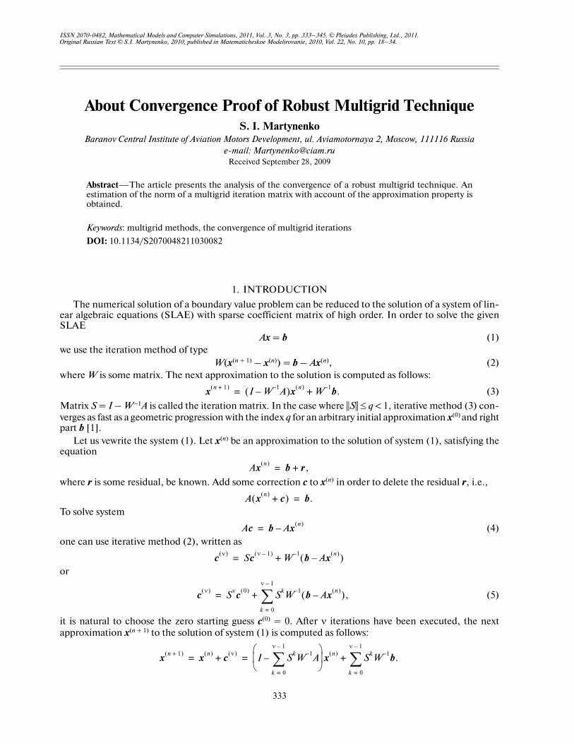
In N�dimensional case the finest grid generates 3N coarse grids forming the first level. Similarly, all gridsof the first level generate 32N coarser grids forming the second level. The coarse grid generation is finished

d2u

dx2�� 10ex

, u 0( ) u 1( ) 0,= = =

u x( ) 10 ex 1 e–( )x 1–+( ),=

u x( ) c x( ) u x( ).+=

c x( )u x( )

d2 c

dx2�� 10ex d2u

dx2��, c 0( )– c 1( ) 0, u 0( ) u 1( ) 0.= = = = =

G10

xiv i 1–( )h, i 1 … H 1,+, ,= =

xif i 1

2��–⎝ ⎠

⎛ ⎞ h, i 1 … H,, ,= =

xiv xi

f

xf1

G01

G11

xv1

xf2 xf

3 xf4 xf

5 xf6 xf

7 xf8 xf

9xv

2 xv3 xv

4 xv5 xv

6 xv7 xv

8 xv9 xv

10

G01

G01

G12

G13

The finest grid

The first grid on the first level

The second grid on the first level

The third grid on the first level

The finest grid

The finest grid

Fig. 1. Coarsening in RMT.


ABOUT CONVERGENCE PROOF OF ROBUST MULTIGRID TECHNIQUE 335

when the coarsest grids have only several gridpoints.

In RMT smoothing on the multigrid struc�ture makes it possible to avoid the occurrence ofextra problem�dependent components as com�pared with single�grid algorithms. The multi�grid structure consists of l levels (l = 0, 1, …,L+), and for each l, the level comprises 3Nl grids(N = 2 or 3). The level with l = 0 comprises the

single finest grid and the level with l = L+

comprises the coarsest grids. The numberof the level with the coarsest grids is specifiedbefore the multigrid structure is built. Let thefinest grid consist of Hx × Hy × Hz points. Then,

G10,

3NL+

where

the square brackets signify the integer part [2–4].

In the RMT, the coarse grids are constructed by tripling the pitch, not by doubling, as in the CMM,and feature the following properties:

Property 1. Each control volume in grids (l = 0, 1, …, L+ and k = ) can be represented as a

union of 3Nl control volumes in the finest grid

Property 2. Each grid (l ≠ L+) can be represented as a union of 3N appropriate coarse grids. Conse�

quently, the finest grid can be represented as a union of all grids on the same level:

Property 3. Grids that are on the same level have no points in common:

We approximate Σ�modified boundary value problem (9) for coarse grids and by the con�trol volume discretization.

The integration of Eq. (9) over control volume yields the following difference relation�ship:

(10)

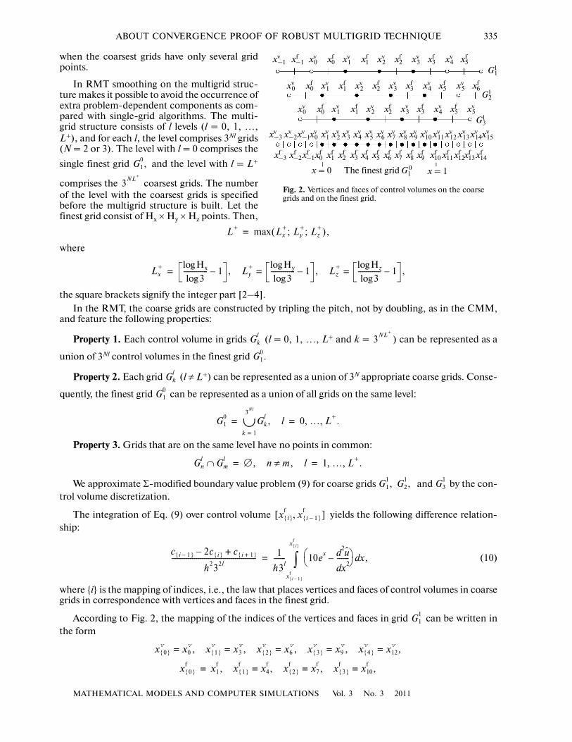
where {i} is the mapping of indices, i.e., the law that places vertices and faces of control volumes in coarsegrids in correspondence with vertices and faces in the finest grid.

According to Fig. 2, the mapping of the indices of the vertices and faces in grid can be written inthe form

L+max Lx

+; Ly

+; Lz

+( ),=

Lx+ Hxlog

3log�� 1– , Ly

+ Hylog

3log�� 1– , Lz

+ Hzlog

3log�� 1– ,===

Gkl 3NL

+

G10.

Gkl

G10

G10 Gk

l, l

k 1=

3Nl

∪ 0 … L+., ,= =

Gnl Gm

l∩ ∅, n m, l≠ 1 … L+., ,= =

G11, G2

1, G3

1

x i{ }

f x i 1–{ }

f,[ ]

c i 1–{ } 2c i{ } c i 1+{ }+–

h232l�� 1

h3l�� 10ex u

2d

x2d��–⎝ ⎠

⎛ ⎞ xd ,

x i 1–{ }

f

x i{ }

f

∫=

G11

x 0{ }

v x0v= , x 1{ }

v x3v

, x 2{ }

v x6v

, x 3{ }

v x9v

, x 4{ }

v x12v

,====

x 0{ }

f x1f, x 1{ }

f x4f, x 2{ }

f x7f, x 3{ }

f x10f

,====

xf1

G11

xv1

xf2 xf

3

xf0

xf5

xf6

xf–1

xv2 xv

3 xv4 xv

5 xv6 xv

7 xv8 xv

9 xv10

The finest grid G 0

xf1 xf

2 xf3 xf

5

xf5xf

3xf2xf

1

xv1

xv1

xv1 xv

2

xv2

xv2 xv

3

xv3

xv3 xv

4

xv4

xv4

xv5

xv5

xv–3 xv

–2xv–1x

v0

xf1 xf

2 xf3 xf

4 xf5 xf

6 xf7 xf

8 xf9xf

–3 xf–2xf

–1xf0

xf0

xv–1 xv

0 xf0

xv0

xv0

G12

G13

x = 0 x = 1

xv11 xv

12 xv13 xv

14xv15

xf10 xf

11 xf12x

f13 xf

14

Fig. 2. Vertices and faces of control volumes on the coarsegrids and on the finest grid.

1

336


MARTYNENKO

that is to say, the first vertex in grid is associated with the third vertex in the finest grid the second

one, with the sixth one, etc. Vertices and are dummy ones, since they lie outside the unit interval.

The right�hand side of (10) is approximated for the finest grid (l = 0) as follows:

We form the vector of the right�hand members (residuals) r with components

(11)

In the first vertex of grid on the first level (l = 1), Eq. (10) assumes the form

The approximation of boundary conditions for coarse grids is fully considered in [2, 3]. In the present

case, the value c{0} in the dummy vertex is eliminated by means of relationship

Because control volume is a union of three control volumes in the finest grid (Property 1),

the right side can then be rewritten as

which, in view of (11), results in

Thus, Eq. (10) in the first vertex of grid on the first level (l = 1) assumes the final form

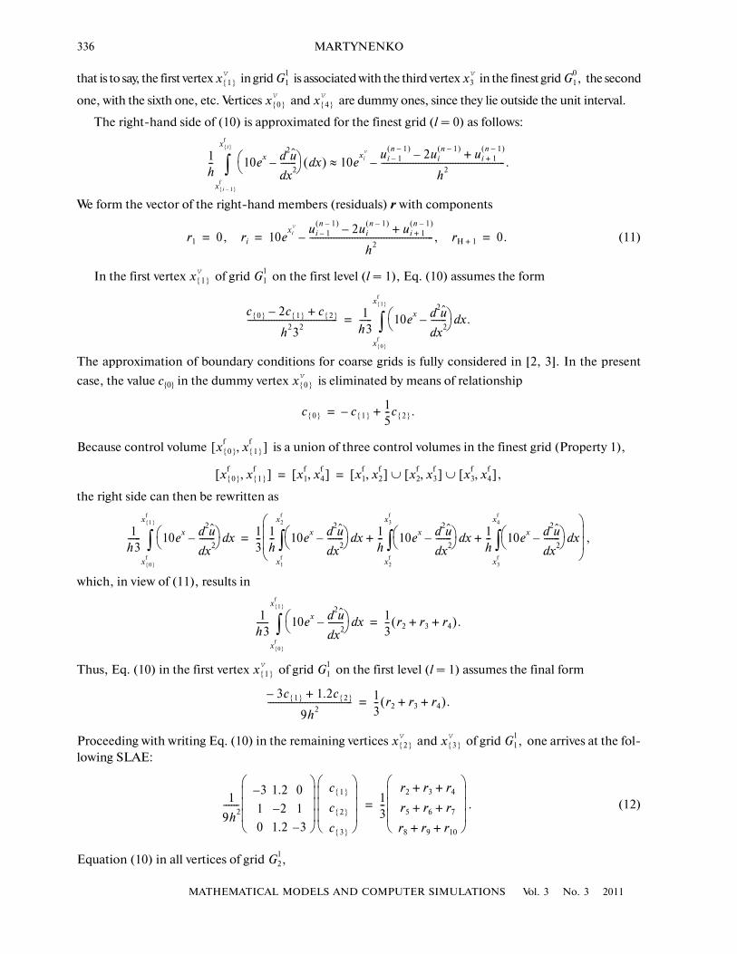
Proceeding with writing Eq. (10) in the remaining vertices and of grid one arrives at the fol�lowing SLAE:

(12)

Equation (10) in all vertices of grid

x 1{ }

v G11 x3

v G10,

x 0{ }

v x 4{ }

v

1h�� 10ex u

2d

x2d��–⎝ ⎠

⎛ ⎞ xd( )

x i 1–{ }

f

x i{ }

f

∫ 10exiv ui 1–

n 1–( ) 2uin 1–( ) ui 1+

n 1–( )+–

h2��.–≈

r1 0, ri 10exiv ui 1–

n 1–( ) 2uin 1–( ) ui 1+

n 1–( )+–

h2��, rH 1+– 0.= = =

x 1{ }

v G11

c 0{ } 2c 1{ }– c 2{ }+

h232�� 1

h3�� 10ex u

2d

x2d��–⎝ ⎠

⎛ ⎞ xd .

x 0{ }

f

x 1{ }

f

∫=

x 0{ }

v

c 0{ } c 1{ }– 15��c 2{ }.+=

x 0{ }

f x 1{ }

f,[ ]

x 0{ }

f x 1{ }

f,[ ] x1f x4

f,[ ] x1f x2

f,[ ] x2f x3

f,[ ] x3f x4

f,[ ],∪ ∪= =

1h3�� 10ex u

2d

x2d��–⎝ ⎠

⎛ ⎞ xd

x 0{ }

f

x 1{ }

f

∫13�� 1

h�� 10ex u

2d

x2d��–⎝ ⎠

⎛ ⎞ xd

x1f

x2f

∫1h�� 10ex u

2d

x2d��–⎝ ⎠

⎛ ⎞ xd

x2f

x3f

∫1h�� 10ex u

2d

x2d��–⎝ ⎠

⎛ ⎞ xd

x3f

x4f

∫+ +⎝ ⎠⎜ ⎟⎜ ⎟⎛ ⎞

,=

1h3�� 10ex u

2d

x2d��–⎝ ⎠

⎛ ⎞ xd

x 0{ }

f

x 1{ }

f

∫13�� r2 r3 r4+ +( ).=

x 1{ }

v G11

3c 1{ }– 1.2c 2{ }+

9h2�� 1

3�� r2 r3 r4+ +( ).=

x 2{ }

v x 3{ }

v G11,

1

9h2��

3– 1.2 0

1 2– 1

0 1.2 3–⎝ ⎠⎜ ⎟⎜ ⎟⎜ ⎟⎛ ⎞ c 1{ }

c 2{ }

c 3{ }⎝ ⎠⎜ ⎟⎜ ⎟⎜ ⎟⎛ ⎞

13��

r2 r3 r4+ +

r5 r6 r7+ +

r8 r9 r10+ +⎝ ⎠⎜ ⎟⎜ ⎟⎜ ⎟⎛ ⎞

.=

G21,



(13)

and

(14)

can be written in much the same way.

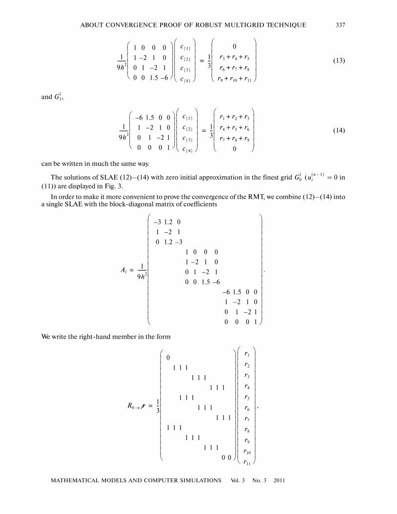
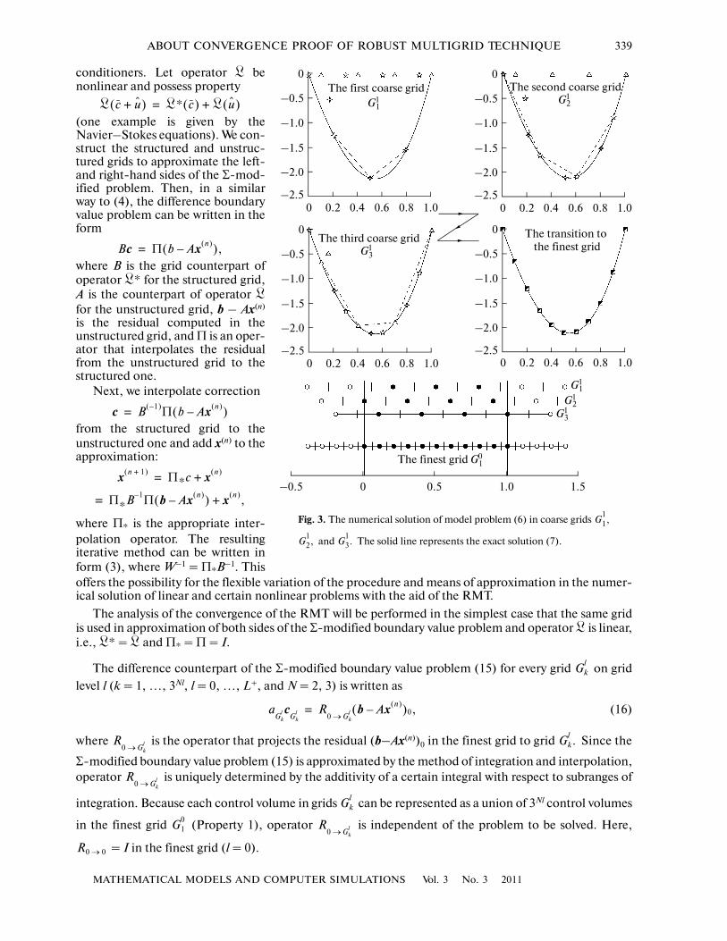
The solutions of SLAE (12)–(14) with zero initial approximation in the finest grid ( = 0 in(11)) are displayed in Fig. 3.

In order to make it more convenient to prove the convergence of the RMT, we combine (12)–(14) intoa single SLAE with the block�diagonal matrix of coefficients

We write the right�hand member in the form

1

9h2��

1 0 0 0

1 2– 1 0

0 1 2– 1

0 0 1.5 6–⎝ ⎠⎜ ⎟⎜ ⎟⎜ ⎟⎜ ⎟⎛ ⎞ c 1{ }

c 2{ }

c 3{ }

c 4{ }⎝ ⎠⎜ ⎟⎜ ⎟⎜ ⎟⎜ ⎟⎜ ⎟⎛ ⎞

13��

0

r3 r4 r5+ +

r6 r7 r8+ +

r9 r10 r11+ +⎝ ⎠⎜ ⎟⎜ ⎟⎜ ⎟⎜ ⎟⎜ ⎟⎛ ⎞

=

G31,

1

9h2��

6– 1.5 0 0

1 2– 1 0

0 1 2– 1

0 0 0 1⎝ ⎠⎜ ⎟⎜ ⎟⎜ ⎟⎜ ⎟⎛ ⎞ c 1{ }

c 2{ }

c 3{ }

c 4{ }⎝ ⎠⎜ ⎟⎜ ⎟⎜ ⎟⎜ ⎟⎜ ⎟⎛ ⎞

13��

r1 r2 r3+ +

r4 r5 r6+ +

r7 r8 r9+ +

0⎝ ⎠⎜ ⎟⎜ ⎟⎜ ⎟⎜ ⎟⎜ ⎟⎛ ⎞

=

G01 ui

n 1–( )

Al1

9h2��

3– 1.2 0

1 2– 1

0 1.2 3–

1 0 0 0

1 2– 1 0

0 1 2– 1

0 0 1.5 6–

6– 1.5 0 0

1 2– 1 0

0 1 2– 1

0 0 0 1⎝ ⎠⎜ ⎟⎜ ⎟⎜ ⎟⎜ ⎟⎜ ⎟⎜ ⎟⎜ ⎟⎜ ⎟⎜ ⎟⎜ ⎟⎜ ⎟⎜ ⎟⎜ ⎟⎜ ⎟⎜ ⎟⎜ ⎟⎛ ⎞

.=

R0 l→ r 13��

0

1 1 1

1 1 1

1 1 1

1 1 1

1 1 1

1 1 1

1 1 1

1 1 1

1 1 1

0 0⎝ ⎠⎜ ⎟⎜ ⎟⎜ ⎟⎜ ⎟⎜ ⎟⎜ ⎟⎜ ⎟⎜ ⎟⎜ ⎟⎜ ⎟⎜ ⎟⎜ ⎟⎜ ⎟⎜ ⎟⎜ ⎟⎜ ⎟⎛ ⎞ r1

r2

r3

r4

r5

r6

r7

r8

r9

r10

r11⎝ ⎠⎜ ⎟⎜ ⎟⎜ ⎟⎜ ⎟⎜ ⎟⎜ ⎟⎜ ⎟⎜ ⎟⎜ ⎟⎜ ⎟⎜ ⎟⎜ ⎟⎜ ⎟⎜ ⎟⎜ ⎟⎜ ⎟⎜ ⎟⎛ ⎞

,=

338


MARTYNENKO

where r is residual (11) computed in the finest grid and R0 → l is the restriction operator that projectsthe residual in the finest grid (zero level, l = 0) onto grids on level l (in the instance under consideration,onto grids on the first level, l = 1). It is obvious that R0 → l is independent of the problem to be solved.

Thus, the combined SLAE assumes the form

and its solution

can be projected onto the level with finer grids,

where Pl → l – 1 is the prolongation operator. In the instance under consideration,

An example of the transition from the first level to the zero level is shown in Fig. 3. It is evident that Pl → l – 1 is atransposition matrix, determined by the finest grid and the numbering of vertices and grids, but indepen�dent of the problem to be solved.

It should be emphasized that the representation of difference equations as a single SLAE is onlyintended to demonstrate the form of transition operators in the RMT and make it more convenient toprove the convergence of the latter. When dealing with applied problems, SLAE of type (12)–(14) aresolved either serially (for single�processor execution) or in parallel (for parallel execution).

3. AN ESTIMATE OF THE NORM OF A MULTIGRID ITERATION MATRIX

Let the initial differential problem

where x ∈ Ω, Ω is a region in the N�dimensional space, f(x) is a specified function, and � is a linear dif�ferentiation operator, be given. It is presumed that the boundary conditions are taken into account inoperator � and the right�hand member f(x). The presentation of the sought solution in the form

makes it possible to rearrange the original problem to the following Σ�modified form

(15)

where the grid counterparts of functions and will act as the correction and approximation to the solu�tion, respectively, in the subsequent multigrid iterations of the RMT.

In the RMT, unlike the CMM, the solution is represented as u = + before, not after, the approxi�mation of the original problem is performed, which opens up new possibilities for the construction of pre�

G10

Alcl R0 l→ r,=

cl Al1– R0 l→ r=

cl 1– Pl l 1–→ cl,=

c1

c2

c3

c4

c5

c6

c7

c8

c9

c10

c11⎝ ⎠⎜ ⎟⎜ ⎟⎜ ⎟⎜ ⎟⎜ ⎟⎜ ⎟⎜ ⎟⎜ ⎟⎜ ⎟⎜ ⎟⎜ ⎟⎜ ⎟⎜ ⎟⎜ ⎟⎜ ⎟⎜ ⎟⎜ ⎟⎛ ⎞

0 0 0 1 0 0 0 0 0 0 0

0 0 0 0 0 0 0 1 0 0 0

1 0 0 0 0 0 0 0 0 0 0

0 0 0 0 1 0 0 0 0 0 0

0 0 0 0 0 0 0 0 1 0 0

0 1 0 0 0 0 0 0 0 0 0

0 0 0 0 0 1 0 0 0 0 0

0 0 0 0 0 0 0 0 0 1 0

0 0 1 0 0 0 0 0 0 0 0

0 0 0 0 0 0 1 0 0 0 0

0 0 0 0 0 0 0 0 0 0 1⎝ ⎠⎜ ⎟⎜ ⎟⎜ ⎟⎜ ⎟⎜ ⎟⎜ ⎟⎜ ⎟⎜ ⎟⎜ ⎟⎜ ⎟⎜ ⎟⎜ ⎟⎜ ⎟⎜ ⎟⎜ ⎟⎜ ⎟⎛ ⎞

c 1{ } G11( )

c 2{ } G11( )

c 3{ } G11( )

c 1{ } G21( )

c 2{ } G21( )

c 3{ } G21( )

c 4{ } G21( )

c 1{ } G31( )

c 2{ } G31( )

c 3{ } G31( )

c 4{ } G31( )⎝ ⎠

⎜ ⎟⎜ ⎟⎜ ⎟⎜ ⎟⎜ ⎟⎜ ⎟⎜ ⎟⎜ ⎟⎜ ⎟⎜ ⎟⎜ ⎟⎜ ⎟⎜ ⎟⎜ ⎟⎜ ⎟⎜ ⎟⎜ ⎟⎜ ⎟⎜ ⎟⎜ ⎟⎛ ⎞

.=

� u( ) f x( ),=

u c u+=

� c( ) f x( ) � u( ),–=

c u

c u



conditioners. Let operator � benonlinear and possess property

(one example is given by theNavier–Stokes equations). We con�struct the structured and unstruc�tured grids to approximate the left�and right�hand sides of the Σ�mod�ified problem. Then, in a similarway to (4), the difference boundaryvalue problem can be written in theform

where B is the grid counterpart ofoperator �* for the structured grid,A is the counterpart of operator �for the unstructured grid, b – Ax(n)

is the residual computed in theunstructured grid, and Π is an oper�ator that interpolates the residualfrom the unstructured grid to thestructured one.

Next, we interpolate correction

from the structured grid to theunstructured one and add x(n) to theapproximation:

where Π* is the appropriate inter�polation operator. The resultingiterative method can be written inform (3), where W–1 = Π*B–1. This

� c u+( ) �* c( ) � u( )+=

Bc Π b Ax n( )–( ),=

c B 1–( )Π b Ax n( )–( )=

x n 1+( ) Π*c x n( )+=

= Π*B 1– Π b Ax n( )–( ) x n( ),+

offers the possibility for the flexible variation of the procedure and means of approximation in the numer�ical solution of linear and certain nonlinear problems with the aid of the RMT.

The analysis of the convergence of the RMT will be performed in the simplest case that the same gridis used in approximation of both sides of the Σ�modified boundary value problem and operator � is linear,i.e., �* = � and Π* = Π = I.

The difference counterpart of the Σ�modified boundary value problem (15) for every grid on grid

level l (k = 1, …, 3Nl, l = 0, …, L+, and N = 2, 3) is written as

(16)

where is the operator that projects the residual (b–Ax(n))0 in the finest grid to grid Since the

Σ�modified boundary value problem (15) is approximated by the method of integration and interpolation,operator is uniquely determined by the additivity of a certain integral with respect to subranges of

integration. Because each control volume in grids can be represented as a union of 3Nl control volumes

in the finest grid (Property 1), operator is independent of the problem to be solved. Here,

= I in the finest grid (l = 0).

Gkl

aGk

l cGk

l R0 Gk

l→

b Ax n( )–( )0,=

R0 Gk

l→

Gkl.

R0 Gk

l→

Gkl

G10 R

0 Gkl

→

R0 0→

0

–0.5

–1.0

–1.5

–2.0

0.2 0.8 1.00.60.40–2.5

0

–0.5

–1.0

–1.5

–2.0

0.2 0.8 1.00.60.40–2.5

0

–0.5

–1.0

–1.5

–2.0

0.2 0.8 1.00.60.40–2.5

0

–0.5

–1.0

–1.5

–2.0

0.2 0.8 1.00.60.40–2.5

The first coarse grid The second coarse grid

The third coarse grid The transition to

The finest grid G01

G11

G12

the finest gridG13

1.51.00.50–0.5

G13

G11

G12

Fig. 3. The numerical solution of model problem (6) in coarse grids

and The solid line represents the exact solution (7).

G11,

G21, G3

1.

340


MARTYNENKO

Since no grids on the same level have any points in common (Property 3), SLAE (16) can be rearrangedto a unified form for the entire level l:

or

(17)

In order to solve SLAE (17) numerically, we use the iterative method of type (5):

(18)

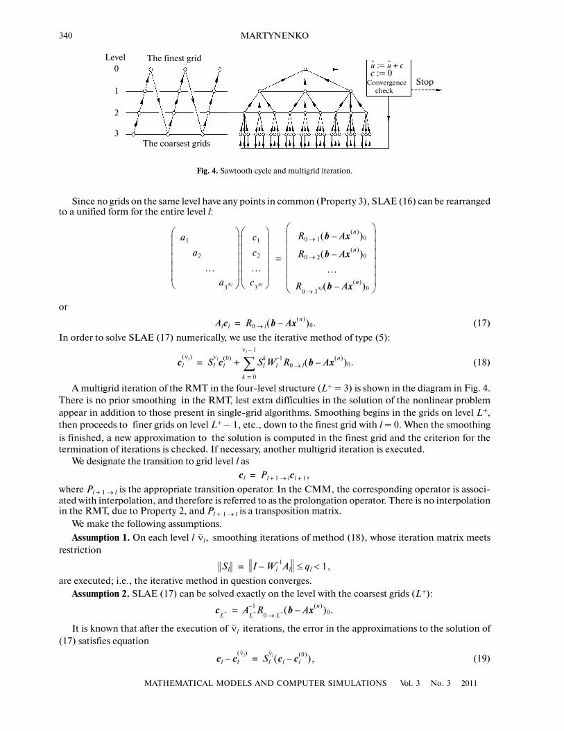
A multigrid iteration of the RMT in the four�level structure (L+ = 3) is shown in the diagram in Fig. 4.There is no prior smoothing in the RMT, lest extra difficulties in the solution of the nonlinear problemappear in addition to those present in single�grid algorithms. Smoothing begins in the grids on level L+,then proceeds to finer grids on level L+ – 1, etc., down to the finest grid with l = 0. When the smoothingis finished, a new approximation to the solution is computed in the finest grid and the criterion for thetermination of iterations is checked. If necessary, another multigrid iteration is executed.

We designate the transition to grid level l as

where Pl + 1 → l is the appropriate transition operator. In the CMM, the corresponding operator is associ�ated with interpolation, and therefore is referred to as the prolongation operator. There is no interpolationin the RMT, due to Property 2, and Pl + 1 → l is a transposition matrix.

We make the following assumptions.

Assumption 1. On each level l smoothing iterations of method (18), whose iteration matrix meetsrestriction

are executed; i.e., the iterative method in question converges.Assumption 2. SLAE (17) can be solved exactly on the level with the coarsest grids (L+):

It is known that after the execution of iterations, the error in the approximations to the solution of(17) satisfies equation

(19)

a1

a2

…a

3Nl⎝ ⎠

⎜ ⎟⎜ ⎟⎜ ⎟⎜ ⎟⎜ ⎟⎛ ⎞ c1

c2

…c

3Nl⎝ ⎠

⎜ ⎟⎜ ⎟⎜ ⎟⎜ ⎟⎜ ⎟⎛ ⎞ R0 1→ b Ax n( )–( )0

R0 2→ b Ax n( )–( )0

…

R0 3

Nl→

b Ax n( )–( )0⎝ ⎠⎜ ⎟⎜ ⎟⎜ ⎟⎜ ⎟⎜ ⎟⎜ ⎟⎛ ⎞

=

Alcl R0 l→ b Ax n( )–( )0.=

cl

νl( )Sl

νlcl0( ) Sl

kWl1– R0 l→ b Ax n( )–( )0.

k 0=

νl 1–

∑+=

cl Pl 1 l→+ cl 1+ ,=

νl,

Sl I Wl1– Al– ql 1,<≤=

cL

+ AL

+

1– R0 L

+→

b Ax n( )–( )0.=

νl

cl cl

νl( )– Sl

νl cl cl0( )–( ),=

Level The finest grid

The coarsest grids

Convergence

0

1

2

3

checkStop

u := u c+c := 0

Fig. 4. Sawtooth cycle and multigrid iteration.



where cl is the exact solution of SLAE (17),

We take the value of the correction on the previous level with coarser grids as the initial approximation

We rearrange the right side of relationship (19):

where cl + 1 is the exact solution on level l + 1:

Then,

We introduce designation

(20)

so the right�hand side of relationship (19) assumes the form

Now, relationship (19) can be rewritten in recurrent form

(21)

Next, we obtain an expression for a change in error cl – over a multigrid iteration. According to

Assumption 2, SLAE (17) can be solved exactly on the level with the coarsest grids (L+). Thus, on levelL+ – 1 with finer grids, Eq. (21) assumes the form

In view of Assumption 2 ( = ), we get

(22)

Similarly, for level L+ – 2 with still finer grids

holds, or, by virtue of (22),

where

The following relationships can be easily obtained by induction:

(23)

(24)

where dl is specified by relationship (20).

cl Al1– R0 l→ b Ax n( )–( )0.=

cl0( )

:

cl0( ) Pl 1 l→+ cl 1+

νl 1+( ).=

cl cl0( )– cl Pl 1 l→+ cl 1+

νl 1+( )– cl Pl 1 l→+ cl 1+– Pl 1 l→+ cl 1+ cl 1+

νl 1+( )–( ),+= =

cl 1+ Al 1+1– R0 l 1+→ b Ax n( )–( )0.=

cl Pl 1 l→+ cl 1+– Al1– R0 l→ Pl 1 l→+ Al 1+

1– R0 l 1+→–( ) b Ax n( )–( )0.=

dl Al1– R0 l→ Pl 1 l→+ Al 1+

1– R0 l 1+→– ,=

cl cl0( )– dl b Ax n( )–( )0 Pl 1 l→+ cl 1+ cl 1+

νl 1+( )–( ).+=

cl cl

νl( )– Sl

νldl b Ax n( )–( )0 Sl

νlPl 1 l→+ cl 1+ cl 1+νl 1+( )

–( ).+=

cl0( )

cL

+1–

cL

+1–

νL

+1–

( )

– SL

+1–

νL

+1– d

L+

1–b Ax n( )–( )0 S

L+

1–

νL

+1– P

L+

L+

1–→c

L+ c

L+

νL

+( )

–⎝ ⎠⎛ ⎞ .+=

cL

+ cL

+

νL

+( )

cL

+1–

cL

+1–

νL

+1–

( )

– SL

+1–

νL

+1– d

L+

1–b Ax n( )–( )0.=

cL

+2–

cL

+2–

νL

+2–

( )

– SL

+2–

νL

+2– d

L+

2–b Ax n( )–( )0 S

L+

2–

νL

+2– P

L+

1– L+

2–→c

L+

1–c

L+

1–

νL

+1–

( )

–⎝ ⎠⎛ ⎞ ,+=

cL

+2–

cL

+2–

νL

+2–

( )

– SL

+2–

νL

+2– d

L+

2–* b Ax n( )–( )0,=

dL

+2–

* dL

+2–

PL

+1– L

+2–→S

L+

1–

νL

+1– d

L+

1–.+=

cl cl

νl( )– Sl

νldl* b Ax n( )–( )0,=

dl*dl Pl 1 l→+ Sl 1+

νl 1+ dl 1+* , for l+ 0 1 … L+ 2,–, , ,=

AL

+1–

1– R0 L

+1–→

PL

+L

+1–→A

L+

1– R0 L

+→

, for l– L+ 1,–=⎩⎪⎨⎪⎧

=

342


MARTYNENKO

Now, it is possible to write the multigrid iteration matrix for the RMT in the case L+ ≥ 1. In the finestgrid (l = 0), Eq. (23) assumes the form

or, by virtue of c0 =

By adding x(n) to both sides, one obtains

i.e., multigrid iterations of the RMT can be written as

where M = is the iteration matrix. With respect to (24), iteration matrix M can be transformed to

By induction, one arrives at the following representation of the iteration matrix:

which results in the following estimate:

By virtue of Assumption 1, ≤ < 1, k = 0, 1, …, L+ – 1. Since is a transposition matrix,

= Cp, where Cp is a constant independent of k. Therefore, the estimate of the norm of the iter�ation matrix assumes form

The most difficult task is to obtain an estimate of ||dl||. The following assumption, termed an approximationproperty, is commonly used in the theory of multigrid methods.

Assumption 3 (the approximation property). Expression

holds, where CA is independent of l. The stated approximation property was proposed by Hackbush [5] andis conventionally employed in the proof of the convergence for diverse variants of CMM. In effect,Assumption 3 means that problems for grids on level l + 1 make good approximations to the problems forfiner grids on level l + 1 [1]. In individual cases, for instance, when solving the Dirichlet boundary valueproblem, the fact that the approximation property takes place can be proved based on the order of theaccuracy of the difference scheme [1].

With regard to Assumption 3, the estimate of the norm of iteration matrix for the RMT assumes thefinal form

(25)

c0 c0

ν0( )– S0

ν0d0* b Ax n( )–( )0,=

A01– b Ax n( )–( )0,

c0

ν0( )A0

1– S0

ν0d0*–( ) b Ax n( )–( )0 A01– S0

ν0d0*–( ) b A0x n( )–( ).= =

x n 1+( ) c0

ν0( )x n( )+ x n( ) A0

1– S0

ν0d0*–( ) b A0x n( )–( )+= =

= S0

ν0d0*A0x n( ) A01– S0

ν0d0*–( )b;+

x n 1+( ) Mx n( ) A01– S0

ν0d0*–( )b,+=

S0

ν0d0*A0

M S0

ν0d0*A0 S0

ν0 d0 P1 0→ S1

ν1d1*+( )A0 S0

ν0 d0 P1 0→ S1

ν1 d1 P2 1→ S2

ν2d2*+( )+( )A0.= = =

M S0

ν0 d0 Pk k 1–→ Sk

νkdl

k 1=

l

∏l 1=

L+

1–

∑+⎝ ⎠⎜ ⎟⎛ ⎞

A0,=

M S0


νkdl

k 1=

l

∏l 1=

L+

1–

∑+ A0⋅≤

≤ S0


νk dl⋅ ⋅k 1=

l

∏l 1=

L+

1–

∑+⎝ ⎠⎜ ⎟⎛ ⎞

A0 .

Sk

νk qk

νk Pk k 1–→

Pk k 1–→

M q0

ν0 d0 Cpkqk

νk dl

k 1=

l

∏l 1=

L+

1–

∑+⎝ ⎠⎜ ⎟⎛ ⎞

A0 .≤

dl Al1– R0 l→ Pl 1 l→+ Al 1+

1– R0 l 1+→– CA A01–,≤=

M CAq0

ν0 1 Cpkqk

νk

k 1=

l

∏l 1=

L+

1–

∑+⎝ ⎠⎜ ⎟⎛ ⎞

.≤



It follows that a sufficient number of smoothingiterations for the grids on all levels can provide||M|| < 1, i.e., ensure the convergence of theRMT. However, the obtained estimate is toorough to assess the rate of convergence. Weassume that the same number of iterations ofsome iterative method is executed in all grids forsmoothing. The amount of computational work

in the finest grid is arithmetic operations,

where is the number of points. Then, in viewof Property 2, the cost of smoothing on level l is

arithmetic operations as well. Therewith,

the cost of a multigrid iteration is (L+ + 1)arithmetic operations. Therefore, the RMTshould not be applied to accelerate the conver�gence of the iterative method in use unless thenumber of iterations required for the criterion

αN

N

αN

αN

for termination to be satisfied is much greater than the number of grid levels, ν � L+ + 1. On the other hand,

since L+ + 1 ~ the cost of a multigrid iteration in the RMT is O arithmetic operations,

which is inferior to the corresponding value O in the CMM. An extra amount of computation is aninevitable consequence of the fact that transition operators do not depend on the problem to be solved.

4. THE COMPUTATIONAL EXPERIMENT

In order to make a computational experiment, we the use the Dirichlet boundary value problem forPoisson’s equation within a unit square

(26)

that has exact solution

(27)

where

The right�hand member f(x, y) in (26) can be obtained by substitution of the exact solution (27) into theleft side of (26).

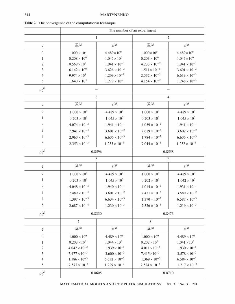
The computational experiment was performed for a six�level multigrid structure (L+ = 5) with a 1001 ×1001 finest grid (hx = hy = 1/1000), starting from an initial approximation of zero. Smoothing iterationsin each grid consisted in two combined iterations of Seidel’s method with point ordering of unknownterms.

Numerical solution of model problem (26) reduces to the solution of SLAE Ax = b. In order to estimatethe accuracy of the approximation to the solution after the qth multigrid iteration, we use the relative normof the residual vector

(28)

and the error in the approximation to the solution

(29)

The comparison of the amount of computation work requires the concept of equivalent numbers ofsmoothing iterations [2, 3]. The amount of computation work for smoothing iterations in all grids onsome level is approximately equal to the amount of computation work for smoothing iterations in the

N,log N Nlog( )

N( )

∂2u

∂x2�� ∂2u

∂y2��+ f x y,( ),–=

ua x y,( ) Q x( )Q y( ),=

Q ξ( ) 10 eξ 1 e–( )ξ 1–+( ), ξx

y⎝ ⎠⎛ ⎞ .= =

� q( ) Ax q( ) b–b

��=

ε q( ) ua xiv yj

v,( ) xijq( )– .

ijmax=

νν

Table 1. The distribution of the number of smoothing iter�ations over grid levels

The number of an experiment

l 1 2 3 4 5 6 7 8

5 1 1 1 1 1 1 1 1

4 1 1 1 1 1 1 1 1

3 1 1 1 1 1 1 1 1

2 1 1 1 1 1 2 1 2

1 1 1 1 1 2 2 3 3

0 1 2 3 4 3 3 4 4

6 7 8 9 9 10 11 12ν

344


MARTYNENKO

Table 2. The convergence of the computational technique

The number of an experiment

1 2

q �(q)ε

(q) �(q)ε

(q)

0 1.000 × 100 4.489 × 100 1.000 × 100 4.489 × 100

1 0.208 × 100 1.045 × 100 0.203 × 100 1.045 × 100

2 0.569 × 100 1.941 × 10–1 4.233 × 10–2 1.941 × 10–1

3 6.142 × 100 3.626 × 10–2 1.511 × 10–2 3.601 × 10–2

4 9.974 × 101 1.209 × 10–2 2.532 × 10–2 6.639 × 10–3

5 1.640 × 103 1.279 × 10–1 4.154 × 10–2 1.246 × 10–3

– –

3 4

q �(q)ε

(q) �(q)ε

(q)

0 1.000 × 100 4.489 × 100 1.000 × 100 4.489 × 100

1 0.203 × 100 1.045 × 100 0.203 × 100 1.045 × 100

2 4.074 × 10–2 1.941 × 10–1 4.059 × 10–2 1.941 × 10–1

3 7.941 × 10–3 3.601 × 10–2 7.619 × 10–3 3.602 × 10–2

4 2.963 × 10–3 6.635 × 10–3 1.784 × 10–3 6.635 × 10–3

5 2.353 × 10–3 1.233 × 10–3 9.044 × 10–4 1.232 × 10–3

0.8596 0.8558

5 6

q �(q)ε

(q) �(q)ε

(q)

0 1.000 × 100 4.489 × 100 1.000 × 100 4.489 × 100

1 0.203 × 100 1.045 × 100 0.202 × 100 1.042 × 100

2 4.048 × 10–2 1.940 × 10–1 4.014 × 10–2 1.931 × 10–1

3 7.489 × 10–3 3.601 × 10–2 7.421 × 10–3 3.580 × 10–2

4 1.397 × 10–3 6.634 × 10–3 1.370 × 10–3 6.587 × 10–3

5 2.687 × 10–4 1.230 × 10–3 2.526 × 10–4 1.219 × 10–3

0.8330 0.8473

7 8

q �(q)ε

(q) �(q)ε

(q)

0 1.000 × 100 4.489 × 100 1.000 × 100 4.489 × 100

1 0.203 × 100 1.044 × 100 0.202 × 100 1.041 × 100

2 4.042 × 10–2 1.939 × 10–1 4.011 ×10–2 1.930 × 10–1

3 7.477 × 10–3 3.600 × 10–2 7.415 ×10–3 3.578 × 10–2

4 1.386 × 10–3 6.632 × 10–3 1.369 × 10–3 6.584 × 10–3

5 2.577 × 10–4 1.229 × 10–3 2.524 × 10–4 1.217 × 10–3

0.8605 0.8710

ρν

q( )

ρν

q( )

ρν

q( )

ρν

q( )



finest grid. In the case under discussion, the concept of equivalent numbers of iterations makes it possibleto compare computational expenses on different levels.

We perform eight computational experiments consisting of the numerical solution of model problem(26) with a varying number of smoothing iterations. The distributions of the number of smoothing itera�tions over the grid levels and the equivalent numbers of smoothing iterations are given in Table 1.

We define the coefficient for the average reduction in the norm of the residual vector as

it indicates the average reduction in the norm of the residual vector after computations in an amount equalto the cost of smoothing iterations in the finest grid have been performed. Because x(0) = 0 in the pre�

sented experiments, the expression for coefficient assumes the form

The results of computational experiments are given in Table 2. According to estimate (25), the smooth�ing on levels with fine grids has the most impact on the rate of convergence of the RMT. One can see thatin the first and second experiments the multigrid iterations of the RMT diverge due to an insufficientnumber of smoothing iterations in the finest grid.

In the remaining experiments, the multigrid iterations of the RMT converge, and the highest rate of

convergence (the minimum value of coefficient ) is observed in the fifth experiment.

ACKNOWLEDGMENTS

This study was supported by the Russian Foundation for Basic Research, project no. 09�01�00151.

REFERENCES1. M. A. Ol’shanskii, Lectures and Exercises on Multigrid Methods (FIZMA�LIT, Moscow, 2005) [in Russian].2. S. I. Martynenko, “Robust Multigrid Technique in the Numerical Solution of Boundary Value Problems with

Structured Grids,” Vych. Met. i Prog. 1 (1), 85–104 (2000).3. S. I. Martynenko, “Robust Multigrid Technique for Black Box Software,” Comp. Meth. in Appl. Math. 6 (4),

413–435 (2006).4. S. I. Martynenko, “Robust Multigrid Technique,” Mat. Model. 21 (9), 66–79 (2009).5. W. Hackbusch, Multi�Grid Methods and Applications (Springer, Berlin, 1985).

ρν

q( ) Ax q( ) b–

Ax 0( ) b–��⎝ ⎠⎛ ⎞

1/ν

,=

ν

ρν

q( )

ρν

q( ) � q( )( )1/ν

.=

ρν

q( )

Documents

About convergence proof of robust multigrid technique