ÅBO AKADEMI - Startsidaweb.abo.fi/fak/tkf/rt/reports/rep94_3.pdf · Many routines are based on two fortran programs for linear programming, see Barrodale and Roberts (1983) and Press

ÅBO AKADEMIKEMISK-TEKNISKA FAKULTETEN

Institutionen för reglerteknik

DEPARTMENT OF CHEMICAL ENGINEERINGProcess Control Laboratory

FIN-20500, Åbo, FinlandTel.: +358 21 654 311 Fax: +358 21 654 479

l1-IDENTIFICATION TOOLBOX FOR MATLAB1

Tore K. GustafssonÅbo Akademi, Process Control Laboratory

E-mail: [email protected]

Pertti M. MäkiläLuleå University of Technology, Division of Automatic Control

E-mail: [email protected]

Version 1.1August 1994

This work was partly supported by the Academy of Finlandunder grants FA 1081195 and FA 4522

1 MATLAB is a trademark of The MathWorks, Inc.

2

Table of Contents

I Tutorial1. INTRODUCTION .................................................................................. 52. INSTALLATION .................................................................................. 53. l1-IDENTIFICATION .................................................................................. 64. MODEL STRUCTURES FOR NOMINAL MODELS.................................... 8

4.1 Fixed-Pole Models ........................................................................ 84.2 Laguerre models ........................................................................... 84.3 Kautz models ................................................................................ 94.4 Combined models........................................................................ 104.5 Model validation ......................................................................... 11

5. ESTIMATING UNCERTAINTY MODELS ................................................ 116. REFERENCES ................................................................................ 13

II Referencektz2fir ............................................................................................................ 15l1arx .............................................................................................................. 16l1fir................................................................................................................ 18l1firlgr ........................................................................................................... 19l1firud............................................................................................................ 21l1fparx ........................................................................................................... 23l1fpoe ............................................................................................................ 24l1fpoeu .......................................................................................................... 25l1fpud ............................................................................................................ 26l1fpunc........................................................................................................... 27l1kautz........................................................................................................... 28l1klt ............................................................................................................... 30lgr2fir ............................................................................................................ 32lpsimplx ......................................................................................................... 33prbs ............................................................................................................... 34rndlapl ........................................................................................................... 35

3

4

I TUTORIAL

1. INTRODUCTION

The l1-identification toolbox for Matlab (version 4) is a set of functions for approximateidentification of discrete dynamic models and estimation of uncertainty in the identifiednominal models. Most functions minimise the LSAD-criterion (Least Sum of AbsoluteDeviations) using the Simplex algorithm for Linear Programming. The formulation of theidentification problem as a linear programming problem allows inclusion of several typesof priors, and practical estimation of uncertainty.

The toolbox is available through anonymous ftp at ftp.abo.fi in directory/pub/rt/l1idtools. This toolbox must not be used for commercial purpose. The authorstake no responsibility for the correctness of the programs, nor for any inconvenience ordamage this toolbox can cause to the user. The programs may contain untested features.

Many routines are based on two fortran programs for linear programming, see Barrodaleand Roberts (1983) and Press et al. (1986). The first one, cl1app, is based on a specialisedalgorithm for l1-approximation. The second one, simplx used in lpsimplx, is a commonsimplex algorithm for linear programming. It should be noted that the function lp in theOptimization Toolbox for Matlab (Grace, 1990) is not a simplex algorithm and it is notsuitable for solving large linear programs.

Version 1.1 contains a MATLAB-language linear programming function, wlpsmplx, whichcan be used instead of the mex-function lpsimplx. The function wlpsmplx is based onfunctions wsimplex and wsimpreg, written from the interactive LP-program by HenryWolkowicz, and found at ftp.mathworks.com in directory /pub/contrib/optim/simplex1.The following gives a rule of thumb for the performance of different linear programmingfuncions. In an example with l1fpud with 200 variables, 1 inequality constraint and 92equality constraints l1fpud using lpsimplx needed 48 s, l1fpud with lpsmplx needed 226 s,and l1fpud with lp (from Optimization Toolbox) needed 1293 s CPU-time on a Sun-4.

2. INSTALLATION

Many of the routines are based on two fortran programs for linear programming. Thefortran code is supplied in f-files as well as in compiled and linked mex4-files. The mex4-files can only be used on a Sun-4 computer. The f-files must be separately compiled andlinked for other computers. The procedure is

fmex cl1app.f cl1appg.ffmex simplx.f simplxg.ffmex l1arx.f cl1app.f.

5

3. l1-IDENTIFICATION

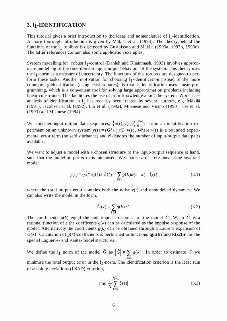
This tutorial gives a brief introduction to the ideas and nomenclature of l1-identification.A more thorough introduction is given by Mäkilä et al. (1994). The theory behind thefunctions of the l1 toolbox is discussed by Gustafsson and Mäkilä (1993a, 1993b, 1993c).The latter references contain also some application examples.

System modelling for robust l1-control (Dahleh and Khammash, 1993) involves approxi-mate modelling of the time-domain input/output behaviour of the system. This theory usesthe l1-norm as a measure of uncertainty. The functions of this toolbox are designed to per-form these tasks. Another motivation for choosing l1-identification instead of the morecommon l2-identification (using least squares), is that l1-identification uses linear pro-gramming, which is a convenient tool for solving large approximation problems includinglinear constraints. This facilitates the use of prior knowledge about the system. Worst caseanalysis of identification in l1 has recently been treated by several authors, e.g. Mäkilä(1991), Jacobsen et al. (1992), Lin et al. (1992), Milanese and Vicino (1993), Tse et al.(1993) and Milanese (1994).

We consider input-output data sequences, u t y t tt N( ), ( )k p == −

01, from an identification ex-

periment on an unknown system y t G u t v t( ) ( )( ) ( )= ∗ + , where v(t) is a bounded experi-mental error term (noise/disturbance) and N denotes the number of input/output data pairsavailable.

We want to adjust a model with a chosen structure to the input-output sequence at hand,such that the model output error is minimised. We choose a discrete linear time-invariantmodel

y t G u t t g k u t k tk

( ) ( $ )( ) ( ) ( ) ( ) ( )= ∗ + = − +≥

∑ξ ξ1

(3.1)

where the total output error contains both the noise v(t) and unmodelled dynamics. Wecan also write the model in the form,

$ ( ) ( )G z g k zk

k

=≥

∑1

(3.2)

The coefficients g(k) equal the unit impulse response of the model $G. When $G is arational function of z the coefficents g(k) can be calculated as the impulse response of themodel. Alternatively the coefficients g(k) can be obtained through a Laurent expansion of$ ( )G z . Calculation of g(k)-coefficients is performed in functions lgr2fir and ktz2fir for the

special Laguerre- and Kautz-model structures.

We define the l1 norm of the model $G as $ ( )G g kk

=≥

∑1

. In order to estimate $G we

minimise the total output error in the l1-norm. The identification criterion is the least sum

of absolute deviations (LSAD) criterion,

min ( )1

0

1

Nt

t

N

ξ=

−

∑ (3.3)

6

For some model structures it is possible to penalize the complexity of the behaviour of themodel by including a suitable weighted l1-norm of the derivative of the model in thecriterion. In the toolbox the functions for FIR-model identification can use the followingcriterion:

min ( ) ( )1

0

1

1Nt k g k

t

N

k

ξ λ=

−

≥∑ ∑+

L

NMM

O

QPP

(3.4)

The model $G, which is identified using criterion (3.3) or (3.4), is called a nominal model.A nominal model is simply the best fit to the data, without any estimates of the size orstructure of the uncertainty, which are treated later.

Model and error priors.The l1-identification functions allow the use of priors in the form of constraints. Eqn (3.3)or (3.4) is solved by linear programming, and consequently all priors which can be de-scribed as linear constraints on the adaptable parameters can be applied.

The parameter values can directly be constrained with inequality or equality constraints,

Ep f≤ (3.5)Cp d= (3.6)

where p is the parameter vector.

Smoothness priors in the form of constraints on the derivative of the transfer function ofthe identified model,

$ ( )'G k g kl

k1 11= ≤

≥∑ γ (3.7)

can be applied exactly in FIR-model identification and approximately in Laguerre- andKautz-model identification.

Constraints on the ll-gain of the identified FIR-model can be applied as

$ ( )G g kl

k1 12= ≤

≥∑ γ (3.8)

v(t) is usually in robust identification considered as a bounded noise sequence, e.g.max ( )

0 1≤ ≤ −≤

t Nv t ε . In the toolbox error priors are included as minimum and maximum val-

ues,min ( ) max ( )

0 1 0 1≤ ≤ −−

≤ ≤ −+≥ ≤

t N t Nt tξ ε ξ ε (3.9)

7

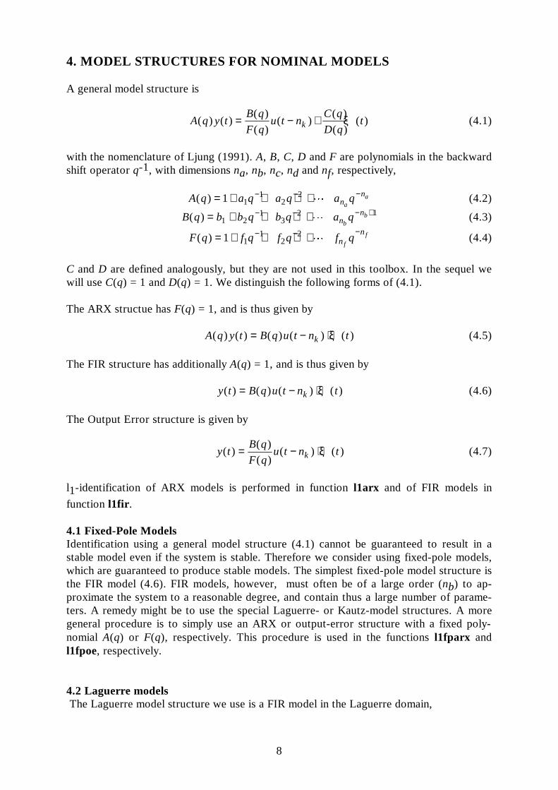
4. MODEL STRUCTURES FOR NOMINAL MODELS

A general model structure is

A q y tB q

F qu t n

C q

D qtk( ) ( )

( )

( )( )

( )

( )( )= − + ξ (4.1)

with the nomenclature of Ljung (1991). A, B, C, D and F are polynomials in the backwardshift operator q-1, with dimensions na, nb, nc, nd and nf, respectively,

A q a q a q a qnn

aa( ) = + + + +− − −1 1

12

2L (4.2)

B q b b q b q a qnn

bb( ) = + + + +− − − +

1 21

32 1L (4.3)

F q f q f q f qnn

f

f( ) = + + + +− − −1 1

12

2L (4.4)

C and D are defined analogously, but they are not used in this toolbox. In the sequel wewill use C(q) = 1 and D(q) = 1. We distinguish the following forms of (4.1).

The ARX structue has F(q) = 1, and is thus given by

A q y t B q u t n tk( ) ( ) ( ) ( ) ( )= − + ξ (4.5)

The FIR structure has additionally A(q) = 1, and is thus given by

y t B q u t n tk( ) ( ) ( ) ( )= − + ξ (4.6)

The Output Error structure is given by

y tB q

F qu t n tk( )

( )

( )( ) ( )= − + ξ (4.7)

l1-identification of ARX models is performed in function l1arx and of FIR models in

function l1fir .

4.1 Fixed-Pole ModelsIdentification using a general model structure (4.1) cannot be guaranteed to result in astable model even if the system is stable. Therefore we consider using fixed-pole models,which are guaranteed to produce stable models. The simplest fixed-pole model structure isthe FIR model (4.6). FIR models, however, must often be of a large order (nb) to ap-proximate the system to a reasonable degree, and contain thus a large number of parame-ters. A remedy might be to use the special Laguerre- or Kautz-model structures. A moregeneral procedure is to simply use an ARX or output-error structure with a fixed poly-nomial A(q) or F(q), respectively. This procedure is used in the functions l1fparx andl1fpoe, respectively.

4.2 Laguerre models The Laguerre model structure we use is a FIR model in the Laguerre domain,

8

y t B q u t tL( ) ( , ) ( ) ( )= +α ξ (4.2.1)

with the definition

B q b L q b L q b L qL n nL L( , ) ( , ) ( , ) ( , )α α α α= + + +1 1 2 2 L (4.2.2)

where Lk is the discrete Laguerre polynomial of order k,

L qq

q

q

qk

k

( , )α αα

αα

= −−

−−

F

HGI

KJ−

−

−

−

−1 2

1

1

1

11

1 1(4.2.3)

The Laguerre parameter α, |α| ≤ 1, is selected based on prior knowledge about the system,or it can be adjusted during the identification procedure. With α selected, the model(4.2.1) is a fixed-pole ARX model with multiple poles at α. The Laguerre parameter canbe seen as a time-scaling parameter, which is used in order to reduce the number ofparameters compared to a FIR model. Laguerre-model identification is performed infunction l1firlgr .

During identification of Laguerre models, the model (4.2.1) is transferred into state spaceform

x Fx G

Bx

( ) ( ) ( )

( ) ( ) ( )

t t u t

y t t t

+ = += +

1

ξ(4.2.4)

where B is a row vector of Laguerre coefficients. The state space model (4.2.4) is in thetoolbox function initialised with x(0) = 0, and simulated for a number of time intervals inorder to let the state vector converge. A part of the input/output data pairs is thus usedfor initialisation and cannot be used in the LSAD minimisation. The number of in-put/output data pairs which must be used for initialisation depends on the selected value α.

4.3 Kautz modelsThe Kautz model structure is a modified form of the Laguerre structure with a complexparameter (Wahlberg, 1991)

y t B q u t tK( ) ( , ) ( ) ( )= +α ξ (4.3.1)

with the definition

B q b q b q b qK n nK K( , ) ( , ) ( , ) ( , )α α α α= + + +1 1 2 2Ψ Ψ ΨL (4.3.2)

where Ψ k is the k:th base function,

9

Ψ

Ψ

2 1 1

1 2

1 2

1 2

1 2

1

2 2

2

1 2

1 2

1 2

1

1 1

1

1 1

1 1

1

1 1

1 2 2

j

j

j

j

K

q Caq q

b c q cq

c b c q q

b c q cq

q Cq

b c q cq

c b c q q

b c q cq

j n

−

− −

− −

− −

− −

−

−

− −

− −

− −

−

= − ++ − −

− + − ++ − −

F

HGI

KJ

=+ − −

− + − ++ − −

F

HGI

KJ

=

( , )( )

( )

( )

( , )( )

( )

( )

, , , /

α

α

K

(4.3.3)

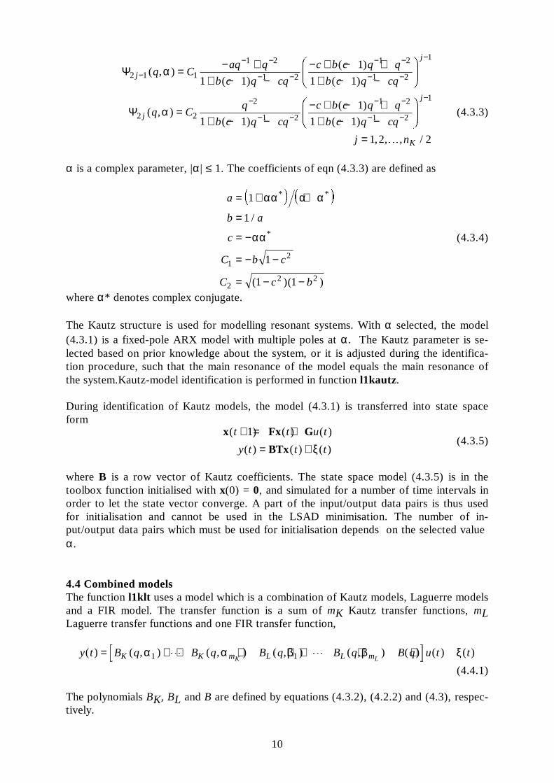
α is a complex parameter, |α| ≤ 1. The coefficients of eqn (4.3.3) are defined as

a

b a

c

C b c

C c b

= + +

=

= −

= − −

= − −

1

1

1

1 1

12

22 2

αα α α

αα

* *

*

/

( )( )

d i d i

(4.3.4)

where α* denotes complex conjugate.

The Kautz structure is used for modelling resonant systems. With α selected, the model(4.3.1) is a fixed-pole ARX model with multiple poles at α. The Kautz parameter is se-lected based on prior knowledge about the system, or it is adjusted during the identifica-tion procedure, such that the main resonance of the model equals the main resonance ofthe system.Kautz-model identification is performed in function l1kautz.

During identification of Kautz models, the model (4.3.1) is transferred into state spaceform

x Fx G

BTx

( ) ( ) ( )

( ) ( ) ( )

t t u t

y t t t

+ = += +

1

ξ(4.3.5)

where B is a row vector of Kautz coefficients. The state space model (4.3.5) is in thetoolbox function initialised with x(0) = 0, and simulated for a number of time intervals inorder to let the state vector converge. A part of the input/output data pairs is thus usedfor initialisation and cannot be used in the LSAD minimisation. The number of in-put/output data pairs which must be used for initialisation depends on the selected value α.

4.4 Combined modelsThe function l1klt uses a model which is a combination of Kautz models, Laguerre modelsand a FIR model. The transfer function is a sum of mK Kautz transfer functions, mLLaguerre transfer functions and one FIR transfer function,

y t B q B q B q B q B q u t tK K m L L mK L( ) ( , ) ( , ) ( , ) ( , ) ( ) ( ) ( )= + + + + + + +α α β β ξ1 1L L

(4.4.1)

The polynomials BK, BL and B are defined by equations (4.3.2), (4.2.2) and (4.3), respec-tively.

10

During identification of combined models, the model (4.4.1) is transferred into state spaceform

x Fx G

Bx

( ) ( ) ( )

( ) ( ) ( )

t t u t

y t t t

+ = += +

1

ξ(4.4.2)

The state space model (4.4.2) is in the toolbox function initialised with x(0) = 0, andsimulated for a number of time intervals in order to let the state vector converge. A part ofthe input/output data pairs is thus used for initialisation and cannot be used in the LSADminimisation. The number of input/output data pairs which must be used for initialisationdepends on the selected values α and β.

4.5 Model validationModel validation is used to check the identified nominal model on another set of data.Some functions, which use state models as model structures (l1firlgr, l1kautz and l1klt)perform an automatic model validation on the rest of the given data sequence, which hasnot been used for estimation. The result from the model validation is the average absoluteprediction error,

RN

tvalval

= ∑1 ξ( )validation set

(4.5.1)

This value can be compared to the average prediction error in the estimation,

RN

tid = ∑1 ξ( )estimation set

. (4.5.2)

5. ESTIMATING UNCERTAINTY MODELS

We consider uncertainty models of the form

y t G G u t t( ) ( $ ) ( ) ( )= + ∗ +∆ ξ (5.1)

We test the feasibility of an uncertainty model by testing that eqn (5.1) holds for t ∈ {avalidation set}, for some ∆G satisfying ∆G N≤ ρ( ) and for some bounded ξ(t) such that

1 N tt

ξ ε( )∑ ≤ . This procedure is followed in the function l1firud for a time varying un-

certainty, ∆G(t), of FIR structure. The uncertainty model in function l1firud is

y t B q B t q u t n tk( ) ( ) ( , ) ( ) ( )= + − +∆ ξ (5.2)

where B(q) contains the nominal model.

The actual computational procedure of function l1firud is the following: given a nominalmodel B(q) (and nk) and a value ρ we minimise the LSAD criterion (3.3) with respect to∆B t q( , ) and ξ(t). l1firud uses piece-wise constant values for ∆B t q( , ) .

11

The procedure is more closely described by Gustafsson and Mäkilä (1993a, 1993b), wherealso an example is given.

Another procedure is described by Gustafsson and Mäkilä (1993b) and Mäkilä et al(1994), and realised in function l1fpunc. Here the uncertainty model is of a fixed-poleARX-model structure,

A q y t B q u t B q u t n t t Nk( ) ( ) ( ) ( ) ( ) ( ) ( ), , , ,= + − + = −∆ ξ 0 1 1K (5.3)

where A is given as a fixed polynomial and B is the identified nominal B-polynomial. Thesize of ∆B is estimated by the following procedure, where the order of ∆B q( ) is given, m,and nk is given,

κ ε

ξ ε

( , , ) max ( )

( ) .

( )m N B q

t

B q

t

N

=

≤=

−∑

∆∆

such that eqn (5.3) is satisfied and

1

N 0

1

(5.4)

The quantity κ ε( , , )m N can be interpreted as the maximal unfalsified value of ∆B withinthe chosen uncertainty structure. The procedure involves the solution of 2m linear pro-grams, and can thus be very demanding in computer resources for larger m.

The same procedure is used in function l1fpoeu for an uncertainty model of output errorstructure,

y tB q

F qu t

B q

F qu t n t t Nk( )

( )

( )( )

( )

( )( ) ( ), , , , .= + − + = −∆ ξ 0 1 1K (5.5)

We consider the problem (5.4) to be a procedure for black-box estimation of uncertainty,that is for estimating uncertainty without prior knowledge of ε. We calculate κ ε( , , )m Nfor different values of m and ε, and plot κ ε( , , )m N as functions of m and ε. With ε biggerthan the actual value, κ ε( , , )m N should be linearly increasing with ε, but at values of ε lessthan the actual value κ ε( , , )m N decreases rapidly. An estimate of κ ε( , , )m N is thusobtained at a point where the κ-curve turns into a straight line.

A tight lower limit is given by

κ κ εε

∗ ≡( , ) inf ( , , )m N m N (5.6)

where the infimum is taken over all ε > 0 such that the constraints (5.3) and (5.4) holds.The quantity κ∗( , )m N is conveniently calculated by minimising the LSAD criterion (3.3)with respect to ∆B q( ) and ξ( )t for the model (5.3). This is the same procedure as used infunction l1firud for an uncertainty model (5.2). The corresponding function l1fpudcalculates (5.6) for the fixed-pole model (5.3) with a time invariant uncertainty.

12

Example. We have simulated a system with transfer function G z z z( ) ( . ) /= −2 1 40 2

( . . )1 1 40 0 482− +z z , with v t( )k p beeing a realisation of Gaussian white noise with variance0.02, and u t( )k p beeing a PRBS signal of unit amplitude. A nominal model (4.7) was esti-mated using l1fpoe with F(q) = 1 - 0.8q-1, which gave the model a pole equal to thedominating pole of the system. With nb = 2, nk = 1 and N = 100 we obtained for a specificsimulation run B q q q( ) . .= −− −2 0967 0 37051 2. Writing G z B z F z( ) ( ) ( )= , we get the size ofthe model error expressed in the form of the uncertainty model (5.3) as ∆B = 0 5672. .

κ-values were then estimated for m = 4, 6, 8 with function l1fpunc, using both the samedata as used un the estimation of the nominal model, and validation data with N = 100.The results are presented in Figure 1. In the figure the plots for the data used also in theestimation of the nominal model are indicated in solid. The true averages (E) of the abso-lute values of the noise v(t) are also indi-cated for the two data sets. Furthermore,κ∗-values calculated with l1fpud are indi-cated with circles. The results indicate thateven κ∗( , )m N estimates the size of theuncertainty (error) in B remarkably wellfor m = 6, 8. For m = 4 there is still con-siderable unmodelled dynamics outside thechosen uncertainty structure, and so in thiscase κ∗ underestimates the true errormore clearly. Note that the steepness ofthe curves varies in a systematic manner.

0.14 0.16 0.18 0.2 0.22 0.24 0.260.2

0.4

0.6

0.8

1

1.2

1.4

1.6

1.8

ε

κ

m=8m=8

m=6

m=6 m=4m=4

||∆B||

E E

Clearly random effects start to influencemore at the last steep part of the curves.

Figure 1. κ-values as functions of ε.

Thus the plots allow us to make a realistic choice of the size of the modelling uncertainty.

6. REFERENCES

Barrodale, I. and F.D.K. Roberts (1978). An efficient algorithm for discrete l1 linear ap-proximation with linear constraints, SIAM J. Numer. Anal., 15, 603-611.

Dahleh, M.A. and M.H. Khammash (1993). Controller design for plants with structureduncertainty, Automatica, 29, 37-56.

Grace, A. (1990). Optimization Toolbox User's Guide, The MathWorks, Inc.

Gustafsson, T.K. and P.M. Mäkilä (1993a). Modelling of uncertain systems via linear pro-gramming, Proceedings 12th IFAC World Congress, Sydney, Australia.

Gustafsson, T.K. and P.M. Mäkilä (1993b). Modelling of uncertain systems via linearprogramming, Report 93-6, PCL, Åbo Akademi University.

13

Gustafsson, T.K. and P.M. Mäkilä (1993c). On system identification and model validationvia linear programming, Proceedings 32nd IEEE Conf. on Decision and Control,San Antonio, Texas.

Mäkilä, P.M., J.R. Partington and T.K. Gustafsson (1994). Robust identification.(Tutorial paper), Preprints 10th IFAC Symp. System Identification, Vol. 1, Copen-hagen.

Jacobson, C.A., C.N. Nett and J.R.Partington (1992). Worst case system identification inl1: optimal algorithms and error bounds, Systems Control Lett., 19, 419-424.

Lin, L., L.Y.Wang and G. Zames (1992). Uncertainty principles and identification n-widths for LTI and slowly varying systems, Proceedings American Control Conf.,Chicago.

Ljung, L. (1991). System Identification Toolbox User's Guide, The MathWorks, Inc.

Mäkilä, P.M. (1991). Robust identification and Galois sequences, Int. J. Control, 54,1189-1200.

Mäkilä, P.M, J.R. Partington and T.K. Gustafsson (1994). Robust identification, 10thIFAC Symposium on Systems Identification, Copenhagen, Denmark.

Milanese, M. (1994). Worst-case l1 identification, preprint.

Milanese, M. amd A. Vicino (1993). Information based complexity and nonparametricworst-case system identification, Jour. of Complexity, 9, 427-446.

Press, W.H., B.P. Flannery, S.A. Teukolsky and W.T. Vetterling (1986). Numerical reci-pes, Cambridge University Press.

Tse, D.N.C., M.A. Dahleh and J.N. Tsitsiklis (1993). Optimal asymptotic identificationunder bounded disturbances. IEEE Trans. Automat. Control, 38, 1176-1190.

Wahlberg, B. (1991). Identification of resonant systems using Kautz filters, Proceedings30th IEEE Conf. Decision and Control, Brighton, UK.

14

II REFERENCE Version 1.1, August 25, 1994

ktz2fir

PurposeExpand a Kautz model into a truncated FIR model.

SynopsisB = ktz2fir(BK, alpha, n)

DescriptionThe Kautz model, eqn (4.3.1), is approximated by a FIR model, eqn (4.6).

BK is a row vector of Kautz coefficients, BK = b b bnK1 2 K .

alpha is the complex Kautz parameter, α α∈ <C, 1. n is the order of theresulting FIR model.

The result is the row vector of FIR coefficients, B = b b bn1 2 K , with nk = 0.

15

l1arx

PurposeEstimate the parameters of an ARX or AR model minimising the l1 norm of theprediction error.

Synopsis[A, B, stat, epsil, err, it, res] = l1arx(yu, nn, epsilon, [E f], [C d])

DescriptionThe estimated model is of a single output, multiple input ARX structure,

A q y t B q u t n B q u t n tk n n knu u u( ) ( ) ( ) ( ) ( ) ( ) ( )= − + + − +1 1 1 L ξ

with the A- and B-polynomials defined by eqs(4.2-3). The minimisation criterion is the LSAD criterion, eqn (3.3).

yu contains the output-input data, yu = [y u], where y is a column vector containing y(t) for t = 0, 1, ..., N-1. u is a matrix with input sequences as columns,

u = u unu1 K .

nn defines the orders of polynomials A and B, and the delays associated with each

input, nn = n n n n na b bn k knu u1 1L L .

epsilon = ε ε− + are the error priors, eqn (3.9). If no constraints are applied epsilon should be given the value [0 0].

[E f] and [C d] define inequality (Ex≤≤f) and equality constraints (Cx=d), where x isthe parameter vector,

x = − −a a b b b b b bn n n n n n

T

a b b u u bnu1 11 1 2 1 2 11 2L L L L L, , , , , ,

The result is given in A and B:

A = 1 1 2a a anaL

B =

L

N

MMMM

O

Q

PPPP

0 0 0 00 0 0 0

0 0 0 0

1 11 1 2 1

1 2 2 1 2 2 2

1 1 2

1 1

2

L L L

L L L

M O M M M O M M O M

L L L

n n

nk n

n n n n n

k b

b

knu u u u bnu

b b bb b b

b b b

, , ,

, , ,

, , ,

.

stat indicates the status of the result:stat=0: optimal solution foundstat=1: no feasible solution foundstat=2: calculations terminated prematurely due to rounding errorsstat=3: maximum number of iterations reached.

16

epsil = $ $ε ε− + returns an error estimate, min ( )$ max ( ) $,t t

t tξ ε ξ ε≥ ≤− + .

err returns the value of the criterion function, it returns the number of iterations and res returns the residual vector,

res=

−−−

− −− −

L

N

MMMM

O

Q

PPPP+

−

y yd Cxf Ex

y yy y

$

( $ )( $ )ε

ε

NoteThe exact number of data used for identification is

N n ni

kij

bj= − +RST

UVW

+dim( max maxy) 1.

17

l1fir

PurposeEstimate the parameters of a FIR model minimising the l1 norm of the prediction

error.

Synopsis[B, FPE, stat, epsil, l1norm, err, it] = l1fir(yu, nn, epsilon, [E f], [C d], lambda,

gamma1, gamma2)Description

The estimated model is of a FIR structure, eqn(4.6) The minimisation criterion is the augmented LSAD criterion, eqn (3.4).

yu contains the output-input data, yu = [y u], where y and u are column vectors containing y(t) and u(t) for t = 0, 1, ..., N-1.

nn = n nb k .


[E f] and [C d] define inequality (Ex≤≤f) and equality constraints (Cx=d), where x is

the parameter vector, x = b b bnT

b1 2 L .

lambda is the weight factor (λ) of eqn (3.4), gamma1 and gamma2 are the constraints γ1 and γ2 of eqns (3.7) and (3.8), respectively. gamma1 ≤ 0 and gamma2 ≤ 0 imply no constraints.

The result is given in B = 0 0 1 2L Lb b bnb, with the first nk elements

zero.

FPE is Akaike's Final Prediction Error (Ljung, 1991).


epsil = ε ε− + returns an error estimate, min ( )$ max ( ) $,t t

t tξ ε ξ ε≥ ≤− + .

l1norm is the averaged one-step ahead prediction error, l1norm= −y y$ 1 N.

err returns the value of the criterion function and it returns the number of iterations.The exact number of data used for identification, N n nk b= − + +dim(y) b g 1.

18

l1firlgr

PurposeEstimate the parameters of a FIR model in the Laguerre domain minimising the l1norm of the prediction error. l1firlgr performes also a model validation.

Synopsis[Bl, FPE, stat, epsil, l1norm, l1val, err, it] = l1firlgr(yu, nn, alpha, t0, nt, epsilon,

[E f], [C d], gamma1)Description

The estimated model is of a FIR structure in the Laguerre domain, eqns (4.2.1) to(4.2.3). The minimisation criterion is the LSAD criterion, eqn (3.3).

Matrix yu contains the output-input data, yu = [y u], where y and u are columnvectors containing y(t) and u(t) for t = 0, 1, ..., N-1.

nn = 0 nL . alpha is the Laguerre parameter α, α <1.

t0 denotes the first data pair (y, u) to be used for identification. Data pairsy u( ), ( )1 1k p to y t u t( ), ( )0 01 1− −l q are used to let the state space form (4.2.4) of the

Laguerre model approximately converge to the correct state before starting the es-timation procedure.

nt is the number of data pairs used for identification.

epsilon = ε ε− + are the error priors, eqn (3.9). If no constraints are appliedepsilon should be given the value [0 0].

[E f] and [C d] define inequality and equality constraints, which are not imple-mented in this version.

gamma1 is the constraint γ1 of eqn (3.7). gamma1 ≤ 0 implies no constraint.

The result is given in Bl = b b bnL1 2 L .




t tξ ε ξ ε≥ ≤− + .

l1norm is the averaged one-step ahead prediction error, l1norm= = −R Nid y y$ 1 ,

where N = nt.

19

l1val returns the averaged l1 norm of the prediction error, l1val = Rval =y y− − − −$ ( )1 0 1n t nt ,for the model validation data set,

y t n u t nt t( ), ( )0 01 1+ + + +l q to y n u n( ), ( )k p, where n is the total length of the times

series y(t) and u(t).

err returns the value of the criterion function and it returns the number of iterations.

20

l1firud

PurposeEstimate the parameters of a FIR model minimising the l1 norm of the predictionerror. Take slowly time-varying unmodelled dynamics into consideration.

Synopsis[B, FPE, stat, epsil, l1norm, err, it, Delta] = l1firud(yu, nn, epsilon, [E f], [C d],

lambda, gamma1, gamma2, kappa, ndelta, tdelta)Description

The estimated model is of a FIR structure, eqn (5.2). The minimisation criterion is the augmented LSAD criterion, eqn (3.4).

Only the first lefthand argument and two first righthand arguments are obligatory.

Matrix yu contains the output-input data, yu = [y u], where y and u are column vectors containing y(t) and u(t) for t = 0, 1, ..., N-1. nn = n nb k .




b1 2 L .

lambda is the weight factor (λ) of eqn (3.4), gamma1 and gamma2 are the constraints γ1 and γ2 of eqns (3.7) and (3.8), respectively. gamma1 ≤ 0 and gamma2 ≤ 0 imply no constraints.

kappa is a constraint (κ) on the l1-norm of the unmodelled dynamics,

δ κδ

ii

n

t t N( ) , ,=∑ ≤ ∀ ∈ −

1

0 1 1Kk p

where δi are the coeficients of the polynomial ∆B t q( , ), and nδ = ndelta is the orderof the unmodelled dynamics.

tdelta (tδ ) is the length of the time periods with constant unmodelled dynamics. The unmodelled dynamics is identified as a set of piece-wise constant polynomials for time periods of length tδ , 1≤ ≤t Nδ .

∆ ∆B t q B q i n t i t i ti t( , ) ( ), , , , ( ) , ,= = = − ⋅ + ⋅1 1 1K Kδ δ .The last period can be shorter than tδ . N is the total number of values in the time series used for identification and nt is defined as ceil(N tδ ).

N y n n nk b= − −dim( ) max( , )δ . If tdelta is greater than N, then tδ = N is used.


zero.

stat indicates the status of the result:

21

stat=0: optimal solution foundstat=1: no feasible solution foundstat=2: calculations terminated prematurely due to rounding errorsstat=3: maximum number of iterations reached.


t tξ ε ξ ε≥ ≤− + .


err returns the value of the criterion function and it returns the number of iterations.

Delta returns the coefficients of the unmodelled dynamics in the form of a matrix where the nk leftmost elements are zero,

Delta=

L

N

MMMM

O

Q

PPPP

0 00 0

0 0

11 1

2 1 2

1

L L

L L

M O M M O M

L L

δ δδ δ

δ δ

δ

δ

δ

, ,

, ,

, ,

n

n

n n nt t

.

AlgorithmNote that the estimation of unmodelled dynamics can be computationally very de-manding. The vector of parameters to be estimated will be dim(x) = n n nb t+ 2 δ andthe number of inequalities will be dim(f ') = dim( )f + +3n n nt tδ . The epsilon con-straint will still increase the dimension of the inequalities with 2N. The lambda co-efficient will increase the dimension of the equalities with nb. The gamma1 con-straint will increase the dimension of the estimation vector with nb and the dimen-sion of the inequalities with 3 1nb + . The gamma2 constraint will also increase thedimension of the estimation vector with nb and the dimension of the inequalitieswith 3 1nb + .

22

l1fparx

PurposeEstimate the parameters of a fiexed-pole ARX model minimising the l1 norm of theprediction error.

Synopsis[B, FPE, stat, epsil, l1norm, err, it] = l1fparx(yu, nn, A, epsilon, [E f], [C d])

DescriptionThe estimated model is of an ARX structure, eqn (4.5) with a given fixed A-polynomial. The minimisation criterion is the LSAD criterion, eqn (3.3).

Only the first lefthand argument and the two first righthand arguments are obligatory.

matrix yu contains the output-input data, yu = [y u], where y and u are column vectors containing y(t) and u(t) for t = 0, 1, ..., N-1.

nn = n nb k .

A is a row vector containing the coefficients of the apriori given polynomial A q( ),with the first element equal to one.




b1 2 L .


zero.



t tξ ε ξ ε≥ ≤− + .


err returns the value of the criterion function and it returns the number of iterations.The exact number of data used for identification, N = dim(y) - max ,n n na k b− + −1 1l q.

23

l1fpoe

Purpose:Estimation of the parameters of a fixed-pole Output Error model using l1-approxi-mation.

Synopsis:[B, FPE, stat, epsil, l1norm, err, it] = l1fpoe(yu, nn, F, epsilon, [E f], [C d])

Description:The identification model is of the OE-model structure, eqn (4.7), with a given fixedF-polynomial. The minimisation criterion is the LSAD criterion (3.3).

Only the first lefthand and the two first righthand arguments are obligatory.

Matrix yu contains the output-input data yu=[y u], where y and u are columnvectors. nn is given as

nn = n nb k .

F is a row vector containing the coefficients of the given polynomial F q( ), with thefirst element equal to one.

epsilon = ε ε− + are apriori given minimum and maximum constraints on thedisturbance, eqn (3.9). epsilon can be set to [0 0] if no constraints should be applied.



b1 2 L .

The result is stored in the row vector B, with nk+nb columns and with the first nkelements equal to zero,

B = 0 0 1 2L Lb b bnb.

stat indicates the status of the result:stat=0: optimal solution foundstat=1: no feasible solutionstat=2: calculations terminated prematurely due to rounding errorsstat=3: maximum number of iterations reached.

The maximum number of iterations is set to 500.

epsil returns an estimate of the minimum and maximum value of the disturbance. Theformat is epsil = $ $ε ε− + .

l1norm returns the average of the absolute prediction error, that is l1norm =y y− $

1 N .

err returns the value of the criteria function and it returns the number of iterations.

24

l1fpoeu

Purpose:Estimation of uncertainty models for fixed-pole Output Error nominal models.

Synopsis:[kappa, DeltaB, P, LPlog] = l1fpoeu(yu, nn, F, B, epsil, trace)

Description:The uncertainty model is of output error type, eqn (5.5). The algorithm estimates thesize of ∆B q( ) as the maximum unfalsified value, κ ε( , , )m N for a given order of∆B q( ) , according to the procedure (5.4) with respect to the model (5.4) instead of(5.3).

Matrix yu contains the output-input data yu = [y u], where y and u are column vec-tors containing y(t) and u(t) for t = 0, 1, ..., N-1. nn is given as nn = [m nk] where mdefines the order of ∆B q( ) and nk defines the time delay associated with the input.

F is a row vector containing the coefficients of the polynomial F q( ), with the firstelement equal to one. B is a row vector containing the coefficients of the polyno-mial B q( ) . Normally the first element of B is zero. epsil is the constraint ε on thenoise in equation (5.4).

trace = 1 gives an intermediate result after each of the 2m maximisations. trace = 0suppresses intermediate output.

The output variables are kappa = κ ε( , , )m N . DeltaB is a row vector containing thecoefficients of the polynomial ∆B q( ) , which gives a maximum κ ε( , , )m N . P is an(m, 2)-matrix giving the minimum and maximum values for each coefficient of ∆B q( )from the 2m linear programs. LPlog is a column vector with 2m entries, describingthe state of each linear program, 0 means that maximum is achieved, -1 means infea-sibility and 1 means unboundness.

AlgorithmThe maximisation problem is decomposed into 2m standard linear programmingproblems, which are solved using the routine lpsimplx.

25

l1fpud

PurposeEstimate a lower limit κ∗, eqn (5.6), for the size of the uncertainty, according tothe ARX uncertainty model of equation (5.3). The nominal model is to be given.

Synopsis[epsil, kappa, DeltaB, LPlog] = l1fpud(yu, nn, A, B)

DescriptionMatrix yu contains the output-input data, yu = [y u], where y and u are column vectors containing y(t) and u(t) for t = 0, 1, ..., N-1. nn = m nk .

A is a row vector containing the coefficients of the polynomial A q( ), with the firstelement equal to one. B is a row vector containing the coefficients of thepolynomial B q( ) , with the first element equal to zero. A and B defines the nominalmodel .

epsil is the value of the LSAD criterion (3.3), that is the value of ε which gives theinfinum of eqation (5.6).

kappa is the resulting value κ∗( , )m N , equation (5.6).

DeltaB gives the resulting coefficients of ∆B q( ) , DeltaB= δ δ δ1 2 L m , with

the first element nonzero.

LPlog describes the state of the linear program, 0 means that minimum is achieved,-1 means infeasibility and 1 means unboundness.

26

l1fpunc

PurposeEstimation of uncertainty models for fixed-pole ARX nominal models.

Synopsis[kappa, DeltaB, P, LPlog] = l1fpunc(yu, nn, A, B, epsil, trace)

Description:The uncertainty model is of ARX structure, equation (5.3). The algorithm estimatesthe size of ∆B q( ) as the maximum unfalsified value, κ ε( , , )m N for a given order of∆B q( ) , according to the procedure (5.4).

Matrix yu contains the output-input data yu = [y u], where y and u are column vec-tors containing y(t) and u(t) for t = 0, 1, ..., N-1. nn is given as nn = [m nk] where mdefines the order of ∆B q( ) and nk defines the time delay associated with the input.

A is a row vector containing the coefficients of the polynomial A q( ), with the firstelement equal to one. B is a row vector containing the coefficients of the polyno-mial B q( ) . Normally the first element of B is zero. A and B defines the nominalARX model.

epsil is the constraint ε on the noise in equation (5.4).

trace=1 gives an intermediate result after each of the 2m maximisations. trace=0suppresses intermediate output.

The output variables are kappa = κ ε( , , )m N . DeltaB is a row vector containing thecoefficients of the polynomial ∆B q( ) , which gives a maximum κ ε( , , )m N . P is an(m, 2)-matrix giving the minimum and maximum values for each coefficient of ∆B q( )from the 2m linear programs. LPlog is a column vector with 2m entries, describingthe state of each linear program, 0 means that maximum is achieved, -1 means infea-sibility and 1 means unboundness.

Algorithm:The maximization problem above is decomposed into 2m standard linear program-ming problems, which are solved using the routine lpsimplx.

27

l1kautz

PurposeEstimate the parameters of a discrete Kautz model minimising the l1 norm of theprediction error. l1kautz performes also a model validation.

Synopsis[Bk, FPE, stat, epsil, l1norm, l1val, err, it, FGH] = l1kautz(yu, nn, alpha, t0, nt,

epsilon, [E f], [C d], gamma1)Description

The estimated model is of a Kautz structure, eqns (4.3.1) to (4.3.4). The minimisa-tion criterion is the LSAD criterion, eqn (3.3).


nn = 0 nK . alpha is the complex Kautz parameter α, α <1.

t0 denotes the first data pair (y, u) to be used for identification. Data pairsy u( ), ( )1 1k p to y t u t( ), ( )0 01 1− −l q are used to let the state space form (4.3.5) of the

Kautz model approximately converge to the correct state before starting the esti-mation procedure.


epsilon = ε ε− + are the error priors, eqn (3.9). If no constraints are appliedepsilon should be given the value [0 0].

[E f] and [C d] define inequality and equality constraints, which are not imple-mented in this version.

gamma1 is the constraint γ1 of eqn (3.7). gamma1 ≤ 0 implies no constraint.

The result is given in Bk = b b bnK1 2 L .




t tξ ε ξ ε≥ ≤− + .


where N = nt.

28

l1val returns the averaged l1 norm of the prediction error, l1val = Rval =y y− − − −$ ( )1 0 1n t nt ,for the model validation data set,

y t n u t nt t( ), ( )0 01 1+ + + +l q to y n u n( ), ( )k p, where n is the total length of the times


err returns the value of the criterion function and it returns the number of itera-tions.

FGH returns the state-space model (4.3.5) in the form FGH = [F G H], where H =BT.

29

l1klt

PurposeEstimate the parameters of a combination of discrete Kautz, Laguerre and FIRmodels minimising the l1 norm of the prediction error. l1klt performes also a modelvalidation.

Synopsis[F, G, B, FPE, stat, l1norm, l1val, err, it] = l1klt(yu, nn, kautz, laguerre, t0, nt)

DescriptionThe estimated model is of a fixed-pole state space structure, eqn (4.4.2), with aspecial selection of poles according to equation (4.4.1). The minimisation criterionis the LSAD criterion, eqn (3.3).


nn = n n nK L b , where nK is the even order of the Kautz polynomials, nL is the

order of the Laguerre polynomials and nb is the order of the FIR polynomial (seeequations (4.3.2), (4.2.2) and (4.3), respectively.

kautz is a column vector of complex Kautz parameters α αi i Ki m, ,< =1 1K .

laguerre is a column vector of real Laguerre parameters β βi i Li m, ,< =1 1K .

t0 denotes the first data pair (y, u) to be used for identification. Data pairsy u( ), ( )1 1k p to y t u t( ), ( )0 01 1− −l q are used to let the state space model (4.4.2) ap-

proximately converge to the correct state before starting the estimation procedure.


The identified state model (4.4.2) is stored in matrices F, G and B.




where N = nt.

l1val returns the averaged l1 norm of the prediction error, l1val = Rval= y y− − − −$ ( )1 0 1n t nt , for the model validation data set,

30

y t n u t nt t( ), ( )0 01 1+ + + +l q to y n u n( ), ( )k p, where n is the total length of the time


err returns the value of the criterion function and it returns the number of itera-tions.

31

lgr2fir

PurposeExpand a Laguerre model into a truncated FIR model.

SynopsisB = lgr2fir(BL, alpha, n)

DescriptionThe Laguerre model, eqn (4.2.1), is approximated by a FIR model, eqn (4.6).

BK is a row vector of Laguerre coefficients, BL = b b bnL1 2 K .

alpha is the real Laguerre parameter, α <1.n is the order of the resulting FIR model.

The result is the row vector of FIR coefficients, B = b b bn1 2 K , with nk = 0.

32

lpsimplx

PurposeSolves linear programming problems using the simplex algorithm.

Synopsis[x, obj, how] = lpsimplx(f, A1, b1, A2, b2, A3, b3)

Descriptionlpsimplx solves the linear programming problem

maxx

3

f x A x b

A x b

A x b x 0

T subject to

and .

n s 1 1

2 2

3

≤

=≥ ≥

where f is a vector of constant coefficients. The matrices A and vectors b are thecoefficients of the linear constraints. It is recommended (but not required) that thevectors b1, b2 and b3 contain only non negative entries. Negative entries in the b-vectors cause lpsimplx to rearrange the constraints before constructing the tableauused by the simplex algorithm.

x returns a solution to the linear problem.

obj returns the value of the objective function fTx for the obtained solution.

how returns a string indicating the state of the result. how = 0 indicates that theobtained solution is a true solution to the linear program, how = -1 indicates that theproblem is infeasible, e.g. there is no solution because of too restrictive constraints,and how = 1 indicates that the problem has an unbounded solution.

Arguments A3, b3 and A2, b2 can be omitted. Missing constraints can also beindicated with empty matrices.

AlgorithmThe algorithm is based on the implementation of the simplex method by Kuenzi, etal. [1], and is copied from the fortran version of Press et al. [2]. This routine consistsof a matlab function, lpsimplx.m, which constructs the tableau used in the programof Press et al., and a function, simplx.mex4, which is compiled from two fortranfiles, simplxg.f and simplx.f.

References[1] Kuenzi, H.P., Tzschach, H.G. and Zehnder, C.A., Numerical Methods of

Optimization, Academic Press 1971.[2] Press, W.H., Flannery,B.P., Teukolsky, S.A. and Vetterling, W.T.,

Numerical Recipes, Cambridge University Press, 1986.

33

prbs

PurposePseudo-random binary signal generator.

Synopsisy = prbs(n, mist, mast)y = prbs(n, mist, mast, F)

Descriptionprbs generates a column vector (dimension y(n,1)) with a pseudo-random sequenceof numbers +1 and -1. The period between two switches (between +1 and -1 or viceversa) is stochastic variable with an approximate exponential distribution between aminimum switching period, mist, and a maximum switching period, mast. mist andmast must be given in discrete time periods (integers).

F is an optional parameter, 0.001 ≤ F ≤ 0.999. F = 0 would imply uniform distribu-tion of switching periods between mist and mast. F = 1 would imply exponentialdistribution of switching periods between mist and mast. The default is F = 0.8.

prbs generates uniform random numbers using the MATLAB function rand. The seedof rand may be set before calling prbs.

NoteVersion 4 of Matlab allows the user to change the function rand to give normallydistributed random numbers. Make sure that rand gives uniformly distributed randomnumbers before using prbs.

34

rndlapl

PurposeLaplace-distributed random number generator.

Synopsisx = rndlaplx = rndlapl(m, n)x = rndlapl(m, n, var)

Descriptionrndlapl generates Laplace-distributed (doublesided exponential) random numbers.The probability density function is

f x eX

x( ) = ⋅

−1

2

2

σσ

where σ is the standard deviation. The expected value is 0.

rndlapl generates one random sample from the Laplace-distributed stochasticvariable with variance 1. rndlapl(m ,n) generates an m-by-n matrix with randomentries from the Laplace-distributed stochastic variable with variance 1. rndlapl(m, n,var) generates random numbers from the Laplace-distributed stochastic variable withvariance var.

Algorithmrndlapl generates Laplace-distributed random numbers by transforming uniformlydistributed random numbers , u ∈ −1 2 1 2/ / , using the inverse of the distributionfunction,

x u u= ⋅ −sign( ) ln( )σ2

1 2

rndlapl generates Laplace-distributed random numbers using the standard MATLABfunction rand combined with the shuffling routine of Bays and Durham [1]. The seedof rand may be set before calling rndlapl.

NoteVersion 4 of Matlab allows the user to change the function rand to give normallydistributed random numbers. Make sure that rand gives uniformly distributed randomnumbers before using rndlapl.

References[1] Press, W.H., B.P. Flannery, S.A. Teukolsky and W.T. Vetterling, NumericalRecipes, Cambridge University Press 1989.

35

wlpsmplx


Synopsis[x, obj, how] = wlpsmplx(f, A1, b1, A2, b2, A3, b3)

Descriptionwlpsmplx solves the linear programming problem

maxx

3

f x A x b

A x b

A x b x 0

T subject to

and .

n s 1 1

2 2

3

≤

=≥ ≥

where f is a vector of constant coefficients. The matrices A and vectors b are thecoefficients of the linear constraints. It is recommended (but not required) that thevectors b1, b2 and b3 contain only non negative entries. Negative entries in the b-vectors cause wlpsmplx to rearrange the constraints before constructing the tableauused by the simplex algorithm.


obj returns the value of the objective function fTx for the obtained solution.

how returns a string indicating the state of the result. how = 0 indicates that the ob-tained solution is a true solution to the linear program, how = -1 indicates that theproblem is infeasible, e.g. there is no solution because of too restrictive constraints,and how = 1 indicates that the problem has an unbounded solution. how = 2 indi-cates a solution with significant roundoff error and how = 3 indicates violation of theiteration bound in function wsimpreg. The iteration bound for the phase 1 and phase2 iterations are set at 10000. It can be changed in the file wsimpreg.m.

Arguments A3, b3 and A2, b2 can be omitted. Missing constraints can also be indi-cated with empty matrices.

AlgorithmThe algorithm is based on the implementation of the simplex method by HenryWolkowicz, in functions wsimplex and wsimpreg. These functions are rewrittenforms of the interactive LP program from the files main.m and reg.m, respectively, ofHenry Wolkowicz.Compared to lpsimplex, wlpsmplx is much slower (4.5 times slower in an examplewith dim(x) = 200, dim(b1) = 1, dim(b2) = 92 and dim(b3) = 0). Contrary to lpsim-plex, wlpsmplx is written completely in MATLAB language, and is thus simply port-able between computers.

See alsowsimplex, lpsimplex

36

wsimplex


Synopsis[x, obj, how, iter] = wsimplex(A, b, c, m1, m2,)

Descriptionwsimplex solves the linear programming problem

minx

c x A x b x 0o t subject to , .≤ ≥

where c is a row vector of constant coefficients. The matrix A and vector b are thecoefficients of the linear constraints. It is required that the vector b contains onlynon negative entries. The first m1 constraints are less or equal. The last m2 con-straints are equality constraints. m1 + m2 must equal the row dimension of A and b.


obj returns the value of the objective function cx for the obtained solution.

how returns a string indicating the state of the result. how = 0 indicates that the ob-tained solution is a true solution to the linear program, how = -1 indicates that theproblem is infeasible, e.g. there is no solution because of too restrictive constraints,and how = 1 indicates that the problem has an unbounded solution. how = 2 indi-cates a solution with significant roundoff error and how = 3 indicates violation of theiteration bound in function wsimpreg. The iteration bound for the phase 1 and phase2 iterations are set at 10000. It can be changed in the file wsimpreg.m.

iter returns the number of iterations performed in phase 2 (or in phase 1 if phase 2was never performed).

AlgorithmThe algorithm is based on the implementation of the simplex method by HenryWolkowicz, in functions wsimplex and wsimpreg. These functions are rewritten fromthe interactive LP program from the files main.m and reg.m, respectively, of HenryWolkowicz.Compared to lpsimplex, wsimplex is much slower (4.5 times slower in an examplewith dim(x) = 200, m1 = 1 and m2 = 92). Contrary to lpsimplex, wsimplex is writtencompletely in MATLAB language, and is thus simply portable between computers.

See alsowlpsmplx, lpsimplx

37

Documents

ÅBO AKADEMI - Startsidaweb.abo.fi/fak/tkf/rt/reports/rep94_3.pdf · Many routines are based on two fortran programs for linear programming, see Barrodale and Roberts (1983) and Press