Embed Size (px)
Citation preview

Abnormal Cardiac Beat Detection
By
HASAN ASHRAF
MUNIM REHMAN KAYANI
MUHAMMAD UMER QURESHI
DEPARTMENT OF ELECTRICAL ENGINEERING,
PAKISTAN INSTITUTE OF ENGINEERING AND APPLIED SCIENCES,
NILORE, ISLAMABAD 45650, PAKISTAN
JUNE 2015

ii

iii
Department of Electrical Engineering
Pakistan Institute of Engineering and Applied Sciences (PIEAS)
Nilore, Islamabad 45650, Pakistan
Declaration of Originality
I hereby declare that the work contained in this thesis and the intellectual content of
this thesis are the product of my own research. This thesis has not been
previously published in any form nor does it contain any verbatim of the published
resources which could be treated as infringement of the international copyright law. I
also declare that I do understand the terms copyright and plagiarism, and that
in case of any copyright violation or plagiarism found in this work, I will be held fully
responsible of the consequences of any such violation.
Name Signature
Hasan Ashraf ____________________
Munim Rehman Kayani ____________________
Muhammad Umer Qureshi ____________________
Date: ________________
Place: ________________

iv
Certificate of Approval
This is to certify that the work contained in this thesis entitled
“Abnormal Cardiac Beat Detection”
was carried out by
Hasan Ashraf
Munim Rehman Kayani
Muhammad Umer Qureshi
under my supervision and that in my opinion, it is fully adequate,
in scope and quality, for the degree of BS Electrical Engineering from
Pakistan Institute of Engineering and Applied Sciences (PIEAS).
Approved By:
Signature: ___________________________
Supervisor: Dr. Fayyaz ul Amir Afsar Minhas
Verified By:
Signature: _________________________
Head, Department of Electrical Engineering
Stamp:

v
To our parents, siblings, teachers, and colleagues
We thank you all.

vi
Acknowledgements
Praise be to Almighty Allah who bestowed upon us the mental faculties to
contemplate the universe and gave us the strength and courage to aim for and achieve
our goals.
We are very grateful to our project supervisor Dr. Fayyaz ul Amir Afsar Minhas and
our co supervisor Mr. Muhammad Shahid Nazir for their guidance and help. We are
grateful to Mr. Muhammad Shahid Nazir for arranging lab facilities to work on this
project.We must also thank Dr. Waqas Ahmed and Dr. Muhammad Tufail, our
examiners, for their time and interest.
We would like to think Mr. Jamal Afzal and Mr. Shahzad Nadeem for providing us
with laboratory facilities. Special thanks go to our colleagues Ehab ul Haq (BSEE),
Ahmad Ali (BSEE), and Shafiq Ahmed (MSSE) for their technical assistance which
has proved vital in the completion of this project.

vii
Table of Contents
Declaration of Originality ............................................................................................ iii
Certificate of Approval ................................................................................................. iv
Acknowledgements ....................................................................................................... vi
Table of Contents ......................................................................................................... vii
Table of Figures ............................................................................................................. x
Table of Tables ............................................................................................................ xii
Abstract .......................................................................................................................... 1
1 Introduction ............................................................................................................ 2
1.1 Objectives and Motivation of the project ........................................................ 2
1.2 System Architecture ........................................................................................ 2
1.2.1 Hardware Implementation ....................................................................... 3
1.2.2 Software Implementation ......................................................................... 3
1.3 Organization of the Report .............................................................................. 4
2 The Human Heart ................................................................................................... 6
2.1 Electrical Conduction System of Heart ........................................................... 6
2.1.1 Action Potentials in the Heart .................................................................. 6
2.1.2 Initiation and Propagation Action Potentials in the Heart ....................... 7
2.2 Measurement of Electrical Activity in the Heart ............................................ 8
2.3 ECG Systems................................................................................................... 8
2.3.1 The 12-Lead ECG System ....................................................................... 8
2.3.2 Three Electrode ECG System: ............................................................... 11
2.4 ECG Waveform ............................................................................................. 11
2.4.1 P Wave ................................................................................................... 11
2.4.2 QRS Complex ........................................................................................ 12
2.4.3 T Wave ................................................................................................... 12
2.4.4 U Wave .................................................................................................. 12
viii
2.4.5 PR Interval ............................................................................................. 12
2.4.6 QT Interval ............................................................................................. 13
2.4.7 ST Segment ............................................................................................ 13
3 ECG Acquisition .................................................................................................. 14
3.1 Basic Concept ................................................................................................ 14
3.1.1 Electrodes ............................................................................................... 14
3.1.2 Electrode Types ..................................................................................... 15
3.1.3 Amplifier ................................................................................................ 15
3.1.4 Filtering .................................................................................................. 17
3.2 ECG Acquisition System .............................................................................. 18
3.2.1 Instrumentation Amplifier ..................................................................... 18
3.2.2 Right Leg Drive ..................................................................................... 19
3.2.3 Filtering .................................................................................................. 19
4 Interfacing ............................................................................................................ 20
4.1 Interfacing using USB ................................................................................... 20
4.1.1 Analog to Digital Converter (ADC) ...................................................... 20
4.1.2 Universal Serial Bus (USB) ................................................................... 21
4.1.3 USB Compatible Device ........................................................................ 23
4.2 Interfacing using the Sound Card Input ........................................................ 27
4.1.4 Frequency Modulation ........................................................................... 28
4.1.5 Voltage to Frequency Converter ............................................................ 28
4.1.6 V to F converter design .......................................................................... 28
4.1.7 Interfacing with the sound card.............................................................. 31
4.1.8 Demodulation ......................................................................................... 32
4.2 Acquisition and interfacing circuitry............................................................. 33
5 Artifact Removal and QRS Complex Detection .................................................. 34
5.1 Artifact Removal ........................................................................................... 34

ix
5.1.1 ECG Artifacts......................................................................................... 34
5.1.2 Artifact Removal Techniques ................................................................ 34
5.1.3 Implementation and Results ................................................................... 36
5.2 QRS detection ............................................................................................... 37
5.2.1 The Length Transform for QRS detection ............................................. 37
5.2.2 Implementation and Results ................................................................... 38
5.3 R wave ........................................................................................................... 43
5.3.1 R peak detection ..................................................................................... 43
5.3.2 RR interval ............................................................................................. 43
6 Support Vector Machine for Abnormal Beat Detection ...................................... 45
6.1 Support Vector Machines .............................................................................. 45
6.2 One-class SVM ............................................................................................. 48
6.3 Implementation.............................................................................................. 48
6.3.1 Feature Extraction .................................................................................. 49
6.3.2 Training and Testing .............................................................................. 49
6.3.3 Evaluation .............................................................................................. 49
7 Conclusions and Future Work ............................................................................. 51
Appendix A .................................................................................................................. 53
Appendix B .................................................................................................................. 56
Appendix C .................................................................................................................. 58
Appendix D .................................................................................................................. 60
Appendix E .................................................................................................................. 65
References .................................................................................................................... 74

x
Table of Figures
Figure 1-1 Block diagram of hardware implementation ................................................ 3
Figure 1-2 Block diagram of software implementation ................................................. 4
Figure 2-1 Heart’s Conduction System [3] .................................................................... 6
Figure 2-2 Action Potentials in heart [4] ....................................................................... 7
Figure 2-3 Limb lead placement [3] ............................................................................ 10
Figure 2-4 Precordial lead placement [3]..................................................................... 10
Figure 2-5 ECG waveform [3] ..................................................................................... 11
Figure 3-1 Block Diagram of ECG Acquisition Circuit .............................................. 14
Figure 3-2 Polarizable Electrode ................................................................................. 15
Figure 3-3 Non Polarizable Electrode .......................................................................... 15
Figure 3-4 Three Operational Amplifier Differential Amplifier Topology [6] ........... 16
Figure 3-5 Block Diagram of three Lead ECG system ................................................ 18
Figure 3-6 AD620 Circuit [5] ..................................................................................... 19
Figure 3-7 Leg Drive ................................................................................................... 19
Figure 3-8 High pass and Low pass Filters .................................................................. 19
Figure 4-1 Block Diagram for USB interface .............................................................. 20
Figure 4-2 Flow chart................................................................................................... 23
Figure 4-3 Flow diagram for Main Method ................................................................. 24
Figure 4-4 Flow Diagram for the Save_File Method................................................... 25
Figure 4-5 Flow Diagram for the Acquire_Data Method ............................................ 25
Figure 4-6 Flow Diagram for the Stream Method ...................................................... 26
Figure 4-7 Flow Diagram for the Real_Time_Plot Method ........................................ 26
Figure 4-8 Sound card frequency response .................................................................. 27
Figure 4-9 Block Diagram representation of proposed system ................................... 28
Figure 4-10 V to F converter circuit [13]..................................................................... 29
Figure 4-11 Resistive divider ....................................................................................... 31
Figure 4-12 Complete circuit ....................................................................................... 33
Figure 5-1 ECG with baseline wander and power line interference ............................ 35
Figure 5-2 Chebyshev bandpass filter frequency response .......................................... 36
Figure 5-3 Raw and forward backward bandpass filtered ECG .................................. 37
Figure 5-4 Length transform algorithm for QRS detection ......................................... 37
Figure 5-5 Illustration of the approximation for length transform .............................. 38

xi
Figure 5-6 The preprocessed ECG filtered by a 10-25 Hz band pass filter ................. 39
Figure 5-7 First order difference of the band pass filtered signal ................................ 39
Figure 5-8 Difference squared ..................................................................................... 40
Figure 5-9 Threshold values ........................................................................................ 40
Figure 5-10 Thresholding and potential QRS complex region .................................... 41
Figure 5-11 Results of morphological opening and closing ........................................ 42
Figure 5-12 QRS fiducial points .................................................................................. 42
Figure 5-13 R peak approximation .............................................................................. 43
Figure 5-14 Mean RR interval plot .............................................................................. 44
Figure 6-1 Data set with two types of points: hollow and filled. ................................. 45
Figure 6-2 Support Vectors .......................................................................................... 46
Figure 6-3 Feature extraction ....................................................................................... 48
Figure 6-4 Training and testing errors ......................................................................... 49
Figure A-1 ADCON0 Register .................................................................................... 53
Figure A-2 ADCON1 register ...................................................................................... 54
Figure A-3 ADCON2 register ...................................................................................... 54

xii
Table of Tables
Table 4-1 Design Specifications .................................................................................. 29
Table 4-2 DC testing of VFC circuit............................................................................ 30
Table B-1 USB wires specification.............................................................................. 56

1
Abstract
Cardiac diseases are the leading cause of death worldwide. Therefore there exists a
need for a system that can assist the cardiologist with electrocardiogram (ECG)
analysis. The project undertaken can be broken down into two separate segments. The
first part is concerned with the acquisition of ECG. The second part focuses on
analyzing the ECG to detect abnormalities in cardiac rhythms. The implementation of
the first part incorporates an ECG acquisition circuit. The acquisition circuit includes
an instrumentation amplifier, a filtering section, and an analog to digital converter and
can be interfaced using a universal serial bus (USB) to any computing device. The
major difficulty in ECG acquisition was line interference which required time and
effort to identify and minimize. The interface to a computing device must include an
Analog to Digital converter. The onboard ADC of a peripheral interface controller
(PIC) was used for analog to digital conversion while the USB interface of the PIC
provided an integrated solution to the interfacing problem.
An application program was written for ECG acquisition and analysis. This
application communicates with the acquisition hardware through the USB interface
and can be run on a PC or other device capable of USB communication. The acquired
ECG is polluted by a number of artifacts the removal of which was carried out
through forward backward IIR band pass filtering. The length transform algorithm
was implemented for detection of QRS fiducial points and R wave peak detection.
The system provides two main diagnostic utilities. First it generates a running average
plot of the RR intervals which shows heart rate variability. Secondly, it implements a
one-class support vector machine (SVM) for abnormal beat detection. We assume that
most of the beats in the record are normal and use randomly selected beats to train the
SVM. This approach has been shown to provide to Sensitivity (Se)/Specificity (Sp) of
87.6%/95.8%.

2
1 Introduction
Electrocardiogram (ECG or EKG) is a tool to measure electrical activity of the heart
and we can determine the cardiac condition from the electrical activity. An in-depth
analysis of ECG can indicate the type of disorder present in the heart. ECG analysis is
used for timely detection of dangerous heart diseases. ECG acquisition takes place in
a clinical setting and its examination is carried out by specially trained cardiac
experts. Manual extraction of abnormal beats in an ECG is a painstaking process,
especially in recordings of long durations. Automatic analysis of ECG is therefore of
some import in biomedical signal processing.
1.1 Objectives and Motivation of the project
The overall objective of this project is to develop a system which acquires and
analyzes an ECG signal. This system will detect basic abnormalities in cardiac rhythm
like Tachycardia and Bradycardia. This acquisition system includes an interface for
computing devices so as to be able to store and analyze the ECG signal.
The motivation behind development of such a system is to help medical
experts in interpreting the ECG by providing a fast and reliable method of extraction
of abnormalities, thus saving precious time and effort of cardiac experts. These
features will help medical experts in monitoring large number of cardiac patients.
This system can also be used as a teaching aid for medical and paramedical trainees.
The system also incorporates features for remote acquisition and transmission of ECG
over the internet and can thus be used to monitor cardiac patients at remote locations.
The importance of this system can be understood by keeping in mind that
cardiovascular diseases are the leading cause of death globally [1]. In Pakistan,
cardiac diseases are responsible for about 34% of annual deaths [2]. The situation is
dire.
1.2 System Architecture
The architecture of the proposed system has the following major parts:
1) Hardware Implementation
2) Software Implementation

3
1.2.1 Hardware Implementation
The hardware implementation can be broken down as in Figure 1-1. A brief
discussion follows.
ECG Acquisition
This concerns the acquisition of ECG signal from the body, keeping in mind the
various sources of noise (EMI, muscle movements etc.).
Filtering
Filtering is done so as to remove unwanted noise and to increase signal to noise
ratio.
Interfacing
This provides an interface to a computation device to store and analyze the ECG.
1.2.2 Software Implementation
Software implementation includes signal conditioning and analysis of ECG signal to
extract QRS start and end points and RR intervals. It also includes a machine learning
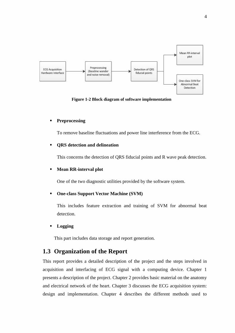
algorithm (one-class SVM) for abnormal beat detection. Figure 1-2 presents a block
diagram view of the software implementation.
Figure 1-1 Block diagram of hardware implementation
4
Preprocessing
To remove baseline fluctuations and power line interference from the ECG.
QRS detection and delineation
This concerns the detection of QRS fiducial points and R wave peak detection.
Mean RR-interval plot
One of the two diagnostic utilities provided by the software system.
One-class Support Vector Machine (SVM)
This includes feature extraction and training of SVM for abnormal beat
detection.
Logging
This part includes data storage and report generation.
1.3 Organization of the Report
This report provides a detailed description of the project and the steps involved in
acquisition and interfacing of ECG signal with a computing device. Chapter 1
presents a description of the project. Chapter 2 provides basic material on the anatomy
and electrical network of the heart. Chapter 3 discusses the ECG acquisition system:
design and implementation. Chapter 4 describes the different methods used to
Figure 1-2 Block diagram of software implementation

5
interface ECG acquisition hardware with a computation device. Chapter 5 discusses
preprocessing of the ECG for noise removal and an algorithm for QRS complex
detection. It also includes a discussion of R wave peak detection and the generation of
mean RR interval plot. Chapter 6 delineates a method for using one-class SVM for
abnormal beat detection using training data from one class. Chapter 7 presents the
conclusions and discusses future work which could build upon the work contained in
this thesis.

6
2 The Human Heart
This chapter describes the structure and functional working of the heart. A brief
overview of the electrical activity in the heart is presented. It also provides a brief
introduction to the electrocardiogram. Cardiac abnormalities are usually reflected in
the ECG and an understanding of the electrical network of the heart can therefore be
beneficial.
2.1 Electrical Conduction System of Heart Cardiac cells contract systematically and rhythmically. The contraction of heart is a
direct consequence of the contraction of all of the tiny cells of heart. These
contractions of the heart cells are triggered by electric impulses generated by the
Sinoatrial (SA) node within the heart as shown in Figure 2-1. The cells in the SA node
depolarize resulting in a pulse which travels throughout the heart and serves as a
stimulus for other cells of the heart. To understand the origin of these electrical
impulses, we should be familiar with the concept of action potentials in the heart.
2.1.1 Action Potentials in the Heart
We know that each cell is surrounded by a semi permeable membrane known as cell
membrane. The cell membrane allows ions to move in and out of the cell. Since ions
are charged particles, their movement establishes a potential gradient across the cell
membrane known as membrane potential. Due to this membrane potential every cell
Figure 2-1 Heart’s Conduction System [3]

7
in our body is slightly negative (at rest) inside than outside. The resting membrane
potential of a cell is approximately -0.1Volt [3].
Action potential is the tendency of cells to rapidly reverse their resting
membrane potential from negative value to slightly positive value which is usually
known as depolarization. The change in potential from this slightly positive value to
resting membrane potential is called repolarization. The cells which are capable of
reversing their resting membrane potentials are called excitable cells. Cardiac cells are
excitable cells. Action potentials occurring in the cardiac cells play a critical role in
systematic and rhythmic beating of the heart.
2.1.2 Initiation and Propagation Action Potentials in the Heart
The rhythm of the heart is initiated by the action potentials generated automatically by
the cells of sinoatrial (SA) node of the heart. The action potentials arising in the cells
of sinoatrial (SA) node propagate to and through atrioventricular (AV) node to Bundle
of His and Purkinje fibers. This propagation of action potentials through the heart
synchronizes the heart. As a result, all the cells contract at the same time which results
Figure 2-2 Action Potentials in heart [4]

8
in systematic and rhythmic beating of the heart. The initiation and transmission of
action potentials in the heart is shown in Figure 2-2.
2.2 Measurement of Electrical Activity in the Heart
The propagation of action potentials in the heart results in an electric pulse traveling
through the heart. The characteristics of this electric pulse can be measured by using
an electrocardiogram (ECG). The electrocardiogram is an indirect way of measuring
the electrical activity in the heart. A device for recording ECG was invented by
William Einthoven in 1901.
An electrocardiogram is obtained by measuring the potential difference between
different points on the body. A detailed analysis of the heart’s electrical activity can
be carried out by studying the ECG which also helps in the diagnosis of various
cardiac disorders.
2.3 ECG Systems
Electrodes placed on the skin, which are used to obtain an electrocardiogram, provide
a view of the heart’s electrical activity in the shape of a waveform. An ECG records
these waveforms from different perspectives called planes and leads.
A lead provides a view of the heart’s electrical activity between a positive and
a negative pole. The two poles define the lead’s axis. The term “axis” refers to the
direction of the current moving through the heart. The direction of the current affects
the direction of the ECG waveform. If the current is moving towards a positive pole,
it causes an upward deflection on the ECG and vice versa.
Plane refers to a cross-sectional view of electrical activity in the heart. For
example the frontal plane provides an anterior-to-posterior view of electrical activity.
2.3.1 The 12-Lead ECG System
The 12-lead ECG consists of 12 leads that are places on the limbs and chest. These 12
leads provide 12 different views of the heart’s electrical activity.
The six limb leads - I, II, III, augmented vector right (aVR), augmented vector
left (aVL), and augmented vector foot (aVF)- provide information about the heart’s

9
vertical plane. The augmented leads are unipolar while the other three limb leads are
bipolar.
The six chest, or precordial leads - V1, V2, V3, V4, V5, and V6 - provide
information about electrical activity in the heart’s horizontal plane. The precordial
leads are unipolar just like the augmented limb leads. These unipolar leads have
another indifferent electrode at the center of the heart.
2.3.1.1 Limb Leads
Figure 2-3 shows the placement of the limb leads where LL refers to the left leg. The
three bipolar limb leads form the basis of Einthoven’s Triangle. The augmented limb
leads are derived from the same three electrodes as in leads I, II, III. A brief
explanation follows:
Lead I is bipolar with positive electrode on the left arm and negative electrode
on the right arm.
Lead II is bipolar with positive electrode on the left leg and negative electrode
on the left arm.
Lead III is bipolar with positive electrode on the left leg and negative
electrode on the right arm.
Lead aVR has the positive electrode on the right arm. The negative electrode
is a combination of the left arm and leg electrodes.
Lead aVL has the positive electrode on the left arm and the negative electrode
is a combination of the right arm and left leg electrodes.
Lead aVF has the positive electrode on the left leg while the negative
electrode is a combination of the right arm and left leg electrodes.
Together these leads from the “hexaxial” reference system. The hexaxial reference
system is used to determine the heart’s electrical axis in the vertical plane. The term
electrical axis refers to the general direction of the heart’s depolarization wavefront
[3].

10
2.3.1.2 Precordial Leads
The precordial leads are placed in a sequence across the chest. They provide a view of
the heart’s horizontal plane. The six electrodes are considered positive and a negative
reference is calculated. Figure 2-4 shows the placement of the precordial leads.
Figure 2-3 Limb lead placement [3]
Figure 2-4 Precordial lead placement [3]

11
2.3.2 Three Electrode ECG System:
The system used for ECG acquisition in this project is similar to lead I of the limb
leads with an additional right leg drive. The right leg drive is used to remove
electromagnetic interference and provides a reference point for the ECG signal. Since
we are only using one of the leads, the ECG signal obtained will only provide
information about the heart’s electrical activity from perspective of lead I. The
acquisition system has been described in a later section.
2.4 ECG Waveform
This section describes a typical ECG waveform and its various components. Figure
2-5 shows a typical ECG waveform. The baseline voltage of the ECG is known as the
isoelectric line. A discussion of the components follows.
2.4.1 P Wave
The P wave is the first component of the ECG waveform and represents atrial
depolarization. The P wave is usually seen upright in lead I (which we are using). If
the deflection of the P wave is normal and the P wave precedes the QRS complex, this
means that the electrical activity originated in the SA node. A normal P wave is 0.06
to 0.12 seconds in duration [3].The relationship between P waves and QRS complexes
allows us to distinguish between various cardiac arrhythmias.
Figure 2-5 ECG waveform [3]

12
2.4.2 QRS Complex
The QRS complex represents the depolarization of the ventricles and follows the P
wave. The depolarization of the ventricles causes them to contract and pump blood
through the arteries. The QRS complex looks “spiked” since the Bundle of His and
Purkinje fibers coordinate the depolarization of the ventricles leading to an increase in
conduction velocity. A normal QRS complex is 0.06 to 0.10 seconds in duration [3].
The Q wave is generally represented by the first negative deflection after the P
wave, the R wave is represented by the first positive deflection after the Q or P wave,
and the S wave is represented by the first negative deflection after the R wave. The
QRS usually appears upright in lead I. Every QRS complex may not contain a Q
wave, an R wave, and an S wave. A missing QRS complex may indicate AV block
while deep and wide Q waves may represent myocardial infarction.
2.4.3 T Wave
The T wave represents the repolarization of the ventricles. The T wave is usually
upright in lead I. The period from the beginning of QRS complex to the apex of the T
wave is known as the absolute refractory period. The last half of the T wave is called
the relative refractory period. During the relative refractory period the cells are
vulnerable to extra stimuli and a bump in the T wave may indicate that a P wave is
hidden in it. Tall or peaked T waves might indicate myocardial injury while inverted
T waves may represent myocardial ischemia [3].
2.4.4 U Wave
The U wave is not always visible on the ECG. It represents the repolarization of the
Purkinje fibers. A prominent U wave may be due to hypercalcemia or hypokalemia,
among other causes.
2.4.5 PR Interval
The PR interval represents the movement of the atrial impulse through the AV node,
Bundle of His and the right and left bundle branches.
Short PR intervals may indicate the impulse did not originate at the SA node.
Prolonged PR intervals may represent a conduction delay through the AV node due to
conduction tissue disease, ischemia, heart block etc.

13
2.4.6 QT Interval
The QT interval measures ventricular depolarization and repolarization and is around
0.40 seconds in duration [3]. The length of the QT interval varies according to the
heart rate. The faster the heart rate the shorter the QT interval.
2.4.7 ST Segment
The ST segment represents the end of ventricular depolarization and the start of the
ventricular repolarization. The ST segment starts at the J point, the junction between
the QRS complex and the ST segment, and ends at the start of the T wave. The ST
segment is typically 0.08 to 0.12 seconds long [3]. A depressed ST segment may
indicate myocardial ischemia. ST segment elevation may indicate myocardial
infarction.

14
3 ECG Acquisition This chapter describes ECG acquisition: techniques to acquire an ECG and the
different parts of the acquisition circuit.
3.1 Basic Concept
ECG acquisition circuit can be divided into following parts as in Figure 3-1.
1) Electrodes
2) Instrumentation amplifier
3) Filtering to remove noise
3.1.1 Electrodes
An amplifier usually has high input impedance and ideally the input current is zero.
However a non-zero current flows from the bio potential electrode to input of the
amplifier. In human body current is carried out by ions. While in the wires connecting
the electrodes to the amplifier, the current is carried out by electrons. A transducer,
represented by ECG electrodes in the circuit, is used for the interface between the
body (ionic current) and the amplifier circuit (electronic current).
3.1.1.1 Electrode Groups
Ideally bio potential electrodes have two groups. In non-polarizable electrode current
flows freely across the electrode-electrolyte interface. These electrodes behave as
resistors as in Figure 3-2
Polarizable electrodes have no transfer of charge between electrode-electrolyte
interfaces. These electrodes behave as capacitors as shown in Figure 3-3 [4]. The
current that flows is displacement current. Practical electrodes have characteristics in-
between polarizable and non-polarizable electrodes as neither of the two can be
fabricated.
Figure 3-1 Block Diagram of ECG Acquisition Circuit

15
3.1.2 Electrode Types
There are three types of electrodes. A brief discussion of each follows.
Dry electrodes do not use gel to make conducting path between surface of skin
and electrode. Due to lack of electrolyte their characteristics resemble those of
polarizable electrodes.
Non-contact electrodes use remote sensing of bio potential. These are safe as
no current is drawn from the body. To extract bio potential signal from non-contact
electrode, the input impedance of the amplifier should be very high.
Wet electrodes use gel as electrolyte between skin and the electrode. Their
characteristics approach those of non-polarizable electrodes. The most commonly
used type is Ag/AgCl (silver-silver chloride) electrode. The gel is used to conduct
current between electrode and skin surface. In our project we used wet electrodes as
these electrodes are cheap and can be used with long connecting wires due to their
low impedance.
3.1.3 Amplifier
The basic purpose of a bio amplifier is to amplify an extremely weak signal. The
greatest challenge is to extract a weak bio potential signal (.5 mV-5 mV) [5]. For long
term power autonomy of circuit, power dissipation of amplifier has to be minimized.
Furthermore signal obtained by electrode is coupled with DC signal of up to 300mV
[5].
Figure 3-2 Polarizable Electrode Figure 3-3 Non Polarizable Electrode

16
3.1.3.1 Instrumentation Amplifier
The wires connected to the electrodes are directly connected to the instrumentation
amplifier. A highly sensitive instrumentation amplifier is used, as ECG signal is in
millivolts. The instrumentation amplifier should amplify ECG signal while
attenuating common mode signals. Common mode rejection ratio (CMRR) defines
the ability of the instrumentation amplifier to reject voltages common to both inputs.
Only the differential input is amplified. The most popular topology of the
instrumentation amplifier is the three op-amp topology shown in Figure 3-4 [6].
Operational amplifier OA1 and OA2 provide infinite input impedance while
amplifying differential input. The common mode gain Ac and differential gain Ad are
given by equation 3.1 and 3.2.
𝐴𝑑 = (
1
2+
𝑅2
𝑅1) (
𝑅4,𝑡𝑜𝑝
𝑅3,𝑡𝑜𝑝+
𝑅4,𝑡𝑜𝑝
𝑅3,𝑡𝑜𝑝(
𝑅4.𝑏𝑜𝑡𝑡𝑜𝑚
𝑅3.𝑏𝑜𝑡𝑡𝑜𝑚 + 𝑅4.𝑏𝑜𝑡𝑡𝑜𝑚)
+ 𝑅4.𝑏𝑜𝑡𝑡𝑜𝑚
𝑅3.𝑏𝑜𝑡𝑡𝑜𝑚 + 𝑅4.𝑏𝑜𝑡𝑡𝑜𝑚)
(3.1)
𝐴𝑐 = (1 +
𝑅4,𝑡𝑜𝑝
𝑅3,𝑡𝑜𝑝) (
𝑅4.𝑏𝑜𝑡𝑡𝑜𝑚
𝑅3.𝑏𝑜𝑡𝑡𝑜𝑚 + 𝑅4.𝑏𝑜𝑡𝑡𝑜𝑚) − (
𝑅4,𝑡𝑜𝑝
𝑅3,𝑡𝑜𝑝)
(3.2)
Figure 3-4 Three Operational Amplifier Differential Amplifier
Topology [6]

17
While using discrete component implementation of the instrumentation
amplifier, optimal performance in term of high common mode rejection ratio
(CMRR), stability, and differential gain are difficult to compute. In discrete
component implementation it is important to have accurately matched resistors. The
slightest error in resistor R3,top R3,bottom, and R4,top, R4,bottom results in unwanted
common mode amplification.
The three op-amp topology of instrumentation amplifier is available as an
integrated circuit. Integrated instrumentation amplifiers, such as AD620, vastly
outperform their discrete component implementation. AD620 draws maximum of
1.3mA supply current [7]. An op-amp such as LF353 draws 6.5mA per chip [8].
AD620 was chosen since it is cheap and is available in the market. The gain of
AD620 is controlled by a single external resistor. The gain is given by equation 3.3.
𝐺𝑎𝑖𝑛 = 1 +
49.9𝑘𝛺
𝑅𝐺
(3.3)
3.1.4 Filtering
To talk about filtration we must first be acquainted with the common sources of noise
that can degrade the ECG.
3.1.4.1 Noise
There are many sources of noise that affect the ECG such as electromagnetic
interference (EMI), noise due to muscle movement, radio interference etc. We have
only worked on removing EMI since it is a major source of noise.
Electromagnetic interference causes a lot of problem in acquiring ECG.
Electromagnetic interference is caused by the magnetic field produced by current
carrying conductors. When this magnetic field cuts the loop made by human body,
electrode lead and amplifier, it produces electromagnetic interference. The power
component of line frequency is very high and it overpowers the ECG signal since the
ECG signal is a low frequency signals (0-150 Hz) [4] and its power is small. Line
interference can be minimized by decreasing the length of wires connecting the
electrodes and the amplifier, implementing a filter, using a Faraday cage etc.

18
3.1.4.2 Low Pass Filter
The output of instrumentation amplifier is band limited by a low pass filter. A Low
pass filter is required because the output of instrumentation amplifier still has a large
component of line frequency. Simple RC passive low pass filter was used for filtering
purpose.
3.2 ECG Acquisition System
The ECG acquisition system that was used has three electrodes. Two electrodes are
used to acquire the ECG signal (Right arm and Left arm). The third electrode provides
a reference for the ECG signal. The system can be divided in the following parts as
shown in Figure 3-5.
1. Instrumentation amplifier
2. Right leg drive
3. Filtering
Figure 3-5 Block Diagram of three Lead ECG system
3.2.1 Instrumentation Amplifier
The instrumentation amplifier used to amplify differential input was AD620. The
connection scheme used has been shown in Figure 3-6 [5]. The right leg drive was
connected between two 22kΩ resistors. These resistors were used so that the gain of
AD620 can easily be changed by changing RG. These resistors also provide a
constant gain to the right leg drive. This configuration changes the gain formula of
AD620 and now it is given by equation 3.4.
𝐺𝑎𝑖𝑛 = 1 +
49.9𝑘𝛺
𝑅𝐺+
49.9𝑘𝛺
2 ∗ 22𝑘𝛺
(3.4)

19
The maximum gain of AD620 is 10,000 [7]. Ideally we would select the
maximum possible gain but the gain has to be selected keeping in mind that the output
does not saturate. Initially the gain was set to 10. After practical implementation the
gain was increased and the final gain of circuit was 100 i.e. RG=500Ω.
3.2.2 Right Leg Drive
The right leg drive injects an inverted version of the common mode signal into the
patient. This reduces the common mode signal at the inputs of AD620. The
operational amplifier used for this circuit was LF353. This circuit, shown in Figure 3-
7, act as a low pass filter with cut off frequency of 160 Hz (CLP=100nF, RLP=10kΩ).
3.2.3 Filtering
To band Limit the signal low pass and high pass filters were used. Low pass filter was
used to band limit the signal and to decrease the power component of 50 Hz
frequency. We used simple RC low pass filter with cut off frequency of 35 Hz as
shown in Figure 3-8. To provide high roll off, two low pass filters were connected in
series. High pass filter was used to remove DC offset present in ECG waveform. High
pass filter with cutoff frequency of 0.5 Hz was designed (R1 = 4.5 kΩ, R2 = 45kΩ,
R3 = 6.8 kΩ, C3 = 1 µF, C4 = 0.1 µF, C5 = 47 µF).
Figure 3-7 Leg Drive Figure 3-6 AD620 Circuit [5]
Figure 3-8 High pass and Low pass Filters
C31nF
R1
10k
R2
10k
R310k
C41nF
C5
1nF
20
4 Interfacing The last part of a data acquisition is concerned with making the analog ECG signal
available to a computer for further processing. From the various options available to
us for interfacing like serial bus, parallel bus, universal serial bus (USB), sound card
of PC, etc., we decided to choose,
1) Universal serial bus (USB)
2) Sound card of the PC
The original aim was to use USB but as an alternative, sound card of PC was also
used as a contingency plan. This was needed since the implementation of a USB
interface is a difficult task while interfacing with the sound card is relatively easier.
4.1 Interfacing using USB
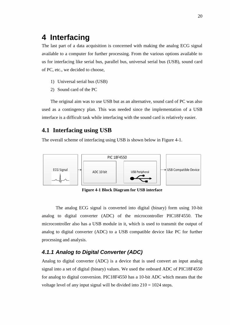
The overall scheme of interfacing using USB is shown below in Figure 4-1.
The analog ECG signal is converted into digital (binary) form using 10-bit
analog to digital converter (ADC) of the microcontroller PIC18F4550. The
microcontroller also has a USB module in it, which is used to transmit the output of
analog to digital converter (ADC) to a USB compatible device like PC for further
processing and analysis.
4.1.1 Analog to Digital Converter (ADC)
Analog to digital converter (ADC) is a device that is used convert an input analog
signal into a set of digital (binary) values. We used the onboard ADC of PIC18F4550
for analog to digital conversion. PIC18F4550 has a 10-bit ADC which means that the
voltage level of any input signal will be divided into 210 = 1024 steps.
Figure 4-1 Block Diagram for USB interface
21
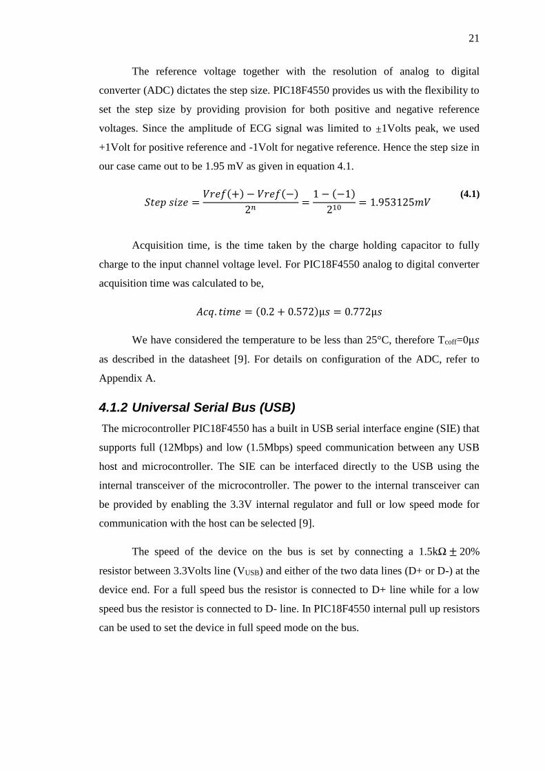
The reference voltage together with the resolution of analog to digital
converter (ADC) dictates the step size. PIC18F4550 provides us with the flexibility to
set the step size by providing provision for both positive and negative reference
voltages. Since the amplitude of ECG signal was limited to ±1Volts peak, we used
+1Volt for positive reference and -1Volt for negative reference. Hence the step size in
our case came out to be 1.95 mV as given in equation 4.1.
𝑆𝑡𝑒𝑝 𝑠𝑖𝑧𝑒 =
𝑉𝑟𝑒𝑓(+) − 𝑉𝑟𝑒𝑓(−)
2𝑛=
1 − (−1)
210= 1.953125𝑚𝑉
(4.1)
Acquisition time, is the time taken by the charge holding capacitor to fully
charge to the input channel voltage level. For PIC18F4550 analog to digital converter
acquisition time was calculated to be,
𝐴𝑐𝑞. 𝑡𝑖𝑚𝑒 = (0.2 + 0.572)µ𝑠 = 0.772µ𝑠
We have considered the temperature to be less than 25°C, therefore Tcoff=0µ𝑠
as described in the datasheet [9]. For details on configuration of the ADC, refer to
Appendix A.
4.1.2 Universal Serial Bus (USB)
The microcontroller PIC18F4550 has a built in USB serial interface engine (SIE) that
supports full (12Mbps) and low (1.5Mbps) speed communication between any USB
host and microcontroller. The SIE can be interfaced directly to the USB using the
internal transceiver of the microcontroller. The power to the internal transceiver can
be provided by enabling the 3.3V internal regulator and full or low speed mode for
communication with the host can be selected [9].
The speed of the device on the bus is set by connecting a 1.5kΩ ± 20%
resistor between 3.3Volts line (VUSB) and either of the two data lines (D+ or D-) at the
device end. For a full speed bus the resistor is connected to D+ line while for a low
speed bus the resistor is connected to D- line. In PIC18F4550 internal pull up resistors
can be used to set the device in full speed mode on the bus.

22
4.1.2.1 USB bus communication
There are four ways for the transmission of data on the universal serial bus [10].
1) Isochronous
2) Bulk
3) Interrupt
4) Control
We used interrupt mode of transfer for the transmission of ECG data to the PC
because it ensures data integrity timeliness of delivery.
4.1.2.2 Implementation of USB interface using PIC18F4550
From the data sheet of PIC18F4550 we can see that PORTC pins RC4 (pin23) and
RC5 (pin 24) are used for USB interface. RC4 is USB data D- pin and RC5 is USB
data D+ pin. Internal pull up resistors were used to configure the device in full speed
mode (12Mbps). The overall operation of the USB module of microcontroller is
controlled by three control registers and a total of twenty two registers to manage the
actual USB transactions. Instead of configuring these registers we used MikroC
library functions to implement USB transactions.
When a USB device is plugged into the bus, the process of enumeration
begins. In MikroC IDE we added a descriptor file which takes care of the process of
enumeration. This file was created using HID terminal of the MikroC IDE.
Configuration bits for the microcontroller were set by editing the project settings in
MikroC IDE.
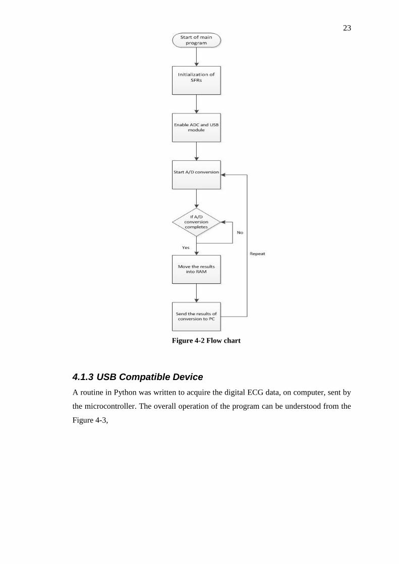
The working of the code written in C to convert the analog ECG signal to
digital form and transmit the output of analog to digital converter (ADC) to a PC
using USB can be understood from the flow chart shown in the Figure 4-2. The code
for conversion is present in Appendix C.
23
4.1.3 USB Compatible Device
A routine in Python was written to acquire the digital ECG data, on computer, sent by
the microcontroller. The overall operation of the program can be understood from the
Figure 4-3,
Figure 4-2 Flow chart

24
The method “Connect_USB” establishes the connection between the
microcontroller and the computer. After the connection is established, two processes
are initiated which run in parallel. Process1 (Acquire_Data) takes the ECG data,
output by the ADC of microcontroller, and puts it in the queue. Process2 takes the
data from the queue and can either save it to a file, stream it to another device or plot
it in real time.
The working of the methods “Acquire_Data”, “Save_File”, “Stream” and
“Real_Time_Plot” can be understood from the flow diagrams given in Figure 4-4,
Figure 4-3 Flow diagram for Main Method

25
The method Acquire_Data signals microcontroller to start sending data. The
data sent by microcontroller is received and converted into voltages. This data is then
sent to the queue. This process is executed in a cycle. A file is opened in writeable
mode. Data is read from the Queue and converted into strings. These strings are then
written to the file. The process is shown in Figure 4-5.
To stream data a socket must be created on both server and the client. The
server socket binds to its own IP address while the client socket connects to the server
IP address. A port common to both server and client is used for communication of
data. If the connection is established then communication process between server and
client starts. Flow diagram is shown in Figure 4-6.
Figure 4-5 Flow Diagram for the
Acquire_Data Method
Figure 4-4 Flow Diagram for the
Save_File Method

26
The Real_Time_Plot first creates an empty figure. The data is then read from
queue and put in a list. The list is then updated so that only new data is plotted. This
updated list is then plotted.The code for the complete routine and subroutines along
Figure 4-7 Flow Diagram for the
Real_Time_Plot Method
Figure 4-6 Flow Diagram for the Stream Method

27
with their documentation is given in Appendix D.
4.2 Interfacing using the Sound Card Input
As discussed in the beginning of the chapter, the sound card interface was developed
as a contingency plan. The microphone input to a PC, laptop or a smartphone is a
ready-made system for data-acquisition since it uses a built-in ADC to sample the
input signal. However, the microphone input suffers from at least two problems:
1) The input is capacitively coupled.
2) The sound card is usually designed to work for a band of frequencies between
20 Hz to 20 kHz.
The major component of an ECG signal lies between 0.5 – 50 Hz [11] . Figure 4-
8 shows the input frequency response of a PC sound card to a sine sweep (20 Hz -20
kHz). It can be seen that the roll off starts above 20 Hz in this particular case.
Most computing devices today have a sound card with a microphone input
with at least an 8 bit (usually higher) ADC. However, in order to make use of the
sound card for interfacing, the ECG band needs to be shifted to higher frequencies
due to the aforementioned problems. This can be readily achieved through Frequency
modulation of the ECG signal. Figure 4-9 shows a conceptual diagram of the
proposed system
Figure 4-8 Sound card frequency response

28
.
4.1.4 Frequency Modulation
Frequency modulation allows us to encode the low frequency ECG signal using a
high frequency carrier. The frequency of the carrier changes in relation to the
amplitude of the ECG signal. A frequency modulated wave can be described by
equation 4.2 [12].
𝜑𝐹𝑀(𝑡) = 𝐴 cos( 𝜔𝑐𝑡 + 𝑘𝑓 ∫ 𝑚(𝛼) 𝑑𝛼
𝑡
−∞
(4.2)
In equation 4.2, 𝜔𝑐 represents the carrier frequency while 𝑘𝑓 is known as the
sensitivity. Since FM represents the signal to be transmitted in the variation of the
frequency and not the amplitude of the carrier, we can read this frequency modulated
signal from the microphone input of the circuit using a software routine. We can also
read this signal at the microphone input using MATLAB.
4.1.5 Voltage to Frequency Converter
Voltage to frequency converters, basically VCOs, are available as integrated circuits
and can be used for linear frequency modulation. Another option is to implement a
voltage controlled oscillator through various circuit topologies using discrete
components. A V to F converter, however, allows the implementation of the
modulation scheme using a single IC.
4.1.6 V to F converter design
Texas instruments LM 331 voltage to frequency converter was selected for frequency
modulation since it meets the specifications and is available in the market. Since our
Figure 4-9 Block Diagram representation of proposed system

29
signal can take on both positive and negative voltages, we need a bipolar V to F
converter. LM 331 by itself does not allow us to cater to both positive and negative
voltage. To this end, the circuit of Figure 4-5 was designed to meet the specifications
in Table 4-1. LM331 provides a reference voltage of 1.90V at pin 2. In Figure 4-8 this
reference voltage has been used to allow bipolar voltage to frequency conversion.
4.1.6.1 Specifications
Table 4-1 Design Specifications
Input voltage range (Vp) +/- 1V
Sensitivity of VFC 2000 (Δf = 2 kHz for ΔVin = 1V )
Fo (center frequency) 4 kHz
Supply Voltage 9 V (battery)
4.1.6.2 Circuit Diagram:
4.1.6.3 Design:
The design equations are given below [13]. The circuit of Figure 4-10 was designed
using these equations to meet the specifications above.
𝐹 = 𝑉7 ∗
𝑅4
𝑁
(4.3)
Where V7 refers to the voltage at pin 7 and N is given by Eq. 4.4.
Figure 4-10 V to F converter circuit [13]

30
𝑁 = 2.09 ∗ 𝑅3 ∗ 𝑅2 ∗ 𝐶2 (4.4)
𝑅7 = (𝐹𝑝 − 𝐹𝑜) ∗ 1.9 ∗
𝑅1
𝐹𝑜 ∗ 𝑉𝑝
(4.5)
𝑅4 = 𝑁 ∗ 𝐹𝑜 ∗
2 ∗ 𝑅7 + 𝑅1
1.9 ∗ 𝑅1
(4.6)
In Eq. 4.5, Fp refers to the peak frequency of the VFC, Fo refers to center
frequency of VFC (Vin = 0V) and Vp is the peak input voltage. For our purposes we
chose Fo to be 4 kHz and Fp to be 6 kHz which gives a peak negative frequency, Fn,
of 2 kHz.
With these design parameters, we only need to change two resistors, R7 and
R4, to change our input voltage and output frequency range. The output available at
pin 3 is a stream of rectangular high-to-low pulses. For more details see [13].
Making use of Eqs.4.5 and 4.6, with the given design specifications, we
obtained the following values.
R4 calc = 86.7 k R4 used = 82 k
R7 calc = 95 k R7 used = 100k
Since the actual values used were different, a slightly different center frequency of 3.8
kHz was achieved.
4.1.6.4 Testing
The circuit was initially tested by applying DC voltages at pin 7 and observing the
output. Table 2 enumerates the results.
Table 4-2 DC testing of VFC circuit
Input (mV) Frequency (kHz) Input (mV) Frequency (kHz)
0 3.85 0 3.85
200 4.2 -200 3.4
400 4.6 -400 3
600 5 -600 2.6
800 5.4 -800 2.2
1000 5.8 -1000 1.8
31
The circuit was then tested by applying time varying voltages of various sorts and
observing the output at pin 3.
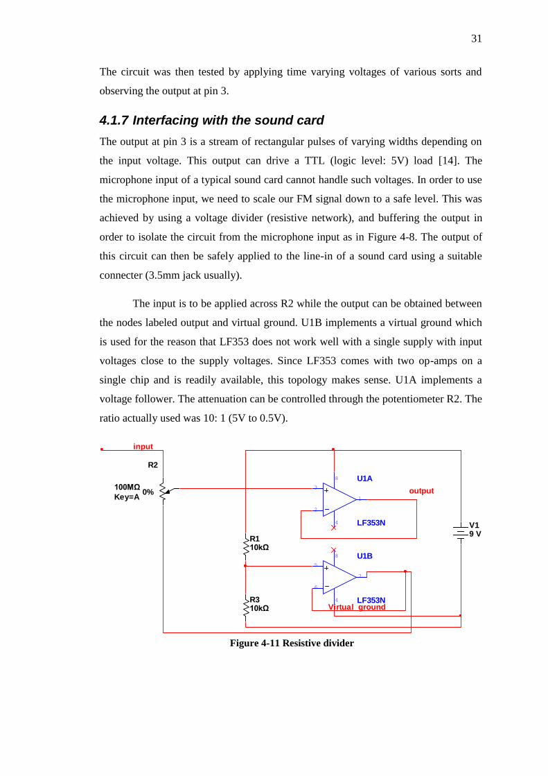
4.1.7 Interfacing with the sound card
The output at pin 3 is a stream of rectangular pulses of varying widths depending on
the input voltage. This output can drive a TTL (logic level: 5V) load [14]. The
microphone input of a typical sound card cannot handle such voltages. In order to use
the microphone input, we need to scale our FM signal down to a safe level. This was
achieved by using a voltage divider (resistive network), and buffering the output in
order to isolate the circuit from the microphone input as in Figure 4-8. The output of
this circuit can then be safely applied to the line-in of a sound card using a suitable
connecter (3.5mm jack usually).
The input is to be applied across R2 while the output can be obtained between
the nodes labeled output and virtual ground. U1B implements a virtual ground which
is used for the reason that LF353 does not work well with a single supply with input
voltages close to the supply voltages. Since LF353 comes with two op-amps on a
single chip and is readily available, this topology makes sense. U1A implements a
voltage follower. The attenuation can be controlled through the potentiometer R2. The
ratio actually used was 10: 1 (5V to 0.5V).
U1A
LF353N
3
2
4
8
1
R110kΩ
R2
100MΩ
Key=A0%
U1B
LF353N
5
6
4
8
7
V19 V
R310kΩ
output
Virtual_ground
input
Figure 4-11 Resistive divider

32
4.1.8 Demodulation
The FM signal can be read from the microphone input through MATLAB. MATLAB
also provides a built in function to demodulate FM signals. The MATLAB script
written for demodulation has been reproduced below.
%Set sampling frequency Fs=44000; %Create audiorecorder object y=audiorecorder(Fs,16,1,-1); %Read into the audiorecorder object from mic-in for 0.5 sec recordblocking(y,0.5); %Obtain samples from audiorecorder object z=getaudiodata(y); %Plot the signal read at the mic-in plot(z) %Demodulate FM with center freq. 3.8 kHz and sensitivity 2000 h=demod(z,3830,Fs,'fm',2000); %Open new figure window figure(2) %Plot demodulated signal in a separate window plot(h)
The demodulated output obtained using this code contained a considerable
amount of noise. However, before we could improve the modulating circuitry our
USB interface had been implemented and tested to work properly. Work on the sound
card interface was thus abandoned.

33
4.2 Acquisition and interfacing circuitry
Figure 4-12 shows the complete acquisition and interfacing circuit developed during
the course of this project.
pos
3 2
6
47
8
5
1
U1
AD
620
R5
22k
R6
22k
R7
500
32
1
84
U2
:A
LF
353R
8
10k
R9
1M
C6
.1U
F
1 2 3
J1
SIL
-10
0-0
3
5 6
7
8 4
U2
:B
LF
353
R10
10k
R11
10k
1 2
J2
SIL
-10
0-0
2
R12
4k6
R13
46k
C7
1u
F
C8
.1uF
1 2 3
J3
SIL
-10
0-0
3
RA
0/A
N0
2
RA
1/A
N1
3
RA
2/A
N2/V
RE
F-/
CV
RE
F4
RA
3/A
N3/V
RE
F+
5
RA
4/T
0C
KI/C
1O
UT
/RC
V6
RA
5/A
N4/S
S/L
VD
IN/C
2O
UT
7
RA
6/O
SC
2/C
LK
O14
OS
C1/C
LK
I13
RB
0/A
N12
/IN
T0
/FLT
0/S
DI/S
DA
33
RB
1/A
N10
/IN
T1
/SC
K/S
CL
34
RB
2/A
N8/IN
T2
/VM
O35
RB
3/A
N9/C
CP
2/V
PO
36
RB
4/A
N11
/KB
I0/C
SS
PP
37
RB
5/K
BI1
/PG
M38
RB
6/K
BI2
/PG
C39
RB
7/K
BI3
/PG
D40
RC
0/T
1O
SO
/T1
CK
I15
RC
1/T
1O
SI/C
CP
2/U
OE
16
RC
2/C
CP
1/P
1A
17
VU
SB
18
RC
4/D
-/V
M23
RC
5/D
+/V
P24
RC
6/T
X/C
K25
RC
7/R
X/D
T/S
DO
26
RD
0/S
PP
019
RD
1/S
PP
120
RD
2/S
PP
221
RD
3/S
PP
322
RD
4/S
PP
427
RD
5/S
PP
5/P
1B
28
RD
6/S
PP
6/P
1C
29
RD
7/S
PP
7/P
1D
30
RE
0/A
N5/C
K1S
PP
8
RE
1/A
N6/C
K2S
PP
9
RE
2/A
N7/O
ES
PP
10
RE
3/M
CLR
/VP
P1
U3
PIC
18
F4
550
WD
T_
PE
RIO
D=
18m
C9
10
0nF
C10
10
0nF
VC
C1
D+
3
D-
2
GN
D4
J4
AU
-Y1
00
5-R
X1
CR
YS
TA
L
C11
22
pF
C12
22
pF
C13
47
0uF
R19
4K
7123456
J5
CO
NN
-H6
3 2
6
7 4
1
5
U4
741
R15
6.8
K
R16
6.8
K
R17
6.8
K
R18
6.8
K
RV
1
10K
C14
10
uF
R14
16K
RV
2
10K
RV
3
10K
R0
10k
R01
10k
C1
1n
F
C2
1n
F
R02
10k
R03
10k
Figure 4-12 Complete circuit

34
5 Artifact Removal and QRS Complex
Detection This chapter presents an overview of artifacts which usually distort an ECG signal
and the techniques that were implemented for the removal of these artifacts along
with an algorithm for QRS complex detection. These artifacts lower the accuracy of a
diagnosis based on such an ECG and therefore their removal is imperative to ensure a
reliable diagnosis. Section-1 deals with the artifacts normally present in an ECG and
the techniques that were used for their removal. Section-2 presents an algorithm for
QRS detection. Section discusses a method to detect R wave peak. The python code
for these analyses can be found in Appendix E.
5.1 Artifact Removal
This section presents the artifacts that distort the ECG and the techniques used for
their removal. For QRS complex detection, the ECG has to be preprocessed in order
to remove these artifacts.
5.1.1 ECG Artifacts
The ECG signal is usually corrupted by the following types of artifacts [15] :
1. Power line interference: This presents itself as a 50/60 Hz noise in the ECG.
The noise frequency drifts with the change in the power line frequency.
2. Baseline Drift: Baseline drift can usually be attributed to relative motion
between the electrode contact surface and the skin and presents itself as a 0.15
– 0.3 Hz signal [16].
3. Quantization noise and aliasing introduced due to digitization of the ECG.
Figure 5-1 shows an ECG signal acquired using our own ECG acquisition system.
Baseline drift and noise distorting the ECG is clearly visible. In order to use this ECG
for diagnosis we need to remove these artifacts to get a cleaner signal.
5.1.2 Artifact Removal Techniques
This section discusses the techniques implemented for baseline wander and power
line interference removal.

35
5.1.2.1 Baseline wandering
Baseline wandering can be thought of as a shift in the DC value of the signal and can
usually be attributed to relative motion between the electrode contact surface and the
skin. Baseline wander has a frequency range 0.05 – 1 Hz [16]. Baseline wander can
cause problems in QRS detection and its removal is therefore necessary.
Baseline wander removal techniques can be broadly classified in two
categories: polynomial based and filtering based techniques. While polynomial based
techniques are more robust, filtering based techniques are easier to implement. A
simple high pass filter of cutoff frequency around 0.5 Hz can be used for baseline
removal. The high pass filter should have linear phase filter in order to avoid
distortion of the ECG.
Linear phase filtering can be achieved by using a finite impulse response (FIR)
filter. However FIR filters designed for this purpose are of very high order (700 Hz –
2000 Hz) and cannot be implemented on small datasets due to the delay introduced by
FIR filtering. To deal with this problem, infinite impulse response (IIR) forward-
backward filtering can be used since an IIR filter with a similar frequency response to
an FIR filter usually has a smaller order. Furthermore forward-backward filtering with
an IIR filter is equivalent to forward filtering with a filter of squared magnitude and
zero phase response [17].
Figure 5-1 ECG with baseline wander and power line interference

36
5.1.2.2 Power line Interference removal
Power line interference generally presents itself as a 50 or 60 Hz signal added on to
the ECG signal. A common method to remove power line interference is to use a
digital notch filter to remove frequency components around the power line frequency.
However, this does not take into account the drift in the power line frequency and
again requires a filter of a very high order due to the small transition band.
Since our main goal is the detection of QRS start and end points we do not
need to preserve the entire ECG spectrum. An ECG signal with frequency
components in the range 0.5 -45 Hz is adequate for QRS detection [18].Therefore we
can use a low pass digital filter to limit the band of frequency range of the ECG signal
below 50 Hz. While this will distort the ECG, the resulting signal would work for our
purposes.
5.1.3 Implementation and Results
Since baseline wander removal can be achieved using a 0.5 Hz high pass filter while
power line interference can be reduced through a 45 Hz low pass filter, a Chebyshev
band pass filter of 0.5 – 45 Hz was used for forward backward filtering of the ECG.
Figure 5-2 shows the frequency response of the Chebyshev filter designed for this
purpose. The order of this bandpass filter is 7 and through forward backward filtering
the computational complexity which would have been a problem for say a 500 order
FIR filter has been reduced.
Figure 5-2 Chebyshev bandpass filter frequency response

37
Figure 5-3 compares a raw and bandpass filtered ECG.
5.2 QRS detection
As detailed before, the QRS complex represents the depolarization of the ventricles.
The detection of the QRS complex is of prime importance in ECG analysis since a
fair number of subsequent processing steps are based on this.
5.2.1 The Length Transform for QRS detection
We implemented a length transform based algorithm for QRS detection. The
algorithm is similar to the popular Pan-Tompkins algorithm. Figure 5-4 presents a
block diagram view of the steps involved in QRS complex detection using the length
transform algorithm.
Figure 5-3 Raw and forward backward bandpass filtered ECG
Figure 5-4 Length transform algorithm for QRS detection

38
The algorithm relies on the fact that if we view the ECG signal as being made
up of a string, the QRS complexes would consume most of the length of the string i.e.
the curve length corresponding to the QRS complex is longer than that of other parts
of the ECG. More formally, the curve length corresponding to the QRS complex can
be written as in Eq. 4.1. Here Tx represents the sampling interval and yi represents the
amplitude of the i-th ECG sample while n is the length of the QRS complex in terms
of the samples [19].
𝐿 = ∑ 𝑙𝑖
𝑛
𝑖=1
∑ √𝑇𝑥2 + (𝑦𝑖 − 𝑦𝑖−1)2
𝑛
𝑖=1
Eq.
4.1
Eq. 4.1 reduces to Eq. 4.2 if we approximate the length of each hypotenuse (𝑙𝑖)of the
triangle with the height. Figure 5-5 illustrates this concept.
𝐿 = ∑ 𝐷𝑦𝑛𝑖=1 Eq.
4.2
Since 𝐷𝑦 can be negative we will use 𝐷𝑦2 for the purpose of analysis. Note that
𝐷𝑦 is simply the first order difference of the signal. Since the curve length for QRS
complex is generally greater than for any other part of the ECG, this approximation
would allow us to identify the QRS complex simply by taking the first order
difference of the signal.
5.2.2 Implementation and Results
The implementation of the length transform algorithm for QRS detection follows in
the order specified in Figure 5-4.
𝑦𝑖−1
𝐷𝑦
𝑇𝑥
𝑦𝑖
Figure 5-5 Illustration of the approximation for length transform

39
5.2.2.1 Band Pass filtering
The frequency content of the QRS complex lies between 10-25 Hz [18].A band pass
filter designed for this frequency range would remove the low frequency noise
attributed to movement or baseline shifts and the high frequency noise, including
power line interference, from the ECG. An FIR filter was used for this purpose.
Figure 5-6 presents the ECG signal filtered by a band pass (10-25 Hz) filter.
5.2.2.2 Differentiation
As discussed before, the curve length of the ECG signal can be approximated by first
order difference of the signal. Figure 5-7 compares the band pass filtered and the
difference signal. It can be seen that the first order difference has large values for the
samples corresponding to the QRS complexes.
Figure 5-6 The preprocessed ECG filtered by a 10-25 Hz band pass filter
Figure 5-7 First order difference of the band pass filtered signal

40
5.2.2.3 Squaring
The differenced signal is then squared. Figure 5-8 shows the results.
5.2.2.4 Thresholding
In order to detect the QRS complex, a threshold is defined by averaging the difference
squared signal over a window of duration four seconds. A noise factor multiplier is
provided to account for the amount of noise in the signal. The samples of the
Figure 5-8 Difference squared
Figure 5-9 Threshold values

41
difference squared signal greater than the threshold value are marked as potential
QRS complexes. Figure 5-8 shows the threshold plotted with the difference squared
signal.
Figure 5-10 illustrates the potential QRS complex region obtained through this
process. The figure shows the difference squared values obtained for a single QRS
complex. In order to detect the actual QRS complex post processing is required to
remove the errors (regions erroneously marked as QRS complex) and to detect QRS
start and end points since the QRS can be divided into multiple regions as in Figure 5-
10.
5.2.2.5 Morphological post processing
To remove errors and detect QRS start and end points we use morphological opening
and closing. Morphological opening is used to remove small spikes in the identified
potential QRS complex regions which usually appear due to noise while
morphological closing is used to join together potential QRS complex regions if they
are close enough. To perform morphological opening, a ones array corresponding to
0.12*fs duration (normal QRS length) was used as the structuring element. For
morphological closing a ones array corresponding to 0.04*fs duration (minimum QRS
length) was used as the structuring element. Figure 5-11 illustrates the result of
Figure 5-10 Thresholding and potential QRS complex region

42
morphological opening and closing. It can be seen that an isolated spike marked as a
potential QRS complex region has been removed (morphological opening) while the
spikes which were adjacent have been marked as QRS complex regions
(morphological closing).
5.2.2.6 Detection of QRS fiducial points
Since the regions comprising the QRS complexes are now well defined, a simple
difference operation can now be used to find the QRS start and end or fiducial points.
Figure 5-12 depicts the results.
Figure 5-11 Results of morphological opening and closing
Figure 5-12 QRS fiducial points

43
5.2.2.7 Results
This algorithm is good at detection of the QRS complex but the fiducial points
identified by this algorithm need to be further refined to increase the accuracy.
5.3 R wave
This section presents a simple method to detect the R peak. Furthermore we present a
plot of the running average of the RR-intervals.
5.3.1 R peak detection
Since the QRS start and end points have been marked, we use a crude method to
approximate the peak of R wave by taking the average of the QRS start and points.
This method is not very accurate and is contingent upon the detection of the QRS
complex. The R wave peaks approximated by this method have been marked in
Figure 5-13.
5.3.2 RR interval
Since we know the approximate R wave peak location, we can now plot RR-intervals.
Figure 5-14 presents the running average of the three consecutive RR-intervals. It can
be seen that the RR-interval length varies.
Figure 5-13 R peak approximation

44
Figure 5-14 Mean RR interval plot
45
6 Support Vector Machine for Abnormal
Beat Detection This chapter details the method used for abnormal cardiac beat detection. A one-class
Support Vector Machine (SVM) trained on QRS complex samples was used as a
classifier since negative examples were not available. The Python code for one-class
SVM has been reproduced in Appendix E.
6.1 Support Vector Machines
The detection of abnormal cardiac beats is a classification problem. That is, by
analyzing each cardiac beat in an ECG record we have to determine whether the beat
is normal or abnormal. Since ECG morphologies vary across individuals, therefore to
classify a particular individual’s cardiac beats as abnormal we need a Machine
Learning algorithm that can be trained using that particular individual’s ECG. A
classifier trained using a large number of “normal” beats from different individuals
might not work for another individual. A support vector machine is a classifier which
given labeled training data, produces an optimal function which can then be used to
categorize new examples. We use a one-class SVM for abnormal cardiac beat
detection.
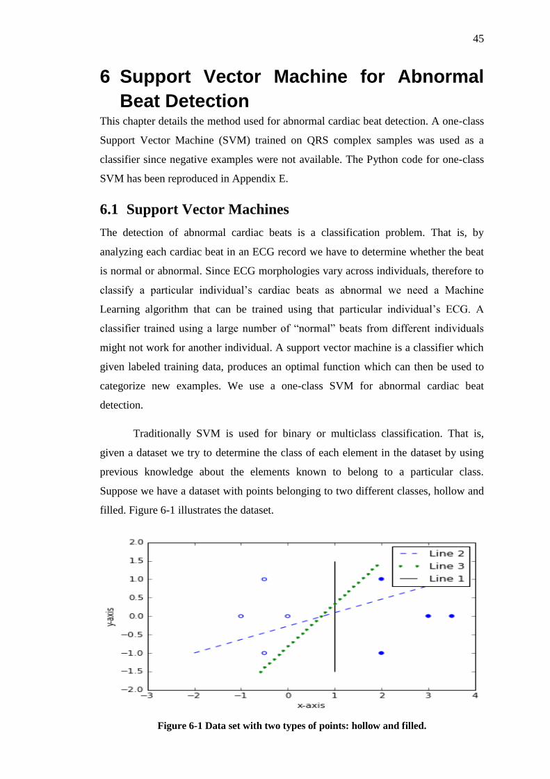
Traditionally SVM is used for binary or multiclass classification. That is,
given a dataset we try to determine the class of each element in the dataset by using
previous knowledge about the elements known to belong to a particular class.
Suppose we have a dataset with points belonging to two different classes, hollow and
filled. Figure 6-1 illustrates the dataset.
Figure 6-1 Data set with two types of points: hollow and filled.

46
We can separate the two classes by drawing a line since the data is linearly separable.
In Figure 6-1 line 1 and line 3 separate the data while line 2 fails to do so. We can use
line 1 and line3 as classifiers. The optimal classifier however would maximize the
perpendicular distance from data points belonging to the two classes since it would
reduce the chance of error if a new data point were now to be introduced and
classified. The points that lie closest to the separating line in this example are called
support vectors. Figure 6-2 marks the support vectors for line 1 and line 3.
Support Vector Machines are linear classifiers that produce the optimal
separating boundary, line 1 in this case, given a set of labeled training data. Once the
separating boundary has been learned, new data points (testing data) can then be
classified.
Formally for a two-class support vector machine, consider the data set Ω =
(𝑥1, 𝑦1), … (𝑥𝑛, 𝑦𝑛) where 𝑥𝑖 ∈ 𝑅𝑑 and 𝑦𝑖 ∈ −1, 1 and 𝑦𝑖 indicates the class of
input vector 𝑥𝑖 [20]. The SVM uses a linear discriminant function to differentiate
Figure 6-2 Support Vectors

47
between input vectors ‘x’ belonging to different classes. This linear discriminant
function is given in Eq. 6.1.
𝑓(𝑥) = 𝑠𝑔𝑛(𝑤𝑇𝑥 + 𝑏) ( 6.1)
An SVM training algorithm finds ‘w’ and ‘b’ in such a way so as to maximize
the margin, as in Figure 6-2, while classifying all the marked training points correctly.
That is we need to maximize the margin ‘ρ’, as in Eq. 6.2, while fulfilling the
conditions in Eqs. 6.3 and 6.4 [21].
max ρ =
2
‖𝑤‖
(6.2)
𝑤𝑇𝑥𝑖 + 𝑏 ≤ −1 ∀ 𝑖 𝑠. 𝑡. 𝑦𝑖 = −1 (6.3)
𝑤𝑇𝑥𝑖 + 𝑏 ≥ 1 ∀ 𝑖 𝑠. 𝑡. 𝑦𝑖 = 1 (6.4)
In order to classify data points which cannot be separated by a linear classifier
in their original space𝐼, the data points are projected to a feature space 𝐹 through a
non-linear function 𝛷 where they can be separated by a hyperplane. The hyperplane
projected back to original space 𝐼 has the form of a non-linear curve. To avoid over
fitting in the presence of noisy data and to provide a solution to the non-linear
problem, we use a slack variable 𝜉𝑖 ≤ 0 to allow some data points to lie inside the
margin ‘ρ’. This is known as soft margin SVM. In general we do not project the input
vector to the feature space and use a ‘kernel function’ which has the same effect [21].
This is known as the ‘kernel trick’. Eqs. 6.2 – 6.4 change as in Eqs. 6.5 - 6.6 due to
introduction of the slack variable.
min 1
2 𝑤𝑇𝑤 + 𝐶 ∑ 𝜉𝑖
𝑁
𝑖=1
(6.5)
such that
𝑦𝑖(𝑤𝑇𝑥𝑖 + 𝑏) ≥ 1 − 𝜉𝑖
(6.6)
The parameter C determines the penalty due to margin violation.

48
6.2 One-class SVM
The previous section was geared towards a general treatment of SVM where we had
to differentiate between two or more classes. However, since we only have normal
ECG recordings, we need to use one-class SVM. One-class classifiers use training
examples from only one class to generate a conception of the data which can then be
used to determine whether a new sample point belongs to that class or not.
Formally given training examples( 𝑧𝑖 , 𝑖 = 1 … 𝑁 ), one-class SVM generates
a decision function 𝑓(𝑧) = 𝑤𝑇𝛷(𝑧) + 𝑏 such that for data in the target class, 𝑓(𝑧) ≥
0 while 𝑓(𝑧) < 0 for outliers. ‘w’ is chosen such that the hyperplane 𝑓(𝑧) lies at a
maximum perpendicular distance from the origin [22].
Analogous to the parameter C in traditional SVM, one-class SVM uses a
parameter ′𝜐′ which sets an upper bound on the fraction of outliers in training set and
a lower bound on the number of training examples used as support vector.
The approach discussed below uses randomly selected beats from an ECG
record to train a one-class SVM algorithm. This particular method has been shown to
reach Sensitivity (Se)/Specificity (Sp) of 87.6%/95.8% [23].
6.3 Implementation
This section discusses the implementation of one-class SVM used for abnormal beat
detection.
Figure 6-3 Feature extraction

49
6.3.1 Feature Extraction
In order to apply one-class SVM we need to extract features from the ECG. We
assume that all the beats in the sample are normal. A 0.6 second interval of samples,
centered on the R wave, was extracted from randomly selected R waves in the ECG
recording. One third of all such samples were used for training while the rest were
used for testing. Figure 6-3 presents a sample of the ECG records used for training.
6.3.2 Training and Testing
One-class SVM was implemented using scikit-learn, a Python machine learning
library. The aforementioned randomly selected ECG records were used as training
data while the rest of the samples in the recording were used for testing. The one-class
SVM algorithm returns +1 for input vectors classified as belonging to the target class
while it returns -1 for outliers. Figure 6-4 presents the results obtained for one ECG
recording with a polynomial kernel. Generally with a soft-margin SVM,
misclassifications are unavoidable.
6.3.3 Evaluation
For proper evaluation of one-class SVM, we would need a set of known outliers to
test our particular implementation of one-class SVM. Since the ECG data isn’t
annotated that sort of evaluation isn’t possible. In the ideal scenario, we would have
an ECG record with abnormal and normal beats annotated by a cardiac expert. In that
Figure 6-4 Training and testing errors

50
case we can calculate sensitivity and specificity to provide a metric for the accuracy
of the algorithm.

51
7 Conclusions and Future Work
This work was aimed at the design of an ECG acquisition and analysis system. The
main focus of this work has been the implementation of a flexible interface for our
acquisition hardware and the detection of QRS complexes for abnormal beat
detection. In this chapter we present our conclusions about different techniques
implemented in this work along with the issues which can be resolved in another
undertaking of a similar nature.
The ECG signal obtained from our acquisition hardware is contaminated with a
number of artifacts of which power line interference has proven to be intractable.
While analog and digital filtering of the ECG, as discussed above helps, a more robust
acquisition circuitry with better common mode rejection ratio and a greater focus on
analog filtering can increase the reliability of the acquisition circuitry. Furthermore,
the acquisition circuitry currently only provides the option for single lead (lead I)
ECG acquisition.
A microcontroller was used to digitize the acquired ECG and to develop a USB
interface for our acquisition hardware. We wrote an application to communicate with
our acquisition module from a Personal Computer or Laptop. The application allows
the user to acquire ECG, view it by generating a plot, saving it to a file and to stream
the acquired signal to a remote server. This application has been tested to work on
Linux based systems. The development of an application to do the same using an
android or other cell phone would greatly enhance the portability of the acquisition
module.
Forward backward band pass (0.5 -45 Hz) filtering of the acquired signal was
implemented in order to reduce the computational complexity introduced by a high
order FIR filter with similar characteristics. The filter successfully removes baseline
variations and reduces the noise added through power line interference.
The identification of QRS complexes is a fundamental component of an automated
ECG analysis system. The length transform algorithm was used for detection of QRS
fiducial points and R wave peak detection. The QRS complex comprises a majority of
the curve length of the ECG and the length transform algorithm approximates the

52
curve length through a simple difference operation of the acquired sample values. The
algorithm is reliable but the QRS start and end points can be detected with greater
accuracy using other algorithms. The detection of the R wave peak in our system
hinges on the correction detection of QRS complex fiducial points since we
approximate the R wave peak as the midpoint of the QRS start and end.
The system implements two main diagnostic utilities. First, it allows the user to view
the running average of the RR intervals. Secondly, we have implemented a one-class
SVM to detect abnormal cardiac beats. Both of these utilities would benefit from a
cleaner ECG record. Furthermore, the one-class SVM would function better with a
better feature extraction mechanism and a larger ECG record which would provide
more data for training. The one-class SVM can be supplemented or replaced by other
classification techniques. If annotated ECG training data were available, a binary
SVM could be used.
The integrated system can be used as a portable device for long term remote
monitoring of cardiac patients. If the android interface were available, the acquisition
circuitry along with an android phone could be used to stream an ECG record to a
remote server for analysis which can then alert a medical expert if needed. The system
can thus be used as portable monitoring system
The analysis algorithms can be coupled with a database of ECG records of different
patients for automatic analysis of the ECG. This would reduce the burden on a cardiac
expert since the expert could then only review the ECG records flagged by the
analysis system.

53
Appendix A
Parameter Setting of ADC
The 10-bit analog to digital converter (ADC) module of PIC18F4550 consists of five
registers.
1) A/D Result High Register (ADRESH)
2) A/D Result Low Register (ADRESL)
3) A/D Control Register 0 (ADCON0)
4) A/D Control Register 1 (ADCON1)
5) A/D Control Register 2 (ADCON2)
The result of an A/D conversion is loaded into ADRESH: ADRESL register pair. The
remaining three registers are used to control the operation of analog to digital
converter (ADC) module.
The configuration of the three control registers of ADC module for converting analog
ECG signal to digital (binary) form are described below with details,
A.1 A/D Control Register 0 (ADCON0)
The various bits in the register are shown below in Figure A-1.
The analog to digital converter (ADC) module of PIC18F4550 has thirteen input
channels. Among the available channels we selected channel 0(AN0). Therefore the
values for analog channel select bits become,
CHS3:CHS0
0000 = Channel 0 (AN0)
Initially the module remains disabled so,
Figure A-1 ADCON0 Register

54
ADON = 0
The value of GO/ DONE doesn’t matters if ADON=0.
GO/ DONE = 0
A.2 A/D Control Register 1 (ADCON1)
The various bits in the register are shown below in Figure A-2.
Since the amplitude of analog ECG signal varies from -1Volts to +1Volts, we have to
use external reference voltages for analog to digital converter module. The values for
voltage reference configuration bits are,
VCFG1 = 1
VCFG2 = 1
Since we required only one channel (AN0) to be used for analog input, the values for
A/D port configuration bits are,
PCFG3:PCFG0 = 0000
A.3 A/D Control Register 2 (ADCON2)
The various bits in the register are shown below Figure A-3.
The result of analog to digital conversion was right justified; therefore the value of
A/D result format select bit was selected to be,
ADFM = 1
Figure A-2 ADCON1 register
Figure A-3 ADCON2 register

55
The minimum acquisition time for PIC18F4550 was 0.772µs. The microcontroller
was operating at 48MHz. Thus the values for A/D acquisition time select bits came
out to be,
ACQT2:ACQT0
111 = 20TAD
The A/D conversion clock select bits were selected to be,
ADCS2:ADCS0
100 = Fosc /4

56
Appendix B
UNIVERSAL SERIAL BUS (USB)
The universal serial bus (USB) is a high speed serial interface that is used to
transmit digital data to a PC. The bus can also power up the devices connected to it. A
USB interface is implemented using four wires as discussed below,
Table B-1 USB wires specification
Pin Name Wire color Description
1 VBUS Red +5 Volts
2 D- White Data -
3 D+ Green Data +
4 GND Black Ground
PIC18F4550 has a USB peripheral which supports full speed (12Mbps) and low speed
(1.5Mbps) communication with any USB host and microcontroller.
B.1 Configuration Bits
Configuration bits of a microcontroller allow the user to customize certain
aspects of the device to the needs of the application. When the device powers up, the
state of these bits determines the modes that the device uses. The settings made for
configuration bits during the development of the project are given below,
External oscillator was selected
HS,PLL was enabled
The clock source for USB was set from the output of PLL
The default values of other configuration bits were used
Pre-scaler value was set to 5
Post-scaler value was set to 2
B.2 Description of MikroC USB Library Functions
Following MikroC USB library functions were used in the project.

57
1 Hid_Enable (&readbuffer, &writebuffer)
This function enables the USB communication and requires two arguments: Read
buffer address is the location in microcontroller RAM where data sent by host is
stored. Write buffer address is the location in microcontroller RAM where data sent
by microcontroller is stored. This function must be called before calling any other
functions of the USB library.
2 Hid_Read ( )
This function receives the data from USB bus and stores in the read buffer. It
returns the number of characters received.
3 Hid_Write (&writebuffer, length)
This function sends the data from write buffer to the USB bus. The name of the
buffer and the length of the data to be sent must be specified as arguments to the
function. The function does not return any data.
4 Hid_Disable ( )
This function disables the USB data transfer. It has no arguments and returns no
data.
5 Usb_Interrupt_Proc ( )
This function is used for servicing various USB bus events. The function requires
no parameters. It must be ensured before using this function that USB interrupts are
enabled.

58
Appendix C
Code for USB interface implementation
/*----------------------------------- Description:----------------------------------------
The code accomplishes the following tasks,
1. Converts analog ECG signal to a set of 10-bit digital values.
2. Transmit the digital ECG signal to a PC using USB.
* Test configuration:
MCU(Microcontroller): PIC18F4550
http://ww1.microchip.com/downloads/en/DeviceDoc/39632D.pdf
Oscillator: HS 20.000 MHz (USB osc. is raised with PLL to 48.000MHz)
-------------------------------------------End of Description-----------------------------*/
//Buffers should be in USB RAM , please consult datasheet for details
unsigned char readbuff [64] absolute 0x500;
unsigned char writebuff [64] absolute 0x540;
//Variables are used to measure the USB data transfer time and minimize the //variation in
sampling time
int value;
int new_value;
//Variable used to count the number of conversions
int i;
//-------------------------------------USB Interrupt Service Routine---------------------
void interrupt()
USB_Interrupt_Proc();
//------------------------------------End of Interrupt Service Routine----------------------
--
//------------------------------------Start of Main Function--------------------------------
----
void main()
INTCON = 0x80; //Enable Interrupts
ADCON0 = 0x00; //Initially disabling the analog to digital converter
// and selecting channel AN0
ADCON1 = 0x00; //Configuring all the ports as analog and setting
//internal voltage ref.
ADCON2 = 0xBC; //Making the required settings as described in the section
//for ADCON2
T0CON=0x08; //Required Settings for Timer Zero

59
TMR0IE_bit=0; // Timer Zero Interrupt Disabled
TMR0L=0x00; //Load Timer Zero with 0
TMR0H=0x00;
i = 0;
label: HID_Enable(&readbuff , &writebuff); //Enable HID Communicatio
while (!HID_Read()); //Wait Unless a read operation is successful
ADCON0 = 0x01; // Enable ADC
TMR0ON_bit =1 ; //Start Timer Zero
while (!HID_Read()) //Continue Loop unless a read operation is
//successful
GO_DONE_bit = 1; //Start ADC conversion
while (GO_DONE_bit == 1); //Wait unless the conversion is complete
writebuff [i] = ADRESL; //Write the results of conversion to USB RAM
writebuff [i+1] = ADRESH;
i=i+2;
if (i==64) //Check that 32 conversions are complete or not
TMR0L=0x00; //Load Timer0 with Zero
TMR0H=0x00;
while (!HID_Write(&writebuff , 64)); //Send the results of Conversion to PC
value = TMR0H<<8+TMR0L; //Read the time for USB
//transfer
new_value = 65536-24000-value; //new_time = 2.2ms - time
TMR0L = new_value; //Load Timer0 with new time
TMR0H = new_value>>8;
TMR0IF_bit = 0; //Set Interrupt Flag to Zero
while(!TMR0IF_bit); //Wait until timer0 interrupt occurs
i = 0; //Set i=0
continue; //Start new conversion by going to the
//top of loop
delay_us(2200); //Sampling Time
goto label;
//-------------------------------End of Main Function-------------------------------------

60
Appendix D
Python code for USB compatible Device
'''
The code is written for Python3 and operates correctly when run from the terminal shell on
Linux Ubuntu version 14.04.
'''
# : For one line comments
#''':For multiple line comments
# importing the required modules
import multiprocessing
import usb.core
import usb.util
import matplotlib.pyplot as plt
import socket
import tty,select,sys,termios
import binascii
import struct
import sys
import random
'''
Connect_USB method connects the microcontroller to the PC. The Vendor and Product for the
microcontroller are 0x0001 and 0x1234
respectively. The method searches for the device and then detaches the kernel driver, which
was connected to the device upon connection. The configuration for the device is then set and
addresses for the ENDPOINT IN and ENDPOINT OUT are obtained.
'''
def Connect_USB():
global dev,reattach,endpoint #Make the variables global
dev = usb.core.find(idVendor = 0x0001,idProduct = 0x1234)
#Find the device with the given Vendor and Product ID
reattach = False
if dev.is_kernel_driver_active(0):
#Checks whether the kernel driver is active or not. If kernel driver
reattach = True
#is active then detach the kernel driver.
dev.detach_kernel_driver(0)
dev.set_configuration()
#Set the configuration for the device.
cfg = dev.get_active_configuration()
intf = cfg[(0,0)]

61
endpoint = (dev[0][(0,0)][0])
ep = usb.util.find_descriptor(
intf, custom_match = \
lambda e:\
usb.util.endpoint_direction(e.bEndpointAddress)== usb.util.ENDPOINT_IN)
#Adresses for ENDPOINT IN and ENDPOINT OUT
'''
The method Acquire_Data has a queue(Que) as an argument. This method gets the data from the
usb and puts it in the queue after converting the ten bit ADC results into a corresponding
integer.
'''
def Acquire_Data(Que):
dev.write(0x01,[1])
#Write '1' to the microcontroller so that process of data sending starts
temp_64 = [] #Empty list to save data
while (True):
data = dev.read(endpoint.bEndpointAddress,endpoint.wMaxPacketSize,5000)
#Read data sent by the microcontroller with a timeout=5ms
length = len(data) #Finding Length of data
for i in range(int((length-2)/2)):
temp = [data[2*i],data[2*i+1]]
num = int.from_bytes(temp,'little',signed = False)
#Converting data bytes to integer
temp_64.append(num)
temp_data = list(temp_64) #Copying List to a new list
Que.put(temp_data) #Writing data to the queue.
del temp_64[0:] #Deleting items from the list
'''
The method Save_File has also queue as an argument. The data in queue is read and written to
the file.
'''
def Save_File(Que):
step = 5/1024 #Step used to convert data integers into voltages
file = open('ecg.txt','w') #Open a file 'ecg.txt' in write mode
while (True):
read = list(Que.get()) #Read data from the queue and convert it into list.
for i in range(len(read)):
file.write(str(read[i]*step)+'\n')
#Writing to file after making strings of the voltages and appending a new line #chracters
'''
The method Stream has also a queue as an argument(Que). A socket is created and connected to
the server ip 192.168.233.107. the communication will happen through the port '10000'. A
structure object packer is created. The argument shows that this structure will operate on a

62
data that is list with 32 items and items are integers. Packer object is used to pack(convert
to binary) the data in values which was read from queue. The binary data is then converted to
hex format and sent to the server.
'''
def Stream(Que):
sock = socket.socket(socket.AF_INET, socket.SOCK_STREAM)
#Create a TCP/IP socket
server_address = ('192.168.233.107', 10000)
sock.connect(server_address) #Connect to socket
values = Que.get() #Read values from the Queue
packer = struct.Struct('I '*32) #Creating Packer object
packed_data = packer.pack(*values) #Converting Values to binary
try:
print ('sending "%s"' % binascii.hexlify(packed_data), values)
#Converting binary data to hex format
sock.sendall(packed_data) #Send data through socket
finally:
print ('closing socket')
sock.close() #Closing socket
'''
The method Real_Time_Plot has also a queue as an argument. The function creates a figure and
plots a line corresponding to y = 0 for 1000 points. Limits for the y-axis of the plot are
then set to the range '-10' to '10'. The data is then read from the queue and put in y. The
data is then updated and plotted
'''
def Real_Time_Plot(Que):
fig = plt.figure() #Create an empty figure
ax = fig.add_subplot(111) #Add a subplot to the figure
y = [0]*1000
li, = ax.plot(y) #Create a plot object later used to plot updated data
plt.grid(True) #Turn grid on
fig.canvas.draw()
plt.show(block = False) #Show Plot
plt.ylim((-10,10)) #Set y-limits
while (True):
read = qu.get() #Read data from queue
del y[0:len(read)]
y = y+a
li.set_ydata(y) #Plot updated data
fig.canvas.draw()
del read[0:]

63
'''
The function isData monitors the terminal for input. If their is an input on the terminat the
function returns 1 otherwise 0.
'''
def isData():
return select.select([sys.stdin], [], [], 0) == ([sys.stdin], [], [])
'''
The method main gets the setting of the terminal before performing any other task. The method
Connect_USB is called afterwards and if the connection is established 'USB_Connected' is
printed. A multiprocessing queue is then formed which is used to share data between two
processes. Two processes are then created and started which run in paralell. The first process
calls the fuction Acquire_Data while the second process can call any one of the fuctions
'Save_File' , 'Real_Time_Plot' or 'Stream'. The main then monitors the terminal for input. If
'ESc' key is pressed the main terminates the child processes and also stops the
microcontroller by writing '1' to the microcontroller.In the end, the device is reattached to
the kernel driver.
'''
if __name__ == "__main__":
old_settings = termios.tcgetattr(sys.stdin) #Get the settings of terminal
Connect_USB() #Calls the Connect_USB method
print ('USB_Connected')
que = multiprocessing.Queue()
#Creates a Queue to share data between processes
p1 = multiprocessing.Process(target = Acquire_Data, args = (que,))
#Define processes. Target specifies the function to be run as a seperate process
p2 = multiprocessing.Process(target = Stream, args = (que,))
p1.start() #Start both processes
p2.start()
try:
tty.setcbreak(sys.stdin.fileno())
#Monitors the terminal for input. If 'Esc' key is pressed the finally block executes
while (True):
if isData():
c = sys.stdin.read(1)
if (c == '\x1b'):
break
finally:
termios.tcsetattr(sys.stdin, termios.TCSADRAIN, old_settings)
#Reassign the old settings to terminal
p1.terminate() #Close process 1 and 2
p1.join()
p2.terminate()
p2.join()

64
usb.util.dispose_resources(dev)
dev.attach_kernel_driver(0) #Reattach Kernel driver
print ('USB_Disconnected')
#---------------------------------Server code for Host--------------------------------
import binascii
import socket
import struct
import sys
# Create a TCP/IP socket
sock = socket.socket(socket.AF_INET, socket.SOCK_STREAM)
server_address = ('192.168.233.107', 10000)
sock.bind(server_address)
sock.listen(1) #Server listens to a single client
unpacker = struct.Struct('I '*32) #A structure used to unpack the data sent by client
while True:
print ('\nwaiting for a connection')
connection, client_address = sock.accept()
try:
data = connection.recv(unpacker.size)
print ('received "%s"' % binascii.hexlify(data)) #Convert binary to hex format
unpacked_data = unpacker.unpack(data)
print ('unpacked:', unpacked_data)
finally:
connection.close() #Close Connection

65
Appendix E
Python Code for ECG Analysis
from scipy import signal, ndimage
from numpy import array,diff, append,int8,where,mean, int32, floor, std
import numpy as np
from numpy import ones as np_ones
from matplotlib import pyplot as plt
from random import randint
from sklearn import svm
#-------------------------------------------------Read ECG function---------------------------
def read_ecg():
file_name = input("Please enter path and name of file ") #Recorded ECG file
if file_name == '':
file = open ('D:\\University\\7th Semester\\FYP\\python\\hasan1_ecg.txt','r')
else:
file = open (file_name, 'r')
ecg_sig = [] #For reading data from file
for i in file:
ecg_sig.append(int( file.readline() ) )
file.close()
return ecg_sig
#------------------------------------------------ Block Processing function (mean) -----------
def funm(data,length):
'''funm(data,length) takes mean of each window of length "length" in data.
Data should be a list
inputs:
data - a list containing data points
length - window length for mean calculation
output:
z - a list of length "len(data)" with elements replaced by mean of elements
falling in each window of length "length"
example:
>>> z = funm([1,2,3,4,5] , 2)
>>> print(z)
[1.5, 1.5, 3.5, 3.5, 5.0]
'''
z = []
number = floor(len(data) / length)
zeros = int32((len(data) - number*length ))
for i in range(int32(number)):
block = data [i*length:(i+1)*length]

66
ones = length*[mean(block)]
z.extend(ones)
lst_mean = mean(data[-zeros:])
ones = zeros*[lst_mean]
z.extend(ones)
return z
#----------------------- Block Processing function (standard deviation) ---------------------
def funs(data,length):
'''funs(data,length) takes mean of each window of length "length" in data.
Data should be a list
inputs:
data - a list containing data points
length - window length for mean calculation
output:
z - a list of length "len(data)" with elements replaced by standard deviation of
elements
falling in each window of length "length"
example:
>>> z = funs([1,2,3,4,5] , 2)
>>> print(z)
[1.5, 1.5, 3.5, 3.5, 5.0]
'''
z = []
number = floor(len(data) / length)
zeros = int32((len(data) - number*length ))
for i in range(int32(number)):
block = data [i*length:(i+1)*length]
ones = length*[std(block)]
z.extend(ones)
lst_std = std(data[-zeros:])
ones = zeros*[lst_std]
z.extend(ones)
return z
#--------------------------------QRS detection function --------------------------------------
---
def QRS_LT (samp, ecg_sig,noise_fac = 0.5):
''' QRS_LT(samp,ecg_sig,noise_fac) implements the length transform method
for QRS detection based on a simple derivative approach.
inputs:
samp: sampling frequency
ecg_sig: a list (not np.array) containing ecg data points

67
noise_fac: a factor which can be used to suppress the effects of noise
on QRS detection. For high noise, choose a noise factor closer to 1.
The default value is zero.
outputs:
index_on: list containing sample numbers indicating start of a QRS
index_off: list containing sample numbers indicating end of a QRS
Note that the two lists are populated such that we first count a QRS starting
point and then the ending point. This means that if ecg_sig contains a QRS
ending point without a starting point, it will be neglected.
'''
MF = 2.0
qrs_size = 0.12*samp
min_qrs_size = 0.04*samp
nyq = samp/2
#----------------------------- Bandpass filtering --------------------------------------------
coeff = signal.firwin2 (101, [0, 8/nyq, 10/nyq, 25/nyq, 27/nyq, 35/nyq, nyq/nyq],
[0,0.7,1,1,0.7,0,0], window = 'blackman')
initial = 100
delay = (initial // 2) #Remove delay introduced by
FIR filter
ecg_sig.extend(delay*[0]) #Append zeros equal to delay at the end
ecg_sig = signal.lfilter (coeff, 1, ecg_sig) #Filter
ecg_sig = ecg_sig[delay:] #Remove delay so that filtered and original
#data line up
#----------------------------- Differentiation and squaring ---------------------------------
ecg_sig = diff (ecg_sig)
# h = array([-2, -1, 1, 2])/8
ecg_sig = append(ecg_sig,[0])
ecg_sig = [i**2 for i in ecg_sig]
#------------------------------ Thresholding ------------------------------------------------
T_win = 4*samp
threshold = funm(ecg_sig,T_win)
#Call block processing function(mean) with window length T_win
noise_fac = noise_fac*max(threshold)
threshold = noise_fac + MF*array(threshold)
decision = (ecg_sig > threshold )
decision.dtype = int8
#--------------------------------------Morphological closing and opening --------------------
struct_close = np_ones(qrs_size)
#structure for morphological closing
decision = ndimage.morphology.binary_closing(decision,struct_close)
decision.dtype = int8
#function returns bool

68
struct_open = np_ones(min_qrs_size) #structure for morphological opening
decision = ndimage.morphology.binary_opening(decision,struct_open)
decision.dtype = int8
#function returns bool
decision1 = append(diff(decision), [0])
#after difference: 1 denotes start of QRS, -1 end of QRS (plot it)
#----------------------------------------Find indices ---------------------------------------
index_on = where(decision1 == 1) #returns tuple
index_on = index_on [0]
#first element of tuple contains the array of our interest
index_off = where(decision1 == -1)
index_off = index_off [0]
if (len(index_on) > 0 and len(index_off) > 0): #Non-empty
if (index_off[1] < index_on[1]):
index_off [1] = []
#ECG starting index < ECG closing index
if (len(index_off) == 0 or (index_on[-1] > index_off[-1])):
index_on [-1] =[]
#Again only sets of QRS onset and offest are being included
else:
index_on = []
index_off = []
return index_on, index_off
#-----------------------------------------Band pass filter------------------------------------
def bandpass_filter(samp, ecg_sig):
'''
bandpass filters the signal using chebyshev filter of order using forward
backward filtering
input:
samp: sampling frequency in Hz
ecg_sig : Signal to be filtered
output:
response: forward backward filtered ecg_sig
b = np.array([ 0.06876288, -0.42392463, 1.19560393, -2.12170399, 2.69859612,
-2.50278218, 1.48077995, 0. , -1.48077995, 2.50278218,
-2.69859612, 2.12170399, -1.19560393, 0.42392463, -0.06876288])
a = np.array ([ 1.00000000e+00, -8.49604161e+00, 3.35577780e+01,
-8.22283201e+01, 1.40439389e+02, -1.77470173e+02,
1.71326048e+02, -1.28356988e+02, 7.49712127e+01,
-3.39410935e+01, 1.16939037e+01, -2.95566529e+00,
5.02936968e-01, -4.13786796e-02, -1.60836561e-03])
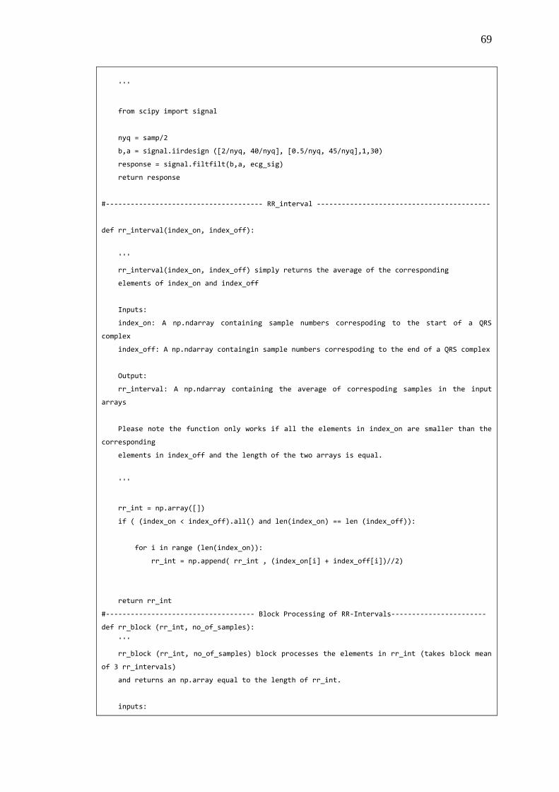
69
'''
from scipy import signal
nyq = samp/2
b,a = signal.iirdesign ([2/nyq, 40/nyq], [0.5/nyq, 45/nyq],1,30)
response = signal.filtfilt(b,a, ecg_sig)
return response
#-------------------------------------- RR_interval ------------------------------------------
def rr_interval(index_on, index_off):
'''
rr_interval(index_on, index_off) simply returns the average of the corresponding
elements of index_on and index_off
Inputs:
index_on: A np.ndarray containing sample numbers correspoding to the start of a QRS
complex
index_off: A np.ndarray containgin sample numbers correspoding to the end of a QRS complex
Output:
rr_interval: A np.ndarray containing the average of correspoding samples in the input
arrays
Please note the function only works if all the elements in index_on are smaller than the
corresponding
elements in index_off and the length of the two arrays is equal.
'''
rr_int = np.array([])
if ( (index_on < index_off).all() and len(index_on) == len (index_off)):
for i in range (len(index_on)):
rr_int = np.append( rr_int , (index_on[i] + index_off[i])//2)
return rr_int
#------------------------------------ Block Processing of RR-Intervals-----------------------
def rr_block (rr_int, no_of_samples):
'''
rr_block (rr_int, no_of_samples) block processes the elements in rr_int (takes block mean
of 3 rr_intervals)
and returns an np.array equal to the length of rr_int.
inputs:

70
rr_int: Input list/np.array containing the sample point of an R in an ECG signal.
no_of_samples: Total number of samples of the ECG signal for which the RR_intervals
are to be calculated.
output:
An np.array 'c' which contains the average of three consecutive RR intervals
generated from rr_int.
'''
interval_length = diff(rr_int)
#Calculate rr_interval length
c = np.array([])
c = np.append(c , interval_length [0] *(np.ones(rr_int [0])))
#Array which holds average of each block of 3 RR - intervals
number = len(interval_length) // 3
zeros = len(interval_length) - number*3
for i in range (0, number*3, 3):
mean_value = (interval_length [i] + interval_length [i+1] + interval_length [i+2])/3
#Take mean
time_average_gen = mean_value*np.ones((rr_int[i+3] - rr_int[i]))
c = np.append (c, time_average_gen)
mean_value = mean(interval_length[-zeros:])
c = np.append(c, mean_value*(np.ones((no_of_samples - rr_int[number*3]))))
return c
#-----------------------------------------------Running mean--------------------------------
def moving_average(rr_int, total_samples, length = 3):
'''
mvoing_average() calculates the moving average of samples
in rr_int and returns an array c containing the running
average of the rr_intervals which can be directly plotted
'''
interval_length = diff(rr_int) #Calculate rr_interval length
weights = np.repeat(1.0, length)/length
mov_average = np.convolve(interval_length,weights,'valid')
#Moving average of RR intervals
boundary = np.array([mean(interval_length[-2:]), interval_length[-1]])
#Handle conditions at the boundary of the interval_length array
mov_average = np.append(mov_average,boundary)
c = np.array([])
c = np.append(c , interval_length [0] *(np.ones(rr_int [0])))
for i in range(0,len(mov_average)):
c = np.append(c,mov_average[i]*np.ones(rr_int[i+1]-rr_int[i]))
c = np.append(c, mov_average[-1] * np.ones(total_samples - rr_int[-1]))
return c

71
#-------------------------Extract samples for ONE CLASS SVM---------
def extract_samples(ecg_sig, samp, rr_int):
'''extract_samples(ecg_sig,samp,rr_int) extracts 0.6 seconds intervals around
each R wave and returns an array (numpy) of arrays which contains intervals
corresponding to each R wave.
output:
qrs: extracted qrs complex samples
sample_numbers: Start and end point of extracted QRS complexes
'''
intervals = []
qrs_sample_numbers = []
for i in range(0, len(rr_int)):
if i == 0:
if (rr_int [i] - int(samp*0.3)) >= 0:
intervals.append(ecg_sig[int(rr_int [i]) - int(samp*0.3) : int(rr_int [i]) +
int(samp*0.3)])
qrs_sample_numbers.append([int(rr_int [i]) - int(samp*0.3) , int(rr_int [i]) +
int(samp*0.3)])
elif i == len(rr_int)-1:
if( rr_int [i] + 0.3*samp) < len(ecg_sig):
intervals.append( ecg_sig [int(rr_int[i]) - int(samp*0.3): int(rr_int[i]) +
int(samp*0.3)])
qrs_sample_numbers.append([int(rr_int [i]) - int(samp*0.3) , int(rr_int [i]) +
int(samp*0.3)])
else:
intervals.append( ecg_sig [int(rr_int[i]) - int(samp*0.3): int(rr_int[i]) +
int(samp*0.3)])
qrs_sample_numbers.append([int(rr_int [i]) - int(samp*0.3) , int(rr_int [i]) +
int(samp*0.3)])
return intervals, qrs_sample_numbers
#----------------------------------ONE CLASS SVM---------------------------
def outlier_detection(qrs, rr_int):
'''
outlier_detection (qrs, rr_int) trains a one-class SVM with 1/3
of the samples in qrs for training and the rest for testing.
index_test contains indexes of "qrs" used for training
'''
length = int(len(qrs)/3) + 2
index_train = []
index_test = []
for i in range (length):
random_number = randint(0,len(qrs))
if (random_number not in index_train):
index_train.append(randint(0, len(qrs)-1))

72
index_train.sort()
X_train = []
X_test = []
for i in range(len(qrs)):
if (i in index_train):
X_train.append(qrs[i])
else:
X_test.append(qrs[i])
index_test.append(i)
classifier = svm.OneClassSVM(nu = 0.01, kernel = 'poly', gamma = 1, degree = 2)
classifier.fit(X_train)
pred_train = classifier.predict(X_train)
pred_test = classifier.predict(X_test)
error_train = where (np.array(pred_train) == -1) #Find indexes with -1
error_test = where (np.array(pred_test) == -1) #Find indexes with -1
errors_train = []
errors_test = []
train_error = []
#Sample number of QRS complexes which used for training and returned errors
test_error = []
#Sample number of QRS complexes which used for testing and returned errors
if (len(error_train[0]) != 0):
for h in range(error_train[0][-1]+1): #returns tuple
if (h in error_train[0]):
errors_train.append(index_train[h])
errors_train.sort()
for h in errors_train:
current = rr_int[h]
train_error.append(current)
if (len(error_test[0]) != 0):
for z in range(error_test[0][-1]+1):
if (z in error_test[0]):
errors_test.append(index_test[z])
errors_test.sort()
for b in errors_test:
current = rr_int[b]
test_error.append(current)
return train_error, test_error
#--------------------------------------------------------------------------------------------
samp = 500
ecg_sig = read_ecg()
x = list(ecg_sig)

73
ecg_sig = bandpass_filter (samp, list(map(lambda x :x,ecg_sig )) )
ecg_sig = ecg_sig.tolist()
ecg_sig1 = list(ecg_sig)
index_on, index_off = QRS_LT (samp,ecg_sig1)
rr_int = rr_interval (index_on, index_off)
mean_interval = (moving_average (rr_int, len(x)))/samp
time = (np.arange (0, len(ecg_sig))/samp).tolist()
plt.figure()
plt.subplot(211)
plt.vlines (rr_int, 0, 10, color = 'red', linestyles = 'solid', label = 'R wave')
plt.vlines (index_on,0,10, color ='blue', linestyles = 'dotted', label = 'QRS onset')
plt.vlines (index_off,0,10, color = 'green', linestyles = 'dashed', label = 'QRS offest')
plt.plot(ecg_sig, 'r--', label = 'ECG')
plt.xlabel ('Sample Number')
plt.ylabel ('Amplitude')
plt.title('QRS and RR interval annotated')
plt.legend()
plt.subplot(212)
plt.plot (time, mean_interval, 'r--', label = 'Mean RR interval' )
plt.ylabel('time(s)')
plt.xlabel('time(s)')
plt.title('Running mean of RR-interval')
plt.legend()
plt.tight_layout()
plt.show()
qrs, sample_numbers = extract_samples (ecg_sig, samp, rr_int)
train_error, test_error = outlier_detection(qrs, rr_int)

74
References
[1] A. Alwan, "Global status report on noncommunicable diseases," World Health
Organization, 2010.
[2] M. Hussain, N. Khan, M. Uddin and M. M. A. Nozha, "Chest Pain, Coronary
Artery Disease and Risk Factors:A Global Snapshot," Journal of the Dow
University of Health Sciences Karachi, vol. 8, no. 2, pp. 80-86, 29 September
2013.
[3] T. Diehl, ECG Interpretation made Incredibly Easy!, Pennsylvania: Lippincott
Williams & Wilkins, 2011.
[4] R. Yazicioglu, C. V. Hoof and R. Puers, Biopotential Readout Circuits for
Portable Acquisition Systems, Springer, 2009.
[5] Enrique, "ECG Front-End Design is Simplified with MicroConverter®," Analog
Dialogue, vol. 37, no. 4, pp. 10 - 14, 2003.
[6] A. Sedra and K. Smith, Microelectronic Circuits, 6th Edition, Oxford University
Press, 2009.
[7] A. Devices, "AD 620: Low drift, Low power Instrumentation Amplifier,"
[Online]. Available: http://www.analog.com/en/specialty-
amplifiers/instrumentation-amplifiers/ad620/products/product.html. [Accessed
1 January 2015].
[8] T. Instruments, "LF353," [Online]. Available: http://www.ti.com/product/lf353.
[Accessed 1 January 2015].
[9] Microchip, "PIC18F4550," [Online]. Available:
http://www.microchip.com/wwwproducts/Devices.aspx?dDocName=en010300.
[Accessed 1 January 2015].

75
[10] Compaq, HP, Intel, Lucent, Microsoft, NEC Philips, "Universal Serial Bus," 27
April 2000. [Online]. Available:
sdphca.ucsd.edu/Lab_Equip_Manuals/usb_20.pdf. [Accessed 1 January 2015].
[11] A. Bhat, V. Kumar and and S. Kumar, "Design of ECG Data Acquisition
System," International Journal of Advanced Research in Computer Science and
Software Engineering, vol. 3, pp. 676-680, April, 2013.
[12] B. Lathi, Modern Digital and Analog Communication Systems, 3rd Edition,
New York: Oxford University Press, 1998.
[13] "Sound Card Bipolar Voltage to Frequency," Interstellar Research, 2007.
[Online]. Available: http://www.daqarta.com/dw_kkvv.htm. [Accessed 1
January 2015].
[14] "LM231A/LM231/LM331A/LM331 Precision Voltage-to-Frequency
Converters," Texas Instruments, March 2013. [Online]. Available:
http://www.ti.com/lit/ds/symlink/lm331.pdf . [Accessed 1 January 2015].
[15] A. M. a. M. J. S. Kasar, "Performance of Digital filters for noise removal from
ECG signals in Time domain," International Journal Of Innovative Research In
Electrical, Electronics, Instrumentation And Control Engineering, vol. 2, no. 4,
pp. 1352-1355, 2014.
[16] V. Romero, "ECG baseline wander removal and noise suppression analysis in
an embedded platform," Universidad Complutense de Madrid, [Online].
Available:
URL:http://eprints.ucm.es/9886/1/ECG_baseline_wander_removal_and_noise_
suppression_in_an_embedded_platform.pdf. [Accessed 1 May 2015].
[17] J. Smith, "Introduction to Digital Filters with Audio Applications," Center for
Computer Research in Music and Acoustics (CCRMA),Stanford University,
2007. [Online]. Available: URL: http://ccrma.stanford.edu/~jos/filters/.
[Accessed 1 May 2015].
[18] V. Afonso, "ECG QRS Detection," in W.J. Tompkins, eds. Biomedical Digital

76
Signal Processing, New Jersey, Prentice Hall, pp. 236-264.
[19] G. M. D. J. W. Zong, "A Robust Open-source algorithm to Detect Onset and
Duration of QRS Complexes," in Computers in Cardiology, 2003.
[20] R. Vlasveld, "Introduction to One-Class Support Vector machines," 12 July
2013. [Online]. Available:
http://rvlasveld.github.io/blog/2013/07/12/introduction-to-one-class-support-
vector-machines/. [Accessed 1 May 2015].
[21] E. Alpaydin, Introduction to Machine Learning, London, England: The MIT
Press, 2010.
[22] K. C. S. F. e. a. P. Li, "An Abnormal ECG Beat Detection Approach for Long-
Term Monitoring of Heart Patients Based on Hybrid Kernel Machine
Ensemble," in Multiple Classifier Systems, Springer, 2005, pp. 346-355.
[23] F. A. Afsar, "A new novelty detector for finding abnormal beats in ECG
recordings," in International conference on Integrative Biology summit, Las
Vegas, 2013.


![Robust Inter-beat Interval Estimation in Cardiac …...Robust Inter-beat Interval Estimation in Cardiac Vibration Signals 5 2.1. Pre-Processing Let x raw[n] denote the raw digital](https://img.pdfslide.us/doc/110x75/5fb8e00055832c7a296b2ea6/robust-inter-beat-interval-estimation-in-cardiac-robust-inter-beat-interval.jpg)