Ablative Thermal Response Analysis Using the Finite Element Method

John A. Dec* NASA Langley Research Center, Hampton, Virginia, 23681

Robert D. Braun† Georgia Institute of Technology, Atlanta, Georgia, 30332-0150

A review of the classic techniques used to solve ablative thermal response problems is presented. The advantages and disadvantages of both the finite element and finite difference methods are described. As a first step in developing a three dimensional finite element based ablative thermal response capability, a one dimensional computer tool has been developed. The finite element method is used to discretize the governing differential equations and Galerkin’s method of weighted residuals is used to derive the element equations. A code to code comparison between the current 1-D tool and the 1-D Fully Implicit Ablation and Thermal Response Program (FIAT) has been performed.

Nomenclature A = area, m2 a = radiative heating nose radius constant b = radiative heating density constant Bi = pre-exponential factor for the ith resin component

cB′ = non-dimensional charring rate

gB′ = non-dimensional pyrolysis gas rate at the surface C = radiative heating constant based on planetary atmosphere C = Capacitance matrix CH = Stanton number for heat transfer cp = specific heat, J/kg-K Eai = activation energy for the ith resin component, Btu/lb-mole f(v) = radiative heating tabulated function of velocity Hr = recovery enthalpy, J/kg Hw = wall enthalpy, J/kg href = reference enthalpy at 298K, J/kg h∞ = free stream enthalpy, J/kg i = node index, resin component index (A,B,C) j = species index k = thermal conductivity, W/m-K Kc = Conductivity Matrix L = element length, m N = interpolation function n = time index P∞ = free stream pressure, N/m2 Pstag = stagnation pressure, N/m2

radq = stagnation point radiative heat flux, W/m2

*AIAA Member, Aerospace Engineer, Structural and Thermal Systems Branch, MS 431 †AIAA Fellow, David and Andrew Lewis Associate Professor of Space Technology, Guggenheim School of Aerospace Engineering

https://ntrs.nasa.gov/search.jsp?R=20090007598 2018-06-25T21:30:59+00:00Z

convq = stagnation point convective heat flux, W/m2

condq = conductive heat flux, W/m2

cwQ = cold wall heat flux, W/m2 rn = nose radius, m R = universal gas constant, Btu/lb-mole-°R R = load vector s& = recession rate, m/s T = temperature, °C Tw = wall temperature, °C t = time, sec ue = boundary layer edge velocity, m/s V = velocity, m/s x = distance measured from the original surface of the ablating material, m x = distance measured from the moving surface of the ablating material, m α = solar absorptivity ε = emissivity

of j

HΔ = enthalpy of formation of jth species, J/kg

δt = time step, sec Γ = resin volume fraction ρe = boundary layer edge gas density, kg/m3 ρ∞ = free stream density, kg/m3 ρ = solid material density, kg/m3 ρoi = original density of the ith resin component, lb/ft3 ρri = residual density of the ith resin component, lb/ft3 ρi = current density of the ith resin component, lb/ft3 σ = Stephan-Boltzman constant, W/m2-K4 ψi = density exponent factor

I. Introduction

HERE are two main types of thermal protection systems (TPS) in use today, reusable and ablative. Use of reusable TPS, like the space shuttle tiles or a metallic heat sink, is generally limited to low heat flux entry

trajectories1,2. Ablative TPS on the other hand can withstand large heat fluxes and heat loads and are generally used for vehicles which have a high entry velocity. In addition to high entry velocity, ablative TPS are also well suited where the target planet has a high atmospheric density such as Jupiter3. Ablative materials have been in use since the 1950’s where they were primarily used in the design and construction of ballistic missile nose cones. The success ablators demonstrated in re-entry applications made them attractive for use in rocket nozzle applications4. In general, the analysis of an ablative material’s thermal response requires the solution of a differential energy transport equation5. In one dimension, and neglecting pyrolysis gas flow, the form of this differential equation is given by equation (1) along with an associated decomposition or charring relation given by (2).

0pT Tk C q

x x t tρρ∂ ∂ ∂ ∂⎛ ⎞ − + =⎜ ⎟∂ ∂ ∂ ∂⎝ ⎠

(1)

( , )f Ttρ ρ∂

=∂

(2)

T

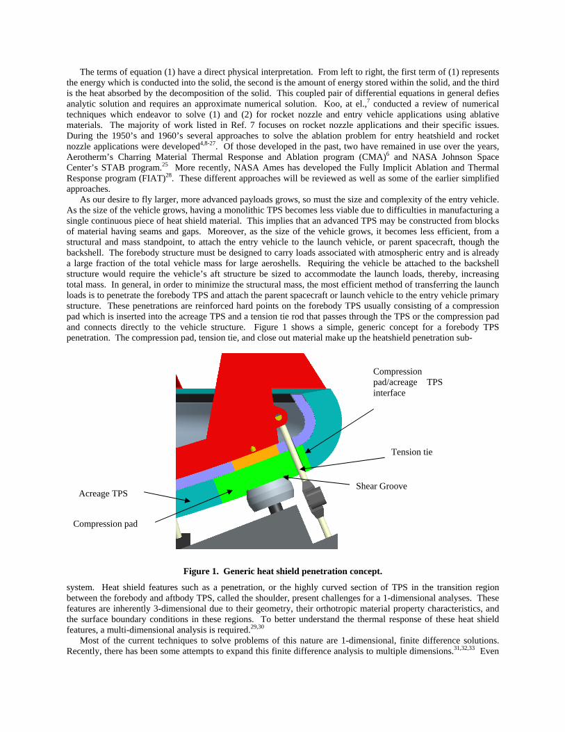
The terms of equation (1) have a direct physical interpretation. From left to right, the first term of (1) represents the energy which is conducted into the solid, the second is the amount of energy stored within the solid, and the third is the heat absorbed by the decomposition of the solid. This coupled pair of differential equations in general defies analytic solution and requires an approximate numerical solution. Koo, at el.,7 conducted a review of numerical techniques which endeavor to solve (1) and (2) for rocket nozzle and entry vehicle applications using ablative materials. The majority of work listed in Ref. 7 focuses on rocket nozzle applications and their specific issues. During the 1950’s and 1960’s several approaches to solve the ablation problem for entry heatshield and rocket nozzle applications were developed4,8-27. Of those developed in the past, two have remained in use over the years, Aerotherm’s Charring Material Thermal Response and Ablation program (CMA)6 and NASA Johnson Space Center’s STAB program.25 More recently, NASA Ames has developed the Fully Implicit Ablation and Thermal Response program (FIAT)28. These different approaches will be reviewed as well as some of the earlier simplified approaches. As our desire to fly larger, more advanced payloads grows, so must the size and complexity of the entry vehicle. As the size of the vehicle grows, having a monolithic TPS becomes less viable due to difficulties in manufacturing a single continuous piece of heat shield material. This implies that an advanced TPS may be constructed from blocks of material having seams and gaps. Moreover, as the size of the vehicle grows, it becomes less efficient, from a structural and mass standpoint, to attach the entry vehicle to the launch vehicle, or parent spacecraft, though the backshell. The forebody structure must be designed to carry loads associated with atmospheric entry and is already a large fraction of the total vehicle mass for large aeroshells. Requiring the vehicle be attached to the backshell structure would require the vehicle’s aft structure be sized to accommodate the launch loads, thereby, increasing total mass. In general, in order to minimize the structural mass, the most efficient method of transferring the launch loads is to penetrate the forebody TPS and attach the parent spacecraft or launch vehicle to the entry vehicle primary structure. These penetrations are reinforced hard points on the forebody TPS usually consisting of a compression pad which is inserted into the acreage TPS and a tension tie rod that passes through the TPS or the compression pad and connects directly to the vehicle structure. Figure 1 shows a simple, generic concept for a forebody TPS penetration. The compression pad, tension tie, and close out material make up the heatshield penetration sub-

Figure 1. Generic heat shield penetration concept.

system. Heat shield features such as a penetration, or the highly curved section of TPS in the transition region between the forebody and aftbody TPS, called the shoulder, present challenges for a 1-dimensional analyses. These features are inherently 3-dimensional due to their geometry, their orthotropic material property characteristics, and the surface boundary conditions in these regions. To better understand the thermal response of these heat shield features, a multi-dimensional analysis is required.29,30

Most of the current techniques to solve problems of this nature are 1-dimensional, finite difference solutions. Recently, there has been some attempts to expand this finite difference analysis to multiple dimensions.31,32,33 Even

Acreage TPS

Tension tie

Compression pad

Compression pad/acreage TPS interface

Shear Groove

with a multi-dimensional finite difference tool, there is very little synergy between the actual heatshield, or compression pad design, and the analysis. Most of the current 1-dimensional tools require the user to greatly simplify the geometry, generate the mesh by hand, and run the analysis. There is no direct way to feed those results back to the geometry for incorporation into a thermo-structural analysis, or for just simply to display the results on the actual geometry for post processing. A thermal response analysis tool that is compatible with modern design and analysis tools has the potential to break the barriers that exist between the design, which includes the TPS material and its structure, and the analysis, which includes the thermal and structural characterization of the system. A large number of modern analysis tools make use of a finite element discretization of complex geometry which was generated by a 3-dimensional CAD program. Therefore, any new tool developed should be 3-dimensional as well as make use of the finite element discretization generated by these tools. Using the finite element mesh generated by one of these modern design and analysis tools maintains the synergy between the two since the results can be easily mapped back to the original geometry for use in subsequent analyses, or for post processing vizualization. The work presented in this paper is the first step in moving towards a modern 3-dimensional thermal response and analysis tool which solves the problem described by the general equations given in (1) and (2). Before any discussion is made about the current finite element solution, it is prudent to review the most prominent past and present finite difference solutions to the system of equations given in (1) and (2).

II. Review of Past and Current Approaches to Solve the Ablation Problem

Early attempts in the 1950’s and early 60’s at solving the thermochemical ablation problem presented in general by equations (1) and (2) involved coupling a simple 1-dimensionl heat conduction calculation with no decomposition or pyrolysis gas flow with the heat of ablation to predict surface recession.4,5,13,22,34 The heat of ablation, or Q*, as it is denoted in the literature, is often incorrectly used as a material property, when in fact it is only a data correlation parameter valid only during steady state ablation. For these early formulations the 1-D heat equation for the in-depth temperatures was given by equation (3). For these early formulations, researchers developed an energy balance equation at the surface to describe phenomenon that they knew about. The surface energy balance used is given by equation (4).

pT Tc kt x x

ρ ∂ ∂ ∂⎛ ⎞= ⎜ ⎟∂ ∂ ∂⎝ ⎠ (3)

( )4w

w

TTr air

cw w v r airr

H HTk q T s H s H Hx H

σε ρ ρ η⎛ ⎞−∂

− = − + + Δ + −⎜ ⎟∂ ⎝ ⎠& & & (4)

The left hand side of equation (4) is the net conductive heat flux from the surface and provides the link to the in-depth energy equation. The first term on the right hand side of (4) represents the net convective heat flux into the surface in the absence of ablation, the second term is the net radiative heat flux away from the surface, the third represents the energy absorbed by material vaporization at the surface, and the last term represents the energy flux absorbed due to transpiration of the ablation products into the boundary layer. By making the approximation that the ablation is a steady state process it can be shown that the heat flux conducted into the material can be represented by equation (5). Substituting equation (5) into equation (4), rearranging and grouping similar terms the surface

0( )p wss

Tk sc T Tx

ρ∂= −

∂& (5)

energy equation for steady state ablation is obtained and given by equation (6). If equation (6) is divided by the

( )4wT

r aircw w p v

r

H Hq T s c T H HH

σε ρ η⎛ ⎞−

− = Δ + Δ + Δ⎜ ⎟⎝ ⎠

& & (6)

density and recession rate all of the parameters on the right hand side are either known or can be measured in an arc jet test. The resulting equation is definition of the thermochemical heat of ablation and is given in equation (7).

4

*

wTr air

cw wr

p v

H Hq TH

Q c T H Hs

σεη

ρ

⎛ ⎞−−⎜ ⎟

⎝ ⎠= = Δ + Δ + Δ&

& (7)

Examination of equation (7) shows that Q* is linear in ΔH, consequently it was correlated to arc jet data and tabulated as a function of ΔH. Plotting the data the slope of the resulting line was taken a η and the y-intercept was taken as p vc T HΔ + Δ . Since the specific heat and temperature are known or could be determined from a test, ΔHv could also be derived. Equation (4) could then be used as the surface energy balance coupled to a transient conduction solution with the additional constraint that the recession rate was equal to zero until a specified ablation temperature was reached. In 1961, Munson and Spindler23 introduced in-depth thermal response modeling for organic resin composite materials which would decompose in-depth. Their formulation for the in-depth conduction is given by equation (8) and their surface energy balance was given by (9).

gp p d

T T Tc k c m Ht x x x t

ρρ ∂ ∂ ∂ ∂ ∂⎛ ⎞= − + Δ⎜ ⎟∂ ∂ ∂ ∂ ∂⎝ ⎠& (8)

( )1 2

41 2hw w v v

w

Tq T k s f H f Hx

φ σε ρ∂⎛ ⎞− = + Δ + Δ⎜ ⎟∂⎝ ⎠& & (9)

Where the pyrolysis gas mass flux, decomposition rate and the transpiration correction, , ,tm andρ φ∂∂& respectively

where given by equations (10).

( )

( ) ( )

( , ) ( , )

( , ) ( , ) exp( , )

exp (1 ) ,

l

x

nr

s w g s

cw

m x t x t dxt

Bx t A x tt T x t

s m hf f where f

q

ρ

ρ ρ ρ

η ρ ηφ α

∂=

∂

⎛ ⎞∂ −= − ⎜ ⎟∂ ⎝ ⎠

+= − + =

∫&

& &

&

(10)

A more rigorous approach introduced by Kratsch, Hearne, and McChesney20 in 1963, modeled the decomposition as a mixture of organic resin and fiber reinforcement given in equation (11).

(1 )s resin fiberρ ρ ρ= Γ + − Γ (11)

The in-depth equation Kratsch, et. al. used was similar to that used by Munson and Spindler, but they recognized that some parameters involved complex chemical processes and should be expressed in terms of the enthalpy shown in equation (12).

( )( )s s sg g d

H Tk m H Ht y y y t

ρ ρ⎡ ⎤∂ ∂∂ ∂ ∂= + + Δ⎢ ⎥∂ ∂ ∂ ∂ ∂⎣ ⎦

& (12)

Kratch et. Al. also adopted the transfer coefficient approach developed by Lees35 to approximate the heat transfer to the ablating surface from the chemically reacting boundary layer. Lees showed that the surface energy balance for an ablating material in a chemically reacting boundary layer could be written as shown in equation (13).

( ) ( )* * 0

( )

e e H sr sw e e M ie iw i c c g gi

w w rad radout in

dTk U C H h U C Z Z h m h m hdx

v h q q

ρ ρ

ρ α

− = − + − + +

− + −

∑ & &

(13)

Assuming that the heat and mass transfer coefficients are equal and the Lewis and Prandtl numbers are unity, and defining non-dimensional ablation rates shown in equation (14), the surface energy balance can be written as shown in equation (15).

( ) , ,gw c

g ce e M e e M e e M

mv mB B BU C U C U Cρ

ρ ρ ρ′ ′ ′= = =

& & (14)

( ) *e e H sr sw c c g g w rad rad

out in

dTk U C H h B h B h B h q q qdx

ρ α′ ′ ′− = − + + − − + − (15)

In the mid to late 60’s, Kendall, Rindal, and Bartlett36, and Moyer and Rindal6 extended the work by Kratsch et. al. to include unequal heat and mass transfer coefficients and non-unity Lewis and Prandtl numbers. They also included the work of Goldstein37 which characterized the decomposition of organic resin composites using a three reaction Arrhenius equation model. They also corrected the in-depth energy equation to account for the energy of the pyrolysis gas convection and generation within the solid and also corrected it to account for grid motion due to a coordinate system that is attached to the receding surface. Their form of the in-depth energy equation is given in equation (16). Kendall, Rindal, Moyer, and Bartlett were the primary authors of CMA. CMA has stood the test of time and is still widely used in industry, academia, and government.

( ) gp g p g

xS S S S

hT T Tc k h h S c mt x x t x x

ρρ ρ∂⎛ ⎞∂ ∂ ∂ ∂ ∂

= + − + +⎜ ⎟∂ ∂ ∂ ∂ ∂ ∂⎝ ⎠& & (16)

Until the late 1990’s no significant development was done on the analysis of ablative thermal protection systems. In 1999 NASA Ames updated the codes developed by Aerotherm. Chen and Milos28 wrote FIAT. FIAT uses the same fundamental theory as CMA but the solution scheme is fully implicit and enhances the stability and convergence. FIAT also has other useful features such as a material database, automated mesh generation, and thickness optimization. FIAT is now the main analysis code being used to design the Orion Crew Exploration Vehicle heatshield.

A. Finite Difference versus the Finite Element Method

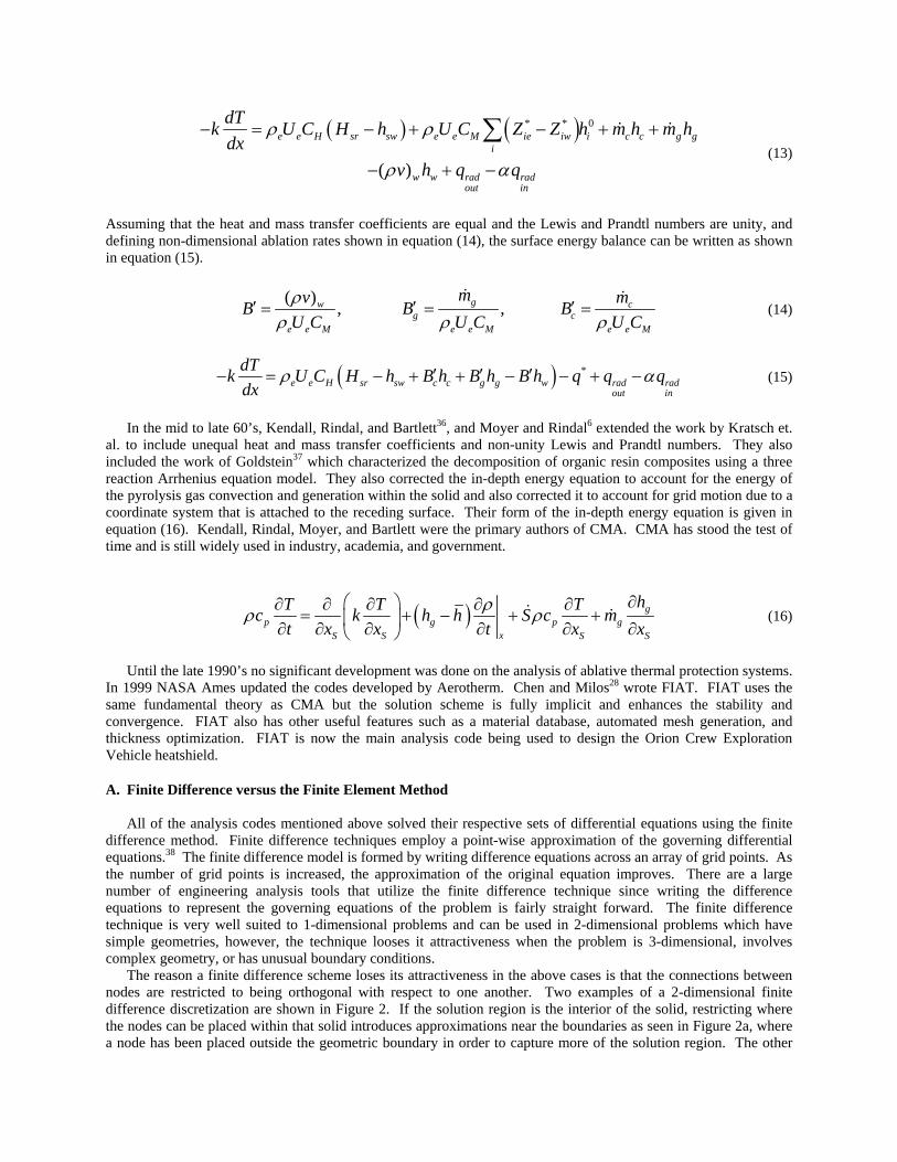
All of the analysis codes mentioned above solved their respective sets of differential equations using the finite difference method. Finite difference techniques employ a point-wise approximation of the governing differential equations.38 The finite difference model is formed by writing difference equations across an array of grid points. As the number of grid points is increased, the approximation of the original equation improves. There are a large number of engineering analysis tools that utilize the finite difference technique since writing the difference equations to represent the governing equations of the problem is fairly straight forward. The finite difference technique is very well suited to 1-dimensional problems and can be used in 2-dimensional problems which have simple geometries, however, the technique looses it attractiveness when the problem is 3-dimensional, involves complex geometry, or has unusual boundary conditions. The reason a finite difference scheme loses its attractiveness in the above cases is that the connections between nodes are restricted to being orthogonal with respect to one another. Two examples of a 2-dimensional finite difference discretization are shown in Figure 2. If the solution region is the interior of the solid, restricting where the nodes can be placed within that solid introduces approximations near the boundaries as seen in Figure 2a, where a node has been placed outside the geometric boundary in order to capture more of the solution region. The other

option available is to remove that node and leave a portion of the solid out of the solution region, shown in Figure 2b. This “stair stepping”, as it is commonly called, in addition to not exactly representing the geometry, also makes it difficult to apply an accurate boundary condition to the curved boundary of the solid. The same type of problem exists for fluid flow problems as well and all finite difference formulations in general. In order to minimize the approximations on the boundaries, a finite difference mesh would need have an increased number of nodes in those areas. Increasing the number of nodes increases the computational time necessary to obtain a solution.

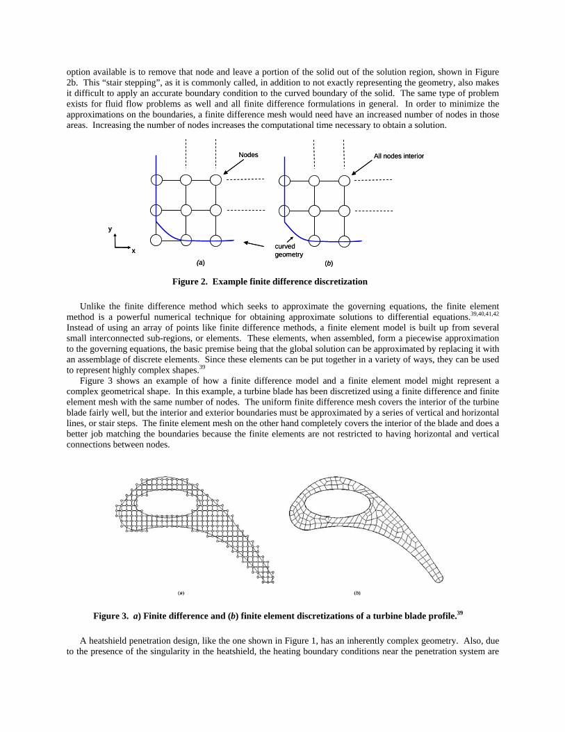
Unlike the finite difference method which seeks to approximate the governing equations, the finite element method is a powerful numerical technique for obtaining approximate solutions to differential equations.39,40,41,42 Instead of using an array of points like finite difference methods, a finite element model is built up from several small interconnected sub-regions, or elements. These elements, when assembled, form a piecewise approximation to the governing equations, the basic premise being that the global solution can be approximated by replacing it with an assemblage of discrete elements. Since these elements can be put together in a variety of ways, they can be used to represent highly complex shapes.39 Figure 3 shows an example of how a finite difference model and a finite element model might represent a complex geometrical shape. In this example, a turbine blade has been discretized using a finite difference and finite element mesh with the same number of nodes. The uniform finite difference mesh covers the interior of the turbine blade fairly well, but the interior and exterior boundaries must be approximated by a series of vertical and horizontal lines, or stair steps. The finite element mesh on the other hand completely covers the interior of the blade and does a better job matching the boundaries because the finite elements are not restricted to having horizontal and vertical connections between nodes.

A heatshield penetration design, like the one shown in Figure 1, has an inherently complex geometry. Also, due to the presence of the singularity in the heatshield, the heating boundary conditions near the penetration system are

y

x

All nodes interior

curved geometry

(b)

Nodes

(a)

y

x

y

x

All nodes interior

curved geometry

(b)

Nodes

(a) Figure 2. Example finite difference discretization

Figure 3. a) Finite difference and (b) finite element discretizations of a turbine blade profile.39

complex and vary significantly across the surface of the penetration. These are two of the reasons that a finite element solution of the governing differential equations is sought for the thermal response of the penetration subsystem. Another reason for seeking a finite element solution is compatibility with modern design and analysis tools which will be discussed below.

B. The Need for a Three Dimensional Ablative Thermal Response Analysis Capability

For some types of problems a 1-dimensional solution may not capture all of the details necessary to fully describe the thermal response of a particular geometry or material. Regions where the geometry is highly curved, there are high temperature gradients and the in-plane thermal conductivity is significant, and pyrolysis gas flow may not be normal to the heated surface, are examples where a 1-dimensional solution is inadequate. Researchers in the 1960’s recognized the importance of multi-dimensional effects in rocket nozzles where the geometry is highly curved, multiple materials may exist in the cross sectional plane, and high temperature gradients with significant in-plane conduction are observed.29,30 Although the work presented in these two references was advanced from the stand point of being multi-dimensional, they lacked a general treatment of the surface energy balance. Both used heat of ablation correlation data in the form of a transpiration coefficient and a heat of vaporization term to represent the energy absorbed due to ablation. Hurwicz, et al.,29 compared 2, and 3-dimensional results with a 1-dimensional analysis of an ablative wing leading edge and a spin control fin. For the wing leading edge, they found the 1-dimensional solution over predicted the bondline temperature compared to the multi-dimensional results. For the spin control fin, they found the 1-dimensional analysis under predicted the recession.

Friedman, et.al.30, compared 2-D temperature results to rocket firing test data for an axisymmetric rocket nozzle throat. While these temperature predictions compare very well, no recession prediction was performed and as such, verification can only be performed with the test results that do not exhibit any recession.

Current efforts to analyze ablation in multi-dimensions have been successful31,32,33 but they rely on the finite difference technique to discretize the geometry. In planar problems where the high in-plane conduction demands the multi-dimensional solution, finite difference schemes are well suited. However, in problems which have complex geometry such as the shoulder region of an entry vehicle heatshield, or forebody heatshield compression pad, a finite difference scheme may not provide the best representation as shown Figure 2 and Figure 3. In Ref. 31-33, the pyrolysis gas flow is assumed to be 1-dimensional and normal to the heated surface. This assumption may not be valid where the geometry is highly curved, the virgin material is porous, or there are multiple materials in the cross sectional plane.

A 3-dimensional finite element code which utilizes the general thermochemical formulation of the ablation problem would have the ability to address the shortcomings addressed above. In addition, a finite element code would be directly compatible with modern design and analysis tools and simplify the TPS design process. Moreover, modern CFD tools are now capable of 3-dimensional solutions for the aerodynamic heating; having a 3-dimensional thermal response tool is key to being able to use those results directly. This feature becomes especially important near a compression pad, where a spatially distributed heating environment may be present. While it is true that a 3-dimensional finite element code will be more computationally intensive than the traditional 1-dimensional analysis, modern computers along with a parallel processing computational scheme should alleviate most of those challenges.

The work presented in this paper is the first step in the overall goal of developing a 3-dimensional finite element based ablative thermal response tool. In order to illustrate that the finite element method is a viable technique in solving ablation type thermal problems, a 1-dimensional ablation and thermal response code has been developed. The present tool developed here makes the same assumptions as CMA and FIAT. In particular, this 1-dimensional tool assumes that the pyrolysis gas flow is 1-dimensional and normal to the heated surface, the heat and mass transfer coefficients are equal, and that the Lewis number is unity. In addition, the pyrolysis gas formed is assumed to be in thermal equilibrium with the char and its residence time within the char is small. The decomposition is calculated explicitly as in CMA. The decomposition follows a three component Arrhenius relation as is the case for both CMA and FIAT.

III. Finite Element Formulation

The finite element formulation makes use of the governing differential equation for the in-depth thermal response developed by Moyer and Rindal6, given in equation (16) and the associated boundary conditions developed

by Kendall, Rindal, and Bartlett36 given in equation (15). The method of weighted residuals is used to derive the element equations for the finite element formulation of the thermochemical ablation problem. The method of weighted residuals is a general technique for obtaining approximate solutions to linear and non-linear partial differential equations. The first step in the method of weighted residuals is to assume a functional form of the dependent variable which satisfies the differential equation and boundary conditions. In the case of the ablation problem, the dependent variable is the temperature. Substituting this assumed function into the differential equation and boundary conditions results in an error. This error or residual is then required to vanish in an average sense over the solution domain. The averaging is done by multiplying the residual by a weighting function. The second step is to solve the equation, or equations that arise from the first step. Solving the equations developed in step one transforms the assumed function to a specific function, which becomes the sought after approximate solution. In this formulation, the Bubnov-Galerkin method, which sets the weighting functions equal to the element interpolation functions, is used to derive the element equations. Folowing the method of weighted residuals, the functional form assumed for the dependant variable and its derivative is given in equation (17) and is also shown in matrix form. The summation in (17) is performed over all

[ ] { }

[ ] { }

( ) ( )

1( ) ( )

1

nTe e

i ii

e enTi

iiS S S

T N T T N T

NT TT B Tx x x

=

=

= =

∂∂ ∂= =

∂ ∂ ∂

∑

∑ (17)

the nodes of the element. The weighted residual statement of equation (16) is written setting the weighting functions equal to the interpolation functions, Ni.

( )( )

( ) ( )

( )( ) ( )0

e

e e

gx

iee eg

p g p

Tk h hx x t

N dhT TS c m c

x x t

ρ

ρ ρΩ

⎡ ⎤⎛ ⎞∂ ∂ ∂+ − +⎢ ⎥⎜ ⎟∂ ∂ ∂⎝ ⎠⎢ ⎥ Ω =

⎢ ⎥∂∂ ∂⎢ ⎥+ −⎢ ⎥∂ ∂ ∂⎣ ⎦

∫& &

(18)

Integrating (18) by parts, noting that dΩ = dx in 1-dimension and using the definitions given in equation (17), the corresponding element equation can be written as shown in equation (19).

[ ][ ] { } [ ] [ ][ ]{ } [ ][ ]{ }

[ ] [ ] [ ] { } [ ]{ }

2 2 2

1 1 1

2 2 2

1 11

( )

( )

S S S

S S S

S S S

S SS

x x xT T

p S S p Sx x x

x x xeT T

g g S g SS x xx

c N N T dx B k B T dx S c N B T dx

TN k m B N h dx h h N dxx

ρ ρ

ρ

+ −

∂ ⎡ ⎤⎡ ⎤= + + −⎣ ⎦ ⎣ ⎦∂

∫ ∫ ∫

∫ ∫

&&

&&

(19)

The first term on the right hand side of equation (19) is evaluated at each node and results in a vector representing the net heat conducted through the element and is the link to the surface boundary conditions given by equation (15). Equation (19) can be simplified by placing it in matrix form which gives equation (20).

[ ] { } [ ] [ ]( ){ } { }( )( ) ( ) ( ) ( ) ( )ee e e e e

c sC T K K T R+ − =&& (20)

IV. Code to Code Comparison

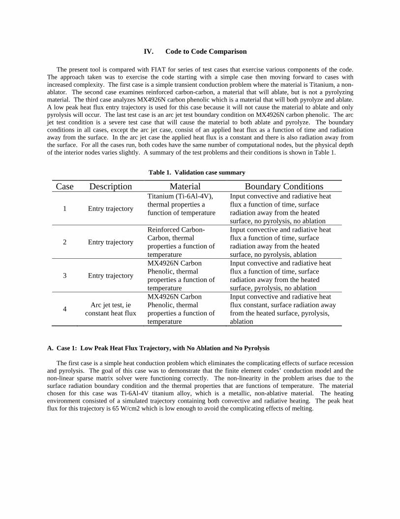
The present tool is compared with FIAT for series of test cases that exercise various components of the code. The approach taken was to exercise the code starting with a simple case then moving forward to cases with increased complexity. The first case is a simple transient conduction problem where the material is Titanium, a non-ablator. The second case examines reinforced carbon-carbon, a material that will ablate, but is not a pyrolyzing material. The third case analyzes MX4926N carbon phenolic which is a material that will both pyrolyze and ablate. A low peak heat flux entry trajectory is used for this case because it will not cause the material to ablate and only pyrolysis will occur. The last test case is an arc jet test boundary condition on MX4926N carbon phenolic. The arc jet test condition is a severe test case that will cause the material to both ablate and pyrolyze. The boundary conditions in all cases, except the arc jet case, consist of an applied heat flux as a function of time and radiation away from the surface. In the arc jet case the applied heat flux is a constant and there is also radiation away from the surface. For all the cases run, both codes have the same number of computational nodes, but the physical depth of the interior nodes varies slightly. A summary of the test problems and their conditions is shown in Table 1.

A. Case 1: Low Peak Heat Flux Trajectory, with No Ablation and No Pyrolysis

The first case is a simple heat conduction problem which eliminates the complicating effects of surface recession and pyrolysis. The goal of this case was to demonstrate that the finite element codes’ conduction model and the non-linear sparse matrix solver were functioning correctly. The non-linearity in the problem arises due to the surface radiation boundary condition and the thermal properties that are functions of temperature. The material chosen for this case was Ti-6Al-4V titanium alloy, which is a metallic, non-ablative material. The heating environment consisted of a simulated trajectory containing both convective and radiative heating. The peak heat flux for this trajectory is 65 W/cm2 which is low enough to avoid the complicating effects of melting.

Table 1. Validation case summary

Case Description Material Boundary Conditions

1 Entry trajectory

Titanium (Ti-6Al-4V), thermal properties a function of temperature

Input convective and radiative heat flux a function of time, surface radiation away from the heated surface, no pyrolysis, no ablation

2 Entry trajectory

Reinforced Carbon-Carbon, thermal properties a function of temperature

Input convective and radiative heat flux a function of time, surface radiation away from the heated surface, no pyrolysis, ablation

3 Entry trajectory

MX4926N Carbon Phenolic, thermal properties a function of temperature

Input convective and radiative heat flux a function of time, surface radiation away from the heated surface, pyrolysis, no ablation

4 Arc jet test, ie constant heat flux

MX4926N Carbon Phenolic, thermal properties a function of temperature

Input convective and radiative heat flux constant, surface radiation away from the heated surface, pyrolysis, ablation

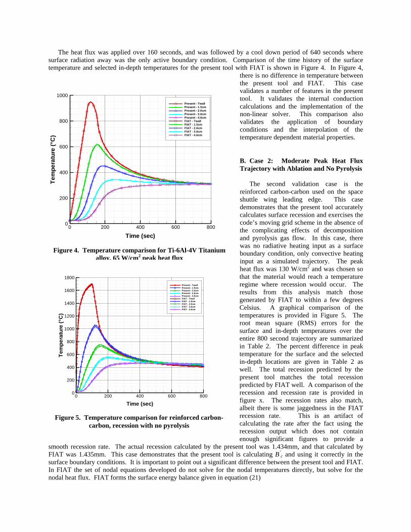
The heat flux was applied over 160 seconds, and was followed by a cool down period of 640 seconds where surface radiation away was the only active boundary condition. Comparison of the time history of the surface temperature and selected in-depth temperatures for the present tool with FIAT is shown in Figure 4. In Figure 4,

there is no difference in temperature between the present tool and FIAT. This case validates a number of features in the present tool. It validates the internal conduction calculations and the implementation of the non-linear solver. This comparison also validates the application of boundary conditions and the interpolation of the temperature dependent material properties.

B. Case 2: Moderate Peak Heat Flux Trajectory with Ablation and No Pyrolysis The second validation case is the reinforced carbon-carbon used on the space shuttle wing leading edge. This case demonstrates that the present tool accurately calculates surface recession and exercises the code’s moving grid scheme in the absence of the complicating effects of decomposition and pyrolysis gas flow. In this case, there was no radiative heating input as a surface boundary condition, only convective heating input as a simulated trajectory. The peak heat flux was 130 W/cm2 and was chosen so that the material would reach a temperature regime where recession would occur. The results from this analysis match those generated by FIAT to within a few degrees Celsius. A graphical comparison of the temperatures is provided in Figure 5. The root mean square (RMS) errors for the surface and in-depth temperatures over the entire 800 second trajectory are summarized in Table 2. The percent difference in peak temperature for the surface and the selected in-depth locations are given in Table 2 as well. The total recession predicted by the present tool matches the total recession predicted by FIAT well. A comparison of the recession and recession rate is provided in figure x. The recession rates also match, albeit there is some jaggedness in the FIAT recession rate. This is an artifact of calculating the rate after the fact using the recession output which does not contain enough significant figures to provide a

smooth recession rate. The actual recession calculated by the present tool was 1.434mm, and that calculated by FIAT was 1.435mm. This case demonstrates that the present tool is calculating B’

c and using it correctly in the surface boundary conditions. It is important to point out a significant difference between the present tool and FIAT. In FIAT the set of nodal equations developed do not solve for the nodal temperatures directly, but solve for the nodal heat flux. FIAT forms the surface energy balance given in equation (21)

Time (sec)

Tem

pera

ture

(°C

)

0 200 400 600 8000

200

400

600

800

1000Present - TwallPresent - 1.5cmPresent - 2.6cmPresent - 3.6cmPresent - 4.6cmFIAT - TwallFIAT - 1.5cmFIAT - 2.6cmFIAT - 3.6cmFIAT - 4.6cm

Figure 4. Temperature comparison for Ti-6Al-4V Titanium

alloy, 65 W/cm2 peak heat flux

Time (sec)

Tem

pera

ture

(°C

)

0 200 400 600 8000

200

400

600

800

1000

1200

1400

1600

1800Present - TwallPresent - 1.5cmPresent - 2.6cmPresent - 3.6cmPresent - 4.6cmFIAT - TwallFIAT - 1.5cmFIAT - 2.6cmFIAT - 3.6cmFIAT - 4.6cm

Figure 5. Temperature comparison for reinforced carbon-

carbon, recession with no pyrolysis

( ) *e e H sr sw c c g g w rad rad

out in

dTk U C H h B h B h B h q q qdx

ρ α′ ′ ′− = − + + − − + − (21)

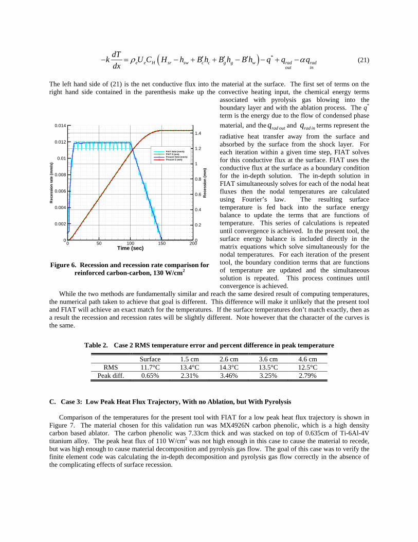
The left hand side of (21) is the net conductive flux into the material at the surface. The first set of terms on the right hand side contained in the parenthesis make up the convective heating input, the chemical energy terms

associated with pyrolysis gas blowing into the boundary layer and with the ablation process. The q* term is the energy due to the flow of condensed phase material, and the rad outq and rad inq terms represent the radiative heat transfer away from the surface and absorbed by the surface from the shock layer. For each iteration within a given time step, FIAT solves for this conductive flux at the surface. FIAT uses the conductive flux at the surface as a boundary condition for the in-depth solution. The in-depth solution in FIAT simultaneously solves for each of the nodal heat fluxes then the nodal temperatures are calculated using Fourier’s law. The resulting surface temperature is fed back into the surface energy balance to update the terms that are functions of temperature. This series of calculations is repeated until convergence is achieved. In the present tool, the surface energy balance is included directly in the matrix equations which solve simultaneously for the nodal temperatures. For each iteration of the present tool, the boundary condition terms that are functions of temperature are updated and the simultaneous solution is repeated. This process continues until convergence is achieved.

While the two methods are fundamentally similar and reach the same desired result of computing temperatures, the numerical path taken to achieve that goal is different. This difference will make it unlikely that the present tool and FIAT will achieve an exact match for the temperatures. If the surface temperatures don’t match exactly, then as a result the recession and recession rates will be slightly different. Note however that the character of the curves is the same.

Table 2. Case 2 RMS temperature error and percent difference in peak temperature

Surface 1.5 cm 2.6 cm 3.6 cm 4.6 cm RMS 11.7°C 13.4°C 14.3°C 13.5°C 12.5°C

Peak diff. 0.65% 2.31% 3.46% 3.25% 2.79%

C. Case 3: Low Peak Heat Flux Trajectory, With no Ablation, but With Pyrolysis

Comparison of the temperatures for the present tool with FIAT for a low peak heat flux trajectory is shown in Figure 7. The material chosen for this validation run was MX4926N carbon phenolic, which is a high density carbon based ablator. The carbon phenolic was 7.33cm thick and was stacked on top of 0.635cm of Ti-6Al-4V titanium alloy. The peak heat flux of 110 W/cm2 was not high enough in this case to cause the material to recede, but was high enough to cause material decomposition and pyrolysis gas flow. The goal of this case was to verify the finite element code was calculating the in-depth decomposition and pyrolysis gas flow correctly in the absence of the complicating effects of surface recession.

Time (sec)

Rec

essi

onra

te(m

m/s

)

Rec

essi

on(m

m)

0 50 100 150 2000

0.002

0.004

0.006

0.008

0.01

0.012

0.014

0

0.2

0.4

0.6

0.8

1

1.2

1.4

FIAT Sdot (mm/s)FIAT S (mm)Present Sdot (mm/s)Present S (mm)

Figure 6. Recession and recession rate comparison for

reinforced carbon-carbon, 130 W/cm2

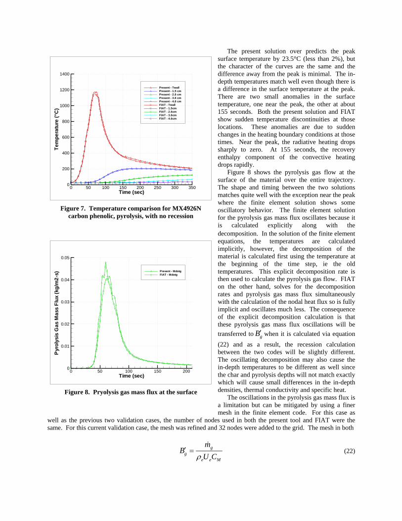
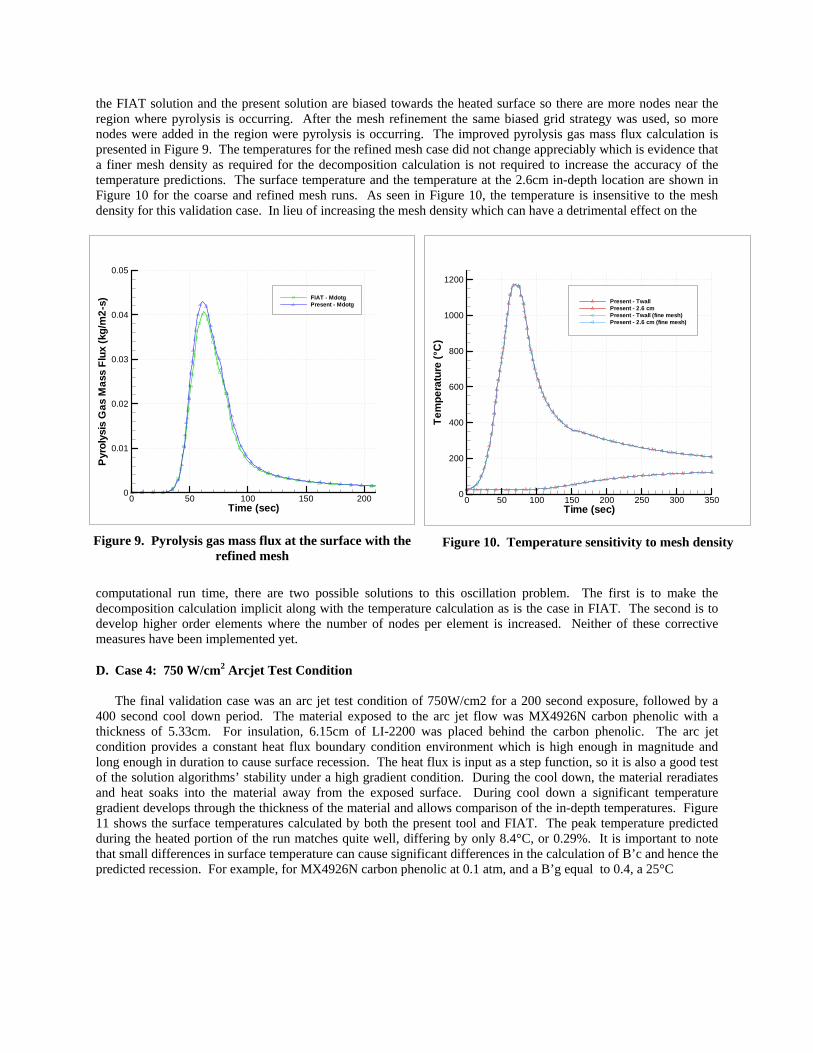
The present solution over predicts the peak surface temperature by 23.5°C (less than 2%), but the character of the curves are the same and the difference away from the peak is minimal. The in-depth temperatures match well even though there is a difference in the surface temperature at the peak. There are two small anomalies in the surface temperature, one near the peak, the other at about 155 seconds. Both the present solution and FIAT show sudden temperature discontinuities at those locations. These anomalies are due to sudden changes in the heating boundary conditions at those times. Near the peak, the radiative heating drops sharply to zero. At 155 seconds, the recovery enthalpy component of the convective heating drops rapidly. Figure 8 shows the pyrolysis gas flow at the surface of the material over the entire trajectory. The shape and timing between the two solutions matches quite well with the exception near the peak where the finite element solution shows some oscillatory behavior. The finite element solution for the pyrolysis gas mass flux oscillates because it is calculated explicitly along with the decomposition. In the solution of the finite element equations, the temperatures are calculated implicitly, however, the decomposition of the material is calculated first using the temperature at the beginning of the time step, ie the old temperatures. This explicit decomposition rate is then used to calculate the pyrolysis gas flow. FIAT on the other hand, solves for the decomposition rates and pyrolysis gas mass flux simultaneously with the calculation of the nodal heat flux so is fully implicit and oscillates much less. The consequence of the explicit decomposition calculation is that these pyrolysis gas mass flux oscillations will be transferred to gB′ when it is calculated via equation (22) and as a result, the recession calculation between the two codes will be slightly different. The oscillating decomposition may also cause the in-depth temperatures to be different as well since the char and pyrolysis depths will not match exactly which will cause small differences in the in-depth densities, thermal conductivity and specific heat. The oscillations in the pyrolysis gas mass flux is a limitation but can be mitigated by using a finer mesh in the finite element code. For this case as

well as the previous two validation cases, the number of nodes used in both the present tool and FIAT were the same. For this current validation case, the mesh was refined and 32 nodes were added to the grid. The mesh in both

gg

e e M

mB

U Cρ′ =

& (22)

Time (sec)

Tem

pera

ture

(°C

)

0 50 100 150 200 250 300 3500

200

400

600

800

1000

1200

1400

Present - TwallPresent - 1.5 cmPresent - 2.6 cmPresent - 3.6 cmPresent - 4.6 cmFIAT - TwallFIAT - 1.5cmFIAT - 2.6cmFIAT - 3.6cmFIAT - 4.6cm

Figure 7. Temperature comparison for MX4926N

carbon phenolic, pyrolysis, with no recession

Time (sec)

Pyr

olys

isG

asM

ass

Flux

(kg/

m2-

s)

0 50 100 150 2000

0.01

0.02

0.03

0.04

0.05

Present - MdotgFIAT - Mdotg

Figure 8. Pryolysis gas mass flux at the surface

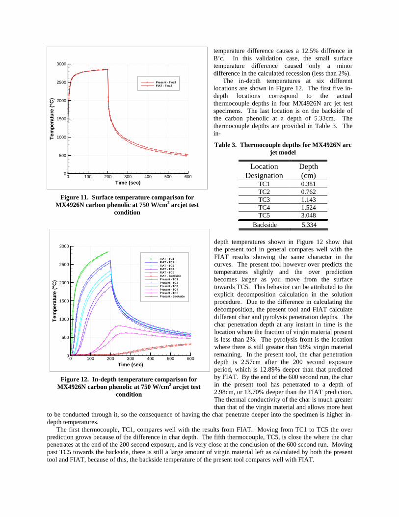
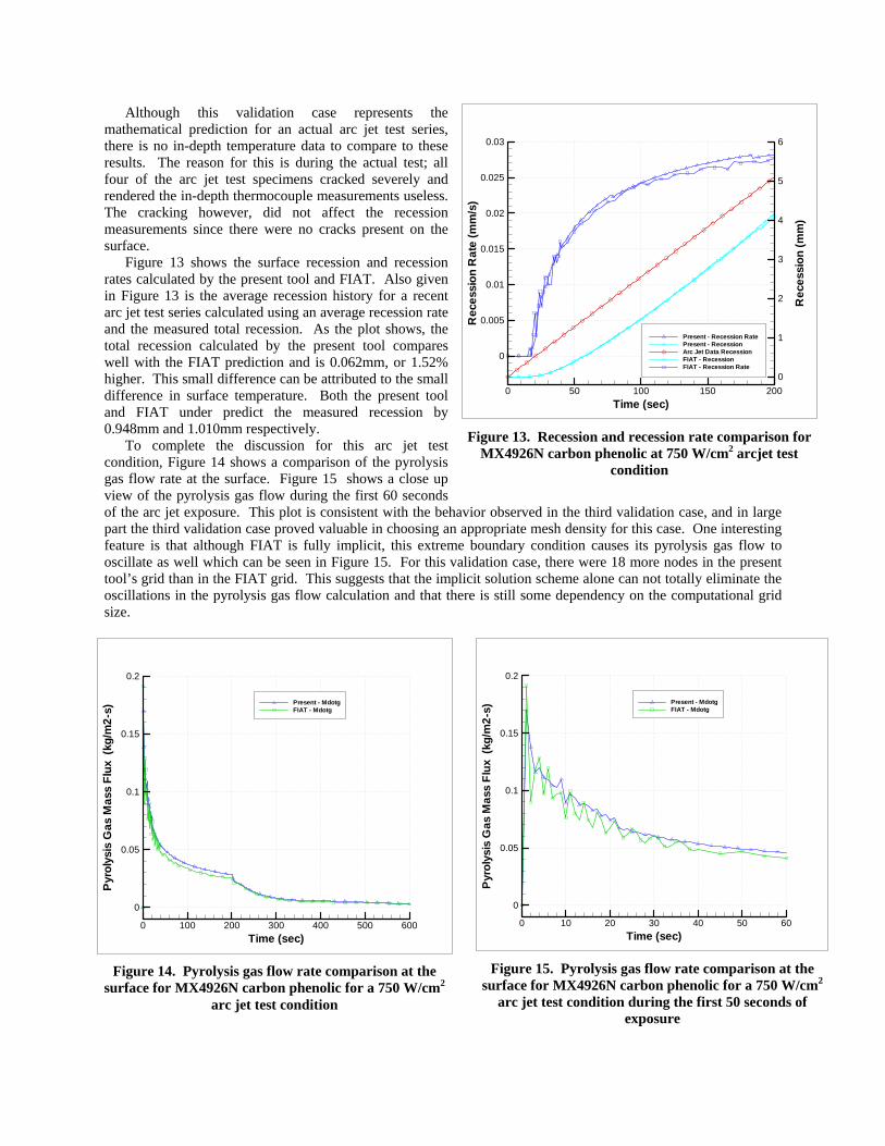
the FIAT solution and the present solution are biased towards the heated surface so there are more nodes near the region where pyrolysis is occurring. After the mesh refinement the same biased grid strategy was used, so more nodes were added in the region were pyrolysis is occurring. The improved pyrolysis gas mass flux calculation is presented in Figure 9. The temperatures for the refined mesh case did not change appreciably which is evidence that a finer mesh density as required for the decomposition calculation is not required to increase the accuracy of the temperature predictions. The surface temperature and the temperature at the 2.6cm in-depth location are shown in Figure 10 for the coarse and refined mesh runs. As seen in Figure 10, the temperature is insensitive to the mesh density for this validation case. In lieu of increasing the mesh density which can have a detrimental effect on the

computational run time, there are two possible solutions to this oscillation problem. The first is to make the decomposition calculation implicit along with the temperature calculation as is the case in FIAT. The second is to develop higher order elements where the number of nodes per element is increased. Neither of these corrective measures have been implemented yet.

D. Case 4: 750 W/cm2 Arcjet Test Condition

The final validation case was an arc jet test condition of 750W/cm2 for a 200 second exposure, followed by a 400 second cool down period. The material exposed to the arc jet flow was MX4926N carbon phenolic with a thickness of 5.33cm. For insulation, 6.15cm of LI-2200 was placed behind the carbon phenolic. The arc jet condition provides a constant heat flux boundary condition environment which is high enough in magnitude and long enough in duration to cause surface recession. The heat flux is input as a step function, so it is also a good test of the solution algorithms’ stability under a high gradient condition. During the cool down, the material reradiates and heat soaks into the material away from the exposed surface. During cool down a significant temperature gradient develops through the thickness of the material and allows comparison of the in-depth temperatures. Figure 11 shows the surface temperatures calculated by both the present tool and FIAT. The peak temperature predicted during the heated portion of the run matches quite well, differing by only 8.4°C, or 0.29%. It is important to note that small differences in surface temperature can cause significant differences in the calculation of B’c and hence the predicted recession. For example, for MX4926N carbon phenolic at 0.1 atm, and a B’g equal to 0.4, a 25°C

Time (sec)

Pyr

olys

isG

asM

ass

Flux

(kg/

m2-

s)

0 50 100 150 2000

0.01

0.02

0.03

0.04

0.05

FIAT - MdotgPresent - Mdotg

Figure 9. Pyrolysis gas mass flux at the surface with the

refined mesh

Time (sec)

Tem

pera

ture

(°C

)

0 50 100 150 200 250 300 3500

200

400

600

800

1000

1200

Present - TwallPresent - 2.6 cmPresent - Twall (fine mesh)Present - 2.6 cm (fine mesh)

Figure 10. Temperature sensitivity to mesh density

temperature difference causes a 12.5% diffrence in B’c. In this validation case, the small surface temperature difference caused only a minor difference in the calculated recession (less than 2%). The in-depth temperatures at six different locations are shown in Figure 12. The first five in-depth locations correspond to the actual thermocouple depths in four MX4926N arc jet test specimens. The last location is on the backside of the carbon phenolic at a depth of 5.33cm. The thermocouple depths are provided in Table 3. The in-

Table 3. Thermocouple depths for MX4926N arc jet model

Location Designation

Depth (cm)

TC1 0.381 TC2 0.762 TC3 1.143 TC4 1.524 TC5 3.048

Backside 5.334 depth temperatures shown in Figure 12 show that the present tool in general compares well with the FIAT results showing the same character in the curves. The present tool however over predicts the temperatures slightly and the over prediction becomes larger as you move from the surface towards TC5. This behavior can be attributed to the explicit decomposition calculation in the solution procedure. Due to the difference in calculating the decomposition, the present tool and FIAT calculate different char and pyrolysis penetration depths. The char penetration depth at any instant in time is the location where the fraction of virgin material present is less than 2%. The pyrolysis front is the location where there is still greater than 98% virgin material remaining. In the present tool, the char penetration depth is 2.57cm after the 200 second exposure period, which is 12.89% deeper than that predicted by FIAT. By the end of the 600 second run, the char in the present tool has penetrated to a depth of 2.98cm, or 13.70% deeper than the FIAT prediction. The thermal conductivity of the char is much greater than that of the virgin material and allows more heat

to be conducted through it, so the consequence of having the char penetrate deeper into the specimen is higher in-depth temperatures. The first thermocouple, TC1, compares well with the results from FIAT. Moving from TC1 to TC5 the over prediction grows because of the difference in char depth. The fifth thermocouple, TC5, is close the where the char penetrates at the end of the 200 second exposure, and is very close at the conclusion of the 600 second run. Moving past TC5 towards the backside, there is still a large amount of virgin material left as calculated by both the present tool and FIAT, because of this, the backside temperature of the present tool compares well with FIAT.

Time (sec)

Tem

pera

ture

(°C

)

0 100 200 300 400 500 6000

500

1000

1500

2000

2500

3000

Present - TwallFIAT - Twall

Figure 11. Surface temperature comparison for

MX4926N carbon phenolic at 750 W/cm2 arcjet test condition

Time (sec)

Tem

pera

ture

(°C

)

0 100 200 300 400 500 6000

500

1000

1500

2000

2500

3000

FIAT - TC1FIAT - TC2FIAT - TC3FIAT - TC4FIAT - TC5FIAT - BacksidePresent - TC1Present - TC2Present - TC3Present - TC4Present - TC5Present - Backside

Figure 12. In-depth temperature comparison for

MX4926N carbon phenolic at 750 W/cm2 arcjet test condition

Although this validation case represents the mathematical prediction for an actual arc jet test series, there is no in-depth temperature data to compare to these results. The reason for this is during the actual test; all four of the arc jet test specimens cracked severely and rendered the in-depth thermocouple measurements useless. The cracking however, did not affect the recession measurements since there were no cracks present on the surface. Figure 13 shows the surface recession and recession rates calculated by the present tool and FIAT. Also given in Figure 13 is the average recession history for a recent arc jet test series calculated using an average recession rate and the measured total recession. As the plot shows, the total recession calculated by the present tool compares well with the FIAT prediction and is 0.062mm, or 1.52% higher. This small difference can be attributed to the small difference in surface temperature. Both the present tool and FIAT under predict the measured recession by 0.948mm and 1.010mm respectively. To complete the discussion for this arc jet test condition, Figure 14 shows a comparison of the pyrolysis gas flow rate at the surface. Figure 15 shows a close up view of the pyrolysis gas flow during the first 60 seconds of the arc jet exposure. This plot is consistent with the behavior observed in the third validation case, and in large part the third validation case proved valuable in choosing an appropriate mesh density for this case. One interesting feature is that although FIAT is fully implicit, this extreme boundary condition causes its pyrolysis gas flow to oscillate as well which can be seen in Figure 15. For this validation case, there were 18 more nodes in the present tool’s grid than in the FIAT grid. This suggests that the implicit solution scheme alone can not totally eliminate the oscillations in the pyrolysis gas flow calculation and that there is still some dependency on the computational grid size.

Time (sec)

Rec

essi

onR

ate

(mm

/s)

Rec

essi

on(m

m)

0 50 100 150 200

0

0.005

0.01

0.015

0.02

0.025

0.03

0

1

2

3

4

5

6

Present - Recession RatePresent - RecessionArc Jet Data RecessionFIAT - RecessionFIAT - Recession Rate

Figure 13. Recession and recession rate comparison for

MX4926N carbon phenolic at 750 W/cm2 arcjet test condition

Time (sec)

Pyr

olys

isG

asM

ass

Flux

(kg/

m2-

s)

0 100 200 300 400 500 600

0

0.05

0.1

0.15

0.2

Present - MdotgFIAT - Mdotg

Figure 14. Pyrolysis gas flow rate comparison at the

surface for MX4926N carbon phenolic for a 750 W/cm2 arc jet test condition

Time (sec)

Pyr

olys

isG

asM

ass

Flux

(kg/

m2-

s)

0 10 20 30 40 50 60

0

0.05

0.1

0.15

0.2

Present - MdotgFIAT - Mdotg

Figure 15. Pyrolysis gas flow rate comparison at the

surface for MX4926N carbon phenolic for a 750 W/cm2 arc jet test condition during the first 50 seconds of

exposure

V. Conclusion The problem of thermochemical ablation has been reviewed and some of the more prominent past solution methods have been presented. The differences between the finite difference and finite element methods have been illustrated. The 3-dimensional character of heatshield penetration systems make them ideal for solution by the finite element method. The finite element formulation for the 1-dimensional thermochemical ablation problem has been developed and implemented in a computer tool as the first step in developing a 3-dimensional ablation and thermal response analysis tool. The 1-dimensional finite element code has been shown to compare well with the existing finite difference code FIAT. To improve the 1-D finite element code, the decomposition and pyrolysis gas flow calculations must be made implicitly as in FIAT. Another improvement to the finite element code would be to derive and implement higher order elements. Higher order elements increase the number of nodes per element and have the potential of increasing the computational efficiency by reducing the number of elements required in the solution.

VI. Acknowledgements The authors would like to acknowledge Mr. Bernie Laub, Dr. Stephen Ruffin, Dr. Vitali Volovoi, and Dr. David Schuster for their membership on Mr. Dec’s PhD. thesis committee and their review of this work. Mr. Dec would also like to thank his co-author Dr. Robert Braun for serving as his thesis committee chair.

References 1Anon., “Space Shuttle Program Thermodynamic Design Data Book,” Rockwell International, Report SD73-SH-0226,

Downey, CA, Jan. 1981. 2Scotti, S. J. (compiled by), “Current Technology for Thermal Protection Systems”, NASA-CP-3157, February 1992. 3Kratsch, K. M., Loomis, W.C., Randles, P.W., “Jupiter Probe Heatshield Design”, AIAA 1977-427, 21-23 March 1977,

AIAA/ASME 18th Structures, Structural Dynamics & Materials Conference 4Hurwicz, H., “Aerothermochemistry Studies in Ablation”, Combustion and Propulsion, 5th AGARD Colloquium on High-

Temperature Phenomena, Braunschweig, Germany, April 9-13, 1962, Pergamon Press, New York, 1963. 5Katsikas, C. J., Castle, G. K., and Higgins, J. S., “Ablation Handbook – Entry Materials Data and Design”, AFML-TR-66-

262, September 1966. 6Moyer, C. B., and Rindal, R. A., “An Analysis of the Coupled Chemically Reacting Boundary Layer and Charring Ablator –

Part II. Finite Difference Solution for the In-Depth Response of Charring Materials Considering Surface Chemical and Energy Balances”, NASA CR-1061, 1968.

7Koo, J. H., Ho, D. W. H., and Ezekoye, O. A., “A Review of Numerical and Experimental Characterization of Thermal Protection Materials – Part I. Numerical Modeling”, AIAA 2006-4936, 9-12 July 2006, 42nd Joint Propulsion Conference and Exhibit, Sacramento, CA

8Scala, S. M., “The Thermal Degradation of Reinforced Plastics During Hypersonic Re-Entry”, General Electric Company, R59SD401, July, 1959.

9Scala, S. M., “A Study of Hypersonic Ablation”, General Electric Company, RS59SD438, September, 1959. 10Scala, S. M., “The Ablation of Graphite in Dissociated Air, Part I: Theory”, General Electric Company, R62SD72,

September, 1962. 11Lafazan, S., and Siegel, B., “Ablative Thrust Chambers for Space Application”, Paper No. 5, 46th National Meeting of the

American Institute of Chemical Engineers, Los Angeles, CA., February 5th, 1962. 12Swann, R. T., and Pittman, C. M., “Numerical Analysis of the Transient Response of Advanced Thermal Protection

Systems for Atmospheric Entry”. NASA TN-D-1370, July 1962. 13Rosensweig, R. E., and Beecher, N., “Theory for the Ablation of Fiberglas Reinforced Phenolic Resin Phenolic”, AIAA

Journal, Vol. 1, No. 8, pp 1802-1809, August, 1963. 14Quinville, J. A., and Soloman, J., “Ablating Body Heat Transfer”, Aerospace Corporation, El Segundo, CA., SSD-TDR-63-

159, January 15th, 1965. 15Reinikka, E. A., and Wells, P. B., “Charring Ablators on Lifting Entry Vehicles”, Journal of Spacecraft and Rockets, Vol.

1, No. 1, January 1965. 16Swann, R. T., Dow, M. B., and Tompkins, S. S., “Analysis of the Effects of Environmental Conditions on the Performance

of Charring Ablators”, Journal of Spacecraft and Rocket, Vol. 3, No. 1, January 1966. 17Friedman, H. A., and McFarland, B. L., “Two-Dimensional Transient Ablation and Heat Conduction Analysis for Multi-

material Thrust Chamber Walls”, AIAA 1966-542, AIAA 2nd Joint Propulsion Specialist Conference, Colorado Springs, CO, June 13-17, 1966.

18Tavakoli, M. L., “An Integral Method for Analysis of the Aerothermochemical Behavior of Refractory-Fiber Reinforced Char-Forming Materials”, AIAA 1966-435, AIAA 4th Aerospace Sciences Meeting, Los Angeles, CA, June 27-29, 1966.

19Kendall, R. M., Rindal, R. A., and Bartlett, E. P., “Thermochemical Ablation”, AIAA 65-642, AIAA Thermophysics Specialist Conference, Monterey, CA, September 13-15, 1965.

20Kratsch, K. M., Hearne, L. F., and McChesney, H. R., “Thermal Performance of Heat Shield Composites During Planetary Entry”, Lockheed Missiles and Space, LMSC-803099, Sunnyvale, CA, October 1963.

21Barriault, R. J., “One-Dimensional Theory for a Model of Ablation for Plastics that Form a Charred Surface Layer”, AVCO-RAD TM-58-130, November 1958.

22Beecher, N., and Rosensweig, R. E., “Ablation Mechanisms in Plastics with Inorganic Reinforcement”, ARS Journal, Vol. 31, No. 4, April 1961, pp 530-539.

23Munson, T. R., and Spindler, R. J., “Transient Thermal Behavior of Decomposing Materials. Part I, General Theory and Application to Convective Heating”, AVCO RAD-TR-61-10, AVCO Corp., Wilmington, MA, May 1961.

24Barriault, R. J., and Yos, J., “Analysis of the Ablation of Plastic Heat Shields that Form a Charred Surface Layer”, ARS Journal, Vol. 30, No. 9, September 1960, pp. 823-829.

25Curry, D. M., “An Analysis of a Charring Ablation Thermal Protection System”, NASA TN D-3150, November 1, 1965. 26Scala, S. M., and Gilbert, L. M., “Thermal Degradation of a Char Forming Plastic During Hypersonic Flight”, ARS Journal,

Vol. 32, No. 6, June 1962, pp 917-924. 27Steg, L., and Lew, H., “Hypersonic Ablation”, The High Temperature Aspects of Hypersonic Flow, W. C. Nelson, ed.,

Proceedings of the AGARD-NATO Specialists Meeting, Rhode-Saint-Genèse, Belgium, April 3-6, 1962, MacMillian Co., New York, 1964, pp. 629-680.

28Chen, Y.-K., and Milos, F. S., “Fully Implicit Ablation and Thermal Analysis Program (FIAT),” Journal of Spacecraft and Rockets,Vol. 36, No. 3, pp 475-483, May–June 1999

29Hurwicz, H., Fifer, S., and Kelly, M., “Multidimensional Ablation and Heat Flow During Re-Entry”, Journal of Spacecraft and Rockets, Vol. 1, No. 3, May-June 1964.

30Friedman, H. A., and McFarland, B. L., “Two-Dimensional Transient Ablation and Heat Conduction Analysis for Multi-Material Thrust Chamber Walls”, AIAA-1966-542, AIAA 2nd Propulsion Joint Specialist Conference, Colorado Springs, CO, June 13-17, 1966.

31Chen, Y.-K., and Milos, F. S., “Multidimensional Effects on Heatshield Thermal Response for the Orion Crew Module”, AIAA-2007-4397, 39th AIAA Thermophysics Conference, Miami, FL, June 25-28 2007.

32Milos, F. S., and Chen, Y. –K., “Two-Dimensional Ablation, Thermal Response, and Sizing Program for Pyrolyzing Ablators”, AIAA-2008-1223, 46th AIAA Aerospace Sciences Meeting and Exhibit, Reno, NV, 7-10 January 2008.

33Chen, Y. –K., and Milos, F. S., “Three-Dimensional Ablation and Thermal Response Simulation System”, AIAA-2005-5064, 38th AIAA Thermophysics Conference, Toronto, Ontario Canada, 6-9 June 2005.

34Laub, B. and Curry, D. M. “Tutorial on Ablative TPS”, short course notes, August 2004. 35Lees, L., “Convective Heat Transfer With Mass Addition and Chemical Reactions”, Third AGARD Colloquim on

Combustion and Propulsion, Pergamon Press, New York, 1959. 36Kendall, R. M., Rindal, R. A., and Bartlett, E. P., “Thermochemical Ablation”, AIAA 65-642, AIAA Thermophysics

Specialist Conference, Monterey, CA, September 13-15, 1965. 37Goldstein, H. E., “Kinetics of Nylon and Phenolic Pyrolysis”, Lockheed Missiles and Space Company, Sunnyvale, CA.

LMSC-667876, October 1965. 38Anderson, D. A., Tannehill, J. C., and Pletcher, R. H., Computational Fluid Mechanics and Heat Transfer, Hemisphere,

Washington, DC, 1984. 39Huebner, K. H., Dewhirst, D. L., Smith, D. E., Byrom, T. G., The Finite Element Method for Engineers, 4th ed., John Wiley

& Sons, New York, 2001. 40Lewis, R. W., Nithiarasu, P., Seetharamu, K. N., Fundamentals of the Finite Element Method for Heat and Fluid Flow,

John Wiley & Sons, West Sussex, England, 2004. 41Zienkiewicz, O. C., The Finite Element Method, 3rd ed., McGraw-Hill, New York, NY, 1977. 42Reddy, J. N., and Gartling, G. K., The Finite Element Method in Heat Transfer and Fluid Dynamics, 2nd ed., CRC Press,

2000. 38Bouslog, S. A., , “Arc Jet Test Quick Look Report”,.