ABC System description for NIST SRE 2010 · ABC System description for NIST SRE 2010 May 6, 2010 1 Introduction TheABCsubmissionisacollaborationbetween: AgnitioLabs,SouthAfrica BrnoUniversityofTechnology

ABC System description for NIST SRE 2010

May 6, 2010

1 IntroductionThe ABC submission is a collaboration between:

• Agnitio Labs, South Africa

• Brno University of Technology, Czech Republic

• CRIM, Canada

We submit three different fusions of subsystems, as well as a mothballedversion of the BUT 2008 JFA system. All four submissions are exercisedonly on the core condition.

As in 2008, our efforts were directed at handling different telephone andmicrophone channels. Additionally this year, we concentrated on Englishspeech and on the special challenges posed by the new DCF weighting. Allof our development decisions were made in order to optimize for actual DCF,with the new weighting. We made no special effort to compensate our systemsfor speech of low or high vocal effort.

2 Submitted SystemsExcept for the mothballed system, our submissions are fusions of sub-systems.The fused scores are linear combinations of sub-system scores, followed by asaturating non-linearity. The combination weights, as well as two parameterscontrolling the non-linearity are numerically optimized to minimize a cross-entropy criterion, which is defined relative to the evaluation prior of 0.001.The fusion output is intended to act as a well-calibrated log-likelihood-ratio,which is thresholded at − logit(0.001) ≈ 6.9 to make hard decisions.

Some of the fusions include so-called quality measures. The quality mea-sure for a trial is computed as a weighted bilinear combination of two quality

1

vectors, one derived from the training segment, another from the test seg-ment. These combination weights are optimized simultaneously with theother fusion parameters.

We used three different development trial lists assembled from EnglishSRE 2008 data, on which we did development testing as well as optimizationof the fusion parameters. These sets were:

tel-tel: Telephone speech in both sides of the trial.

int-tel: Interview microphone speech on one side and telephone speech onthe other side of the trial.

int-int: (Courtesy of MIT) Interview microphone speech on both sides ofthe trial.

For 2010 trials, involving telephone conversations recorded on auxiliary mi-crophone, we defaulted to the fusion trained on the corresponding int-tel orint-int list.

2.1 System 1: Primary

tel-tel CRIM, BUT JFA’10, SVMCMLLR-MLLR, Agnitio I-Vector, ProsodicJFA, BUT I-Vector Full Cov, PLDA I-Vector, BUT JFA’08

int-tel CRIM, BUT JFA’10, SVM CMLLR-MLLR, BUT I-Vector Full Cov,BUT I-Vector LVCSR, PLDA I-Vector, BUT JFA’08, BUT QualityMeasures

int-int CRIM, BUT JFA’10, SVM CMLLR-MLLR, BUT I-Vector Full Cov,BUT I-Vector LVCSR, PLDA I-Vector, BUT JFA’08, BUT QualityMeasures

2.2 System 2: Contrastive

This system is the same as the primary System 1, except that:

• for tel-tel, the Agnitio Quality Measures were included,

• for int-tel and int-int, the BUT Quality Measures were excluded.

2.3 System 3: Contrastive

This system is the same as the primary System 1, except that the CRIM sub-system, which generally performed best in development testing, was removedfor all conditions.

2

2.4 System 4: Mothballed

This monolithic system is a linear calibration (without the non-linearity) ofthe BUT JFA’08 system on its own.

3 Development dataOur development data organization this year was designed specially to meetthe challenge of the new DCF. The development data was split into two(mostly) non-overlapping parts:

Sub-system training: This contains pre-2008 SRE data, as well as someSwitchboard and Fisher databases. This data is telephone and micro-phone speech in English and other languages.

Fusion training and development testing: This contains 2008 SRE and2008 SRE follow-up data, all labelled as English.

The sub-system training subset was organized and employed much as wedid in 2008, but the fusion training and development testing needed specialattention because of the new DCF.

The new DCF weights false-alarms 1000 times more than misses. Thisratio differs by two orders of magnitude from the old DCF weighting. Thishas two implications:

• The decision threshold becomes so high that very few, or even no false-alarms occur in the original SRE 2008 trial lists. This makes empiricalmeasurement of the false-alarm rate very unreliable.

• Duplicate pins, erroneously assigned to the same speaker in the Mixertelephone collection, caused target trials to be mislabelled as non-targets. Systems that correctly score those targets above the thresholdare then penalized with a relative weight of 1000 for each such trial.

We addressed the first problem by creating extended trial lists, with manymore non-target trials than in the original SRE trial lists. In order to decidehow many non-targets we needed, we used two methods, which mostly agreed:

• Doddington’s Rule of 30 [1], suggests there should be at least 30 false-alarms for probably approximately correct empirical false-alarm mea-surement. (The same applies to misses, but at the new DCF, theproblem usually occurs with false alarms.) We tried to make our triallists large enough so that number of false-alarms at the minimum DCFpoint of the system under evaluation exceeds 30.

3

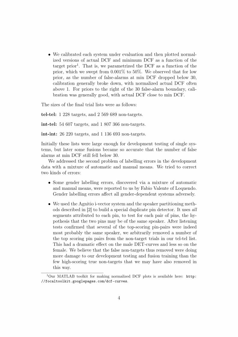
• We calibrated each system under evaluation and then plotted normal-ized versions of actual DCF and minimum DCF as a function of thetarget prior1. That is, we parametrized the DCF as a function of theprior, which we swept from 0.001% to 50%. We observed that for lowprior, as the number of false-alarms at min DCF dropped below 30,calibration generally broke down, with normalized actual DCF oftenabove 1. For priors to the right of the 30 false-alarm boundary, cali-bration was generally good, with actual DCF close to min DCF.

The sizes of the final trial lists were as follows:

tel-tel: 1 228 targets, and 2 569 689 non-targets.

int-tel: 54 607 targets, and 1 807 366 non-targets.

int-int: 26 220 targets, and 1 136 693 non-targets.

Initially these lists were large enough for development testing of single sys-tems, but later some fusions became so accurate that the number of falsealarms at min DCF still fell below 30.

We addressed the second problem of labelling errors in the developmentdata with a mixture of automatic and manual means. We tried to correcttwo kinds of errors:

• Some gender labelling errors, discovered via a mixture of automaticand manual means, were reported to us by Fabio Valente of Loquendo.Gender labelling errors affect all gender-dependent systems adversely.

• We used the Agnitio i-vector system and the speaker partitioning meth-ods described in [2] to build a special duplicate pin detector. It uses allsegments attributed to each pin, to test for each pair of pins, the hy-pothesis that the two pins may be of the same speaker. After listeningtests confirmed that several of the top-scoring pin-pairs were indeedmost probably the same speaker, we arbitrarily removed a number ofthe top scoring pin pairs from the non-target trials in our tel-tel list.This had a dramatic effect on the male DET-curves and less so on thefemale. We believe that the false non-targets thus removed were doingmore damage to our development testing and fusion training than thefew high-scoring true non-targets that we may have also removed inthis way.

1Our MATLAB toolkit for making normalized DCF plots is available here: http://focaltoolkit.googlepages.com/dcf-curves.

4

http://focaltoolkit.googlepages.com/dcf-curves

http://focaltoolkit.googlepages.com/dcf-curves

4 Sub-systemsThis section gives detailed descriptions of the various sub-systems that weused in the fusions.

4.1 BUT JFA’08

This is the configuration of the BUT JFA system as it was submitted to SRE2008, with details described below.

4.1.1 Feature Extraction

Short time gaussianized MFCC 19 + energy augmented with their deltaand double delta coefficients, making 60-dimensional feature vectors. Theanalysis window is 20 ms with a shift of 10 ms.

Short-time gaussianization uses a window of 300 frames (3 sec). For thefirst frame, only 150 frames on the right are used and the window grows till300 while we move in time. When we approach the last frame, we use only150 frames on the left side.

4.1.2 VAD

Speech/silence segmentation is performed by our Hungarian phoneme recog-nizer [3], where all phoneme classes are linked to the speech class. Segmentslabelled speech or silence are generated, but not merged yet to preservesmaller segments — a post-processing with two rules based on short timeenergy is applied first:

1. If the average energy in a speech segment is 30 dB less than the maxi-mum energy of the utterance, the segment is labelled as silence.

2. If the energy in the other channel is greater than the maximum energyminus 3 dB in the processed channel, the segment is also labelled assilence.

After this post-processing, the resulting segments are merged together. Onlyspeech segments are used. In case of 1-channel files, rule #2 is not applied.The interview data we processed as 1-channel and, we took ASR transcripts ofthe interviewer and removed his/her speech segments from our segmentationfiles based on time-stamps provided by NIST.

5

4.1.3 UBM

Two gender-dependent universal background models (UBMs) are trained onSwitchboard II Phases 2 and 3, Switchboard Cellular Parts 1 and 2, and NISTSRE 2004 and 2005 telephone data. In total, there were 16307 recordings(574 hours) from 1307 female speakers and 13229 recordings (442 hours) from1011 male speakers. We used 20 iterations of the EM algorithm and for eachwe do splitting up to 256 Gaussians and 25 iterations for 512 and up. Novariance flooring was used.

4.1.4 JFA

The Factor analysis (FA) system closely follows the description of Large Fac-tor Analysis model in Patrick Kenny’s paper [4] with MFCC19 features. Thetwo gender dependent UBMs are used to collect zero and first order statisticfor training two gender dependent FA systems.

First, for each FA system, 300 eigenvoices2 are trained on the same dataas the UBM, although only speakers with more than 8 recordings were consid-ered here. For the estimated eigenvoices, MAP estimates of speaker factorsare obtained and fixed for the following training of eigenchannels. A setof 100 eigenchannels is trained on NIST SRE 2004 and 2005 telephone data(5029 and 4187 recordings of 376 females and 294 males speaker respectively).Another set of 100 eigenchannels is trained on SRE 2005 auxiliary micro-phone data (1619 and 1322 recordings of 52 females and 45 males speakerrespectively). Another set of 20 eigenchannels is trained on SRE08 interviewdevelopment data (3 males and 3 females). All three sets are concatenatedto form final U matrix. We used linear scoring to get the final score for thetrial [5].

4.1.5 Normalization

Finally, scores are normalized using condition dependent zt-norm. For thetelephone condition we used 200 females and 200 males z-norm and t-normtelephone segments, derived each from one speaker of NIST SRE 2004,05,06data. For the interview and microphone we used together 400 utterancesfrom which 200 from interview and 200 from microphone sets were randomlychosen from NIST 2008 interview data (speakers not present in dev set) andMIX05,06 microphone data respectively.

2We refer to eigenvoices and eigenchannels following the terminology defined in [4]although these sub-spaces are estimated using the EM-algorithm, not PCA.

6

Table 1: Number of speakers per training list.set #number of speakers

znorm.int.m 17znorm.int.f 24tnorm.int.m 17tnorm.int.f 24znorm.mic.m 41znorm.mic.f 45tnorm.mic.m 39tnorm.mic.f 48znorm.tel.m 200znorm.tel.f 200tnorm.tel.m 200tnorm.tel.f 200

4.2 BUT JFA’10

This is a new configuration of the BUT JFA system, with details as describedbelow.


Short time gaussianized MFCC 19 + energy augmented with their delta anddouble delta coefficients, making 60 dimensional feature vectors. The analysiswindow has 20 ms with shift of 10 ms.


4.2.2 VAD



7



4.2.3 UBM

Two gender-dependent universal background models (UBMs) are trained onSwitchboard II Phases 2 and 3, Switchboard Cellular Parts 1 and 2, and NISTSRE 2004 and 2005 telephone data. In total, there were 16307 recordings(574 hours) from 1307 female speakers and 13229 recordings (442 hours) from1011 male speakers. We used 20 iterations of the EM algorithm and for eachwe do splitting up to 256 Gaussians and 25 iterations for 512 and up. Novariance flooring was used.

4.2.4 JFA

The Factor analysis (FA) system closely follows the description of Large Fac-tor Analysis model in Patrick Kenny’s paper [4] with MFCC19 features. Thetwo gender dependent UBMs are used to collect zero and first order statisticsfor training two gender dependent FA systems.

First, a gender dependent system aimed at telephone speech was trained,using statistics from files from NIST 200[456] and Switchboard2 Phase[23]and Switchboard Cellular Part[12]. For the female sub-system, 21663 record-ings were used, for the male-subsystem there were 16969 recordings. Bothsub-systems had 300 eigenvoices and 100 eigenchannels. The eigenchanneland eigenvoice matrices were initialized randomly and then trained with 10EM iterations of maximum likelihood and minimum divergence each. No Dmatrix was used.

Then, other eigenchannel matrices were trained (using the telephoneeigenvoice matrix) on different training data: One with 50 eigenchannels onNIST 2008 SRE interview data (2514 female recordings, 1397 male record-ings), and one with 100 eigenchannels on NIST 200[56] SRE microphone data(3702 female recordings, 2961 male recordings).

The three eigenchannel matrices (telephone, interview, and microphone)per gender were then combined to form two systems per gender: a tele-

8

phone+interview+microphone system and a telephone+microphone system.Both used the telephone eigenvoice matrix.

The telephone+interview+microphone system was used to score the int-tel and int-int conditions, the telephone+microphone system was used toscore the tel-tel conditions.

4.2.5 Normalization

Finally, scores are normalized using condition dependent zt-norm. For thetelephone condition we used 200 females and 200 males z-norm and t-normtelephone segments, derived each from one speaker of NIST SRE 2004,05,06data. For the interview and microphone we used together 400 utterancesfrom which 200 from interview and 200 from microphone sets were randomlychosen from NIST 2008 interview data (speakers not present in dev set) andMIX05,06 microphone data respectively.

See table 1.

4.3 Agnitio I-Vector

The Agnitio I-Vector system used 60-dimensional MFCC features and a 2048-component UBM to extract 400-dimensional i-vectors3 as proposed in [5, 6].The i-vectors were modelled with the two-covariance model as proposed in [2].

Score normalization is a symmetrized version of ZT-norm called S-norm.The cohorts were synthetically generated by generating normally distributedi-vectors with the between-speaker covariance.

The UBM is gender-independent, but the i-vector extractors, two-covariancemodels and score normalizations are gender-dependent. This system was de-signed for telephone speech and was run only on tel-tel trials in 2010. Forfurther details see [2].

4.4 BUT I-Vector Full Cov

This system uses 400-dimensional i-vectors extracted via 60-dimensional fea-tures and a 2048-component full-covariance UBM.

3The name i-vector is mnemonic for a vector of intermediate size (bigger than anacoustic feature vector and smaller than a supervector), which contains most of the relevantinformation about the speaker identity.

9


Short time gaussianized MFCC 19 + energy augmented with their delta anddouble delta coefficients, making 60 dimensional feature vectors. The analysiswindow has 20 ms with shift of 10 ms.


4.4.2 VAD





4.4.3 UBM

One gender-independent universal background model was represented as afull covariance, 2048-component GMM. It was trained on the NIST SRE 2004and 2005 telephone data (376 female speakers in 171 hours of speech, 294male speakers in 138 hours of speech). Variance flooring was applied in eachiteration, where the threshold was computed as an average variance fromeach previous iteration, scaled by 0.1.

10

4.4.4 I-vector system

I-vector system aims at modelling overall variability of the training data andcompressing the information to a low-dimensional vector. The techniqueis closely related to JFA in the sense that each training segment acts as aseparate speaker. Speaker (and/or channel) modelling techniques are thenapplied on these low-dimensional vectors. This way, an i-vector system canbe viewed as a front-end for further modelling.

To filter out the channel information from the i-vectors, LDA was usedas in [5]. Each trial score is then computed as a cosine distance between twosuch vectors.

The i-vectors extractor was trained on the following telephone data: NISTSRE 2004, NIST SRE 2005, NIST SRE 2006, Switchboard II Phases 2 and3, Switchboard Cellular Parts 1 and 2, Fisher English Parts 1 and 2 giving8396 female speaker in 1463 hours of speech, and 6168 male speakers in 1098hours of speech (both after VAD).

The tel-tel LDA matrix was trained on the same data as the i-vectorextractor, except the Fisher data was excluded, resulting in 1684 femalespeakers in 715 hours of speech and 1270 male speakers in 537 hours ofspeech. The int-tel and int-int LDA matrices were trained on the samedata as tel-tel, augmented with all possible microphone and interview data,resulting in 1830 female speakers in 832 hours of speech and 1387 speakersin 621 hours of speech.

4.4.5 Normalization

Simplified symmetrical normalization—s-norm—is applied to the scores: Foreach trial, the enrolled model and the test segment (both represented by ani-vector) are scored against some s-norm cohort (400 speakers, gender de-pendent) and their score distributions are estimated. Two scores are thencomputed for the trial: one normalized by the enrolled model score distri-bution, and one by the test segment score distribution. The final score iscomputed as an average of the two normalized scores.

The normalization cohorts were chosen to satisfy the corresponding con-dition (e.g., interview models were normalized by telephone segments in theint-tel condition).

4.5 BUT I-Vector LVCSR

Apart from the UBM, this system is identical to the full-covariance i-vectorsystem as described in 4.4. It uses i-vectors extracted via 60-dimensional

11

features and a 2048-component diagonal-covariance UBM derived from anLVCSR system.

4.5.1 UBM

One gender-independent universal background model was represented as adiagonal covariance, 2048-component GMM. It was based on Gaussian com-ponents extracted from our LVCSR system trained on fisher (2000 hours) +300 hours from switchboard and callhome. All Gaussians were pooled to-gether, and repetitive clustering was applied to satisfy maximum likelihoodincrease in each step.

4.6 PLDA I-Vector

The system is based on the same 400-dimensional i-vectors as in the caseof the BUT I-Vector Full Cov system. However, this time the i-vectors aremodelled using a PLDA [7] model.

4.6.1 PLDA Training

The algorithms for PLDA training and scoring were implemented by Agnitio.We note that in contrast to [7], the EM-algorithm for training the PLDAmodel parameters makes use of an additional minimum-divergence update [8,9], which helps the algorithm to converge more quickly and to a generallybetter solution than plain EM.

tel-tel condition PLDA model with 90 eigenvoices and 400 eigenchannels(full rank) is trained using mixer 04,05,06 and switchboard telephonedata. No snorm is applied.

int-tel and int-int condition PLDA model with 90 eigenvoices and 400eigenchannels (full rank) is trained using pooled switchboard, mixer04,05,06 telephone and microphone data and heldout 2008 interviewdata. After the model is trained, V and D matrices are fixed and Umatrix is retrained once using telephone data, once using 05,06 micro-phone data (plus corresponding telephone recordings) and once usingheldout 2008 interview data. For scoring trials, the original matrixU (trained on everything) and the three telephone, microphone andinterview specific U matrices are stacked into one matrix of 1600 eigen-channels. No snorm is applied.

12

4.7 Prosodic JFA

4.7.1 Features

The prosodic feature generation closely follows the description in [10]. Thefeatures incorporate duration, pitch and energy measurements. Pitch andenergy values are estimated every 10 ms and energy is further normalizedby its maximum. The temporal trajectory of pitch and energy is modeledby Discrete Cosine Transformation (DCT), over a fixed frame long temporalwindow of 300 ms, with a 50 ms frame shift. The first 6 coefficients of both,transformed pitch and energy trajectories, form a fixed length feature vector.Only voiced frames (where pitch is detected) are used, all other frames are cutout prior to DCT transformation. Further, duration information is appendedas one discrete coefficient, that is the number of voiced frames within the30 frame interval.

4.7.2 Model

The Factor analysis (FA) system closely follows the description of LargeFactor Analysis model in Patrick Kenny’s paper [4]. First, gender depen-dent UBMs with 512 components each, are trained with variance flooring onSwitchboard and SRE04-06 data. After PCA initialization of V and U, 100eigenvoices are iteratively re-estimated on Switchboard and SRE04-06 data.For the tel-tel condition, we further estimate 40 eigenchannels on Switch-board and SRE04-06 data. For int-tel and int-int conditions, 10 telephonechannels are estimated on SRE04-05 data, concatenated with 10 interviewchannels, trained on SRE08 interview data and additional 10 microphonechannels, estimated on SRE05-06 microphone recordings. During verifica-tion, we use fast linear scoring [11]. All scores are further zt-normalized,using task dependent z- and t-norm lists.

4.8 SVM CMLLR-MLLR


LVCSR system was trained on 2000 hours of Fisher data + 300 hours ofSwitchboard and Callhome. The used features were PLP12_0_D_A_T(in HTK notation), with VTLN applied, and HLDA with dimensionalityreduction (52 to 39). Speaker adaptive training was done using fMPE +MPE models with crossword triphones, WER 24% on NIST eval01 task. 2-class CMLLR was used to model speech and silence, and 3-class MLLR was

13

used to model 2 data clusters and silence. From the resulting 5 matrices,only the triplet of the speech-related matrices was taken.

For MLLR and CMLLR estimation, we ran 4 iterations with intermediatedata-to-model realignment.

We did not run our own ASR recognition, rather we used the providedNIST ASR transcripts.

While phoneme alignment is estimated using VTLN features, the MLLRand CMLLR transformation matrices are estimated using non-VTLN fea-tures.

4.8.2 SVM Training

We constructed one supervector for each utterance by vectorizing one CM-LLR and two MLLR matrices. Then we applied rank normalization trainedon the NIST SRE 2004 and 2005 telephone data.

After the normalization, a Nuisance Attribute Projection (NAP) wasperformed. We computed three projection matrices: first is trained onNIST SRE 2004 and 2005 telephone data, second on NIST SRE 2005 and2006 microphone data and third is trained on NIST SRE 2008 interview data.For tel-tel system 20 dimensions from first and 10 dimensions from secondmatrix are used. For int-tel and int-int system, 20 dimensions from first,10 dimensions from second and 10 dimensions from third matrix are used.

Background data sets (data for the negative class) are constructed sepa-rately for tel-tel system and for int-tel and int-int systems.

For the tel-tel system, first all NIST SRE 2004 and 2005 telephone areused. This set is then reduced to one third by selecting the segments whichappeared most frequently as support vectors. To this reduced telephone set,the microphone data from int-tel and int-int reduced background set areadded.

For the int-tel and int-int systems, first all NIST SRE 2005 and 2006microphone data plus NIST SRE 2008 interview data were used. Then thisset was reduced to one third in the same way as for the tel-tel system. Tothis reduced microphone and interview data, the whole reduced telephoneset was added.

Finally SVM training was applied using Matlab interface for libsvm. Aprecomputed linear kernels were provided to the libsvm during the trainingand testing.

14

4.9 CRIM

This is another i-vector system, which uses a modified PLDA [7] model withheavy-tailed distributions instead of normal distributions. For details see [12]and the CRIM SRE 2010 System Description.

4.10 Agnitio Quality Measures

Quality measures are ancillary statistics computed from the input data, whichon their own contain little or no speaker discriminating information, butwhich can aid calibration of discriminative scores. In particular, if the qualitymeasures indicate that the input data is of poor quality, e.g. because of lowSNR, then the output log-likelihood-ratio can be modulated by the qualitymeasures to be close to zero. Agnitio computed two types of quality measure:

• A segment-based quality measure is a scalar value computed for eachtest segment and each train segment.

• A trial-based quality measure is a scalar value computed for everydetection trial.

The Agnitio quality measures were computed only for telephone data.

4.10.1 Segment-based Quality Measures

1. UBM state visit statistic: 12048

∑2048i=1

ni

ni+1, where ni is the expected

number of visits to UBM state i in the speech segment.

2. The average gender-dependent i-vector extractor log-likelihood, wherethe gender agrees with the NIST gender label.

3. Gender mismatch: For segments labelled male by NIST, the averagemale i-vector extractor log-likelihood, minus the average female i-vectorextractor log-likelihood. Conversely, for segments labelled female, thegender mismatch statistic is the female log-likelihood minus the malelog-likelihood.

4. The average UBM frame log-likelihood. The UBM is gender-independent.

5. The average posterior entropy for the UBM state, given the acousticframe feature vector.

6. The logarithm of the number of MFCC frames in the segment thatpassed the VAD.

15

4.10.2 Trial-based Quality measures

Both measures below were computed from the i-vector two-covariance model [2],under the assumption that the speaker in the train and test segment are thesame.

1. Channel mismatch: The squared Mahalanobis distance between thechannel variables for the two segments, where the distance is parametrizedby the within-speaker covariance, CW . The formula is δ′C−1

W δ, whereδ is the difference between the two i-vectors of the trial.

2. Speaker rarity: The expected squared Mahalanobis distance betweenthe speaker-identity variable and the origin, where the distance is parametrizedby the between-speaker covariance. The expectation is over the poste-rior for the speaker identity variable.

4.11 BUT Quality Measures

The BUT quality measures are all segment-based:

1. Gender mismatch, similar to the Agnitio ones, but computed fromMMI-trained GMMs as described below.

2. logarithm of number of frames

3. number of frames

4. SNR

5. Speech GMM log-likelihood

6. Speech+Silence GMM log-likelihood

More details are given below.

4.11.1 Gender identification likelihoods

Two likelihoods of two GMM models with 32 Gaussians. The first one wastrained only on speech frames using BUT segmentation from female speakers.The second one was trained only on speech frames using BUT segmentationfrom male speakers. The models are trained using MMI criterion, and fea-tures are MFCC_0_D_A_Z. The training data for both GMMs are fromNIST 2004 data.

16

4.11.2 GMM likelihoods

Two likelihoods of two GMM models with 256 Gaussians. The first one wastrained on only speech frames using BUT segmentation. The second onewas trained on whole files (speech and silence). The training data for bothGMMs:• 3000 randomly chosen files from MIXER 04,05,06 telephone data

• 2000 randomly chosen files from MIXER 05,06 telephone:mic data

• 1000 randomly chosen files from MIXER 08 interview data (heldoutspeakers defined by MIT).

The likelihoods are computed only for speech frames and normalized bythe number of frames.

4.11.3 SNR estimation

This SNR estimator was implemented according the article [13].

5 Fusion and calibrationThe fused and calibrated log-likelihood-ratio output for a trial with trainsegment i and test segment j is:

ìj = fε,δ(α +

N∑k=1

βksk(i, j) +M∑k=1

γkrk(i, j) + q(i)′Wq(j))

(1)

where sk(i, j) is the score of system k for the trial; rk(i, j) is the kth trial-based quality measure; q(i) and q(j) are vectors of segment-based qualitymeasures, where the vector is augmented by appending 1. The fusion pa-rameters are: offset α; linear combination weights βk and γk; the bilinearcombination matrix W, constrained to be symmetric; and the saturationparameters δ and ε. The saturating non-linearity is defined as:

fε,δ(x) = logexp(x) + exp(δ)

1 + exp(δ)− log

exp(x) + exp(−ε)1 + exp(−ε)

(2)

The saturation parameters may be interpreted as the log-odds for misla-belling in the fusion training data, respectively a target as a non-target, ora non-target as a target. If δ, ε � 0, then f is an increasing sigmoid pass-ing through the origin, with lower saturation approximately at δ and uppersaturation approximately at −ε. As the parameters approach 0 from below,the saturation levels approach 0 respectively from above and below. In ourexperiments, the optimizer typically set δ, ε ≈ −9.

17

5.1 Training

The fusion parameters were trained separately on each of the three lists ofsupervised detection trials (tel-tel, int-tel and int-int), by minimizing w.r.t.the fusion parameters the following cross-entropy objective function:

Cxe(P ) =P

T

∑(i,j)∈T

log(1 + exp(−ìj − logitP )

)+

1− PN

∑(i,j)∈N

log(1 + exp(ìj + logitP )

) (3)

where P = 0.001 to agree with the new DCF definition; T is the set of targettrials of size T ; and N the set of non-target trials of size N .

The optimization was done with the Trust-Region-Newton-Conjugate-Gradient [14, 15] optimization algorithm, which uses first and second orderpartial derivatives. The derivatives were calculated via algorithmic differ-entiation, which essentially computes derivatives of complicated functionsby applying the chain rule to combine the derivatives of simple buildingblocks [16, 17].

Although we used (3) as training objective, we evaluated our developmentresults by actual and minimum DCF. We found that in most cases, when thesaturating non-linearity was used, we got a well-calibrated actual DCF closeto minimum DCF. If we omitted the non-linearity and used a plain affinefusion transform, the actual DCF was often much higher. We conjecture thatthe non-linearity compensates both for labelling errors and data scarcity atthe challenging new DCF.

5.2 Scores and decisions

The fusion output scores are intended to act as well-calibrated log-likelihood-ratios. These scores are compared to the Bayes threshold of − logit(0.001) ≈6.9 to make hard decisions.

Although our scores can be evaluated as log-likelihood-ratios via Cllr asdefined in the evaluation plan, we optimized our scores to minimize the closelyrelated Cxe(0.001). Note that Cllr = Cxe(0.5).

6 Team membersAgnitio Niko Brümmer, Luis Buera and Edward de Villiers.

18

BUT Doris Baum, Lukáš Burget, Ondřej Glembek, Martin Karafiát, MarcelKockmann, Pavel Matějka and Oldřich Plchot.

CRIM Patrick Kenny, Pierre Ouellet and Mohammed Senoussaoui.

References[1] George R. Doddington, “Speaker recognition evaluation methodology:

a review and perspective,” in Proceedings of RLA2C, Avignon, France,Apr. 1998, pp. 60–66. 3

[2] Niko Brümmer and Edward de Villiers, “The speaker partitioning prob-lem,” in Proceedings of Speaker Odyssey 2010, Brno, Czech Republic,June 2010. 4, 9, 16

[3] Pavel Matějka, Lukáš Burget, Petr Schwarz, and Jan “Honza” Černocký,“Brno university of technology system for nist 2005 language recognitionevaluation,” in Proceedings of the IEEE Odyssey 2006 Speaker and Lan-guage Recognition Workshop, San Juan, Puerto Rico, June 2006, pp.57–64. 5, 7, 10

[4] Patrick Kenny, Pierre Ouellet, Najim Dehak, Vishwa Gupta, and PierreDumouchel, “A study of inter-speaker variability in speaker verification,”IEEE Transactions on Audio, Speech and Language Processing, July2008. 6, 8, 13

[5] Najim Dehak, Réda Dehak, Patrick Kenny, Niko Brümmer, Pierre Ouel-let, and Pierre Dumouchel, “Support vector machines versus fast scoringin the low-dimensional total variability space for speaker verification,”in Proceedings of Interspeech 2009, Brighton, UK, Sept. 2009, pp. 1559–1562. 6, 9, 11

[6] Najim Dehak, Patrick Kenny, Reda Dehak, Pierre Dumouchel, andPierre Ouellet, “Front-end factor analysis for speaker verification,” sub-mitted to IEEE Transactions on Audio, Speech and Language Process-ing, 2010. 9

[7] Simon J. D. Prince and James H. Elder, “Probabilistic linear discrimi-nant analysis for inferences about identity,” in Proceedings of 11th Inter-national Conference on Computer Vision, Rio de Janeiro, Brazil, Oct.2007. 12, 15

19

[8] Patrick Kenny, Gilles Boulianne, Pierre Ouellet, and Pierre Dumouchel,“Joint factor analysis versus eigenchannels in speaker recognition,” IEEETransactions on Audio, Speech and Language Processing, vol. 15, no. 4,pp. 1435–1447, May 2007. 12

[9] Niko Brümmer, “The em algorithm and minimum divergence,” AgnitioLabs Technical Report. Online: http://niko.brummer.googlepages.com/EMandMINDIV.pdf, Oct. 2009. 12

[10] Marcel Kockmann, Lukáš Burget, and Jan “Honza” Černocký, “Investi-gations into prosodic syllable contour features for speaker recognition,”in Proceedings of ICASSP, Dallas, United States, Mar. 2010, pp. 1–4.13

[11] Ondřej Glembek, Lukáš Burget, Najim Dehak, Niko Brümmer, andPatrick Kenny, “Comparison of scoring methods used in speaker recog-nition with Joint Factor Analysis,” in Proceedings of ICASSP, Taipei,Taiwan, Apr. 2009. 13

[12] Patrick Kenny, “Bayesian speaker verification with heavy tailed priors,”in Proceedings of Speaker Odyssey 2010, Brno, Czech Republic, June2010. 15

[13] Chanwoo Kim and Richard M. Stern, “Robust signal-to-noise ratio es-timation based on waveform amplitude distribution analysis,” in Pro-ceedings of Interspeech 2008, Brisbane, Australia, Sept. 2008. 17

[14] Jorge Nocedal and Stephen J. Wright, Numerical Optimization,Springer, 2006. 18

[15] Chih-Jen Lin, Ruby C. Weng, and S. Sathiya Keerthi, “Trust regionnewton method for large-scale logistic regression,” Journal of MachineLearning Research, Sept. 2008. 18

[16] Niko Brümmer, “Notes on computation of first and second order par-tial derivatives for optimization,” Agnitio Labs Technical Report. On-line: http://niko.brummer.googlepages.com/2diff_chain_rules.pdf, Apr. 2009. 18

[17] Jan R. Magnus and Heinz Neudecker, Matrix Differential Calculus withApplications in Statistics and Econometrics, John Wiley & Sons, 1999.18

20

http://niko.brummer.googlepages.com/EMandMINDIV.pdf

http://niko.brummer.googlepages.com/EMandMINDIV.pdf

http://niko.brummer.googlepages.com/2diff_chain_rules.pdf

http://niko.brummer.googlepages.com/2diff_chain_rules.pdf

Documents

ABC System description for NIST SRE 2010 · ABC System description for NIST SRE 2010 May 6, 2010 1 Introduction TheABCsubmissionisacollaborationbetween: AgnitioLabs,SouthAfrica BrnoUniversityofTechnology