Ab initio tight binding

Ab initio tight binding

This article has been downloaded from IOPscience. Please scroll down to see the full text article.

2000 J. Phys.: Condens. Matter 12 R1

(http://iopscience.iop.org/0953-8984/12/2/201)

Download details:

IP Address: 130.209.6.50

The article was downloaded on 18/04/2013 at 16:29

Please note that terms and conditions apply.

View the table of contents for this issue, or go to the journal homepage for more

Home Search Collections Journals About Contact us My IOPscience

http://iopscience.iop.org/page/terms

http://iopscience.iop.org/0953-8984/12/2

http://iopscience.iop.org/0953-8984

http://iopscience.iop.org/

http://iopscience.iop.org/search

http://iopscience.iop.org/collections

http://iopscience.iop.org/journals

http://iopscience.iop.org/page/aboutioppublishing

http://iopscience.iop.org/contact

http://iopscience.iop.org/myiopscience

J. Phys.: Condens. Matter12 (2000) R1–R24. Printed in the UK PII: S0953-8984(00)98759-9

REVIEW ARTICLE

Ab initio tight binding

A P Horsfield† and A M Bratkovsky‡† Fujitsu European Centre for Information Technology, 2 Longwalk Road, Stockley Park,Uxbridge, Middlesex UB11 1AB, UK‡ Hewlett-Packard Laboratories, 3500 Deer Creek Road, Palo Alto, CA 94304-1392, USA

Received 2 June 1999, in final form 29 October 1999

Abstract. Empirical tight binding has proven to be very popular in recent years on account ofits computational efficiency and accuracy. However, it has limitations, notably the difficultiesassociated with fitting parameters and improving models when the desired accuracy cannot beachieved. In the light of this, a number of efforts have been made to derive tight-binding modelsfrom first principles. Here are described a number of formalisms based on density functional theorywhich span the range of approaches currently being used.

1. Introduction

Mathematical models are central to the interpretation of physical phenomena. The greatadvantage of computer models is that they can be made very sophisticated, and so describerather accurately the phenomena we wish to understand. Indeed, the best quantum chemicalcalculations rival experiment in the accuracy they can achieve. Computer simulations can becarried out over the complete span of length scales from the cosmological to the sub-atomic.Here we focus on the atomic length scale.

For the overwhelming majority of problems of interest which are best described at theatomic level, achieving the most accurate account of some phenomenon requires that a balancemust be struck between two competing requirements: a large enough number of non-equivalentatoms must be considered to remove effects due either to periodic boundaries or cluster surfaces;the model used to describe the interactions between atoms must be precise enough to includeall the relevant features. The nature of the final compromise depends very sensitively onthe problem being studied, and so there can be no universal method. In this review we willconcentrate on those problems where a few hundred atoms are sufficient to describe the processbeing simulated, but where an explicit account of the electrons is needed to describe theinteratomic interactions. It should be pointed out though that the rapid improvement in bothalgorithms and performance of hardware are shifting ever higher the maximum number ofatoms that can be treated with the methods described below.

2. The role of quantum mechanical simulations

In the following, a basic understanding of total-energy quantum mechanical methods isassumed. An introduction to methods appropriate to solids can be found in Ashcroft andMermin [1].

All interatomic interactions involve the motion of electrons. For some systems this canbe accounted for in a very simple way leading to simple models. Notable examples based on

0953-8984/00/020001+24$30.00 © 2000 IOP Publishing Ltd R1

R2 A P Horsfield and A M Bratkovsky

perturbation theory include: noble gases where the electrons are perturbed only slightly abouta very stable atomic ground state leading to dispersion forces accurately described by a pairpotential; nearly free-electron metals where most of the total energy can be described by auniform electron gas in the potential of pseudo-ions with the small residual interactions beingwell described by a pair potential derived from second-order perturbation theory.

There are many other systems where simple perturbation theory is inadequate. A generalclass of such systems is where strong covalent bonds are made and broken leading tolargeredistributions of electron density. This redistribution leads to complicated non-local changesin interatomic interactions which are most easily described by treating the electrons explicitly.One example system is the carbon vacancy in titanium carbide [2]. The removal of the carbonatom results in charge being distributed preferentially into some bonds over others. Theresultant atomic relaxation can only be understood using a many-centre analysis.

To describe electronic motion we must use quantum mechanics. Since exact solutions canonly be found for a very limited range of problems approximations must be made. Almostall the effort in practice goes into constructing suitable numerical approximations. Whichapproximation is chosen depends strongly on the problem being solved. There are two basicdecisions that always need to be made: the choice of theory (either the many-body Schrodingerequation or density functional theory); the choice of basis set in terms of which to expand thewavefunctions.Ab initio tight binding makes use of the Kohn and Sham [3] formulation ofdensity functional theory. This is chosen on account of the accuracy that has been achievedconsistently with rather simple approximations (notably the local density approximation).Possible choices of basis set are described below.

3. Empirical tight binding

In order to understand the interest inab initio tight binding it is necessary to go back to itsprecursor, empirical tight binding [4–7]. This is the simplestquantitativequantum mechanicalmodel. Its simplicity allows analytic results to be produced for a number of systems; thus ithas been used extensively in the past to provide qualitative understanding of a wide rangeof electronic phenomena. Recently it has been rediscovered as a quantitative total-energymethod, often being combined with molecular dynamics. The main reasons for this are: it isa quantum mechanical model and thus allows for a proper description of electronic motion;it is very simple and thus can be implemented very efficiently; it is a real-space method andthus can be used with linear scaling algorithms; it is a parametrized model and thus can giveremarkably high accuracy for some systems.

But it also has major limitations: fitting the parameters is often a very lengthy business;constructing models for systems with more than one type of atom is usually much moredifficult than creating models for a single atom type; when the model breaks down it is veryhard to decide how to improve the model. A number of attempts have been made to producemore accurate models [8–17], and the success of Hartree–Fock-based empirical methods suchas CNDO [18–22] suggests that for some systems improved empirical methods have value.However, the fundamental weaknesses remain.

4. Ab initio tight binding

The strengths of empirical tight binding are so clear that they provide a strong motivation toovercome its limitations. Since the limitations are related to fitting parameters and extendingthe model, the natural way to proceed is to derive a tight-binding model from first principles.

Ab initio tight binding R3

The decisions made during the derivation will define the limitations of the model. If greateraccuracy or speed are required, different decisions can be made. In a first-principles descriptionevery term has a clear definition; thus evaluating terms for mixed systems should be no harderthan for single-element systems.

Empirical tight binding is efficient for several reasons: the basis set is minimal, thusminimizing the time spent on diagonalizing the Hamiltonian matrix; the integrals are all givenby formulae that are rapid to evaluate; the range of interaction between atoms is short (theorbitals are localized in space), thus allowing the construction of the Hamiltonian to be carriedout in a time that scales linearly with the number of atoms. We would like to retain theseproperties in any first-principles formalism. There is no problem in principle with constructinga localized minimal basis set. However, in general the integrals will not be able to be representedby simple functions, but they can be evaluated once, and stored in tables that can be interpolatedlater on.

We now take a brief look at the fundamental theory underlyingab initio tight binding,and then look at a number of practical implementations. A comparison of the methods, usingthe isolated vacancy in silicon as an example, is given at the end of the review. However, itis important to note that the method which is most appropriate will depend strongly on theapplication. Thus cited applications of the methods should be referred to in order to determinewhich is the best for a given problem.

4.1. The Harris–Foulkes functional

A fundamental decision underpinning everyab initio tight-binding model is to make it non-self-consistent (though this constraint can be relaxed, as discussed below). The Harris–Foulkesfunctional [23–25] (UHF ) is very similar to the Kohn–Sham functional, except that it is definedentirely in terms of aninputcharge density (nin) (whereas the Kohn–Sham functional is definedin terms of both an input and an output charge density):

UHF [nin] =∑i

fiεi − 1

2

∫dEr dEr ′ nin(Er)nin(Er

′)|Er − Er ′| +

1

2

∑I 6=J

ZIZJ

| ERI − ERJ |

+ Exc[nin] −∫

dEr vxc[nin; Er]nin(Er) (1)

whereεi is an eigenvalue of the effective Hamiltonianh = T +∑

I vI + vxc + vHa, fi is thecorresponding single-particle state occupancy,ZI is the charge on ionI , ERI is the positionof ion I , Exc is the exchange and correlation functional,vxc[nin; Er] = δExc[nin]/δnin(Er), Tis the electron kinetic energy operator,vI is the interaction potential for an electron and ionI , andvHa(Er) =

∫dEr ′ nin(Er ′)/|Er − Er ′|. The set of terms following the sum of eigenvalues is

called the double-counting term. It corrects for the fact that part of the potential the electronsmove in is generated by the electrons themselves. The eigenvalues are found by solving theequation

hψi = εiψi (2)

whereψi is a single-particle wavefunction.Given the original motivation for considering the electrons explicitly, namely that there

are often cases where large charge transfers occur when bonds are made or broken, we needto justify the use of a non-self-consistent scheme in which we work with a fixed input chargedensity. The justification is that the error in the total energy is second order in the differencebetween the input charge density and the self-consistent charge density [26]. Provided the first-order terms dominate over all others, this is a good approximation. However, the electrostatic


terms are second order in the density, so if there is significant charge transfer leading to long-ranged internal fields, errors may occur.

This functional has been tested on a wide range of systems, and has been found tobe surprisingly accurate. In particular, Polatoglou and Methfessel [27] looked at the bulkproperties of Be, Al, V, Fe, Si, and NaCl. They found that the bulk modulus and latticeconstant were well described in each case (even in ionic NaCl), though the energy was lesswell converged. Finnis [26] found that it is important that the input charge density be contractedrelative to the free-atomic charge density. Using the contracted density he was able to obtainwell converged results even for the surface and vacancy in aluminium.

One notable set of systems where it fails is transition metals [28]. The problem here isthat the electronic configuration in the atom is quite different from that in the solid, even inthe neighbourhood of the core. One cycle of self-consistency greatly improves the results.

Having discussed the general underlying theory, we now look at some specificimplementations.

4.2. Atomic-like orbital-based tight binding

A small number of atomic orbitals are capable of giving good convergence. There are twofactors responsible for this. The first is that, by construction, the orbitals have the correct formnear the ion cores. The second is more general. The correct wavefunctions will minimizethe energy of the system. Thus we can make a linear combination of atomic orbitals, andadjust the coefficients so as to minimize the energy. This gives us a best-fit approximationwith the property that any errors in the final energy will vary as the square of the error in thewavefunctions. Thus the energy is rather insensitive to errors in the wavefunction.

There are three formalisms that will be discussed here that begin by expanding thewavefunctions in terms of atomic orbitalsφIα, whereα is an orbital index covering principaland angular quantum numbers. We begin by describing the formalism of Sankey and Niklewski[29], followed by the variant due to Horsfield [30], and finally the two-centre formalism ofFrauenheim [31].

4.2.1. Formalism of Sankey and Niklewski.Conceptually this method is straightforward. Itis a non-self-consistent linear combination of atomic orbitals (LCAO) method in which theintegrals are evaluated prior to a simulation, and then obtained from tables by interpolationduring a simulation. There are, however, a number of important technical points that make themethod viable, and hence interesting.

If we expand the wavefunctions asψi =∑

Iα C(i)IαφIα, and define

hIα,Jβ =∫

dEr φIαhφJβOIα,Jβ =

∫dEr φIαφJβ

(3)

then equation (2) can be transformed into the following matrix equation:∑Jβ

hIα,JβC(i)Jβ = εi

∑Jβ

OIα,JβC(i)Jβ . (4)

The method then consists of a choice of input charge density, basis set and ways to evaluateand tabulate the integrals given in equation (3) (the Hamiltonian and overlap matrices) andequation (1) (the double-counting terms).

The orbitals are taken to be atomic-like, and the input charge density is taken as a sum ofatomic-like charge densities (Nint (Er) =

∑I nI (Er), wherenI is the atomic-like charge centred


on siteI ). We have already seen from the work of Finnis [26] that it is important to compressthe charge density relative to the free atom. There are also two problems associated with takingthe orbitals from the free atom. In the first place it makes calculations slow since the orbitalsare long ranged and many neighbours must be considered when constructing the Hamiltonianand overlap matrices. The second problem is that, according to the virial theorem for particlesthat interact with potentials (V ) that vary with distance as 1/r, the electronic kinetic energy(T ) should increase as atoms bond to form a condensed system (〈T 〉 = − 1

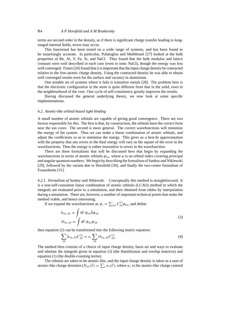
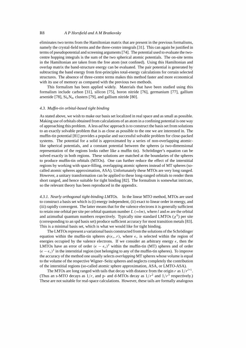
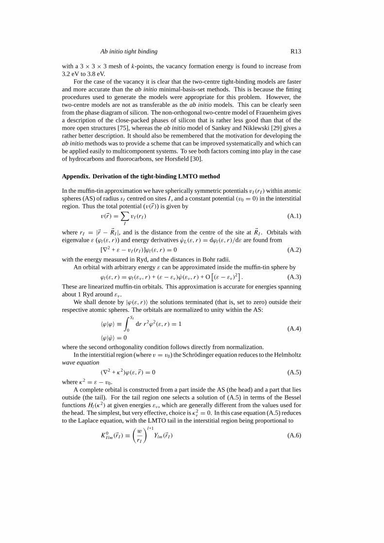
2〈V 〉). Both theseproblems can be overcome very elegantly by taking the orbitals (and also the charge density)from a confined atom. This puts the atom into a slightly excited state. In the method of Sankeyand Niklewski the atom is confined by forcing the orbitals (but not their derivatives) to go tozero at some radius (5 Bohr radii for silicon). This is equivalent to confining the atoms in aninfinitely deep spherical square well potential (see figure 1).

0 2 4r (Bohr radii)

0.00

0.05

0.10

0.15

Ψ

s orbital

0 2 4 6r (Bohr radii)

p orbital

Figure 1. A comparison of two sets of orbitals for a minimal basis set for silicon. The full linescorrespond to the orbitals used by Sankey and Niklewski, and the broken line to those used byHorsfield. The qualities of the basis sets are essentially the same. However, the basis set of Sankeyand Niklewski has a discontinuity in its first derivative at the cut-off radius.

The overlap integrals (OIα,Jβ =∫

dEr φIαφJβ) and kinetic energy integrals (TIα,Jβ =∫dEr φIαT φJβ) clearly consist of one-centre (I = J ) and two-centre (I 6= J ) terms.

The electrostatic part of the double counting (− 12

∑IJ

∫dEr dEr ′ nI (Er)nJ (Er ′)/|Er − Er ′| +

12

∑I 6=J ZIZJ /| ERI − ERJ |) also consists of one- and two-centre terms.The Hartree potential and the local part of the atomic pseudopotential can be combined

to form a short-ranged neutral-atom potential

v(NA)(Er) =∑I

{vI (Er) +

∫dEr ′ nI (

Er ′)|Er − Er ′|

}=∑I

v(NA)I (Er). (5)


A typical matrix element involving this potential is∫dEr φIα(Er)v(NA)(Er)φJβ(Er) =

∑K

∫dEr φIα(Er)v(NA)K (Er)φJβ(Er). (6)

If I = J = K we have a one-centre integral. IfI 6= J , butK = I orK = J , then we have atwo-centre integral. Otherwise we have a three-centre integral.

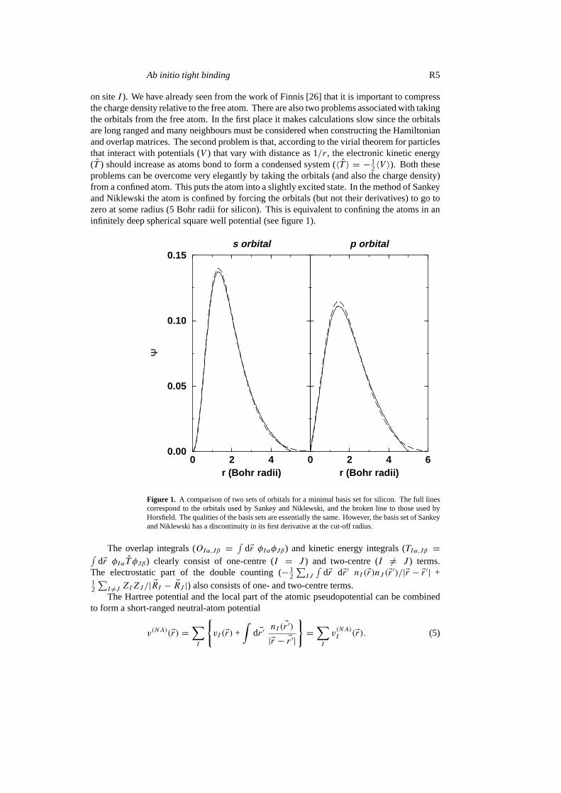
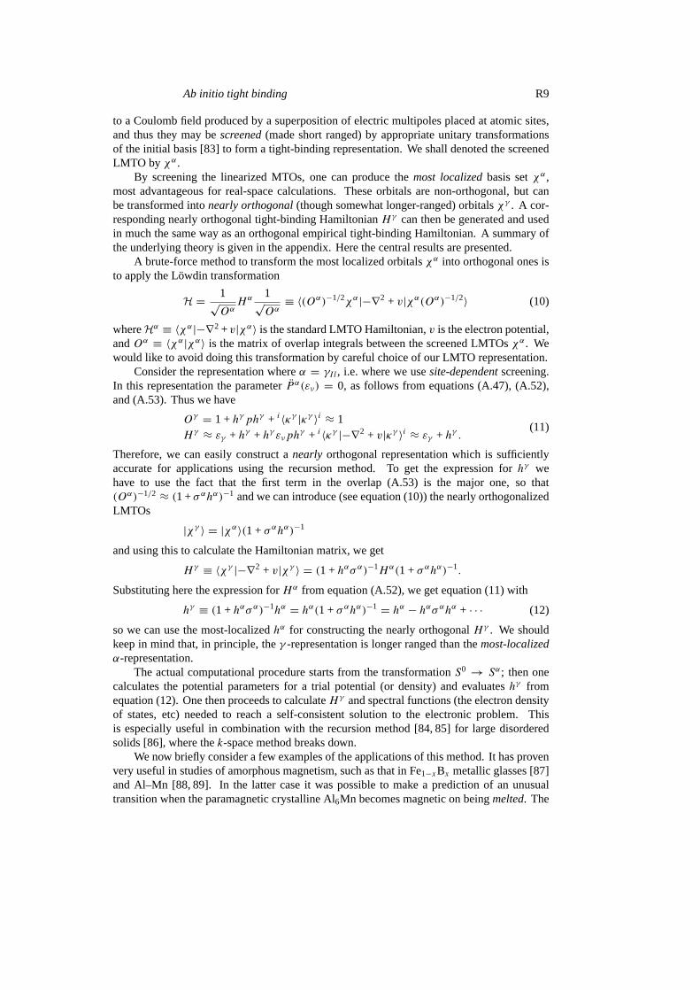
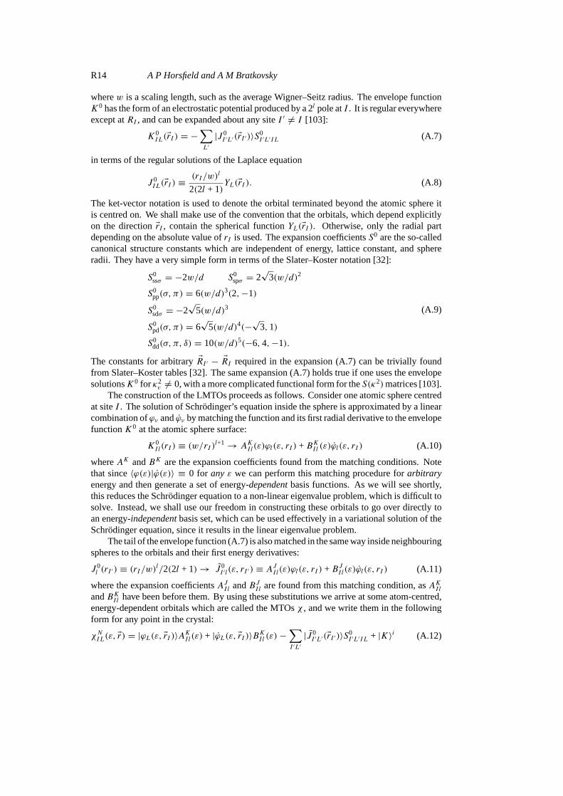
The one-centre integrals can be evaluated once and stored. The two-centre integrals canbe tabulated as a function of separation on a one-dimensional grid, with rotations being takeninto account by means of Slater–Koster [32] tables. The three-centre integrals are tabulatedas a function of three variables (see figure 2): the bond length (r), the distance between thebond centre and the site on which the potential appears (s), and an angle (θ ). The tables arecreated for a specific geometry, and the integrals for other geometries are obtained by meansof rotations. The integrals are three dimensional, and are performed in reciprocal space as thisallows two out of the three integrals to be performed analytically, leaving a one-dimensionalintegral to be performed numerically.

θ sr

z

x

a)

z

x

r

s

θ

b)

Figure 2. The geometry used to define variables in terms of which the three-centre tables areconstructed. Panel (a) is for the method of Sankey and Niklewski, and panel (b) is for the methodof Horsfield.

The electrostatic integrals are easy to tabulate because the total potential can be expressedas a linear combination of spherical single-site quantities. However, the integrals involving theexchange and correlation potential and energy are more difficult to handle because the functionsinvolved have a strongly sub-linear dependence on density (roughlyn1/3). In the Sankey–Niklewski method this functional dependence is exploited by approximating the density in someregion by an optimized constant value, for which the integrals are easy to evaluate. Considerthe integral of the exchange and correlation potential in the local density approximation∫

dEr φIα(Er)vxc(nin(Er))φJβ(Er)

≈∫

dEr φIα(Er)vxc(n)φJβ(Er) +∫

dEr φIα(Er)v′xc(n)(nin(Er)− n)φJβ(Er) + · · ·= vxc(n)OIα,Jβ + v′xc(n)(nIα,Jβ − nOIα,Jβ) + · · · (7)

wherenIα,Jβ =∫

dEr φIα(Er)nin(Er)φJβ(Er). The optimum constant value for the density (n) ischosen so as to make the second term zero (n = nIα,Jβ/OIα,Jβ). Care has to be taken whenthe overlap goes to zero. Dipole and quadrupole fluctuation corrections are included.


The method has been applied to such systems as amorphous silicon [33–39], siliconclusters [40], silicon surfaces [41, 42], various carbon structures [43–51], a number ofmulticomponent problems such as GeSe [52] and Si–C alloys [53], as well as many others[54–70].

4.2.2. Formalism of Horsfield. The formalism of Horsfield [30] is rather similar to that ofSankey and Niklewski. The important differences are the choice of basis set, and the way inwhich the exchange and correlation integrals are handled.

A minimal basis set was found to be inadequate for an accurate description of fluoro-carbons, but a double-numeric basis set gave good agreement with accurate density functionalcalculations. The orbitals were taken from the neutral atom and a positively charged ion [71].As with the formalism of Sankey and Niklewski the atomic calculations were performed in aconfining potential. The potential had the formr6. The square-well potential was not usedbecause it produces a discontinuity in the first derivative of the wavefunction at the cut-off radius(see figure 1). The integrals were all performed in real space using partition functions [71].

The perspective taken when evaluating the exchange and correlation integrals is ratherdifferent from that of Sankey and Niklewski. The key point is no longer the sub-lineardependence of the functionals on density, but rather the localized character of the confinedatomic charge densities. For the exchange and correlation potential integrals, this localizationallows us to write a many-centre expansion of the form∫

dEr φIα(Er)vxc[nin; Er]φJβ(Er)

≈∫

dEr φIα(Er)vxc[nI + nJ ; Er]φJβ(Er)

+∑

K(6=I,J )

∫dEr φIα(Er){vxc[nI + nJ + nK; Er] − vxc[nI + nJ ; Er]}φJβ(Er) + · · · .

(8)

As for the electrostatic terms we have one-, two-, and three-centre (and higher) terms. Theseare added to the electrostatic and kinetic energy terms to create a single set of tables (seefigure 2 for the geometry used for the three-centre integrals). It was found to be necessaryto carry out an additional numerical integral for the on-site exchange and correlation termsince the few-centre approximation is not accurate enough in this case. However, the integralrequires only a few points, and so is fast to evaluate. This method gives very good agreementwith accurate self-consistent calculations for molecules [30].

4.2.3. Formalism of Frauenheim.It could be argued that this is not strictly a first-principlesmethod in that it requires the fitting of a pair potential, but it does make use of tabulatedintegrals for the hopping integrals and overlap matrix, and has been used very successfully;thus it is considered here. The form used for the total energy is

UFrauenheim =∑i

fiεi +1

2

∑I 6=J

φIJ (| ERI − ERJ |) (9)

whereφIJ is a short-ranged repulsive pair potential. This form can be justified in terms ofscreening arguments [72].

As for the previous two formalisms the orbitals are obtained from atomic calculationswith the atoms being confined by a localizing potential, the form used beingr2 [73]. Oncethe orbitals are chosen, the overlap and Hamiltonian matrices can be generated. This method


eliminates two terms from the Hamiltonian matrix that are present in the previous formalisms,namely the crystal-field terms and the three-centre integrals [31]. This can again be justified interms of pseudopotential and screening arguments [74]. The potential used to evaluate the two-centre hopping integrals is the sum of the two spherical atomic potentials. The on-site termsin the Hamiltonian are taken from the free atom (not confined). Using this Hamiltonian andoverlap matrix the band-structure energy can be evaluated. The pair potential is generated bysubtracting the band energy from first-principles total-energy calculations for certain selectedstructures. The absence of three-centre terms makes this method faster and more economicalwith its use of memory as compared with the previous two methods.

This formalism has been applied widely. Materials that have been studied using thisformalism include carbon [31], silicon [75], boron nitride [76], germanium [77], galliumarsenide [78], SinNm clusters [79], and gallium nitride [80].

4.3. Muffin-tin orbital-based tight binding

As stated above, we wish to make our basis set localized in real space and as small as possible.Making use of orbitals obtained from calculations of an atom in a confining potential is one wayof approaching this problem. A lessad hocapproach is to construct the basis set from solutionsto an exactly solvable problem that is as close as possible to the one we are interested in. Themuffin-tin potential [81] provides a popular and successful solvable problem for close-packedsystems. The potential for a solid is approximated by a series of non-overlapping atomic-like spherical potentials, and a constant potential between the spheres (a two-dimensionalrepresentation of the regions looks rather like a muffin tin). Schrodinger’s equation can besolved exactly in both regions. These solutions are matched at the boundaries of the spheresto produce muffin-tin orbitals (MTOs). One can further reduce the effect of the interstitialregions by working with space-filling, overlapping atomic spheres instead of MT spheres (so-called atomic spheres approximation, ASA). Unfortunately these MTOs are very long ranged.However, a unitary transformation can be applied to these long-ranged orbitals to render themshort ranged, and hence suitable for tight binding [82]. The formalism is somewhat intricate,so the relevant theory has been reproduced in the appendix.

4.3.1. Nearly orthogonal tight-binding LMTOs.In the linear MTO method, MTOs are usedto construct a basis set which is (i) energy independent, (ii) exact to linear order in energy, and(iii) rapidly convergent. The latter means that for the valence electrons it is generally sufficientto retain one orbital per site per orbital quantum numberL (=lm), wherel andm are the orbitaland azimuthal quantum numbers respectively. Typically nine standard LMTOs (χ0) per site(corresponding to an spd basis set) produce sufficient accuracy for most transition metals [83].This is a minimal basis set, which is what we would like for tight binding.

The LMTOs represent a variational basis constructed from the solutions of the Schrodingerequation within the muffin-tin spheresφ(εν, r), whereεν is selected within the region ofenergies occupied by the valence electrons. If we consider an arbitrary energyε, then theLMTOs have an error of order(ε − εν)2 within the muffin-tin (MT) spheres and of order(ε− εν)1 in the interstitial region (not belonging to any of the muffin-tin spheres). To improvethe accuracy of the method one usually selectsoverlappingMT spheres whose volume is equalto the volume of the respective Wigner–Seitz spheres and neglects completely the contributionof the interstitial regions (so-called atomic sphere approximation, ASA, or LMTO-ASA).

The MTOs are long ranged with tails that decay with distance from the originr as 1/rl+1.(Thus an s-MTO decays as 1/r, and p- and d-MTOs decay as 1/r2 and 1/r3 respectively.)These are not suitable for real-space calculations. However, these tails are formally analogous


to a Coulomb field produced by a superposition of electric multipoles placed at atomic sites,and thus they may bescreened(made short ranged) by appropriate unitary transformationsof the initial basis [83] to form a tight-binding representation. We shall denoted the screenedLMTO by χα.

By screening the linearized MTOs, one can produce themost localizedbasis setχα,most advantageous for real-space calculations. These orbitals are non-orthogonal, but canbe transformed intonearly orthogonal(though somewhat longer-ranged) orbitalsχγ . A cor-responding nearly orthogonal tight-binding HamiltonianHγ can then be generated and usedin much the same way as an orthogonal empirical tight-binding Hamiltonian. A summary ofthe underlying theory is given in the appendix. Here the central results are presented.

A brute-force method to transform the most localized orbitalsχα into orthogonal ones isto apply the Lowdin transformation

H = 1√Oα

Hα 1√Oα≡ 〈(Oα)−1/2χα|−∇2 + v|χα(Oα)−1/2〉 (10)

whereHα ≡ 〈χα|−∇2 +v|χα〉 is the standard LMTO Hamiltonian,v is the electron potential,andOα ≡ 〈χα|χα〉 is the matrix of overlap integrals between the screened LMTOsχα. Wewould like to avoid doing this transformation by careful choice of our LMTO representation.

Consider the representation whereα = γIl , i.e. where we usesite-dependentscreening.In this representation the parameterP α(εν) = 0, as follows from equations (A.47), (A.52),and (A.53). Thus we have

Oγ = 1 +hγ phγ + i〈κγ |κγ 〉i ≈ 1Hγ ≈ εγ + hγ + hγ ενph

γ + i〈κγ |−∇2 + v|κγ 〉i ≈ εγ + hγ .(11)

Therefore, we can easily construct anearly orthogonal representation which is sufficientlyaccurate for applications using the recursion method. To get the expression forhγ wehave to use the fact that the first term in the overlap (A.53) is the major one, so that(Oα)−1/2 ≈ (1 +σαhα)−1 and we can introduce (see equation (10)) the nearly orthogonalizedLMTOs

|χγ 〉 = |χα〉(1 +σαhα)−1

and using this to calculate the Hamiltonian matrix, we get

Hγ ≡ 〈χγ |−∇2 + v|χγ 〉 = (1 +hασα)−1Hα(1 +σαhα)−1.

Substituting here the expression forHα from equation (A.52), we get equation (11) with

hγ ≡ (1 +hασα)−1hα = hα(1 +σαhα)−1 = hα − hασαhα + · · · (12)

so we can use the most-localizedhα for constructing the nearly orthogonalHγ . We shouldkeep in mind that, in principle, theγ -representation is longer ranged than themost-localizedα-representation.

The actual computational procedure starts from the transformationS0 → Sα; then onecalculates the potential parameters for a trial potential (or density) and evaluateshγ fromequation (12). One then proceeds to calculateHγ and spectral functions (the electron densityof states, etc) needed to reach a self-consistent solution to the electronic problem. Thisis especially useful in combination with the recursion method [84, 85] for large disorderedsolids [86], where thek-space method breaks down.

We now briefly consider a few examples of the applications of this method. It has provenvery useful in studies of amorphous magnetism, such as that in Fe1−xBx metallic glasses [87]and Al–Mn [88, 89]. In the latter case it was possible to make a prediction of an unusualtransition when the paramagnetic crystalline Al6Mn becomes magnetic on beingmelted. The


real-space recursion TB-LMTO method was extended to treat arbitrarynon-collinearmagneticstructures (i.e. with arbitrary directions of the exchange potential1

2E1I Eσ , whereEσ are the Pauli

matrices) which made it possible to establish the existence of a random magnetic order in Al–Mn liquids in [89], and investigate complex magnetism and magnetization direction switchingin ultrathin Co/Cu films [90,91]. In the latter case the convergence was achieved to better than0.0004 electrons au−3 for electron densities and about 0.003◦ for spin directions. The numberof iterations necessary for such a self-consistency was very large, about 1000. Additionalexamples are mentioned in e.g. [106,108].

4.3.2. Effective-medium-theory-based tight binding.In this model the total energy is givenby [92]

UEMTB =∑I

ec(sI ) +

[Eas −

∑I

eas(sI )

]+

[E1el −

∑I

e1el(sI )

]. (13)

A central quantity in this expression issI , which is the neutral-atom radius. This is the radiusof the smallest sphere centred on siteI which is charge neutral. The functionec(sI ) gives theenergy per atom in a reference system (the diamond structure for the case of silicon) with thesame neutral-atom radius. This is the large term in the expression. The following two pairs ofterms are corrections to this term which take into account the details of the environment. Thepair of terms (the atomic sphere terms)

[Eas −

∑I eas(sI )

]is the difference in a combined

electrostatic and exchange and correlation term between the real system (Eas) and the referencesystem. The term for the real system is expressed as a density-dependent pair potential. Thefinal pair of terms is the difference in the one-electron energies between the real system and thereference system. A two-centre TB-LMTO Hamiltonian is used to evaluate the one-electronenergies for the real system. This method has been applied to a number of problems involvingsilicon [93–95].

5. Introducing self-consistency

One of the main limitations of the formalisms described above is the absence of charge self-consistency. This is important for many systems, and so a number of attempts have been madeto include self-consistency into the tight-binding models. The schemes range from simplemonopolar corrections to full self-consistency with no shape approximations for the chargedensity.

Elstneret al [96] introduced self-consistency into the formalism of Frauenheim. We beginwith this approach because it can be applied to any tight-binding formalism (empirical as wellasab initio). Self-consistency is introduced by means of the addition of the following term tothe tight-binding expression for the total energy:

1E = 1

2

∑I,J

qI qJ γI,J (14)

whereγI,J =∫

dEr dEr ′ FI (|Er − ERI |)FJ (|Er ′ − ERJ |)/|Er − Er ′|. The functionFI (r) is a sphericalcharge density, normalized to 1, and is taken to have an exponential form. Gaussians couldalso be used, as they make the algebra simpler [97]. The chargesqI are given by Mullikenpopulation analysis (qI =

∑α,Jβ,i C

(i)IαfiC

(i)JβOJβ,Iα − ZI ). Minimizing the total energy with

respect to the expansion coefficientsC(i)Iα gives the self-consistent Hamiltonian

hIα,Jβ = h(0)Iα,Jβ +1

2(wI +wJ )OIα,Jβ (15)


where h(0)Iα,Jβ is the non-self-consistent Hamiltonian, and where the energy shiftwI =∑J qJ γI,J . The force on an atom is given by

EFK = EF (0)K −∑Iα,Jβ,i

C(i)IαfiC

(i)Jβ

(wI +wJ )

2

∂OIα,Jβ

∂ ERK− 1

2

∑I,J

qI qJ∂γI,J

∂ ERK(16)

where EF (0)K is the force evaluated using the expression for non-self-consistent tight binding.Formally this expression ignores any contribution from exchange and correlation.

However, the main contribution to self-consistency is from the on-site term, and the decayrates of the functionsFI are adjusted to give an on-site value (γI,I ) that agrees with eitherexperiment or first-principles calculations, and thus includes correlation.

There have been two attempts to include self-consistency into the formalism of Sankeyand Niklewski within the spherical charge approximation [55,61]. Here we will only considerthe later method [61]. Consider silicon. It has s and p valence electrons. Self-consistency isachieved by varying the number of s and p electrons contributing to the charge density on eachsite. This allows both for promotion of electrons from s to p, and for the net accumulation ofcharge. The number of s and p electrons is determined from the output wavefunctions usingthe projection onto the Lowdin orbitals [98]. All the integrations are carried out exactly asbefore, with one exception. When there is a net charge on a site there will be a long-rangedelectrostatic field. Integrals involving this field are treated within a dipole approximation.

The formalism of Horsfield also includes approximate self-consistency. It assumesspherical input charges, but allows them to vary asnI (Er) = n

(0)I (Er) + qI1I (Er), wheren(0)I

is the charge density from the neutral atom. The perturbing charge density1I is spherical,normalized to one, and constructed from partially occupied orbitals. The Hamiltonianmatrix elements are assumed to vary linearly withqI , and the double-counting term to varyquadratically. For the electrostatic terms this is the correct behaviour, but for the exchange andcorrelation terms this is approximate. The long-ranged electrostatic fields are handled usinga low-order Gaussian expansion for the orbitals which allows analytic expressions to be used.The values ofqI are found by maximizing the total energy. This follows from the fact that theHarris–Foulkes functional is maximized by the correct input charge density [99] (unlike theKohn–Sham functional which is minimized).

The formalism of Lin and Harris [99] is self-consistent from the beginning. The maindifference as compared with the tight-binding formalisms described above is that analyticfunctions are used for the orbitals and input charge density, allowing all the integrals exceptthose involving exchange and correlation to be expressed in closed form. A quadratic approx-imation is made for the exchange and correlation energy. The charge on each site is found bymaximizing the total energy.

All the above self-consistent schemes make the approximation that the input chargedensity is a sum of atom-centred spherical charge densities. Ordejonet al [100] relaxedthis approximation and represent the difference between the sum of atomic densities and theself-consistent density on a uniform mesh. They thus turned the formalism of Sankey andNiklewski into a fully self-consistent LCAO method.

6. Comparison of methods

In order to give some idea of the relative efficiencies and accuracies of the methods describedabove, calculations of the formation energy of the relaxed isolated vacancy in silicon wereperformed. All the calculations use a 64-atom cell with one atom removed. Only the0

point is used for sampling the Brillouin zone. The basis set is always minimal (s and p).


The calculations were performed using the program Plato (package for linear combination ofatomic-type orbitals).

The times we consider are for the evaluation of one total energy and set of atomic forces,and we will measure them relative to the time for non-self-consistent orthogonal empirical tightbinding. The methods considered are: empirical orthogonal tight binding using the parametersof Bowler et al [101]; the non-orthogonal tight binding of Frauenheim; theab initio tightbinding of Horsfield; and full linear combination of atomic orbitals (LCAO) with many ofthe integrals evaluated during the calculation. With the exception of the full LCAO method,self-consistency is imposed using the monopole method of Elstneret al [96]. From table 1 wecan draw several general conclusions.

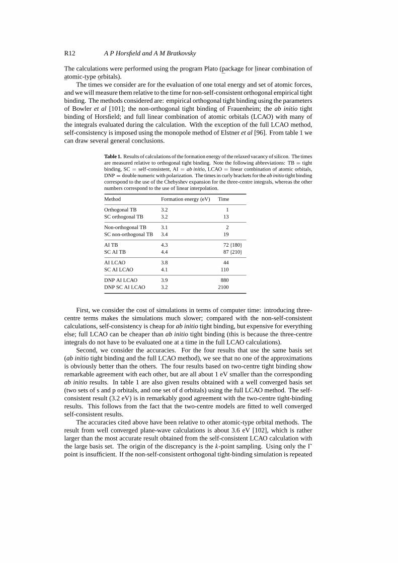
Table 1. Results of calculations of the formation energy of the relaxed vacancy of silicon. The timesare measured relative to orthogonal tight binding. Note the following abbreviations: TB= tightbinding, SC= self-consistent, AI= ab initio, LCAO = linear combination of atomic orbitals,DNP= double numeric with polarization. The times in curly brackets for theab initio tight bindingcorrespond to the use of the Chebyshev expansion for the three-centre integrals, whereas the othernumbers correspond to the use of linear interpolation.

Method Formation energy (eV) Time

Orthogonal TB 3.2 1SC orthogonal TB 3.2 13

Non-orthogonal TB 3.1 2SC non-orthogonal TB 3.4 19

AI TB 4.3 72{180}SC AI TB 4.4 87{210}AI LCAO 3.8 44SC AI LCAO 4.1 110

DNP AI LCAO 3.9 880DNP SC AI LCAO 3.2 2100

First, we consider the cost of simulations in terms of computer time: introducing three-centre terms makes the simulations much slower; compared with the non-self-consistentcalculations, self-consistency is cheap forab initio tight binding, but expensive for everythingelse; full LCAO can be cheaper thanab initio tight binding (this is because the three-centreintegrals do not have to be evaluated one at a time in the full LCAO calculations).

Second, we consider the accuracies. For the four results that use the same basis set(ab initio tight binding and the full LCAO method), we see that no one of the approximationsis obviously better than the others. The four results based on two-centre tight binding showremarkable agreement with each other, but are all about 1 eV smaller than the correspondingab initio results. In table 1 are also given results obtained with a well converged basis set(two sets of s and p orbitals, and one set of d orbitals) using the full LCAO method. The self-consistent result (3.2 eV) is in remarkably good agreement with the two-centre tight-bindingresults. This follows from the fact that the two-centre models are fitted to well convergedself-consistent results.

The accuracies cited above have been relative to other atomic-type orbital methods. Theresult from well converged plane-wave calculations is about 3.6 eV [102], which is ratherlarger than the most accurate result obtained from the self-consistent LCAO calculation withthe large basis set. The origin of the discrepancy is thek-point sampling. Using only the0point is insufficient. If the non-self-consistent orthogonal tight-binding simulation is repeated


with a 3× 3× 3 mesh ofk-points, the vacancy formation energy is found to increase from3.2 eV to 3.8 eV.

For the case of the vacancy it is clear that the two-centre tight-binding models are fasterand more accurate than theab initio minimal-basis-set methods. This is because the fittingprocedures used to generate the models were appropriate for this problem. However, thetwo-centre models are not as transferable as theab initio models. This can be clearly seenfrom the phase diagram of silicon. The non-orthogonal two-centre model of Frauenheim givesa description of the close-packed phases of silicon that is rather less good than that of themore open structures [75], whereas theab initio model of Sankey and Niklewski [29] gives arather better description. It should also be remembered that the motivation for developing theab initio methods was to provide a scheme that can be improved systematically and which canbe applied easily to multicomponent systems. To see both factors coming into play in the caseof hydrocarbons and fluorocarbons, see Horsfield [30].

Appendix. Derivation of the tight-binding LMTO method

In the muffin-tin approximation we have spherically symmetric potentialsvI (rI )within atomicspheres (AS) of radiussI centred on sitesI , and a constant potential(v0 = 0) in the interstitialregion. Thus the total potential (v(Er)) is given by

v(Er) =∑I

vI (rI ) (A.1)

whererI = |Er − ERI |, and is the distance from the centre of the site atERI . Orbitals witheigenvalueε (ϕl(ε, r)) and energy derivatives ˙ϕL(ε, r) = dϕl(ε, r)/dε are found from

[∇2 + ε − vI (rI )]ϕl(ε, r) = 0 (A.2)

with the energy measured in Ryd, and the distances in Bohr radii.An orbital with arbitrary energyε can be approximated inside the muffin-tin sphere by

ϕl(ε, r) = ϕl(εν, r) + (ε − εν)ϕ(εν, r) + O[(ε − εν)2

]. (A.3)

These are linearized muffin-tin orbitals. This approximation is accurate for energies spanningabout 1 Ryd aroundεν .

We shall denote by|ϕ(ε, r)〉 the solutions terminated (that is, set to zero) outside theirrespective atomic spheres. The orbitals are normalized to unity within the AS:

〈ϕ|ϕ〉 ≡∫ SI

0dr r2ϕ2(ε, r) = 1

〈ϕ|ϕ〉 = 0

(A.4)

where the second orthogonality condition follows directly from normalization.In the interstitial region (wherev = v0) the Schrodinger equation reduces to the Helmholtz

wave equation

(∇2 + κ2)ϕ(ε, Er) = 0 (A.5)

whereκ2 = ε − v0.A complete orbital is constructed from a part inside the AS (the head) and a part that lies

outside (the tail). For the tail region one selects a solution of (A.5) in terms of the BesselfunctionsHl(κ2) at given energiesεν , which are generally different from the values used forthe head. The simplest, but very effective, choice isκ2

ν = 0. In this case equation (A.5) reducesto the Laplace equation, with the LMTO tail in the interstitial region being proportional to

K0I lm(ErI ) ≡

(w

rI

)l+1

Ylm(ErI ) (A.6)


wherew is a scaling length, such as the average Wigner–Seitz radius. The envelope functionK0 has the form of an electrostatic potential produced by a 2l pole atI . It is regular everywhereexcept atRI , and can be expanded about any siteI ′ 6= I [103]:

K0IL(ErI ) = −

∑L′|J 0I ′L′(ErI ′)〉S0

I ′L′IL (A.7)

in terms of the regular solutions of the Laplace equation

J 0IL(ErI ) ≡

(rI /w)l

2(2l + 1)YL(ErI ). (A.8)

The ket-vector notation is used to denote the orbital terminated beyond the atomic sphere itis centred on. We shall make use of the convention that the orbitals, which depend explicitlyon the directionErI , contain the spherical functionYL(ErI ). Otherwise, only the radial partdepending on the absolute value ofrI is used. The expansion coefficientsS0 are the so-calledcanonical structure constants which are independent of energy, lattice constant, and sphereradii. They have a very simple form in terms of the Slater–Koster notation [32]:

S0ssσ = −2w/d S0

spσ = 2√

3(w/d)2

S0pp(σ, π) = 6(w/d)3(2,−1)

S0sdσ = −2

√5(w/d)3

S0pd(σ, π) = 6

√5(w/d)4(−

√3, 1)

S0dd(σ, π, δ) = 10(w/d)5(−6, 4,−1).

(A.9)

The constants for arbitraryERI ′ − ERI required in the expansion (A.7) can be trivially foundfrom Slater–Koster tables [32]. The same expansion (A.7) holds true if one uses the envelopesolutionsK0 for κ2

ν 6= 0, with a more complicated functional form for theS(κ2)matrices [103].The construction of the LMTOs proceeds as follows. Consider one atomic sphere centred

at siteI . The solution of Schrodinger’s equation inside the sphere is approximated by a linearcombination ofϕν andϕν by matching the function and its first radial derivative to the envelopefunctionK0 at the atomic sphere surface:

K0I l(rI ) ≡ (w/rI )l+1→ AKIl(ε)ϕl(ε, rI ) +BKIl (ε)ϕl(ε, rI ) (A.10)

whereAK andBK are the expansion coefficients found from the matching conditions. Notethat since〈ϕ(ε)|ϕ(ε)〉 ≡ 0 for any ε we can perform this matching procedure forarbitraryenergy and then generate a set of energy-dependentbasis functions. As we will see shortly,this reduces the Schrodinger equation to a non-linear eigenvalue problem, which is difficult tosolve. Instead, we shall use our freedom in constructing these orbitals to go over directly toan energy-independentbasis set, which can be used effectively in a variational solution of theSchrodinger equation, since it results in the linear eigenvalue problem.

The tail of the envelope function (A.7) is also matched in the same way inside neighbouringspheres to the orbitals and their first energy derivatives:

J 0l (rI ′) ≡ (rI /w)l/2(2l + 1)→ J 0

I ′l(ε, rI ′) ≡ AJIl(ε)ϕl(ε, rI ) +BJIl(ε)ϕl(ε, rI ) (A.11)

where the expansion coefficientsAJIl andBJIl are found from this matching condition, asAKIlandBKIl have been before them. By using these substitutions we arrive at some atom-centred,energy-dependent orbitals which are called the MTOsχ , and we write them in the followingform for any point in the crystal:

χNIL(ε, Er) = |ϕL(ε, ErI )〉AKIl(ε) + |ϕL(ε, ErI )〉BKIl (ε)−∑I ′L′|J 0I ′L′(ErI ′)〉S0

I ′L′IL + |K〉i (A.12)


where all| 〉s are non-zeroonly in their respective atomic spheres,| 〉i is non-zero only in theinterstitial region, andNν is the normalization coefficient. It is more convenient to write MTOsin a slightly different, though equivalent, fashion. Namely, instead ofϕ andϕ one can useϕandJ 0 to arrive at a more frequently used representation of the energy-dependent MTOs:

χNIL(ε, Er) = |ϕL(ε, ErI )〉N0I l(ε) + |J 0

L(ε, ErI )〉P 0I l(ε)−

∑I ′L′|J 0I ′L′(ε, ErI ′)〉S0

I ′L′IL + |K〉i (A.13)

whereP 0I l(ε) = BKIl (ε)/BJIl(ε), N0

I l(ε) = AKIl(ε)−P 0I l(ε)A

KIl(ε). Omitting the site and orbital

indices and summation over repeating indices, one can rewrite MTOs in the compact form

χN(ε) = |ϕ(ε)〉N(ε) + |J 0(ε)〉[P 0(ε)− S0] + |K〉i (A.14)

whereN(ε) andP 0(ε) are the so-calledpotential parameterswhich are diagonal with respectto combined site and orbital indexIL. SinceχIL(ε, Er) = χIL(ε, Er − ERI ), we can use thestandard construction for the Bloch wave in a perfect crystal. Since the normalization factoris a constant we can work with

χ(ε) ≡ χNIL(ε)/NIL(εν). (A.15)

We can write a general electron wavefunction as

ψi(ε) =∑IL

C(i)ILχIL(ε). (A.16)

One is free to select the coefficientsC(i)IL such that the second term in equation (A.14) vanishes:∑I ′L′

C(i)I ′L′(ε)[P

0I ′l′(ε)δI ′L′IL − S0

I ′L′IL] = 0. (A.17)

Then the remaining part, which is a linear combination of|ϕ(ε)〉 and |K〉i , satisfies theSchrodinger equation for the muffin-tin potentialexactly. Thus, we have recovered the famousKKR tail-cancellation condition. This equation, which defines the electron energy bands,is very inconvenient indeed, since it is a non-linear equation for the eigenvaluesε. Insteadof solving this equation, we would like to construct from MTOs the most compact energy-independentbasis to use for thevariational solution of the Schrodinger equation. Moreover,we can use our flexibility in choosing energy-independent linear MTOsχ (LMTOs) to makethem accurate to first order in(ε − εν) inclusive, so that the errors will be proportional to(ε−εν)2 insidethe atomic spheres. As we mentioned earlier, our approximations mean that inthe interstitial region the error of the LMTO is proportional to(ε− εν)1, but this contributionis neglected in the atomic sphere approximation, where one selectsspace-fillingoverlappingMT spheres. We need to analyse MTOs in detail to see all this.

The matching conditions at the atomic sphere boundaries give us a two-by-two linearsystem of equations, and it is convenient to write their solutions in the following form:

P 0(ε) = W [ϕ(ε),K0]

W [ϕ(ε), J 0]= 2(2l + 1)

(w

s

)2l+1D(ε) + l + 1

D(ε)− 1(A.18)

N0(ε) = W [K0, J 0]

W [ϕ(ε), J 0]= w/2

W [ϕ(ε), J 0]=[w

2P 0(ε)

]1/2(A.19)

whereD(ε) ≡ sϕ′(ε, s)/ϕ(ε, s) is the logarithmic derivative of the wave function at theatomic sphere surface, which is simply related to the usual scattering phase shiftδl [104], andW [f1, f2] ≡ s2[f ′1(s)f2(s) − f1(s)f

′2(s)] is the Wronskian. In both cases the prime stands

for differentiation with respect to the radial variable. To derive (A.19) forN via P one shoulddifferentiate the Wronskian relation (A.18) and use

W [ϕ, ϕ] = s2(ϕϕ′ − ϕ′ϕ)r=s =∫ s

0dr r2ϕ2 = 1. (A.20)


The latter relation follows from the Schrodinger equation (A.2) and its first derivative withrespect to energy

(−∇2 + v − ε)ϕ = ϕ.It is important to note that when the tail-cancellation condition (A.17) is obeyed, the

contributions ofJ 0(ε) cancel outin the atomic sphere at the origin exactly, at least for loworbital angular momental. However, if one were to use the MTOsχ(ε) with a variationalmethod, these unwanted contributions, generally varying linearly with the energyε, wouldremain and reduce the precision of the band calculations. The energy dependence ofJ 0(ε) isobviously weak, since it matches continuously to energy-independent envelope functionK0,and can be eliminated completely to first order when using fixed energy orbitals. At any givenenergyε = ενI l in a region of interest we select the head

χhead≡ |ϕ(ε)〉 N(ε)N(εν)

+ |J 0(ε)〉P0(ε)

N(εν)

(the part of the MTO in its own atomic sphere) and chooseJ 0(εν) from the conditionχhead(εν) = 0 which gives us a condition forJ 0(εν):

|ϕ(εν)〉 + |ϕ(εν)〉 N(εν)N(εν)

+ |J 0(εν)〉 P0(εν)

N(εν)= 0. (A.21)

This relation has a pureL-character since the matrices of potential parameters are diagonalmatrices with respect to site and orbital indices. Thus, we arrive at the following substitution:

J 0(εν, r)→− ϕ(εν) + ϕ(εν)N0(εν)/N0(εν)

P 0(εν)/N0(εν)≡ −ϕ0(r)

(2

wP 0

)−1/2

(A.22)

where we have used (A.19) and introducedthe definitions

ϕ0(r) ≡ ϕ(r) + ϕ(r)σ 0 (A.23)

σ 0 ≡ N0/N0 = P 0/(2P 0) (A.24)

where we imply that all quantities without arguments are evaluated atε = εν.After we performthe substitution (A.22) in the headand the tailsof the MTO we obtain the energy-independentbasisχ(εν), which is accurate to terms O(ε − εν)2.

Substituting (A.22) in the equation (A.15), and using (A.19) we finally arrive at the workingexpression for the standard linear muffin-tin orbital (we mark this representation byzeroasthe superscript):

χ0 ≡ |ϕ〉 + |J 0〉(P 0 − S0)/N0 + |K0〉i/N0

= |ϕ〉 − |ϕ0〉(P 0)−1/2(P 0 − S0)(P 0)−1/2 + |K0〉i/N0

= |ϕ〉 + |ϕ0〉h0 + |K0〉i(

2

wP 0

)−1/2

. (A.25)

Here we have introduced the two-centrefirst-order Hamiltonian

h0 = −(P 0)−1/2(P 0 − S0)(P 0)−1/2

and have used (A.19). One can now use the constructed LMTOs to solve the Schrodingerequation by minimizing〈ψi |H − E(i)|ψi〉 with ψi taken from equation (A.16). This leads tothe standard linear problem∑

I ′L′C(i)I ′L′(HI ′L′IL − E(i)OI ′L′IL) = 0


where the matrix elements are

H ≡ 〈χ0|−∇2 + v|χ0〉= h0 + h0σ 0h0 + (1 +h0σ 0)εν(σ

0h0 + 1) + h0ενph0 + i〈κ|−∇2 + v|κ〉i

(A.26)

O ≡ 〈χ0|χ0〉 = (1 +h0σ 0)(σ 0h0 + 1) + h0ph0 + i〈κ|κ〉i (A.27)

where we have introduced an extra potential parameter

pIl = 〈(ϕI l)2〉 = −ϕl(sI )/3ϕl(sI )and

|κ〉i ≡ |K0〉i(

2

wP 0

)−1/2

.

The last terms in (A.26) and (A.27) are the so-called combined corrections. Recalling that|κ〉iis a solution of the Schrodinger equation atε = κ2 we see thati〈κ|−∇2 +v|κ〉i = κ2(i〈κ|κ〉i ).With the use of Green’s theorem and the definition of|κ〉i we can express these integrals in termsof the canonical structure constantsS0 and their first energy derivativesS ≡ ∂S/∂κ2 [105,106].Therefore, all one needs to know in order to solve the Schrodinger equation for a crystal isthe values of the partial wavefunctions and their derivatives with respect to the coordinate andenergy at the atomic sphere surface at the energyεν in the window of interest. These values areeasily found from radial solutions of the Schrodinger equation for the muffin-tin potentials.

Let us now discuss in more detail the first-order Hamiltonianh0:

h0 = −|ϕ0〉(P 0)−1/2(P 0 − S0)(P 0)−1/2 = c0 − εν +√d0S0√d0 (A.28)

where

√d0 ≡ (P 0)−1/2 =

(2

w

)1/2

W [ϕ, J 0] =(s

2

)1/2(s

w

)l+1/2

ϕ(s)l −D2l + 1

c0 − εν ≡ −P 0/P 0 = − 2

wW [ϕ,K0]W [ϕ, J 0] = sϕ2(s)

(D + l + 1)(l −D)2l + 1

whereD ≡ D[ϕν(r)] ≡ ∂ ln ϕν(r)/∂ ln r at r = s. Potential parametersc0 ≡ c0I lδI ′L′IL and

d0 ≡ d0I lδI ′L′IL are the diagonal matrices easily found from the preceding equations.

It is instructive to relate the potential parametersc0 andd0 to the scattering characteristicsof the muffin-tin potential for which they are calculated. First we recall the relation between thepotential function and the scattering phase shift, namely(P 0)−1 ∝ − tanδl . Since tanδl has aresonant character [104], it is customary to parametrize [P 0(ε)]−1 in the following functionalform:

[P 0(ε)]−1 = 1

ε − C + γ (A.29)

where thecanonical potential parametersCl (centre),1l (width), andγl of the bandl arereadily found fromϕ′(ε, s), ϕ(ε, s), and their derivatives with respect to energy.Cl is theenergy at whichD(Cl) = −l − 1. Substituting this expression into equation (A.28) we arriveat the following relations for the parameters of the first-order Hamiltonianh0:

√d0 =

√1

(1 +γ

εν − C1

)c0 − εν = (C − εν)

(1 +γ

εν − C1

).

(A.30)


If one selectsεν = C, thend0 = 1, c0 = C, and the first-order Hamiltonian becomes

h0 =√1S0√1 H ≈ H(1) ≡ εν +

√1S0√1.

Thus we have arrived at the simplest two-centre first-order Hamiltonian in real space, usefulin qualitative discussions of the band problem. For an ideal crystal one transfersH andOinto k-space by substituting for the only site-non-diagonal matrixS with its Fourier transform,calculated by the standard Ewald procedure. Since the canonical potential parametersCl ,1l ,andγl are somewhat less sensitive to a choice ofεν , one can substitute equation (A.3) intoequation (A.18) and compare with the resonant expression forP 0, equation (A.29), with thefollowing results suitable for practical calculations:

C − εν = −W [ϕ,K0]

W [ϕ, K0]= −ϕ(s)

ϕ(s)

D[ϕ(s)] + l + 1

D[ϕ(s)] + l + 1√1 =

√w/2

|W [ϕ, K0]| =1√2

(s/w)l+1/2

√s|ϕ(s)|

1

|D[ϕ(s)] + l + 1|

γ ≡ 1

P [ϕ(s)]= W [ϕ, J 0]

W [ϕ, K0]= 1

2(2l + 1)

(s

w

)2l+1D[ϕ(s)] − lD[ϕ(s)] + l + 1

.

(A.31)

In order to see that the width1 has the correct dimensionality of Ryd we recall that we areworking in atomic units, wheres has the dimensionality(Ryd)−1/2 andϕ has a dimensionalityof s−3/2 = (Ryd)3/4. This completes our discussion of thestandardLMTO method.

In order to treat large systems (meaning a few hundred atoms or more) one would like tohave a localized, accurate, and minimal basis set which one can use in afully ab initio method.The standard LMTO method operates with long-range orbitals and is not suitable for thispurpose. However, the LMTOs can be made localized with the use of the information aboutthe environment of each atom [83]. To screen the long-ranged tail ofK0(ErI ) one introduces,instead ofJ 0, a functionJ α in the expansion (A.7) which includes the screening multipoleswith chargesαIl (=0 for l > lα, where usuallylα 6 2):

J αIl(rI ) ≡ J 0I l(rI )− αIlK0

I l(rI ). (A.32)

Introducing such screening charges will inevitably change the multipole field everywhere,including the vicinity of the origin, whereK0 was centred. Thus, one has to introduce newenvelope functionsKα which are defined in all space and arelinearly related toK0 everywhere.The tail expansion now reads

KαIL(ErI ) = −

∑L′J αI ′L(ErI ′)SαI ′L′IL (A.33)

where nowSα hasnon-zeroon-site elements, sinceKα 6= K0 at the origin. Let us usecompressed matrix indicesa ≡ ILwhich imply a summation over repeated indices, and markby the superscript∞ the envelope functions defined in the whole space, while the functionswithout this sign are assumed to be truncated beyond their atomic sphere of origin. Then wehave

∞Kαa ≡ K0

a′δa′a − J αa′Sαa′a = K0a′(δa′a + αa′S

αa′a)− J 0

a′Sαa′a

∞K0a ≡ K0

a′δa‘a − J 0a′S

0a′a.

(A.34)

From our earlier discussion we expect these envelope functions to be related by a unitarytransformationUa′a such that∞Kα

a = ∞K0a′Ua′a. Comparing this with equation (A.34) we

obtain a relation betweenSα andS0 by comparing the coefficients beforeK0 andJ 0 in two ofthese expansions:

Ua′a = δa′a + αa′S0a′a ≡ 1 +αS0

Sαa′a = S0a′a′′Ua′′a = S0(1 +αSα) = S0 + S0αSα.

(A.35)


Thus we have obtained a Dyson-like equation for the screened structure constants. A solutionof the Dyson equation (A.35) can be given in the following convenient form:

Sα = S0 + S0αS0 + · · · ≡ α−1(1 +αS0 + αS0αS0 + · · · − 1)

= α−1[(1− αS0)−1− 1

] = α−1(α−1− S0)−1α−1− α−1. (A.36)

Since in a regular lattice with lattice vectorsER and ET and atomic positionEτ within the unitcell,[α−1EREτ lδ EREτL, ER+ ET Eτ ′L′ − S0

EREτL, ER+ ET Eτ ′L′]−1= (1/N)

∑Ek

[α−1EREτ l − S

0EτL,Eτ ′L′(Ek)

]−1e−iEk· ET (A.37)

where by definition

S0τL,τ ′L′(

Ek) =∑ETS0EREτL, ER+ ET Eτ ′L′e

−iEk· ET (A.38)

the long-range behaviour ofSα is defined by the analytical properties of the Fourier-transformedfunctionS0(Ek), which is customarily evaluated by means of a Ewald summation. It followsfrom the form of the canonical structure constants (A.9) thatS0(Ek) is bounded from above;therefore it is possible to find sufficiently small and positiveαs for which det[α−1−S0(Ek)] 6= 0.Since there are no poles for real values ofk in equation (A.37), its Fourier transform will befalling off exponentially with distance| ER− ER′|/w. This conclusion does not, of course, dependon whether the lattice is ordered or not. As mentioned above, it should just be sufficientlyclose packed or, for open structures, packed with empty spheres so that this recipe for screeningmight work.

We now give a simple example illustrating this procedure for screening LMTOs. Considera system with only one s orbital per site [106]. The relevant structure constant isSssσ ,equation (A.9), whose lattice Fourier transform is

S(Ek) =∑ET

−2w

Te−iEk· ET ≈ −

∫d3T

�

2w

Te−iEk· ET + constant= − 6

(kw)2+ constant (A.39)

where the constant is determined from the condition that the on-site element of theS-matrix inreal space vanishes,S ER=0 = 0= (1/N)∑Ek S(Ek),� = (4π/3)w3 is the unit-cell volume, andthe Brillouin zone was approximated by a sphere with radiusk0 such that(4π/3)k3

0 = (2π)3/�.After performing the integration we obtain

S(Ek) = − 6

(kw)2+

1

αc(A.40)

whereαc = 2−5/33−2/3π2/3 = 0.32. Substituting this into (A.36) we obtain forER 6= 0

SαE0 ER = (1/N)∑ 1

α

(1

α− 1

αc+

6

(kw)2

)−1 1

αe−iEk· ER. (A.41)

Note that this expression has no poles only ifα < αc = 0.32, i.e. the screening charges cannotexceed a certain limit. In this case, if we were to extend the integration overk to infinity, wewould get

SαE0 ER = −α2c

(αc − α)22w

Re−√

6ξ(R/w) (A.42)

where we have introducedξ ≡ ααc/(αc − α). Indeed, this matrix decays exponentially inreal space. This seemingly obvious statement [83] does not actually apply to real lattices.Obviously, the decay will be strictly exponential only whenall multipole moments of the


given charge distribution areexactly zero. Note that an actual integration is cut off at theBrillouin-zone boundary, and the actual functional dependence on the distanceR/w is givenin terms of a damped oscillatory asymptotic expansion. The complicated shape of the actualBrillouin zone, however, produces strong compensation of different oscillatory terms, so theactual behaviour is close to fast exponential decay. The optimal numerical choice for close-packed structures isαs = 0.3485,αp = 0.053 03, andαd = 0.0107, and the orbitals areessentially limited to first and second neighbours [83].

A screened LMTOχα can be constructed inexactlythe same way as the standard LMTO(A.25), with the replacements of all superscripts 0→ α, and by substituting for the potentialparameterγ with γ − α in (A.29), (A.30). Indeed, the matching conditions now read

J αIl(r) ≡(rI /w)

l

2(2l + 1)− αl

(w

rI

)l+1

→ J αI l(rI ) (A.43)

K0I l(r) ≡

(w

rI

)l+1

→ ϕIl(ε, rI )NαIl(ε) + J αI l(rI )P

αIl(ε). (A.44)

We immediately have from these matching conditions

Pα(ε) = W [ϕ(ε),K0]

W [ϕ(ε), J α]= P 0(ε)

1− αP 0(ε)(A.45)

Nα(ε) = W [K0, J α]

W [ϕ(ε), J α]=[w

2P α(ε)

]1/2(A.46)

whereP 0 is from (A.18). Rewriting (A.45) in the form[Pα(ε)

]−1 = [P 0(ε)]−1− α

and substituting the resonant expansion (A.29), we arrive at[Pα(ε)

]−1 = 1

ε − C + γ − α. (A.47)

In the expression for the Hamiltonian in the screened LMTO representation below (A.54)we shall see that all potential parameters are defined byPα(ε) and its energy derivatives.Comparing (A.47) with (A.29) we see that indeed the only difference is the replacementγ → γ − α. Repeating our reasoning for the choice ofJ α, we arrive at the followingsubstitution, which makes the screened LMTO independent of energy everywhere:

J α(εν, r)→− ϕ(εν) + ϕ(εν)Nα(εν)/Nα(εν)

P α(εν)/Nα(εν)≡ −ϕα(r)

(2

wP α)−1/2

(A.48)

where

ϕα(r) ≡ ϕ(εν) + ϕ(εν)σα (A.49)

σα ≡ Nα(εν)

Nα(εν)= P α/(2P α) (A.50)

and obtain a screened LMTO (again, we want it to start from just the atomic orbital|ϕ〉, so wedivide the initial MTO (A.44) byNα(εν)):

χα ≡ |ϕ〉 + |J α〉(P α − Sα)/Nα + |Kα〉i/Nα

= |ϕ〉 − |ϕα〉(P α)−1/2(P α − Sα)(P α)−1/2 + |Kα〉i/Nα

= |ϕ〉 + |ϕα〉hα + |Kα〉i(

2

wP α)−1/2

. (A.51)


Here we have introduced the two-centrefirst-order screened Hamiltonian

hα = −(P α)−1/2(P α − Sα)(P α)−1/2.

One can now use the screened LMTOs to solve the Schrodinger equation, which leads to thestandard linear problem∑

I ′L′Cα(i)I ′L′ (H

αI ′L′IL − E(i)Oα

I ′L′IL) = 0

where the matrix elements are

Hα ≡ 〈χα|−∇2 + v|χα〉= hα(1 +σαhα) + (1 +hασα)εν(σ

αhα + 1) + hαενphα + i〈κα|−∇2 + v|κα〉i

(A.52)

Oα ≡ 〈χα|χα〉 = (1 +hασα)(σ αhα + 1) + hαphα + i〈κα|κα〉i (A.53)

where

|κα〉i ≡ |Kα〉i(

2

wP α)−1/2

.

One can gain more insight into the screened LMTOs by looking at the parametrization ofthe Hamiltonian

hα = −(P α)−1/2(P α − Sα)(P α)−1/2 = cα − εν +√dαSα√dα (A.54)

where√dα ≡ (P α)−1/2 =

(2

w

)1/2

W [ϕ, J α] =√1

[1 + (γ − α)εν − C

1

]cα − εν ≡ −Pα/P α = − 2

wW [ϕ,Kα]W [ϕ, J α] = (C − εν)

[1 + (γ − α)εν − C

1

]where we again expressed everything in terms of our primary potential parametersC, 1, andγ (equation (A.31)). Note that it differs from (A.30) merely by substitutionγ → γ − α, aswe discussed earlier; see equation (A.47).

This finalizes our construction of the tight-binding LMTO. We see that the first-orderHamiltonian (A.54) is short ranged because it contains the screenedSα-matrices. The rangeofHα (equation (A.52)) is larger, since it contains two-hop terms, likehσh. These terms maybe treated exactly or perturbatively.

Finally we offer some comments on the accuracy of the LMTO method and recentimprovements. We have used the atomic spheres approximation (ASA) by taking the energyof our basis wave functions to beκ2

ν = 0. Thus we make an error that is linear inE−Eν in ourbasis in the interstitial region, whereas inside the MT spheres the corrections are proportional to(ε − εν)2. The LMTO-ASA is a powerful tool for close-packed solids, but these inaccuraciesmake it unsuitable for calculation of forces and dynamics. Full potential LMTO has beendesigned to allow the inclusion of any non-ASA corrections and the accurate treatment of anyinterstitial region (see [107] and references therein). It is somewhat involved, making use ofmultiple-κ2

ν basis sets to describe accurately the interstitial region.It is worth mentioning that it is in principle possible to reformulate the standard LMTO

method so that (i) the error of the basis in the interstitial region is notε − εν but (ε − εν)2,(ii) the basis set is localized in space, and (iii) the full (non-spherical) charge density andpotential are expanded via the same functions as were used to construct the basis [108]. Themain idea of using solutions of the Schrodinger equation in the MT spheres as well as theinterstitial region (A.5) with matching at the MT spheres does not change. However, in order


to localize the basis one has to solve the wave equation (A.5) such that the solution has zeroYL′(rI )-projections on other non-touching spheres with radiiaI ′l′ (these spheres are analogousto hard impenetrable spheres). Such solutions always exist, they produce a complete set, andthey may be localized. One needs these functions to obey the matching conditions of thewave functions at the MT spheres, which is done by introducing so-calledkinkypartial waves.The matching conditions at the MT spheres are then reduced to algebraic form involving thekink (KKR) matrix K. The LMTO overlap matrix and the Hamiltonian matrix can then beexpressed solely in terms of the kink KKR matrix at the selected energyEν and its firstthreeenergy derivativesK, K, and

···K. This, as we have seen, extends the spatial range of the matrix

elements.

References

[1] Ashcroft N W and Mermin D 1976Solid State Physics(Tokyo: Holt-Saunders)[2] Tan K E, Bratkovsky A M, Harris R M, Horsfield A P, Nguyen-Manh D, Pettifor D G and Sutton A P 1997

Modell. Simul. Mater. Sci. Eng.5 187[3] Kohn W and Sham L J 1965Phys. Rev.140A1133[4] Sutton A P, Finnis M W, Pettifor D G and Ohta Y 1988J. Phys. C: Solid State Phys.2135[5] Goodwin L, Skinner A J and Pettifor D G 1989Europhys. Lett.9 701[6] Xu C H, Wang C Z, Chan C T and Ho K M 1992J. Phys.: Condens. Matter4 6047[7] Kwon I, Biswas R, Wang C Z, Ho K M and Soukoulis C M 1994Phys. Rev.B 497242[8] Tang M S, Wang C Z, Chan C T and Ho K M 1996Phys. Rev.B 53979[9] Allen P B, Broughton J Q and McMahan A K 1986Phys. Rev.B 34859

[10] Khan F S and Broughton J Q 1989Phys. Rev.B 393688[11] Sawada S 1990Vacuum41612[12] Mercer J L and Chou M Y 1993Phys. Rev.B 479366[13] Mercer J L and Chou M Y 1994Phys. Rev.B 498506[14] Sigalas M M and Papaconstantopoulos D A 1994Phys. Rev.B 491574[15] Cohen R E, Mehl M J and Papaconstantopoulos D A 1994Phys. Rev.B 5014 694[16] Menon M and Subbaswamy K R 1997Phys. Rev.B 559231[17] Liu F 1995Phys. Rev.B 5210 677[18] Pople J A, Santry D P and Segal G A 1965J. Chem. Phys.43S129[19] Pople J A and Segal G A 1965J. Chem. Phys.43S136[20] Pople J A and Segal G A 1966J. Chem. Phys.443289[21] Santry D P and Segal G A 1967J. Chem. Phys.47158[22] Pople J A, Beveridge D L and Dobosh P A 1967J. Chem. Phys.472026[23] Harris J 1985Phys. Rev.B 311770[24] Foulkes W M C 1987PhD ThesisUniversity of Cambridge[25] Foulkes W M C andHaydock R 1989Phys. Rev.B 3912 520[26] Finnis M W 1990J. Phys.: Condens. Matter2 331[27] Polatoglou H M and Methfessel M 1988Phys. Rev.B 3710 403[28] Chan C T, Vanderbilt D and Louie S G 1986Phys. Rev.B 332455[29] Sankey O F and Niklewski D J 1989Phys. Rev.B 403979[30] Horsfield A P 1997Phys. Rev.B 566594[31] Porezag D, Frauenheim Th, Kohler Th, Seifert G and Kaschner R 1995Phys. Rev.B 5112 947[32] Slater J C and Koster G F 1954Phys. Rev.941498[33] Drabold D A, Fedders P A, Sankey O F and Dow J D 1990Phys. Rev.B 425135[34] Drabold D A, Fedders P A, Klemm S and Sankey O F 1991Phys. Rev. Lett.672179[35] Fedders P A, Drabold D A and Klemm S 1992Phys. Rev.B 454048[36] Fedders P A, Fu Y and Drabold D A 1992Phys. Rev. Lett.681888[37] Fedders P A and Drabold D A 1993Phys. Rev.B 4713 277[38] Kilian K A, Drabold D A and Adams J B 1993Phys. Rev.B 4817 393[39] Fedders P A 1995Phys. Rev.B 521729[40] Sankey O F, Niklewski D J, Drabold D A and Dow J D 1990Phys. Rev.B 4112 750[41] Adams G B and Sankey O F 1991Phys. Rev. Lett.67867[42] Feil H, Zandvliet J W, Tsai M-H, Dow J D and Tsong I S T1992Phys. Rev. Lett.693076


[43] Adams G B, Page J B, Sankey O F, Sinha K, Menendez J and Huffman D R 1991Phys. Rev.B 444052[44] O’Keeffe M, Adams G B and Sankey O F 1992Phys. Rev. Lett.682325[45] Drabold D A, Wang R, Klemm S, Sankey O F and Dow J D 1991Phys. Rev.B 435132[46] Yang S H, Drabold D A and Adams J B 1993Phys. Rev.B 485261[47] Alfonso D R, Yang S H and Drabold D A 1994Phys. Rev.B 5015 369[48] Drabold D A, Fedders P A and Stumm P 1994Phys. Rev.B 4916 415[49] Adams G B, Page J B, Sankey O F and O’Keeffe M 1994Phys. Rev.B 5017 471[50] Alfonso D R, Drabold D A and Ulloa S E 1995Phys. Rev.B 511989[51] Alfonso D R, Drabold D A and Ulloa S E 1995Phys. Rev.B 5114 669[52] Cappelletti R L, Cobb M, Drabold D A and Kamitakahara W A 1995Phys. Rev.B 529133[53] Demkov A A and Sankey O F 1993Phys. Rev.B 482207[54] Phillips R, Drabold D A, Lenosky T, Adams G B and Sankey O F 1992Phys. Rev.B 461941[55] Tsai M-H, Sankey O F and Dow J D 1992Phys. Rev.B 4610 464[56] Yang S H, Drabold D A, Adams J B and Sachdev A 1993Phys. Rev.B 471567[57] Adams G B, O’Keeffe M, Demkov A A, Sankey O F and Huang Y-M 1994Phys. Rev.B 498048[58] Caro A, Drabold D A and Sankey O F 1994Phys. Rev.B 496647[59] Ortega J, Lewis J P and Sankey O F 1994Phys. Rev.B 5010 516[60] Demkov A A, Sankey O F, Schmidt K E, Adams G B and O’Keeffe M 1994Phys. Rev.B 5017 001[61] Demkov A A, Ortega J, Sankey O F and Grumbeth M P 1995Phys. Rev.B 521618[62] Huang Y M, Spence J C H andSankey O F 1995Phys. Rev. Lett.743392[63] Landman J I, Morgan C G and Schick J T 1995Phys. Rev. Lett.744007[64] Park Y K, Estreicher S K, Myles C W and Fedders P A 1995Phys. Rev.B 521718[65] Demkov A A, Windl W and Sankey O F 1996Phys. Rev.B 5311 288[66] Demkov A A and Sankey O F 1997Phys. Rev.B 5610 497[67] Lewis J P, Ordejon P and Sankey O F 1997Phys. Rev.B 556880[68] Demkov A A, Sankey O F, Gryko J and McMillan P F 1997Phys. Rev.B 556904[69] Fritsch J, Sankey O F and Schmidt K E 1998Phys. Rev.B 5715 360[70] Windl W, Sankey O F and Menendez J 1998Phys. Rev.B 572431[71] Delley B 1990J. Chem. Phys.92508[72] Seifert G, Porezag D and Frauenheim T 1996Int. J. Quantum Chem.58185[73] Eschrig H 1979Phys. Status Solidib 96329[74] Seifert G, Eschrig H and Bieger W 1986Z. Phys. Chem.267529[75] Frauenheim Th, Weich F, Kohler Th, Uhlmann S, Porezag D and Seifert G 1995Phys. Rev.B 5211 492[76] Widany J, Frauenheim Th, Porezag D, Kohler Th and Seifert G 1996Phys. Rev.B 534443[77] Sitch P and Frauenheim Th 1996J. Phys.: Condens. Matter8 6873[78] Haugk M, Elsner J and Frauenheim Th 1997J. Phys.: Condens. Matter9 7305[79] Jackson K A, Jungnickel G and Frauenheim Th 1998Chem. Phys. Lett.292235[80] Elsner J, Jones R, Heggie M I, Sitch P K, Haugk M, Frauenheim Th,Oberg S and Briddon P R 1998Phys.

Rev.B 5812 571[81] Ziman J 1965Principles in the Theory of Solids(Cambridge: Cambridge University Press)[82] Andersen O K 1975Phys. Rev.B 123060[83] Andersen O K, Pawlowska Z and Jepsen O 1986Phys. Rev.B 345253

Andersen O K and O Jepsen 1984Phys. Rev. Lett.532571[84] Haydock R, Heine V and Kelly M J 1975J. Phys. C: Solid State Phys.8 2591[85] Heine V, Bullett D W, Haydock R and Kelly M J 1980Solid State Physicsvol 35, ed F Seitz and D Turnbull

(New York: Academic)[86] Nowak H J, Andersen O K, Fujiwara T and Jepsen O 1991Phys. Rev.B 443577[87] Bratkovsky A M and Smirnov A V 1993Phys. Rev.B 489606[88] Bratkovsky A M, Smirnov A V, Nguyen Manh D and Pasturel A 1995Phys. Rev.B 523056[89] Smirnov A V and Bratkovsky A M 1996Phys. Rev.B 538515[90] Smirnov A V and Bratkovsky A M 1996Phys. Rev.B 54R17 371[91] Smirnov A V and Bratkovsky A M 1997Phys. Rev.B 5514 434[92] Stokbro K, Chetty N, Jacobsen K W and Norskov J K 1994Phys. Rev.B 5010 727[93] Hansen L B, Stokbro K, Lundqvist B I, Jacobsen K W and Deaven D M 1995Phys. Rev. Lett.754444[94] Stokbro K, Jacobsen K W, Norskov J K, Deaven D M, Wang C Z and Ho K M 1996Surf. Sci.360221[95] Hansen L B, Stokbro K, Lundqvist B I and Jacobsen K W 1996Mater. Sci. Eng.B 37185[96] Elstner M, Porezag D, Jungnickel G, Elsner J, Haugk M, Frauenheim Th, Suhai S and Seifert G 1998Phys.

Rev.B 587260


[97] Horsfield A P, Dunham S and Fujitani H 1998MRS Proc. (Fall 1998)(Warrendale, PA: Materials ResearchSociety) Symposium J

[98] Lowdin P 1950J. Chem. Phys.18365[99] Lin Z and Harris J 1992J. Phys.: Condens. Matter4 1055

[100] Ordejon P, Artacho E and Soler J M 1996Phys. Rev.B 53R10 431[101] Bowler D, Fearn M, Goringe C, Horsfield A and Pettifor D 1998J. Phys.: Condens. Matter103719[102] Mercer J L, Nelson J S, Wright A F and Stechel E B 1998Modell. Simul. Mater. Sci. Eng.6 1[103] Varshalovich D A, Moskalev A N and Khersonskii V K 1989 Quantum Theory of Angular Momentum

(Singapore: World Scientific)[104] Landau L D and Lifshitz E M 1977Quantum Mechanics, Non-Relativistic Theory3rd edn (Oxford: Pergamon)[105] Bratkovsky A M and Savrasov S Yu 1990J. Comput. Phys.88243[106] Andersen O K, Jepsen O and Sob M 1987Electronic Band Structure and its Applications (Springer Lecture

Notes in Physics, vol 283)ed M Yussouff (Berlin: Springer)[107] Savrasov S Yu and Savrasov D Yu 1992Phys. Rev.B 4612 181

Savrasov S Yu 1992Phys. Rev. Lett.692819Savrasov S Yu 1998Phys. Rev. Lett.812570

[108] Andersen O K, Jepsen O and Krier G 1994PreprintAndersen O K, Arcangeli C, Tank R W, Saha-Dasgupta T, Krier G, Jepsen O and Dasgupta I 1998Proc. Mater.

Res. Soc.vol 491 (Warrendale, PA: Materials Research Society) p 3

Documents

Ab initio tight binding