Ab initio molecular dynamics : BO

Vardha SrinivasanIISER Bhopal

School on First Principles Simulations, JNCASR, 2010

Why ab initio MD

• Free of parametrization and only fundamental constants required.

• Bond forming and breaking processes can be treated accurately.

• Transferable unlike many classical MD methods.

• “On the fly” computation of potential energy surface, so avoids dimensionality bottleneck.

Quantum dynamics

r electrons R (RI) ions

H = − �22MI

∇I2 − �2

2me∇e

2 + Ve−e + VI−I + Ve−I

electron-electron repulsion

ion-ion repulsion

electron-ion attraction

i� ∂

∂tΨ(r,R; t) = HΨ(r,R; t)

Complicated Full quantum dynamics quite messy and not needed in most cases.

Ψ(r,R; t)

Decoupling electrons and ions

He = − �22me

∇2e + Ve−e + VI−I + Ve−I

Heψk(r;R) = Ek(R)ψk(r;R)

First solve for clamped nuclei

Instantaneous representation for full solution

Integrate out r dependence

Ψ(r,R; t) =�

l

ψl(r;R)χl(R; t)

�dr ψk(r;R)∗HΨ(r,R; t)

Decoupling electrons and ions

i� ∂

∂tχ(R; t) =

�− �22MI

∇2I + Ek(R)

�χ(R; t) +

�

l

Cklχl(R; t)

Ckl =

�drψ∗

k

�− �22MI

∇2I

�ψk

+1

MI

��drψ∗

k [−i�∇I ]

�[−i�∇I ]

Exact non-adiabatic coupling

leads to the “Born-Oppenheimer” approximationCkl = 0

Ckl = CkδklAdiabaticApprox.

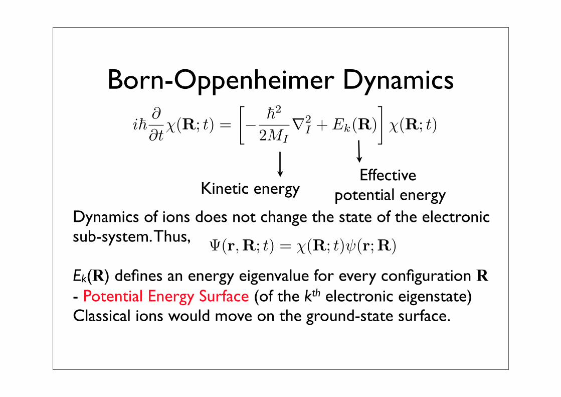
Born-Oppenheimer Dynamicsi� ∂

∂tχ(R; t) =

�− �22MI

∇2I + Ek(R)

�χ(R; t)

Kinetic energy Effective

potential energy Dynamics of ions does not change the state of the electronic sub-system. Thus,

Ek(R) defines an energy eigenvalue for every configuration R - Potential Energy Surface (of the kth electronic eigenstate)Classical ions would move on the ground-state surface.

Ψ(r,R; t) = χ(R; t)ψ(r;R)

Classical Dynamics for ionsLet’s define a classical Lagrangean for B-O dynamics

Equations of motion are obtained by

Thus we haveMIR = −∇IEBO(R)

EBO = �ψ0|He|ψ0� = minψ

�ψ|He|ψ�

LBO =1

2MIR

2I − EBO(R)

d

dt

∂

∂RLBO − ∂

∂RLBO = 0

The potential energy at every instant is obtained by solving the electronic problem variationally.

DFT Energy and Forces

Where the first term is just the DFT energy computed from the ground-state density n(r) by methods discussed earlier in this school.

Hellmann-Feynman forces :

Fi = −∇IEBO = −�

drn(r)∇IVext(r)−∇IEII(R)

External potential on electrons

EBO(R) = EDFT (R) + EII(R) = Etot

B-O Molecular Dynamics

• At every time step we need to perform a minimization to reach self consistency. This could be time-consuming (especially around 1985 where iterative diagonalization schemes were not employed for first-principles calculations).

• The accuracy of the simulation critically depends on the accuracy of the SCF minimization. (Energy drifts)

• The performance depends on the algorithms used to extrapolate the wavefunctions from the previous steps.

B-O Molecular DynamicsBO MD of butadiene molecule by two different

routes to guess initial wavefunction at each instant

P. Pulay and G. Fogarasi, Chem. Phys. Lett. 386, 272 (2004).

Energy drifts are a concern in BO MD but can be reduced by choosing good extrapolation schemes and other clever ways of

propagating the wavefunction.

Choosing parameters for MD

• A large time step means lesser overall computational cost. But need to sample fastest ionic motion. Roughly, dt ~ 0.01 - 0.1dtmax where dtmax=1/ωmax=period of fastest phonon.

• SCF convergence at each step should be very good to conserve energy, avoid systematic drifts and ensure accurate forces.

Error on DFT energy is quadratic in SCF error of charge density whereas error on forces is linear.

Some extensions

&control calculation='md' restart_mode='from_scratch', pseudo_dir = '$PSEUDO_DIR/', outdir='$TMP_DIR/', dt=20, nstep=100, disk_io='high' / &system ibrav= 2, celldm(1)=10.18, nat= 2, ntyp= 1, ecutwfc = 8.0, nosym=.true. / &electrons conv_thr = 1.0d-8 mixing_beta = 0.7 / &ions pot_extrapolation='second-order' wfc_extrapolation='second-order' /ATOMIC_SPECIES Si 28.086 Si.pz-vbc.UPFATOMIC_POSITIONS Si -0.123 -0.123 -0.123 Si 0.123 0.123 0.123K_POINTS {automatic} 1 1 1 0 0 0

1 a.u. = 2.4 * 10-17 s

iteration # 2 ecut= 8.00 Ry beta=0.70 Davidson diagonalization with overlap ethr = 4.32E-10, avg # of iterations = 2.0

total cpu time spent up to now is 0.10 secs

End of self-consistent calculation

k = 0.0000 0.0000 0.0000 ( 113 PWs) bands (ev):

-4.7636 7.1735 7.5070 7.5070

! total energy = -14.44808491 Ry Harris-Foulkes estimate = -14.44808491 Ry estimated scf accuracy < 2.8E-09 Ry

convergence has been achieved in 2 iterations

Forces acting on atoms (Ry/au):

atom 1 type 1 force = -0.02201813 -0.02201813 -0.02201813 atom 2 type 1 force = 0.02201813 0.02201813 0.02201813

Total force = 0.053933 Total SCF correction = 0.000009

Entering Dynamics: iteration = 3 time = 0.0029 pico-seconds

ATOMIC_POSITIONS (alat)Si -0.123211279 -0.123211279 -0.123211279Si 0.123211279 0.123211279 0.123211279

kinetic energy (Ekin) = 0.00015323 Ry temperature = 16.12920248 K Ekin + Etot (const) = -14.44793167 Ry

Linear momentum : 0.0000000000 0.0000000000 0.0000000000

Writing output data file pwscf.save

second order wave-functions extrapolation second order charge density extrapolation

References

• Most of the equations have been taken from D. Marx and J. Hutter, “Ab initio molecular dynamics”, Cambridge University Press, 2009

• Part of the material has been adapted from P. Giannozzi’s tutorial on QEhttp://www.fisica.uniud.it/~giannozz/QE-Tutorial/

• The original CP paper is R. Car and M. Parrinello, Phys. Rev. Lett. 55, 2471 (1985).