Ab initio assessment of computational thermodynamicsapplied to magnetic alloys

Adie Tri Hanindriyo

Japan Advanced Institute of Science and Technology

Doctoral Dissertation

Ab initio assessment of computational thermodynamics applied tomagnetic alloys

Adie Tri Hanindriyo

Supervisor : Ryo Maezono

Graduate School of Advanced Science and TechnologyJapan Advanced Institute of Science and Technology

Material ScienceMarch, 2021

Abstract

As a highly important system both in the academic and the industrial world, there is great interest in informa-tion surrounding the Nd-Fe-B ternary system. Its importance is largely derived from one of its ternary phase, theNd2Fe14B, which is used as the base compound for the most powerful permanent magnet materials available today.Alloying Nd2Fe14B with other elements (substitution in atomic sites) has long been a reliable method to engineermaterial properties suitable for various uses. A famous example is the Nd2Fe14−xCoxB compound, which substi-tutes several iron (Fe) sites with cobalt (Co) in order to increase the Curie temperature (TC), effectively increasingthe working temperature of the resulting permanent magnet. Another would be the substitution of neodymium(Nd) sites with dysprosium (Dy) in order to raise the coercivity, or resistance to demagnetization by an externalopposing magnetic field. Such efforts have largely produced the types of permanent magnet materials currentlyused in academic and industrial instruments.

Issues concerning the phase stability often arise when atomic substitution is performed, since substitution in-volves intorducing stress and strain to the atomic crystal structure of an otherwise stable phase. Often, atomicsubstitution results in symmetry breaking, additional charges, and most severely destabilization of the phase. It isimperative therefore that full information regarding phase stability is obtained prior to organizing atomic substi-tution. Phase diagrams, therefore, are indispensable to this endeavor, and as such the CALPHAD (Calculation ofPHAse Diagrams) method of computational thermodynamics is highly relevant as a computational framework todraw these diagrams. The core of the CALPHAD framework is the modelling of Gibbs energy models of the com-peting phases in a system in order to reliably model phase transitions occuring under certain conditions (pressure,temperature, composition, etc.), in order to draw the phase diagram as a function of these conditions. In this workthe temperature T and composition x are taken as the two degrees of freedom for the phase diagrams.

In order to ensure reliability of the models, parameters are built in to the Gibbs energy models used in CAL-PHAD in order to perform fitting to actual thermodynamic data of constituent phases within a system. This ensuresthat the resulting modes accurately represent the phase stability of the competing phases, leading to a more accurateand realiable prediction of phase transitions. The data used for the fitting process has traditionally been obtainedfrom experimental studies; however, while previous assessments of the Nd-Fe-B ternary system exist, the lack ofexperimental data regarding constituent phases of the Nd-Fe-B system has hampered the effort so far. In this work,we introduce ab initio predictions of thermodynamic properties of Nd-Fe-B to the CALPHAD assessment of thebinary Nd-B system, one of the constituent systems in the Nd-Fe-B ternary system, which within the CALPHADframework is necessary in order to investigate the ternary system as a whole.

Therefore, ab initio calculations of thermodynamic properties of compounds in the Nd-Fe-B ternary systemand the Fe-B, Nd-B, and Nd-Fe binary systems are required to provide more complete information for CALPHADassessment of the ternary system. The Fe-B binary system, being relatively well-investigated (due to its role in thesteel industry), is excluded from the scope of this work. Two thermodynamic properties, the enthalpy of formationand the specific heat in constant pressure (Cp), are particlarly relevant in the investigation, for the fitting of Gibbsenergy models in CALPHAD. Density Functional Theory (DFT), as well as phonon calculation, are used as abinitio investigation methods to obtain the two properties for a variety of Nd-Fe-B constituent phases.

These calculations have been performed for the compounds NdB6, NdB4, Nd2B5, Nd2Fe17 and Nd5Fe2B6.We find that the conventional exchange correlation functional GGA (Generalized Gradient Approximation) in theDFT framework is insufficient to reliably obtain the enthalpy of formation for rare earth compounds. Instead, theHubbard U correction based on the framework of Cococcioni and de Gironcoli (DFT+U) is employed, with valuesof the correction parameter Ueff determined from ab initio as well. The enthalpy of formation values obtained withthe GGA+U correction shows better agreement with the available experimental data than the non-corrected GGA.We have also computed the vibrational and electronic contribution to the heat capacity (Cp) of the compounds asa function of temperature from 0 < T < 3000 K. The results are fitted as a sum of functions from 300 < T < 3000K. Both the enthalpies of formation and Cp data have been utilized to reoptimize the Gibbs energy models for thebinary Nd-B system, leading to a reoptimized phase diagram of the system.

Keywords: CALPHAD, ab initio, Nd-Fe-B, permanent magnets, phase diagram

i

Contents

Abstract iList of Figures . . . . . . . . . . . . . . . . . . . . . . . . . . . . . . . . . . . . . . vList of Tables . . . . . . . . . . . . . . . . . . . . . . . . . . . . . . . . . . . . . . vi

1 Introduction 11.1 Background . . . . . . . . . . . . . . . . . . . . . . . . . . . . . . . . . . . . 11.2 Motivation . . . . . . . . . . . . . . . . . . . . . . . . . . . . . . . . . . . . . 21.3 Problem Statements . . . . . . . . . . . . . . . . . . . . . . . . . . . . . . . . 21.4 Outline . . . . . . . . . . . . . . . . . . . . . . . . . . . . . . . . . . . . . . 3

2 Methodology 52.1 Density Functional Theory (DFT) . . . . . . . . . . . . . . . . . . . . . . . . 6

2.1.1 Self-consistent iteration . . . . . . . . . . . . . . . . . . . . . . . . . 72.1.2 Hubbard U correction (DFT+U) . . . . . . . . . . . . . . . . . . . . . 142.1.3 Forces and phonon calculation . . . . . . . . . . . . . . . . . . . . . . 20

2.2 CALPHAD . . . . . . . . . . . . . . . . . . . . . . . . . . . . . . . . . . . . 252.2.1 Gibbs energy modeling . . . . . . . . . . . . . . . . . . . . . . . . . . 262.2.2 Parameter fitting . . . . . . . . . . . . . . . . . . . . . . . . . . . . . 272.2.3 Drawing the phase diagram . . . . . . . . . . . . . . . . . . . . . . . 28

3 Research Objective 293.1 Permanent Magnets . . . . . . . . . . . . . . . . . . . . . . . . . . . . . . . . 293.2 Overview of the Nd-Fe-B system . . . . . . . . . . . . . . . . . . . . . . . . . 30

3.2.1 Fe-B system . . . . . . . . . . . . . . . . . . . . . . . . . . . . . . . 313.2.2 Nd-Fe system . . . . . . . . . . . . . . . . . . . . . . . . . . . . . . . 313.2.3 Nd-B system . . . . . . . . . . . . . . . . . . . . . . . . . . . . . . . 323.2.4 Nd-Fe-B system . . . . . . . . . . . . . . . . . . . . . . . . . . . . . 32

4 Results and Discussion 344.1 Unary phases . . . . . . . . . . . . . . . . . . . . . . . . . . . . . . . . . . . 34

4.1.1 Nd . . . . . . . . . . . . . . . . . . . . . . . . . . . . . . . . . . . . . 344.1.2 Fe . . . . . . . . . . . . . . . . . . . . . . . . . . . . . . . . . . . . . 354.1.3 B . . . . . . . . . . . . . . . . . . . . . . . . . . . . . . . . . . . . . 35

4.2 Binary phases . . . . . . . . . . . . . . . . . . . . . . . . . . . . . . . . . . . 364.2.1 NdB6 . . . . . . . . . . . . . . . . . . . . . . . . . . . . . . . . . . . 364.2.2 NdB4 . . . . . . . . . . . . . . . . . . . . . . . . . . . . . . . . . . . 384.2.3 Nd2B5 . . . . . . . . . . . . . . . . . . . . . . . . . . . . . . . . . . . 404.2.4 Nd2Fe17 . . . . . . . . . . . . . . . . . . . . . . . . . . . . . . . . . . 41

4.3 Ternary phases . . . . . . . . . . . . . . . . . . . . . . . . . . . . . . . . . . 42

ii

4.3.1 Nd5Fe2B6 . . . . . . . . . . . . . . . . . . . . . . . . . . . . . . . . . 434.4 CALPHAD assessment . . . . . . . . . . . . . . . . . . . . . . . . . . . . . . 44

5 Conclusion 47

iii

List of Figures

1.1 Simplified workflow of the CALPHAD method, as well as the role of ab initioassessments in a combined framework . . . . . . . . . . . . . . . . . . . . . . 3

2.1 k-point grid density convergence for the unary Boron bulk calculation . . . . . 102.2 Fermi-Dirac function for k0 = 0 and various values of σ . . . . . . . . . . . . . 112.3 σ convergence for Nd2Fe17 . . . . . . . . . . . . . . . . . . . . . . . . . . . . 122.4 Linear regressions of orbital occupation, for the ’bare’ and ’converged’ series,

for NdB6 Hubbard site . . . . . . . . . . . . . . . . . . . . . . . . . . . . . . 192.5 Schematic representation of LDA energy profile, the correct (piecewise con-

stant) exact DFT energy profile for fractional occupations, and correction byHubbard U [1] . . . . . . . . . . . . . . . . . . . . . . . . . . . . . . . . . . 20

2.6 Schematic representation of periodic simulation cells with indices i and atomicpositions j . . . . . . . . . . . . . . . . . . . . . . . . . . . . . . . . . . . . . 22

2.7 Schematic workflow of phonon calculations in this work . . . . . . . . . . . . 25

3.1 Calculated phase diagram of the Fe-B system, thermodynamic assessment byVan Ende and Jung [2] . . . . . . . . . . . . . . . . . . . . . . . . . . . . . . 31

3.2 Calculated phase diagram of the Nd-Fe system, thermodynamic assessment byVan Ende and Jung [2] . . . . . . . . . . . . . . . . . . . . . . . . . . . . . . 32

3.3 Calculated phase diagram of the Nd-B system, thermodynamic assessment byVan Ende and Jung [2] . . . . . . . . . . . . . . . . . . . . . . . . . . . . . . 33

3.4 An isothermal slice at 25◦C of the phase diagram of the Nd-Fe-B system, ther-modynamic assessment by Hallemans et al [3] . . . . . . . . . . . . . . . . . . 33

4.1 Unit cell of ground state Nd . . . . . . . . . . . . . . . . . . . . . . . . . . . . 344.2 Unit cell of ground state Fe . . . . . . . . . . . . . . . . . . . . . . . . . . . . 354.3 Unit cell of αB phase . . . . . . . . . . . . . . . . . . . . . . . . . . . . . . . 354.4 Unit cell of NdB6 phase . . . . . . . . . . . . . . . . . . . . . . . . . . . . . . 364.5 Cp from phonon calculation of NdB6, in comparison with experimental result . 374.6 Cp from phonon calculation of NdB6, in comparison with estimation from the

work of Bolgar et al. [4] . . . . . . . . . . . . . . . . . . . . . . . . . . . . . 384.7 Unit cell of NdB4 phase . . . . . . . . . . . . . . . . . . . . . . . . . . . . . . 384.8 Cp from phonon calculation of NdB4, in comparison with estimation from the

work of Bolgar et al. [4] . . . . . . . . . . . . . . . . . . . . . . . . . . . . . 394.9 Unit cell of Nd2B5 phase . . . . . . . . . . . . . . . . . . . . . . . . . . . . . 404.10 Cp from phonon calculation of Nd2B5 . . . . . . . . . . . . . . . . . . . . . . 414.11 Unit cell of Nd2Fe17 phase . . . . . . . . . . . . . . . . . . . . . . . . . . . . 414.12 Cp from phonon calculation of Nd2Fe17 . . . . . . . . . . . . . . . . . . . . . 434.13 Unit cell of Nd5Fe2B6 phase . . . . . . . . . . . . . . . . . . . . . . . . . . . 434.14 Cp from phonon calculation of Nd5Fe2B6 . . . . . . . . . . . . . . . . . . . . 44

iv

4.15 Calculated Cp/T plot for NdB6. An unusual peak is seen around T = 50 K,followed by the more expected linear section. . . . . . . . . . . . . . . . . . . 45

4.16 Calculated phase diagram of the Nd-B binary system for T > 300 K, utilizingab initio calculation results in this work . . . . . . . . . . . . . . . . . . . . . 46

v

List of Tables

4.1 NdB6 Formation Enthalpy . . . . . . . . . . . . . . . . . . . . . . . . . . . . 364.2 NdB4 Formation Enthalpy . . . . . . . . . . . . . . . . . . . . . . . . . . . . 394.3 Nd2B5 Formation Enthalpy . . . . . . . . . . . . . . . . . . . . . . . . . . . . 404.4 Nd2Fe17 Formation Enthalpy . . . . . . . . . . . . . . . . . . . . . . . . . . . 424.5 Nd5Fe2B6 Formation Enthalpy . . . . . . . . . . . . . . . . . . . . . . . . . . 44

5.1 Summary of formation enthalpies Eform obtained from first-principle calcula-tions, with available experimental results for comparison . . . . . . . . . . . . 47

vi

Chapter 1

Introduction

1.1 BackgroundThe CALPHAD method (CALculation of PHAse Diagrams) [5] is a mainstay in the field ofComputational Thermodynamics. Its usefulness in the academic and industrial worlds is due toits capacity to model and predict phase transitions, and subsequently draw the phase diagramfrom simple thermodynamic information. Researchers and engineers alike frequently depend onthe phase diagram in order to investigate or design materials, as it provides vital information forcontrolling the composition and microstructure of compounds. CALPHAD’s flexibility has alsoallowed researchers to apply it to various systems and alloys, producing a large body of work(and a journal) dedicated to this method in the computational thermodynamics community.

Relatively recently, the field of CALPHAD has intersected with that of ab initio or first-principles calculation, which seeks to theoretically predict the properties of quantum systemsby numerical solutions of the Schrodinger equation. The appeal of ab initio methods overexperimental measurements are twofold: first and foremost, theoretical methods do not requireas much time, energy, or financial investments as do experimental measures. Secondly, abinitio methods have more freedom with respect to the object of investigation than empiricalmethods. For example, whereas environmental factors need to be controlled very carefullyin experimental conditions, ab initio methods simply impose different boundary conditions incalculations. CALPHAD researchers regularly include both experimental measurements andtheoretical predictions in the fitting of Gibbs energy models.

A popular example is that of the Nd-Fe-B ternary system, which has among its compoundsthe Nd2Fe14B alloy. It is often utilized, due to its high magnetisation, as a base alloy for thestrongest permanent magnets. [6] In practice however, it is often alloyed with other compoundsin order to improve its working performance. A well-known example is micro-alloying withDy [7] in order to raise coercivity. These improvements require reliable thermodynamic dataand reliable modeling in order to accurately predict phase transitions and stability. There is how-ever little experimental information regarding constituent systems (and the phases contained)of Nd-Fe-B system, which is where ab initio has a role to play.

Density Functional Theory (DFT) is regularly utilized among researchers in ab initio calcu-lation field due to the balance of feasibility and reliability it brings to the table. [8] It has beenused in previous works to predict from first-principles thermodynamic properties of compoundswhich led to reoptimization of the Gibbs energy models in CALPHAD. [9] In this manner,the DFT-CALPHAD framework has been successfully utilized to plot the phase diagram of asystem from first-principles. This approach has served to provide a more complete view of

1

materials which have traditionally been inhibited by experimental constraints (phases eithermetastable or hard to synthesize).

1.2 MotivationCALPHAD, in essence, is a framework within computational thermodynamics for modellingphase transitions using Gibbs energy models using parameters fitted to thermodynamic data of asystem’s constituent phases. The fitting process hinges upon a reliable collection of these data,and often the user of CALPHAD has to prioritize one data point over another due to measure-ment inaccuracies or other uncertainties inherent to the methodology. Experts have classicallyused a weighting scheme to take into account the reliability of available thermodynamic data;the more reliable the data, the larger weight is assigned to it during the fitting process, and fromthat follows a more reliable Gibbs energy model and phase diagram. While more reliable datadesired as a matter of course, generally speaking, it is desirable to provide as much data pointsas possible in order to allow for personal discernment from the CALPHAD user.

In this sense, DFT stands to provide valuable, reliable input to the parameter fitting processin CALPHAD. This is true especially as investigations in the academic field start to move to-ward unknown territory (machine learning, materials searching) where ab initio theoretical pre-dictions are practically vital as experimental measurements for a large number of compoundsbecome increasingly unfeasible. There is ample motivation to provide a robust framework offirst-principles investigation that is able to be applied rigorously across a large number of sys-tems while maintaining a reasonable computational cost. Therefore, first-principles frameworkssuch as DFT-CALPHAD are of great value to the field of computational thermodynamics andmaterials science alike.

Case studies for the application of these frameworks are ideally well-suited to their advan-tages over classical approaches to CALPHAD. The Nd-Fe-B system is chosen due to the lackof available thermodynamic data with regards to some of the constituent phases and systems.For example, while the constituent Fe-B binary system is rather well-documented and well-known [10, 11], the Nd-Fe and Nd-B binary systems are less well-investigated. The same canbe said for the ternary compounds within the system itself, making the Nd-Fe-B system a goodcase where first-principles investigation can bring much-needed data to improve the Gibbs en-ergy modeling. Seeing its industrial and economic importance as well, it also stands to showhow first-principles frameworks can more widely impact the world beyond academic fields.

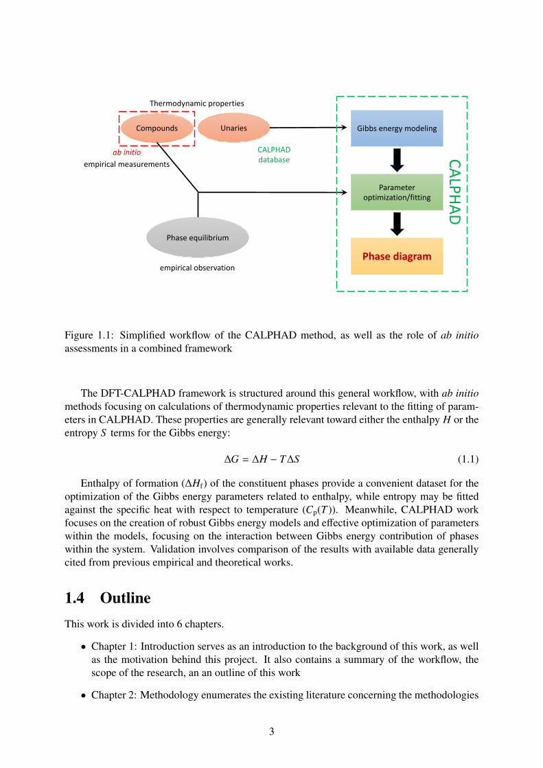
1.3 Problem StatementsConcisely put, the method of CALPHAD involves construction of Gibbs energy models, theoptimization or fitting of parameters within these models, and the use of said models to com-putationally predict phase transitions across a range of environmental variables (such as tem-perature T , pressure P, or composition). In order to build reliable Gibbs energy models for asystem, the fitting process requires parameters within the models to be optimized according tophase equilibria and thermodynamic properties of constituent compounds within the system.As shown in Figure 1.1, thermodynamic properties of compounds can be predicted by ab initiomethods, which can subsequently be utilized in the parameter fitting of Gibbs energy mod-els. Meanwhile, the Gibbs energy contribution of unaries are generally taken from the unarydatabase in CALPHAD, forming the first mathematical terms of the Gibbs energy models.

2

Compounds

Phase equilibrium

Gibbs energy modeling

Parameteroptimization/fitting

Phase diagram

Unaries

Thermodynamic properties

ab initio

empirical observation

CALPHAD database CALPHAD

empirical measurements

Figure 1.1: Simplified workflow of the CALPHAD method, as well as the role of ab initioassessments in a combined framework

The DFT-CALPHAD framework is structured around this general workflow, with ab initiomethods focusing on calculations of thermodynamic properties relevant to the fitting of param-eters in CALPHAD. These properties are generally relevant toward either the enthalpy H or theentropy S terms for the Gibbs energy:

∆G = ∆H − T∆S (1.1)

Enthalpy of formation (∆Hf) of the constituent phases provide a convenient dataset for theoptimization of the Gibbs energy parameters related to enthalpy, while entropy may be fittedagainst the specific heat with respect to temperature (Cp(T )). Meanwhile, CALPHAD workfocuses on the creation of robust Gibbs energy models and effective optimization of parameterswithin the models, focusing on the interaction between Gibbs energy contribution of phaseswithin the system. Validation involves comparison of the results with available data generallycited from previous empirical and theoretical works.

1.4 OutlineThis work is divided into 6 chapters.

• Chapter 1: Introduction serves as an introduction to the background of this work, as wellas the motivation behind this project. It also contains a summary of the workflow, thescope of the research, an an outline of this work

• Chapter 2: Methodology enumerates the existing literature concerning the methodologies

3

used in this work, mainly that of the DFT and CALPHAD methods. Core principlesare described, as well as unique considerations taken within this work (as well as thereasoning involved)

• Chapter 3: Research Objective discusses the Nd-Fe-B system as the objective of thiswork, including its application and available literature on the system

• Chapter 4: Results and Discussion details the results obtained within the course of re-search, as well as discussion on some points regarding the results

• Chapter 5: Conclusion serves as a brief summary of Chapters 2, 3, and 4, conciselyexpressing the main points, results, and conclusion of this work

4

Chapter 2

Methodology

One of the core principles of Quantum Mechanics is that quantum particles, unlike classicalobjects, do not behave in a fully deterministic manner. Uncertainty, it seems, is built into thequantum world, represented by the Heisenberg uncertainty principle. However, it is still possi-ble to predict (to a certain extent) the behavior of quantum particles by way of the Schrodingerequation:

−ℏ2

2m∇2Ψ (r, t) + V(r)Ψ (r, t) = iℏ

∂Ψ(r, t)∂t

(2.1)

with the two terms on the left being kinetic and potential energies, respectively. Practically,the Schrodinger equation is often separated into the time-dependent (t) and time-independent(r) forms. As quantum transitions often take place in a fraction of a second, most of the timeit is much more important to obtain the steady-state solution. More often than not, physicistscontend with the time-independent Schrodinger equation (colloquially abbreviated as TISE):

−ℏ2

2m∇2ψ(r) + V(r)ψ(r) = Eψ(r) (2.2)

as an eigenvalue problem with the Hamiltonian operator H, again consisting of the kinetic andpotential terms as: (

−ℏ2

2m∇2 + V(r)

)ψ(r) = Hψ(r) = Eψ(r) (2.3)

Analytic solutions are difficult to come by, however, as the effort required to solve Equa-tion 2.3 scales poorly with number of quantum particles. For a quantum system with N quantumparticles, the TISE shifts into a 3N-dimension differential equation, which is almost impossibleto solve analytically. This is the main reason why analytic solutions are only available for a se-lect few cases where only several particles in simple potentials are involved (particle-in-a-box,harmonic oscillator, hydrogen and helium atoms), whereas even for the simplest molecules theymay be just out of reach.

While there are already reliable methods to find numerical solutions of ψ(r) for second-orderdifferential equations, the computational effort required scales very poorly with the number ofparticles. Therefore, any methodology aiming to solve the TISE necessarily include approxi-mations which must aim to balance feasibility and reliability to some degree. First-principlesor ab initio methods were developed with the main goal to seek out numerical solutions to theSchrodinger equation efficiently, without relying on parameters with values taken from empir-

5

ical observations (unlike semi-empirical methods). Growth in this field has led to successfultheoretical calculations of systems of up to N = 10000 particles, which has played an instru-mental role in physics, chemistry, and microbiology (simulations of DNA [12,13], for example).

In order to reduce the complexity of the many-body Schrodinger equation, it is useful toconsider the massive difference in kinetic energy between electrons and nuclei. The large dif-ference in mass between the two particles mean that it is possible to approximate quantumsystems as comprised of high velocity electrons around stationery nuclei. Essentially, the quan-tum system with M nuclei is seen as a sequence of potential energy surfaces E(R1,R2, ..,RM)at different nuclei locations R1,R2, ..,RM. This is a famous approximation know as the Born-Oppenheimer approximation [8], which neatly separates the electronic and nucleic terms withinthe Hamiltonian:−ℏ2

2m

N∑i=1

∇2i +

N∑i=1

∑j<i

V(ri, r j) +N∑

i=1

U(ri : R1,R2, ..,RM))

ψ(r) = Eψ(r) (2.4)

with V(ri, r j) the potential from interacting electrons i and j and U(ri : R1,R2, ..,RM) thepotential energy surface with respect to nuclei positions (electron-ion and ion-ion interactions).Most ab initio methods make use of the Born-Oppenheimer approximation and consider onlyelectrons as the quantum particles in the system, separating the electron-electron, electron-ion,and ion-ion potential energy terms in the Hamiltonian.

2.1 Density Functional Theory (DFT)Density Functional Theory (DFT) was developed from the pioneering works of Hohenberg,Kohn, and Sham [14,15] in the 1960’s and has since been proven to be one of the most powerfultools available to physicists among other ab initio methods. Hohenberg and Kohn’s work [14]produced conclusions referred to today as the Hohenberg-Kohn theorems, which form the coreprinciples of DFT. The first theorem, as summarized in the book “Density Functional Theory:A Practical Introduction” by Sholl and Steckel:

“The ground-state energy from Schrodinger’s equation is a unique functional of the electrondensity.” [8]

states that it is possible to map distributions of electron density n(r) to unique values of ground-state energy E. In other words, for any quantum system, there must exist a functional of electrondensity which produces the ground-state energy E[n(r)]. Practically speaking, this is a very con-venient fact as the many-body problem of finding the solution of E(r1, r2, .., rN) for a quantumsystem of N electrons can theoretically be perfectly converted to that of finding the true densityfunctional E[n(r)], greatly reducing the complexity from a 3N-dimensional differential equationto a 3-dimensional one (r = (rx, ry, rz)). Coupled with the second theorem, again as summarizedby Sholl and Steckel:

“The electron density that minimizes the energy of the overall functional is the true electrondensity corresponding to the full solution of the Schrodinger equation.” [8]

means that it is theoretically possible to obtain the solution to the Schrodinger equation byvariationally minimizing the density functional E[n(r)].

6

Kohn and Sham would later discover the Kohn-Sham equation [15], which converts themany-body Schrodinger equation into a system of non-interacting electrons represented bysingle-particle wavefunctions ψi(r):(

−ℏ2

2m∇2 + V(r) + VH(r) + VXC(r)

)ψi(r) = ϵiψi(r) (2.5)

The potential terms from the many-body Hamiltonian is split into three parts: the nuclei-electronpotential V(r), the Hartree potential (electron-electron) VH(r), and the exchange-correlationfunctional VXC(r). The Kohn-Sham equation is in practice solved iteratively with a fractionof the effort it takes to solve the full many-body Schrodinger equation. The reliability of thisframework largely relies on how exact the density functional E[n(r)] is to the true form ofthe density functional, largely represented by the “unknown” form of the exchange-correlationfunctional VXC(r).

To summarize the fundamental principles of DFT, the electron density n(r) can be uniquelymapped to the ground state energy E, forming the density functional E(n(r)). By variationalminimization of the E(n(r)), it is possible to obtain the true electron density n(r) of the quantumsystem. Finally, by converting the many-body problem of the Schrodinger equation to a seriesof single-particle Kohn-Sham equations, computational solving of the many-body problem be-comes feasible.

From the Hohenberg-Kohn theorem, it is proven that the conversion from the many-bodySchrodinger equation to the Kohn-Sham equations can be exact (without error). However, prac-tically speaking, this exact conversion is not achievable due to forms of electron interaction notproperly accounted in the Kohn-Sham equation. The term VXC(r) in the Kohn-Sham equationis the exchange-correlation (XC) functional which describes exchange interactions and electroncorrelation, and represents the “unknown” mathematical forms of electron interaction from themany-body problem.

2.1.1 Self-consistent iterationBeginning with an initial guess of the electronic density n(r), the Kohn-Sham equations aresolved by matrix diagonalization in order to produce the single-particle eigenfunctions ψi(r).The computation results are used to re-calculate the new electronic density n∗(r), which is thencompared with the initial guess n(r). If the difference between the two electronic densitiesexceed a certain tolerance value, the calculation enters a new iteration by utilizing some form ofmixing between the initial and new electron densities. The loop proceeds in the same manneruntil the difference between old and new densities falls below the tolerance value, in which casethe density is said to be ‘self-consistent’ and the loop ends, resulting in the electron density n(r)corresponding to the true ground state electronic density.

Despite the seeming simplicity of the core process of DFT, practically there are deeper con-siderations that must be taken beyond the choice of the exchange-correlation functional (whilebeing an important factor in and of itself). In fact, these considerations contribute significantlyto the reliability of DFT for any certain system, and is quite common to be the source of signif-icant error when neglected. These basic practical considerations are described in the book bySholl and Steckel [8] and briefly discussed here:

7

Basis set

Within quantum mechanics, the state of quantum particle is embodied within a mathematicalfunction known as the wavefunction. They are typically represented by the basis set, whichis a set of basis functions representation of the wavefunction. Expanding the basis set allowsthe wavefunction to be more rigorously represented, and more complexity within its behaviorcaptured in its representation. Practically, physicists and chemists would choose a set of basisfunctions that best model their system and the extent of the basis set expansion. The completebasis set (CBS) limit is defined as the extent of basis set expansion which is equivalent to aninfinitely large basis set, usually obtained from extrapolation from multiple sizes of basis set.Realistically however, a tolerance value is generally adopted in order to balance computationalfeasibility and accuracy; for example, at the level of chemical accuracy (around 1 kcal/mol).

Plane-wave basis set is often utilized in systems with periodic boundary conditions, fullytaking advantage of the periodic nature of plane waves. Therefore, calculations of bulk com-pounds (infinitely periodic in 3D) or surfaces (periodic in 2D) often use plane-wave basis setto represent the electronic wavefunction. Equation 2.6 shows a general plane-wave basis setexpanded in wavevector k, arising from the Fourier transform from real-space coordinates r:

ψi(r) =∑

k

ci(k)eik·r (2.6)

The term “cutoff energy” of plane-wave basis set is used to set the extent of the basis set ex-pansion. Higher energy plane waves (with larger wavevector k) represent diminishingly smallcontributions (in general) to the overall wavefunction. In computational calculations, the con-tribution of plane waves beyond the cutoff energy Ecut is deemed insignificant to the result ofcalculation (to within a tolerance value).

Ecut =ℏ2

2m|kmax|2 (2.7)

The cutoff energy Ecut introduces a limit to the expansion in Equation (2.6), limiting thebasis set to functions defined in Equation 2.8.

ψi(r) =∑

k<kmax

ci(k)eik·r (2.8)

First-principles calculation of bulk structure of compounds make up the overwhelming ma-jority of the calculations performed within this work. As such, the plane-wave basis set ischosen to represent the periodic electronic wavefunctions.

Reciprocal space

Taking full advantage of the periodic nature of bulk or surface calculations, it is computationallyvery efficient to perform a Fourier transform on real space coordinates and perform calculationsover the frequency domain (over the wavevectors k instead of position vectors r). The resultantcoordinates from the Fourier transform is referred to as the reciprocal space or the k-space. Itis not a concept alien to materials science, as other branches within the field (X-ray diffraction,for instance) also utilizes the reciprocal space to take advantage of crystal periodicity.

The lattice vectors of the crystal cell a1, a2, and a3 is redefined in reciprocal space by Fouriertransformation. It is notable that the real space and reciprocal space lattice vector lengths are

8

inversely proportional; a longer real space lattice vector is transformed into an inversely smallerreciprocal lattice vector according to Equation 2.9.

b1 = 2πa2 × a3

a1 · (a2 × a3)

b2 = 2πa3 × a1

a2 · (a3 × a1)

b3 = 2πa1 × a2

a3 · (a1 × a2)(2.9)

A primitive cell in reciprocal space is known as the Brillouin zone; the smallest volumewhich contains all the information necessary to reproduce crystal periodicity in 3 dimensions.Needless to say, it is computationally most efficient to work within the Brillouin zone (akin toutilizing the primitive cell as the minimum volume in real space). Practically, the irreducibleBrillouin zone (IBZ) is obtained by taking advantage of crystal symmetry in the Brillouin zonein order to further minimize the computational effort.

In computation, numerical solutions of integrals over variable x is approximated as sumsover discrete values of x. In the same way, integrations over wavevectors k is discretized assummations over a selection of points in the Brillouin zone (oft referred to as k-points). Theconcept of k-mesh is very important in ab initio calculations as a grid of k-points in the recip-rocal space, over which summations are performed to numerically solve analytic integrals. Dueto the nature of the reciprocal space, each k-point may be weighted differently depending on itssignificance to the crystal structure and crystal symmetry.

The Monkhorst-Pack [16] scheme of k-mesh generation is often used for identifying relevantk-points in the Brillouin zone. There is a computational need to carefully balance the density ofthe k-mesh. While denser k-mesh is ideal in order to more reliably approximate integrals overthe IBZ, it also increases the computational cost to calculate over a larger set of k-points. Wherehigh frequency oscillations of the wavefunction occur (higher energy terms in the basis set), adenser collection of k-points is also required. As with the cutoff energy Ecut, it is desirable toincrease the k-mesh density up to a certain point above which increasing the number of k-pointsdoes not significantly impact the accuracy of calculations.

Parameter convergence

The cutoff energy Ecut and k-mesh density are two important parameters which determinesthe cost and accuracy of DFT calculations. It is therefore standard practice to measure theconvergence of at least both of these parameters before starting a production (actual) calculation.Often times the ground state energy of the quantum system (colloquially the “Total energy”)is used as a measurement for convergence of calculation results with respect to calculationparameters.

Figure 2.1 shows an example of total energy convergence with respect to k-mesh densityfor the unary Boron ground state. Several quick single-point calculations are performed, withdiffering M×M×M k-mesh (M points along a reciprocal lattice axis), and the change in the totalenergy is apparent. Adopting a tolerance value of 1 mRy (well below the chemical accuracy of1 kcal/mol ≈ 3 mRy) it can be seen that the value of M = 4 is enough to achieve convergencebelow the tolerance value. The addition of M above M = 4 does not contribute significantly tothe total energy and as such merely serves to increase the computational cost.

9

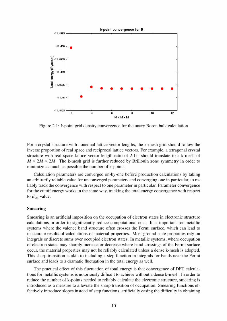
Figure 2.1: k-point grid density convergence for the unary Boron bulk calculation

For a crystal structure with nonequal lattice vector lengths, the k-mesh grid should follow theinverse proportion of real space and reciprocal lattice vectors. For example, a tetragonal crystalstructure with real space lattice vector length ratio of 2:1:1 should translate to a k-mesh ofM × 2M × 2M. The k-mesh grid is further reduced by Brillouin zone symmetry in order tominimize as much as possible the number of k-points.

Calculation parameters are converged on-by-one before production calculations by takingan arbitrarily reliable value for unconverged parameters and converging one in particular, to re-liably track the convergence with respect to one parameter in particular. Parameter convergencefor the cutoff energy works in the same way, tracking the total energy convergence with respectto Ecut value.

Smearing

Smearing is an artificial imposition on the occupation of electron states in electronic structurecalculations in order to significantly reduce computational cost. It is important for metallicsystems where the valence band structure often crosses the Fermi surface, which can lead toinaccurate results of calculations of material properties. Most ground state properties rely onintegrals or discrete sums over occupied electron states. In metallic systems, where occupationof electron states may sharply increase or decrease where band crossings of the Fermi surfaceoccur, the material properties may not be reliably calculated unless a dense k-mesh is adopted.This sharp transition is akin to including a step function in integrals for bands near the Fermisurface and leads to a dramatic fluctuation in the total energy as well.

The practical effect of this fluctuation of total energy is that convergence of DFT calcula-tions for metallic systems is notoriously difficult to achieve without a dense k-mesh. In order toreduce the number of k-points needed to reliably calculate the electronic structure, smearing isintroduced as a measure to alleviate the sharp transition of occupation. Smearing functions ef-fectively introduce slopes instead of step functions, artificially easing the difficulty in obtaining

10

a self-consistent solution for the charge density n(r). Equation 2.10 shows an example of theFermi-Dirac smearing function:

f(k − k0

σ

)=

1

exp(

k−k0σ

)+ 1

(2.10)

as a sloped step function at k = k0 depending on the value of σ. Figure 2.2 shows the Fermi-Dirac smearing function with various values of smearing parameter σ. It can be seen that largervalues of σ increases the slope of the function at k = k0.

Figure 2.2: Fermi-Dirac function for k0 = 0 and various values of σ

Various smearing functions exist and within this work, the Marzari-Vanderbilt cold smear-ing [17] is used to broaden the occupation by convolution with a delta function:

δ(x) =2√π

e−[x−

(1√2

)]2 (2 −√

2x)

(2.11)

As an artificial imposition on the wavefunction, it is desirable to limit the smearing pa-rameter σ to as small as possible to preserve the accuracy of the calculation. Practically, it isconverged in the same way as cutoff energy and k-mesh density, as shown in Figure 2.3.In this example, it is shown that values of smearing parameter σ beyond 0.03 Ry more sig-nificantly affects the total energy, which limits the smearing parameter to 0.03 Ry to help theself-consistent requirement.

Pseudopotential

An early conclusion in chemistry is that elements in the same periodic table group tend tobehave in a similar chemical manner. The grouping of elements in the periodic table reflectsthe valence electrons in an atom which, as a result of being weakly bonded to the nucleus, areeasily transferred or shared between atoms, forming chemical bonds (ionic, covalent). In short,

11

Figure 2.3: σ convergence for Nd2Fe17

valence electrons carry far more significance in chemical bonding than the more tightly boundcore electrons.

The field of quantum chemistry takes advantage of this physical fact by employing pseu-dopotentials in place of core electrons. These pseudopotentials reproduce the screening ofvalence electrons by core electrons, effectively removing the need to include core electrons inelectronic structure calculations. Pseudopotentials are constructed so that up to a cutoff radiusof rc from the nucleus, the wavefunction is approximated by a simpler smoothed function whichreproduces the behavior of a core electron, and simply recreates the valence electron wavefunc-tion beyond the cutoff radius. The advantage of this “frozen-core” approximation is twofold:

• Removing the core electrons from consideration is vital for calculations of heavy ele-ments, for which all-electron calculations (without pseudopotentials) are computationallyunfeasible. This is also true for large quantum systems where all-electron calculationsscale very poorly with the number of particles.

• Higher energy core electrons possess rapidly oscillating wavefunctions near the nucleus,which must be represented by higher expansions in the basis set. By excluding coreelectrons from consideration, the expansion of basis set can be stopped in lower energies,again reducing the computational cost of electronic structure calculations greatly.

Various forms of pseudopotentials exist with its own strengths and weaknesses. Two promi-nent types of pseudopotentials are the norm-conserving (NC) pseudopotentials and the projec-tor augmented-wave (PAW). Norm-conserving pseudopotentials [18,19] are so called due to therequirement of preserving the charge density of the all-electron core within the cutoff radius.While ensuring good transferability, this also requires higher energy expansions of the basisset, which is referred to as the “hardness” of the pseudopotential. Meanwhile, the projectoraugmented-wave pseudopotentials [20,21] are softer in comparison and much more commonlyused recently due to their efficiency.

12

Exchange-correlation potentials

As previously mentioned the exchange-correlation functional is the single most important ap-proximation within DFT. This is due to the unknown form of the exchange-correlation func-tional which must be approximated, since only the existence of the true exchange-correlationfunctional has been mathematically proven. In this sense, DFT can be said to be exact, thatthere is an exact form of the exchange-correlation functional which minimizes the ground stateenergy and reproduces the real ground state charge density. It can be said that the Hamiltonianis split between the “known” and “unknown” parts of DFT, with the kinetic, electron-electron,and electron-nucleus potentials representing the “known” physical interactions. The exchange-correlation functional represents the practically “unknown” factor in DFT, and is approximatedby various functional forms, some of which might work well for some systems and not for oth-ers. The choice of exchange-correlation functional is in a sense the most important choice onthe part of the physicist in determining the reliability of DFT calculations.

One of the earliest and simplest forms of exchange-correlation functional is the Local Den-sity Approximation (LDA) [22], constructed from calculations of the homogeneous electrongas (jellium model). It is a functional of the local density n(r) at a point in space, VXC(r) =VLDA

XC [n(r)], from which it earned its name. Despite its simplicity, it has surprisingly performedwell for a wide range of systems, especially where electron density resembles that of the jelliummodel. Another form of the exchange-correlation functional is the Generalized Gradient Ap-proximation (GGA) [23], which beyond the electron density, also takes into account the gradientof electron density. In practice, GGA is more reliable than LDA for systems where sharp gra-dients of n(r) exist, such as surfaces and semiconductors. As such, GGA exchange-correlationfunctional is used in this work for DFT calculations.

The reliability of both LDA and GGA exchange-correlation functionals, while perfectlygood for a wide variety of systems, is not perfectly applicable on all quantum systems. Thereare famous examples within the ab initio community for which neither LDA nor GGA givethe correct solution, for example transition metal oxides (such as NiO [24] and graphene [25]).Practically, physicists employ different exchange-correlation functionals and different correc-tions to take into account the strengths and weaknesses of each type, choosing one which bestfits the system. A well known case of this are the strongly correlated class of materials, forexample, transition metal oxides and rare-earth elements with localized 4 f electrons, whereelectron exchange and correlation serve a more significant role in their properties. As a re-sult, conventional exchange-correlation functionals have been proven to be unable to properlypredict properties of these materials.

Other forms, such as hybrid exchange-correlation functionals, have been successfully ap-plied for these systems. [26] By introducing more accurate short-range Hartree exchange (fromHartree-Fock calculation method), hybrid exchange-correlation functionals successfully ac-count for physical effects which govern the properties of strongly correlated materials. It in-troduces, however, either arbitrary, empirical, or semi-empirical parameters (one of which isthe ratio of short vs. long range exchange) which severely limits its predictive capability as afirst principles method.

Another such solution is a simpler correction term added onto the conventional exchange-correlation functional. While seemingly simple, it has successfully been applied to stronglycorrelated materials, most notably for transition metal oxides. [27, 28] This correction termstems from another ab initio model called the Hubbard model, and as such is referred to as theHubbard correction. This method is detailed in the next section, and is specific to calculations

13

of certain localized orbitals within the valence electrons.

2.1.2 Hubbard U correction (DFT+U)A class of ’strongly correlated’ materials such as transition metal oxides (including the most fa-mous example of NiO [29]) are poorly described with regular or classical exchange-correlationfunctionals such as LDA and GGA. Mott insulators are well-known to exhibit this property, inthat LDA or GGA prediction describes them as metals while in reality these materials are insu-lators. Researchers have known of this problem for some time, and one of the solutions alongthe years is to adopt the Hubbard correction term U. [28]

The Hubbard correction term U regularly employed in DFT (oft referred to as the DFT+Umethod) stems from the Hubbard Hamiltonian, a feature of the Hubbard model. [27] As anextension of the tight-binding model, the Hubbard model is used to describe the Mott transition;a transition between metallic and insulating properties due to the Pauli repulsion of localizedorbitals. In second quantization form, it is written as follows:

HHubbard = −t∑⟨i, j⟩,σ

(c†i,σc j,σ + c†j,σci,σ

)+ U

∑i

ni↑ni↓ − µ∑

i

(ni↑ + ni↓

)(2.12)

The Hubbard model consists of electron occupation sites in a periodic lattice, where two elec-trons of opposing spin can occupy one site. The first term describes the ’hopping’ of electronsbetween adjacent sites ⟨i, j⟩ with the same spin σ, and is characterized by the hopping term t.The second term, meanwhile, introduces the energy cost U when both spins are occupied, inorder to describe the Pauli repulsion. The last term describes occupation of sites from electronchemical potential µ. To describe the changes in occupation, the second quantization notationsof c†i,σ and ci,σ are used. Known as the ‘creation’ and ‘destruction’ operators, respectively, theseoperators serve to increase and decrease the occupation of sites in the Hubbard Hamiltonian.The number operator niσ results in the occupation number of site i with spin σ, niσ = c†i,σci,σ.

As previously stated, the Pauli repulsion is the source of the Mott transition, and is describedby the on-site repulsion U in the Hubbard model (the second term in Equation 2.12). This isthe source of the Hubbard U correction, where an energy cost of magnitude U is applied whenboth spins are occupied. In Mott insulators, this mechanism gains significance and promoteshalf-filling of the valence band in the ground state, with the cost U raising the conduction bandlevel (realizing an insulating electronic structure). The same holds true for localized 3d and 4 flocalized orbitals commonly found in rare earth and several transition metal compounds, forwhich conventional exchange-correlation functionals unfortunately do not adequately capturethis phenomenon.

For DFT, the Hubbard U term is adopted as an artificial correction to the exchange-correlationfunctional in DFT+U. Within the DFT+U implementation of Anisimov, et al. [30], the U cor-rection is added onto the exchange-correlation term as a function of occupation of localizedorbitals. Two parameters, U and J, appear within this implementation, respectively controllingfor the strength of Coulomb and exchange interactions for localized orbitals, while delocalizedorbitals (s and p orbitals) are still well-described by regular DFT.

For conventional exchange correlation functionals LDA and GGA, the Hubbard term effec-tively provides a solution to the self-interaction problem. Equation 2.5 shows the Hamiltonianform of the Kohn-Sham equation, which consists of the kinetic energy and the potential energyV , the latter consisting of the Hartree term and the exchange correlation term. Strictly speaking,

14

the potential term V i j represents interaction between electrons with different quantum numbersi and j. Each electron possesses a different orbital and spin (quantum number), and naturallyterms representing interactions between electrons of the same orbital and spin (self interaction)should be taken out of the equation (i = j terms in Equation 2.13).

V i j =∑i, j

V i jH +

∑i, j

V i jXC (2.13)

However, this self interaction is included in the formulation of the Hartree term, as a rep-resentation of Coulomb interaction with a field of electron density n(r) (without distinguishingelectron orbital and spin). While it provides a relatively convenient method of integration, thegeneralized formulation also means that self interaction is included within the Hartree term. Ex-act exchange correlation functional would cancel out this self interaction present in the Hartreeterm and provides exact solutions. However, LDA and GGA exchange correlation function-als are constructed as well as a function of n(r), and as such does not provide self interactioncancellation in a rigorous manner.

While LDA and GGA has been shown to be effective enough to cancel out the self inter-action for delocalized orbitals, the self interaction error becomes quite significant for localizedorbitals. The Hubbard correction effectively serves as the penalty term to rectify this imbal-ance, specifically treating localized orbitals where this error becomes significant. The Hubbardparameters U and J, in turn, can be considered as the strength of this penalty term.

Original formulation

The original implementation of DFT+U [28–31] adds two correction terms to the exchange-correlation functional:

E[n(r)] = EDFT[n(r)] + EHub[nIσm ] − EDC[nIσ] (2.14)

As previously stated, s and p delocalized states are well described by DFT: therefore, nIσ andnIσ

m (atom I, spin σ, and magnetic moment index m) refer to the density of electrons in localizedorbitals only, which are usually 3d orbitals in transition metals and 4 f orbitals in rare earthcompounds. These orbitals are commonly referred to as “Hubbard sites”, and the second andthird terms in Equation 2.14 are exclusively applied to these orbitals as part of the DFT+Uscheme. The second term accounts for the interactions in localized orbitals, which is calculatedusing the Hubbard scheme. The third term is known as the “double counting” term, which aimsto subtract the energy of localized orbitals from the first (regular DFT) term, as the addition ofthe first and second terms mean that the energy contribution from Hubbard sites are countedtwice (once as a delocalized/regular DFT scheme in the first term, and once again in the secondterm as a Hubbard scheme). The double counting term subtracts the contribution of Hubbardsites calculated as a regular DFT scheme, as a function of electron density of a certain atom Iand spin σ (nIσ =

∑m nIσ

m ).

The original implementation of DFT+U by Anisimov et al. is well-suited for the linearmuffin-tin orbital (LMTO) basis set, but is not generalized to include other forms of basis sets.Needless to say, it is also ill-suited for the plane-wave basis set used in this work. Instead, theDudarev [24] scheme is used in this work, which is (most importantly) basis set independent,also incorporating the generalized basis set for LDA+U by Liechtenstein et al. [32] For plane-waves basis sets, eigenstates of Hubbard sites are projected onto localized basis sets and are

15

then treated with Hubbard correction. The occupation matrix elements nIσmm′ are defined as:

nIσmm′ =

∑k,υ

f σk,υ⟨ψσk,υ

∣∣∣PImm′

∣∣∣ψσk,υ⟩ (2.15)

where the eigenstates ψσk,υ corresponding to crystal momentum k, band υ, spin σ, and occupa-tion f σk,υ are projected onto pseudo-atomic (localized) wavefunctions by the generalized projec-tor PI

mm′:

PImm′ =

∣∣∣φIm

⟩ ⟨φI

m′∣∣∣ (2.16)

and for PI =∑m

PImm, the total occupation of localized orbitals for atom I,

nI =∑σ

∑k,υ

f σk,υ⟨ψσk,υ

∣∣∣PI∣∣∣ψσk,υ⟩ =∑

σ,m

nIσmm (2.17)

Liechtenstein’s formulation for the Hubbard correction term EHub (Equation 2.14) is derivedfrom screened Coulomb interactions Vee between Hubbard sites, expressed in Hartree-Fockmethod terms:

EHub

[{nI

mm′}]=

12

∑{m},σ

{⟨m,m′′ |Vee|m′,m′′′⟩ nσmm′n

−σm′′m′′′

+(⟨m,m′′ |Vee|m′,m′′′⟩ − ⟨m,m′′ |Vee|m′′′,m′⟩

)nσmm′n

σm′′m′′′

}(2.18)

with the notation in Equation 2.18 defined as:

⟨m,m′′ |Vee|m′,m′′′⟩ =∫ ∫

ψ∗lm(r)ψ∗lm′′(r)e2

|r − r′|ψlm′(r′)ψlm′′′

(r′)

drdr′ (2.19)

The double counting term EDC is defined as:

EDC

[{nI

}]=

∑I

U2

nI(nI − 1

)−

∑I

J2

[nI↑

(nI↑ − 1

)+ nI↓

(nI↓ − 1

)](2.20)

Parameters U and J describe the screened Coulomb and exchange interactions, respectively.The values of U and J were calculated by Anisimov et al. by perturbation of a constrainedoccupation matrix element nIσ

mm′ , following the preceding work of Gunnarsson et al. [33] withLMTO basis set. Cococcioni et al. [1] would go on to develop a similar method for use with theplane-wave basis set, implemented in the QUANTUM ESPRESSO code. [34]

Determination of Hubbard U

This work adopts the DFT+U implementation of Cococcioni and de Gironcoli [1], which makesuse of the effective Hubbard parameter Ueff = U − J instead, greatly simplifying the earlierscheme of Anisimov et al.By effectively ignoring the exchange parameter J, this approximationallows the calculation of the Ueff parameter from first-principles, which is quite useful in the casewhere few empirical data of the target material is available. By constraining the occupation ofa Hubbard site and introducing perturbations, the relaxation stemming from the perturbation

16

can be used to compute the Ueff parameter. The simplified energy functional, with J = 0, is asfollows:

E[n(r)] = EDFT[n(r)] + EHub

[{nI

mm′}]− EDC

[{nI

}]= EDFT[n(r)] +

Ueff

2

∑I

∑m,σ

nIσmm −

∑m′

nIσmm′n

Iσm′m

= EDFT[n(r)] +

Ueff

2

∑I,σ

Tr[nIσ

(1 − nIσ

)](2.21)

it is clear that the combined EHub and EDC can be calculated by diagonalizing the occupationmatrix for localized orbitals:

nIσvIσi = λ

Iσi vIσ

i (2.22)

with orbital occupation as eigenvalues 0 ≤ λIσi ≤ 1. The energy functional becomes:

E[n(r)] = EDFT[n(r)] +Ueff

2

∑I,σ

∑i

[λIσ

i

(1 − λIσ

i

)](2.23)

As such, the Ueff correction raises the total energy for fractional occupation (0 < λIσi < 1), and

reduces to the regular DFT functional for integer values of occupation. This is connected to thephysical meaning of the Hubbard U correction within this scheme, discussed later on.

The aforementioned correction favoring integer occupation of localized orbitals is deter-mined in magnitude by the value of parameter Ueff. Following the original implementation ofDFT+U by Anisimov et al. [30], the value of Ueff is obtained by a perturbation scheme withconstrained occupation of the Hubbard site. A slight difference is present due to the differencein basis sets used: Anisimov’s method uses LMTO representation and decouples completely thelocalized orbitals from the delocalized ones. By utilizing the same plane-wave basis set for allorbitals, the method of Cococcioni and de Gironcoli needs to separate the nonlinear change inenergy due to rehybridization of orbitals upon relaxation of the occupation-constrained local-ized orbitals. This change in energy is unrelated to the Hubbard Ueff (on-site Coulomb repul-sion) and must be subtracted from the total change in energy due to perturbation.

Lagrange multiplier αI is applied to constrain the localized orbital occupation nI , to con-struct an expression for the total energy functional as a function of this occupation:

E[{qI}

]= min

n(r),αI

E[n(r)] +∑

I

αI (nI − qI)

(2.24)

The correction parameter Ueff is contained within the curvature (second derivative) of E[{qI}

]with respect to the constraint qI . This corresponds to the energy cost of constraining integer oc-cupations in Hubbard sites. The previously mentioned change in energy due to rehybridizationis obtained from the equivalent curvature of energy with respect to occupation constraint, butwithin the Kohn-Sham non-interacting scheme:

EKS [{qI}]= min

n(r),αKSI

EKS [n(r)] +∑

I

αKSI (nI − qI)

(2.25)

17

As such, the Ueff parameter is obtained from the subtracted curvature of Equations 2.24 and 2.25,

U =∂2E

[{qI}]

∂q2I

− ∂2EKS [{qI}

]∂q2

I

(2.26)

Application of Janak theorem [35] turns the second derivatives of Equation 2.26 into firstderivatives of the eigenvalue, or αI in this case (according to Dederichs et al. [36]):

∂E[{qI}

]∂qI

= −αI ,∂EKS [{qI}

]∂qI

= −αKSI (2.27)

transforming the second derivatives in Equation 2.26 into

∂2E[{qI}

]∂q2

I

= −∂αI

∂qI,∂2EKS [{qI}

]∂q2

I

= −∂αKS

I

∂qI(2.28)

Practically speaking, in calculations it is much more useful to set the Lagrange multipliers αI

as the independent variables, which is achievable through a Legendre transform:

E[{αI}] = minn(r)

E[n(r)]∑

I

αInI

EKS

[{αKS

I

}]= min

n(r)

EKS [n(r)]∑

I

αKSI nI

(2.29)

with density response functions χIJ and χ0IJ defined as

χIJ =∂2E

∂αI∂αJ=∂nI

∂αJ

χ0IJ =

∂2EKS

∂αKSI ∂αKS

J

=∂nI

∂αKSJ

(2.30)

to represent the first-level derivative of energy in Hubbard site I with respect to perturbation insite J. Combining Equations 2.26, 2.28, and 2.30, the calculation of Ueff is obtained:

U = −∂αI

∂qI−

(−∂αKS

I

∂qI

)= − 1

χII−

(− 1χ0

II

)(2.31)

The linear response functions of perturbation αI from both interacting and non-interacting(many body and Kohn-Sham) schemes are required in order to calculate Ueff. Practicallyspeaking, both can be calculated from the relaxed and unrelaxed Hubbard site occupationsnI from perturbation αI . The unrelaxed (’bare’) occupation represents the non-interacting re-sponse, while the relaxed (’converged’) occupation represents the response of Hubbard siteunder screening effects from the other orbitals. Since the first derivatives of the occupation isrequired, a series of calculations involving various valus of αI is performed, obtaining ’bare’(first iteration) and ’converged’ (last iteration) Hubbard site occupations, and finding both linearresponse functions as slopes of linear regressions:

18

nI [{αI}] = χIIαI +CnKS

I [{αI}] = χ0IIαI + D (2.32)

The Hubbard U can then be obtained as in Equation 2.31:

U =1χ0

II

− 1χII

(2.33)

for the Hubbard site I.

Example of determination of effective Hubbard U parameter

The following is an example of the scheme for determining Ueff for the Hubbard site of NdB6.By introducing multiple perturbations in the form of the parameter α, and drawing linear re-sponse functions for both the ’bare’ and ’converged’ series (first and last iterations of the self-consistent calculations), the Ueff parameter can be determined. Using small values of pertur-bation α (-0.08, -0.06, ..., 10−40, 0.02, ..., 0.08), the Hubbard site occupations are plotted andlinear fittings are performed using the least-squares method:

Figure 2.4: Linear regressions of orbital occupation, for the ’bare’ and ’converged’ series, forNdB6 Hubbard site

Figure 2.4 shows the ’bare’ and ’converged’ linear response functions of f (α) = −1.4480α+3.5646 and g(α) = −0.6376α+ 3.5711, respectively. The parameter Ueff value is then computedaccording to Equation 2.33:

Ueff =1

−1.4480− 1−0.6376

= 5.3377 eV (2.34)

Physical meaning of Hubbard U

The physical effect of the Ueff correction is to discourage fractional occupation for the Hubbardsites. This is rooted in the physical fact that fractional occupation of a quantum system is im-

19

possible: it is only possible as a statistical average of systems with different integer occupations.For example, for a non-adiabatic system (possible to exchange electrons with the environment)with the ground state of the system having N electrons, the addition or subtraction of electrons(N+1 or N-1 electrons) would serve to increase the total energy. Fractional occupations as astatistical mixture of two states are therefore unphysical (unless the two states are somehowdegenerate) possibilities for the ground state.

For instance, for a system of N + ω electrons, with integer N and 0 ≤ ω ≤ 1, the energy:

EN+ω = (1 − ω) EN + ωEN+1 (2.35)

Figure 2.5: Schematic representation of LDA energy profile, the correct (piecewise constant)exact DFT energy profile for fractional occupations, and correction by Hubbard U [1]

This energy profile between integer occupations (piecewise constatnt) is represented in Fig-ure 2.5 and is not correctly reproduced by LDA or GGA exchange-correlation functionals,which produces continuous energy profile for fractional occupations. The Hubbard Ueff is theenergy cost to correct this unphysical behavior, which in this diagram would then correctlydetermine the integer occupation N to be the ground state instead of the unphysical fractionaloccupation. By rectifying the ground state fractional occupation, the simplified DFT+U schemeaddresses the self-interaction of half-filled localized orbitals which is fundamental to the failureof LDA and GGA for strongly correlated systems.

2.1.3 Forces and phonon calculationFrom the self-consistent iteration process of DFT, it is possible to solve the eigenvalue prob-lem in Equation 2.3, obtaining both the eigenvalue E (ground state energy) and eigenfunctionsψ(r) (spatial wavefunction) from the Hamiltonian H. The information obtainable from self-consistent iteration, therefore, is not limited to the ground state energy, but also includes allobservables obtainable from the spatial wavefunction ψ(r). This includes the atomic forces, as

20

the first derivative of energy with respect to spatial coordinates r, which plays a vital role inboth optimization of atomic geometry and calculation of atomic vibration (phonon).

The calculation of forces makes use of the Hellmann-Feynman theorem [37], an analyticprinciple discovered the 1940s for Hamiltonians which is not exclusive to DFT and also appliedin other quantum chemistry methods. The theorem establishes that derivatives of the eigenvalueis obtainable from diagonalization of derivatives of the Hamiltonian:

δEδx=

⟨ψ(x)

∣∣∣∣∣∣δHδx

∣∣∣∣∣∣ψ(x)⟩

(2.36)

In the same way, it is possible to calculate the first derivative of forces; that is, the second deriva-tive of energy with respect to spatial coordinates r. The resultant matrix of second derivativesis referred to as the Hessian matrix and is key in performing optimization of crystal geometry,discussed in the following section.

Geometry optimization

The ground state crystal structure of compounds are first optimized before reliable electronicstructure calculations may take place. Within these calculations, apart from ground state en-ergy optimization with respect to electron density (see Section 2.1.1), it must also be optimizedwith respect to atomic positions in the crystal. The Broyden-Fletcher-Goldfarb-Shanno (BFGS)algorithm is commonly used to optimize the geometry [38], and for phonon calculations it isdesirable to optimize the geometry not just with respect to the ground state energy, but alsoatomic forces as well (setting a maximum allowable value for atomic forces) as will be dis-cussed in harmonic and quasi-harmonic approximations employed in phonon calculations (seeSection 2.1.3).

The GGA exchange-correlation functional is known to reliably reproduce atomic latticeconstants for transition metals during geometry optimization, while LDA sometimes underes-timates lattice constants. There is then motivation to choose GGA over LDA when dealingwith transition metal compounds, extrapolating this accuracy toward atomic forces as well. Assuch, phonon calculations in particular benefit from proper choice of the exchange-correlationfunctional, largely stemming from the reliability of calculation of forces.

Phonon calculation

Chemical bonds between atoms in a quantum system also dictate how vibration of atomic po-sitions occur. Most importantly, these bonds couple the vibrations of one atom with others inits chemical environment. In short, in a molecule of solid, no single atom vibrates on its own.Classically, chemical bonds between atoms in a quantum system can be viewed as springs witha certain spring constant, influencing how waves propagate within the system. The collectivevibration possess normal modes with discrete levels of energy, referred to as phonons.

As photons are defined as discrete levels of electromagnetic energy, phonons are defined asthe discrete levels of vibrational energy in a quantum system. Studying phonon properties inmaterials is vital in understanding how energy propagates through said material. As such, itis important in the study of either thermal and acoustic properties of materials. One of theseproperties is the specific heat under constant pressure or Cp, which is significant due to itsrelation with the entropic term in Equation 1.1,

21

∫ T2

T1

Cp(T )T

δT = S (T2) − S (T1) (2.37)

CALPHAD is able to use Equation 2.37 to fit parameters in the Gibbs model relating to theentropy term. Therefore, it is desirable to be able to calculate Cp entirely from first-principles.Cp can be calculated from phonon frequencies (vibrational frequencies of the normal modes ofatomic oscillation) using the Quasi-Harmonic Approximation.

The harmonic approximation essentially models vibrations in a quantum system of N-atomsas a combination of 3N independent harmonic oscillators, with the amplitude of atomic vibra-tions assumed to be insignificantly small compared to the interatomic distances. By imposingthis limitation and expanding the Taylor expansion of atomic oscillation to the second-order,phonon frequencies may be obtained as solutions to the equation of motion. These frequenciesdepend on the wavevector of the first Brillouin zone (q-vectors), in the reciprocal space.

Figure 2.6: Schematic representation of periodic simulation cells with indices i and atomicpositions j

Figure 2.6 shows the representation of periodic boundary conditions for solids and the in-dices of i and j which respectively refers to images of periodic cells and atomic sites in a unitcell. The vibrational potential ϕ is expanded in a Taylor series to the second order:

ϕ = ϕ0 +∑i j,α

(∂ϕ

∂rα(i j)

)0∆rα(i j) +

∑i j,α

∑i′ j′,β

(∂2ϕ

∂rα(i j)∂rβ(i′ j′)

)0

∆rα(i j)∆rβ(i′ j′) + · · · (2.38)

with Cartesian axes x- y- and z-axes represented by indices α and β. ϕ0 is a constant termwhich can be taken as zero or base potential. The first derivative of ϕ, meanwhile, is the atomicforce on directions α and β. With the assumption that the atomic structure is optimized to theequilibrium state, the resultant force on any atom (i j) is also zero. The second derivative of ϕ isthen the main focus of the harmonic approximation, also known as the force constants Φ:

22

Φαβ(i j, i′ j′

)=

∂2ϕ

∂rα(i j)∂rβ(i′ j′)=∂Fα(i j)∂rβ(i′ j′)

(2.39)

With the frozen phonon approximation, Φ is calculated using finite displacement of atoms fromtheir equilibrium sites in the lattice:

Φαβ(i j, i′ j′

)= −

Fβ (i′ j′;∆rα(i j)) − Fβ(i′ j′)∆rα(i j)

(2.40)

For each displacement and atomic force component forming the force constant matrix as de-fined:

Φ(i j, i′ j′) =

Φxx Φxy Φxz

Φyx Φyy Φyz

Φzx Φzy Φzz

(2.41)

In order to switch to a reciprocal space representation, a Fourier transform is performed onthe force constants matrix.

Dαβ( j j′,q) =1

√m jm j′

∑i′Φαβ(0 j, i′ j′)exp

[iq ·

(ri′ j′ − r0 j

)](2.42)

with m j the effective mass of atom in position j, and i = 0 referring to the original unit cell. Thedynamical matrix D( j j′,q) is then formed:

D( j j′,q) =

Dxx Dxy Dxz

Dyx Dyy Dyz

Dzx Dzy Dzz

(2.43)

Phonon frequencies ω(qυ) can be obtained by solving for the eigenvalue problem in Equa-tion 2.44. The eigenvalue problem is as defined:∑

j′,β

Dαβ( j j′,q)ϵβ( j′,qυ) = [ω(qυ)]2ϵα( j,qυ) (2.44)

where the eigenfunctions are the polarization vectors ϵα( j,qυ) for an N-atom system, a 3N-component eigenvector containing the normal modes of vibration. By diagonalization of thedynamical matrix, phonon frequencies ω may be obtained:∑

j j′,αβ

ϵ∗α( j,qυ)Dαβ( j j′,q)ϵβ( j′,qυ′) = [ω(qυ)]2δυυ′ (2.45)

Phonon frequencies may be utilized to calculate the specific heat under constant volume orCv.

Cv =∑qυ

kB

(ℏω(qυ)

kBT

)2 exp(ℏω(qυ)

kBT

)[exp

(ℏω(qυ)

kBT

)− 1

]2 (2.46)

However, the harmonic approximation is not enough to obtain the specific heat in constant

23

pressure or Cp as previously stated. The Quasi-Harmonic approximation (QHA) is requiredto introduce volume dependence. The relation of Cv and Cp is a term introducing volumedependence,

Cp(V,T ) = Cv + TVB0α2(T ) (2.47)

where B0 is the bulk modulus and α(T ) the thermal expansion coefficient from the ground statevolume V0, defined as:

α(T ) =1V0

(∂V∂T

)P

(2.48)

The open-source phonopy [39] Python package is used in this work to calculate phononfrequencies and Cp with the VAPS plane-wave DFT code [40–43] used as force calculators (tocalculate atomic forces and form the force constant matrixΦ(i j, i′ j′). Initial geometry optimiza-tion (that reduces the first derivative of ϕ to zero in Equation 2.38) is also performed with theVASP package. The phonopy software package parses the crystal structure information withinVASP input files and can utilize crystal symmetry to minimize the number of atomic finitedisplacements which need to be calculated to form the complete force constant matrix. Afterfinite displacement calculations are complete, routines within the phonopy code calculate thedynamical matrix and the phonon frequencies as well.

QHA in phonon calculations is implemented by repeating the phonon calculations in oneunit cell volume and applying it to other unit cells in which the volume has been slightly in-creased and decreased. In this work, the increment unit cell volumes from -5%, -4%, .., -1%,0% (ground state), 1%, .., 5% is used for the QHA. An energy-volume (E − V) parabolic curveis obtained and fitted to the third order Birch-Murnaghan equation of state [44], shown in Equa-tion 2.49:

E(V) = E0 +9V0B0

16

(V0

V

) 23

− 1

3

B′0 +

(V0

V

) 23

− 1

2 6 − 4(V0

V

) 23 (2.49)

The results of this fitting include the optimized unit cell volume V0 and bulk modulus B0. It alsoleads to the volume thermal expansion α(T ) as defined in Equation 2.48. Needless to say, thesequantities eventually lead to the calculation of Cp.

The entire workflow of the phonon calculations in this work is reflected in the schematic ofFigure 2.7.

Lattice vibrations contribute the single most significant factor to the total Cp, although thereare other factors at play as well. For example, a shift in magnetic ordering (usually at low T )often introduces a peak in Cp due to the heat required for the magnetic ordering change. Thisresults in a magnetic ordering contribution Cmag which results in this peak.

Another factor is that of the electronic contribution Celec stemming from excitation of elec-trons occupying half-filled bands at the Fermi level for metallic systems. While inconsequentialat low T , the electronic contribution is more significant at high T , and since CALPHAD model-ing usually reaches T < 3000 K, it is important to include Celec for metallic systems. Accountingfor the electronic contribution, fortunately, does not require much computational cost, as it canbe derived from density of states (DOS) at the Fermi level (D(EF)) for metallic systems:

24

Figure 2.7: Schematic workflow of phonon calculations in this work

Celec(T ) =π2

3k2

BT D(EF) (2.50)

which is an approximation from the free electron case. The density of states can be computedeasily from self-consistent calculations.

2.2 CALPHADBased on the concept of “lattice stability” by Kaufman [45], the CALPHAD method has growninto one of the most important tools for researchers and engineers in materials science. Bymodeling the Gibbs energy of competing phases, it is then possible to predict when phase tran-sitions from one to the other occur, as a function of temperature T , pressure P, or composition.Merging phase diagram with the field of thermodynamics, CALPHAD enables the computa-tional construction of phase diagrams, greatly reducing the effort it takes to draw one in the firstplace.

The basic concept is that of the minimization of the Gibbs energy. Gibbs energy models areformed for the competing phases, and by way of minimization, CALPHAD users can predictwhich phase is at the lowest in Gibbs energy, and establish it as the stable phase at a certainpoint in the phase diagram. The total Gibbs energy may even be formed from fractions of theGibbs energy of phases, possibly leading to global minima where two or more phases may exist

25

simultaneously as the most stable configuration, per Gibbs’ phase rule:

f = c + 2 − p (2.51)

f denotes the number of degrees of freedom, c represents the number of components, and p isthe number of phases which exist simultaneously. ‘2’ represents the variables T and P, and itis reduced for an isothermal or isobaric configuration. For a T v P phase diagram of water, forexample, c = 1 for water, resulting in f = 3− p as the Gibbs phase rule. The maximum numberof phases that can exist simultaneously is 3 for a triple point where the degree of freedomf = 0, that is, an invariant equilibrium (changing either T or P ruins the equilibrium, leadingto a different phase). The same is true for a binary system in an isobaric phase diagram wherec = 2 but the ‘2’ in the formula is reduced to ‘1’, again leading to a phase rule of f = 3 − pand a maximum of 3 phases existing simultaneously in an invariant equilibrium. Where 2phases exist simultaneously, f = 1 which means that only one degree of freedom may bemoved independently; in a binary isobaric phase diagram, it is a line (inclined lines mean oneof the degrees of freedom is changed as a function of the other degree of freedom). Theselines represent regions of monovariant equilibria (one degree of freedom). Single-phase regions(including solid solutions) can have f = 2 independent degrees of freedom, in this case, ofT and xi (composition). The isobaric case is adopted from this point on (at 1 bar or standardpressure).

The CALPHAD method can be roughly separated into three steps: construction of the Gibbsenergy models, the optimization of parameters, and the calculation of the phase diagram, asrepresented in Figure 1.1. The construction of these Gibbs energy models involve an establishedpractice of working formalisms for binary, ternary, quarternary, etc. systems and a measure ofoptimization based on theoretical and empirical data as well. The software package Thermo-Calc [46] is used to perform the CALPHAD method in this work. Multiple aspects or moduleswithin Thermo-Calc handle different aspects of the CALPHAD framework, as explained below.

2.2.1 Gibbs energy modelingThe GES (Gibbs Energy System) module in Thermo-Calc serves to build the Gibbs energy mod-els based on specifications from the user. Contributions to the Gibbs energy can be roughly sep-arated between the “surface of reference” (srf) and “excess” contributions, from the unreactedreference states and from the interactions between components, respectively. The “excess”Gibbs energy is typically expanded in a power series of T as one of the degrees of freedom.For a temperature-dependent model, the molar Gibbs energy model is expanded in the form ofEquation 2.52.

Gθm −

∑i

biHSERi = a0 + a1T + a2T ln (T ) + a3T 2 + a4T−1 + a5T 3 + ... (2.52)

with HSERi the enthalpy contributions of unary reference states, and bi the stoichiometric frac-

tion of element i for phase θ. ‘SER’ refers to the standard condition at T = 298.15 K andP = 1 bar, and these unary references are extracted from a database from the Scientific GroupThermodata Europe (SGTE) database referred to as PURE5. [47] This expression is useful in afinite temperature range above the Debye temperature. [5]

In practice, the Redlich-Kister (R-K) polynomial is often used for modeling of excess con-tribution from interaction in binary and ternary systems. [48] For a binary system with com-

26

ponents i and j, the excess term is modeled using the difference between the fractions of i andj:

Li j =

k∑v=0

(xi − x j

)v· vLi j (2.53)

with the powers of v decreasing in significance from 0, 1, .. and the coefficients vLi j usually onlydescribed up to the linear order expansion:

vLi j =vai j +

vbi jT (2.54)

with the T ln (T ) term being rarely required to model most binary systems. [5] The R-K poly-nomial coefficients are treated as variables or parameters which will be optimized according tothermodynamic data of constituent phases in the system.

Gibbs energy models are constructed for each phase θ in a binary system, for each of whicha set of R-K coefficients are optimized in the subsequent step. Needless to say, the choiceof models and number of parameters greatly affect the result of the CALPHAD method. Assuch, reassessments of phase diagrams involve not only new thermodynamic information, butpossibly the application of new models and parameters leading to a more accurate end result aswell.

2.2.2 Parameter fittingThe R-K coefficients set in place for phases θ in a binary system are optimized according tothermodynamic information on hand for a set of constituent phases. The optimization or fittingprocess is handled by the PARROT module in Thermo-Calc. [46] By seeking the minimumin the sum-of-squares of errors (using weights), the fitting process may be performed with anarbitrary number of iterations as needed, as long as suitable initial parameters are used.

Practically, thermodynamic data of constituent phases are collated into a single file beforeoptimization. R-K coefficients are then optimized for one or two phases at a time, in order toefficiently find the global minimum. By adjusting the weights of data so that only relevant ther-modynamic information or phase equilibrium are used for an optimization, the R-K coefficientsare optimized serially.

Once a series of R-K coefficients have been optimized, the next set may be optimized byincluding the previous set or even by freezing the previous set so that the optimization processruns more smoothly. Parameter fitting is possibly the most demanding phase of the CALPHADworkflow, as conflicting thermodynamic data might also appear, leading to a large sum-of-squared error value in the optimization. There is no one set path towards efficient optimization,and experience plays a key role for this step.

When the optimization is successful, the complete Gibbs energy models for phases in thesystem is obtained, and the CALPHAD workflow moves onto the final step. The Gibbs energymodels can then be used to predict phase transitions from starting equilibria, thereby enablingthe construction of the phase diagram, in this case, as a function of two degrees of freedom Tand xi.

27

2.2.3 Drawing the phase diagramCalculations of phase equilibria based on the optimized Gibbs energy models are handled bythe POLY module in Thermo-Calc. [46] By setting a first equilibrium point in the configurationspace of T and xi, successive iterations are made to establish Gibbs energy minima and pre-dict the most stable phase or configuration of phases. In this sense, it is then possible to plotthe points of phase transitions along the phase diagram, in other words, lines of monovariantequilibria (Section 2.2). Once found, these lines of monovariant equilibria can be traced byindependently varying one degree of freedom (either T or xi) until a triple point (invariant equi-librium) is found or the variation finds a boundary condition (minimum or maximum values ofT or xi, after which the iterations begin anew in a different configuration space. This, alongwith applying generally established rules of thumb, form the core methodology of calculatingthe phase diagram in CALPHAD.

One such established rule is what is known as the lever rule [5] which can be used to deter-mine the amount of phase in an equilibrium. The total Gibbs energy is formed from a linearlydependent contribution from the phases present in an equilibrium:

G =∑α

mα ·Gαm (2.55)

The lever rule states that the amount of phase mα; that is, the contribution of the phase to thetotal Gibbs energy, is equal to the contribution of fraction of the component i in phase α (xαi ) tothe total fraction of the component xi:

xi =∑α

mα · xαi (2.56)

This rule is invaluable in evaluating equilibria between two or more stoichiometric phases, sincethe fraction of component xi and fraction of component in phase xαi is readily known.

The Thermo-Calc module POST is equipped to perform the plotting of the phase diagramitself, with information of phase equilibria obtained in the POLY module.

28

Chapter 3

Research Objective

3.1 Permanent MagnetsMagnetism as a physical phenomenon has been of great interest to humanity from its discov-ery. We have discovered extensive uses for magnetism, from navigation, mechanical, and wellinto the role magnetic materials play currently in the information age. Permanent magnets, too,have been widely used since their discovery, from small, weak permanent magnets (compasses,fridge magnets) to the most powerful permanent magnets employed today in marvelous engi-neering projects (electric generators, Large Hadron Collider, etc.). Needless to say, permanentmagnets would still hold important roles in engineering and industry for some time to come aswell.

It is widely known that permanent magnetic materials eventually lose magnetic strengthat high temperatures. The source of magnetic phenomenon is the imbalance in populations ofelectrons with opposing spin moments: the bigger the imbalance, the more magnetic moment anatom possesses. Due to well-known concepts within statistical thermodynamics, the populationof electrons possessing certain spin moments constantly fluctuate, and this fluctuation increasesin intensity in higher temperatures. At a certain transition temperature (known as the Curietemperature or TC), this fluctuation causes the macrostate population of opposing spin electronsto effectively be balanced (trending toward greater fluctuation or entropy), leading to the loss ofmagnetic strength observed. This is why ferromagnetic materials transition into paramagneticmaterials above the TC threshold, which in turn imposes a limitation on permanent magnets,without exception.

This physical fact is why high-TC permanent magnets are highly sought after, and has al-ways been an objective of improvement for existing permanent magnet materials. In order toincrease the working temperature of permanent magnets (e.g. electric generators, electric mo-tors), one method which is often employed is by atomic substitution from a base permanentmagnet material. Alloying and doping are methods commonly used to enhance physical prop-erties of a base material to suit a performance need for devices. The most famous examplewould be doping in semiconductors for silicon wafers, where the dopant determines whether ann-type or a p-type semiconductor is fabricated.

A well-known example concerning permanent magnets is that of the Nd2Fe14B ternaryphase. Due to its high magnetization (density of magnetic moment) and coercivity (resistanceto demagnetization by external magnetic field), the Nd2Fe14B is used as the base material for themost powerful permanent magnets commercially available today. One example of this methodis the alloying of Nd2Fe14B with cobalt (Co), creating the Nd2Fe14−xCoxB compound, which

29

possesses higher TC than the base Nd2Fe14B. [49] However, this increase in TC is accompaniedby a decrease of the coercivity, which is in turn compensated by substituting Dy into Nd sites(increasing coercivity). [7] This example shows the manipulation material properties by atomicsubstitution and alloying, which is often used in the industrial world.

This method is not always effective, however, as atomic substitution also changes the stabil-ity of the phase. Not all substitutions can be realized as the introduction of atoms of differentspecies in a crystal structure also introduces stress and strain (e.g. due to mismatch of atomicradii), and often leads to instability in the crystal structure, leading to deformation, vacancies, oreven new phases. Material composition is of course one factor, but changes in temperature andpressure can also allow for new phases and defects to form. In order to properly make use ofthis method, information on phase stability is highly valuable, embodied in the phase diagram.

With the phase diagram, researchers and engineers can quickly identify relevant regions ofphase stability, types of phase transition, as well as the atomic composition which produces astable phase at certain temperatures and pressures. Needless to say, phase diagrams are vital inmaterial fabrication, including the application of atomic substitution, as it effectively dictateswhich substitutions are physically possible. This need resulted in the development of CAL-PHAD [5] method of computational thermodynamics, which has been widely used to assessinformation on phase stability and create phase diagrams using related/relevant thermodynamicinformation of phases. The Nd-Fe-B ternary system which contains the important Nd2Fe14Bbase phase of ”permanent neodymium magnets” is of course a valuable target system for CAL-PHAD. To that end, several assessments of the ternary system have been made [2, 3, 50–53]using available experimental data. However, the small number of data available is a drawbackof these assessments, and this work aims to provide a more complete dataset using ab initiocalculations.

3.2 Overview of the Nd-Fe-B systemRare earth elements consist of atomic numbers Z = 57 (La) to Z = 71 (Lu), and is characterizedby having 4 f orbitals as the highest energy levels for the valence electrons. This physical prop-erty lends them unique qualities compared to lighter elements, especially concerning spin-orbitcoupling (for the so-called heavy fermions) and magnetic properties. The latter is especiallytrue when rare-earth elements are present together with lighter transition metals (3d orbitals),with many among these compounds exhibiting high magnetic moments.

These materials constitute the class of rare earth permanent magnet materials, and the searchfor better permanent magnet materials usually is concentrated with these compounds as its core.For example, prior to the discovery of Nd2Fe14B, the samarium-cobalt magnet (SmCo5) usedto be a leading candidate for the best permanent magnets. The Nd-Fe-B system, as part ofthe rare-earth transition metal system, is of no exception, and much has been accomplished ininvestigation into the properties of its constituent phases, chiefly on Nd2Fe14B.

Published works investigating the Nd-Fe-B system so far has exclusively relied on exper-imental data. [2, 3, 50–53] Due to the relatively sparse availability of said experimental datahowever, reassessments of the Nd-Fe-B system rarely include “newly discovered” data, andmostly revolves around the different weighting and model choice in constructing the Gibbs en-ergy models integral in CALPHAD. One example is the homogeneity range of the binary NdB6

phase [54], which is highly weighted in a recent assessment [2], but hardly appeared in a pre-vious assessment. [3] The constituent binary phases in Nd-Fe-B include the Fe-B, Nd-Fe, and

30

the Nd-B system, and due to the way Gibbs energy models are generally constructed in CAL-PHAD, it is necessary to first evaluate for these binary systems as a stepping stone into the goalof the ternary system. As such, it is necessary to not only look at the end goal of the ternaryNd-Fe-B system, but also for these constituent binary systems as well:

3.2.1 Fe-B systemThe binary Fe-B system is, in contrast with the other two binary constituents, much more well-documented. This is due to great interest for the Fe-B system, owing to its importance forhardened steel composites (TiB2-reinforced steel compounds [55]). The binary phase diagramis shown in Figure 3.1 (taken from the work of van Ende and Jung [2]), showing multiple phasespresent in the system, including the liquid phase, iron phases (α-Fe, δ-Fe, and γ-Fe), the α- andβ boron phases, and the stoichiometric alloys FeB and Fe2B.

Figure 3.1: Calculated phase diagram of the Fe-B system, thermodynamic assessment by VanEnde and Jung [2]

Between the works dedicated to the Fe-B system, few disagreements exist, including themelting behavior of Fe2B (peritectic [11] or congruent [2]) and of course of the optimal Gibbsenergy model choice within CALPHAD. Works investigating ternary systems containing Fe-Balso exist, such as the ternary Fe-Si-B system [56], the model for which necessarily includes aglass transition for the metastable Fe3B phase. However, it is relatively well-investigated anddocumented due to reasons previously stated, and as such is beyond the scope of this work, asab initio predictions likely would not provide significant impact.

3.2.2 Nd-Fe systemThe Nd-Fe binary system consists of two stable compounds: the Nd2Fe17 phase and the muchmore recently discovered Nd5Fe17. [57, 58] This results in the neglection of the Nd5Fe17 binaryfor earlier assessments, such as for the work of Zhang et al. [59] While possessing interestingstructural and magnetic properties, the Nd-Fe binary system is rarely utilized, with interest onthis system chiefly due to the discovery of neodymium permanent magnets in the 1980s and thesearch for new permanent magnet materials.

Figure 3.2, taken from the work of van Ende and Jung [2], shows the stable phases for theNd-Fe binary system. These include the liquid phase, the three phases of Fe and two phases

31

of Nd, and the two aforementioned stable compounds Nd2Fe17 and Nd5Fe17. The specific heatin constant pressure of Nd2Fe17 was measured by Aune and Seetharaman. [60] Unfortunatelyhowever, not enough information was listed to reliably convert the units of measurement intoSI.

Figure 3.2: Calculated phase diagram of the Nd-Fe system, thermodynamic assessment by VanEnde and Jung [2]

3.2.3 Nd-B systemThe binary Nd-B system is in a class of materials important due to their high structural strengthat high temperatures, the refractory borides. It possesses the largest number of stable binarycompounds out of Fe-B and Nd-Fe, with four available stable compounds NdB6, NdB4, Nd2B5,and NdB66, in addition of course to the liquid phase and the two phases each for unary B and Nd,as shown in Figure 3.3. [2] Compared to Fe-B (which is well-investigated) and Nd-Fe (too fewdata) binary systems, Nd-B system is the most ideal system to calibrate the ab initio method-ology as both impact and validation (by comparison with available data) can be assessed. As

briefly mentioned previously, one of these, the NdB6 binary phase, possesses a homogeneityrange toward the B-rich region at higher temperatures. This can be observed in the phase di-agram (Figure 3.3 as tie lines towards the B-rich region of NdB6), which in turn comes fromthe initial findings of Storms. [54] Direct synthesis calorimetry has provided experimental dataon the enthalpy of formation for NdB4 and Nd2B5 [61, 62], and low temperature specific heatinformation has also been experimentally obtained for some phases. [63,64] NdB66 by far is theleast investigated binary phase in the Nd-B system. However, due to its low symmetry crystalstructure, ab initio investigation into this particular phase also seems unfeasible (not to mentionthe disorder inherent in the structure, which would easily multiply the cost of calculation inperiodic boundary conditions).

3.2.4 Nd-Fe-B systemAs the final goal of the assessment, the ternary Nd-Fe-B system contains the Nd2Fe14B phase,commonly referred to as the T1 phase. The other two stable phases are likewise referred to as T2(Nd1.1Fe4B4) and T3 (Nd5Fe2B6). While multiple metastable states exist (such as Nd5Fe18B18)and Nd2Fe23B3 [2]) these are not always included in the CALPHAD assessment. As might be

32

Figure 3.3: Calculated phase diagram of the Nd-B system, thermodynamic assessment by VanEnde and Jung [2]

expected, experimental information is mostly focused on the vital T1 phase, while the other twostable phases do not have much information on them. The isothermal slice (at T=298 K) of theNd-Fe-B is shown in Figure 3.4.

Figure 3.4: An isothermal slice at 25◦C of the phase diagram of the Nd-Fe-B system, thermo-dynamic assessment by Hallemans et al [3]

33

Chapter 4

Results and Discussion

Ab initio investigation into binary and ternary constituent phases of the Nd-Fe-B system is car-ried out using Quantum ESPRESSO [34], VASP [40–43], and phonopy [39] software packages.Parameter calculations are performed beforehand according to methods outlined in Chapter 2.Afterwards, the BFGS (Broyden-Fletcher-Goldfarb-Shanno) [38] is used to perform geometryoptimization, obtaining the relaxed crystal structure used in both the self-consistent field (scf)and phonon calculations. Enthalpy of formation is calculated according to Equation 4.1.

Phonon calculations are performed in order to obtain the specific heat in constant pressire orCp from 0 K to 3000 K, with increments of 10 K, using the Birch-Murnaghan equation of state(Equation 2.49). The frozen phonon approach is used with volume variations of -5% to +5%,with increments of 1% of the relaxed crystal structure.

4.1 Unary phasesThe unary reference states are important in both the enthalpy of formation calculation (Equa-tion 4.1) and the optimization of Gibbs energy models within CALPHAD. The three chosenreference states are the α-Nd (dhcp), α-Fe (bcc), and α-B (rhombohedral) unary phases.

4.1.1 Nd

Figure 4.1: Unit cell ofground state Nd

The α-Nd phase is chosen as the reference state, a doublehexagonal close-packed (dhcp) crystal structure with space groupP63/mmc. The experimental work of Nakaue [65] provides theinitial crystal structure used (before relaxation). Two Wyckoff po-sitions, Nd1 and Nd2, exist as shown in the Nd simulation unit cellin Figure 4.1. The initial bulk lattice parameters, taken from ex-perimental data, are as follows:

A: 3.6582 Å α: 90◦

B: 3.6582 Å β: 90◦

C: 11.7966 Å γ: 120◦

Initial parameters are only slightly modified in the geometry opti-mization.

34

Self-consistent determination of effective Hubbard U correction Ueff for the 4f orbitals areconducted, with values of Ueff for each Hubbard site:

Nd1: 5.1340 eVNd2: 5.2474 eV

The two positions are opposed in spin, leading to an antiferromagnetic ground state consistentwith theoretical predictions [66]. Test calculations confirm that the ferromagnetic orderingproduces a higher total energy, and therefore, is energetically not favorable compared to theantiferromagnetic ordering, when accounting for the DFT+U method.

4.1.2 Fe

Figure 4.2: Unit cellof ground state Fe

The Fe ground state is the αFe phase, a body-centered cubic crystalwith space group Im-3m. The experimental [67] bulk lattice constantof 2.8665 Å is used as the initial structure. The single Hubbard siteis determined to have the 3d orbital effective Hubbard U correctionof Ueff: 3.9182 eV. The ferromagnetic structure of bcc Fe is well-documented to possess magnetic moment of 2.2 µB/atom. [68] Ourresult with the GGA-PBE exchange correlation functional returns asimilar magnetic moment value of 2.08 µB/atom, while the GGA+Uresults in a higher magnetic moment of 2.56 µB/atom. This is consis-tent with the results of LDA+U from the work of Fernando et al. [69],

which indicates increasing the U parameter would also increase iron site magnetic moment iniron nitrides. It should be noted that the ab initio determined value of the Ueff correction issignificantly higher that the usual value of 1 eV used for iron. The higher magnetic momentobtained suggests the Hubbard U correction in the calculation of iron serves to suppress theoccupation of minority spin elements, which is consistent with the meaning of the Ueff param-eter within this framework, discussed in Section 2.1.2. [1] While not perfectly reproducing themagnetic moment of bulk Fe, the resulting magnetic moment is not necessarily an unphysicalvalue, especially considering the saturation magnetic moment of ∼3.5 µB/atom. [69]

4.1.3 B

Figure 4.3: Unit cellof αB phase

The ground state of unary boron is the β-B phase, based on the workof Shang et al. [70], which found that the α-B phase is energeti-cally less stable by a margin of 3 meV/atom of Helmholtz free en-ergy (F). Another work, meanwhile, found that α-B is energeticallymore stable. [71] However, the α-B phase is significantly cheapercomputationally as it possesses higher symmetry, with the primitivecell containing 12 atoms (compared to the 105 atoms necessary toperiodically model the beta-B phase). As such, the α-B phase (spacegroup R-3m) is chosen as the reference state.

Initial lattice parameters and atomic positions are taken from theexperimental work of Will and Kiefer. [72] A primitive cell was con-

35

structed based on the parameters found in their work:

A: 5.043 Å α: 58.096◦

B: 5.043 Å β: 58.096◦

C: 5.043 Å γ: 58.096◦

Boron is not included as a Hubbard site, due to lack of any 3d and/or 4 f electrons.

4.2 Binary phasesFormation enthalpy calculation results are presented in table form according to the followingformula, for a binary AxBy phase,

Eform = EAxBy− xEA − yEB (4.1)

4.2.1 NdB6

Figure 4.4: Unit cellof NdB6 phase

Homogeneity range of NdB6 from the work of Storms [54] is re-flected in the two latest phase diagram assessments of the Nd-Bbinary system: the works of van Ende and Jung [2] and that ofChen. [53] Two simple cubic sublattices of Nd atom and octahedralarrangement of B atoms exist. The work of McCarthy and Tomp-son [73] provides the initial cubic lattice constant of 4.128 Å, whilethe atomic positions are taken from the crystal coordinates (relativeto lattice vector lengths) of the prototype structure CaB6. [74] Ueff

parameter is determined to be 5.3377 eV for the single Hubbard site.

Phase Total Energy [Ry] Z x CalculationNdB6 -606.33497819 1 1 -606.33497819Nd -2149.34939322 4 1 -537.33734831B -137.51514966 12 6 -68.75757483Eform [Ry] -0.24005506Eform, GGA+U [kJ/mol.atom] -45.01888591Expt. [kJ/mol.atom] [54] -46.5 ± 1.5Eform, GGA [kJ/mol.atom] -51.72035826

Table 4.1: NdB6 Formation Enthalpy

Table 4.1 shows the enthalpies of formation for NdB6 obtained by GGA, GGA+U, and fromthe experimental data of Storms. [54]

The obtained GGA+U result of -45.019 kJ/mol.atom is in good agreement with the availableexperimental data. On the other hand, GGA results in a difference of nearly 7 kJ/mol.atom(> 5%) with experimental results. For CALPHAD’s purposes, therefore, the GGA+U formationenthalpy is more reliable than plain GGA as input data.

The specific heat Cp values from 0 < T < 3000 K is obtained by phonon calculation andare compared to the measurements from the work of Reiffers et al. [63], which measured NdB6

36

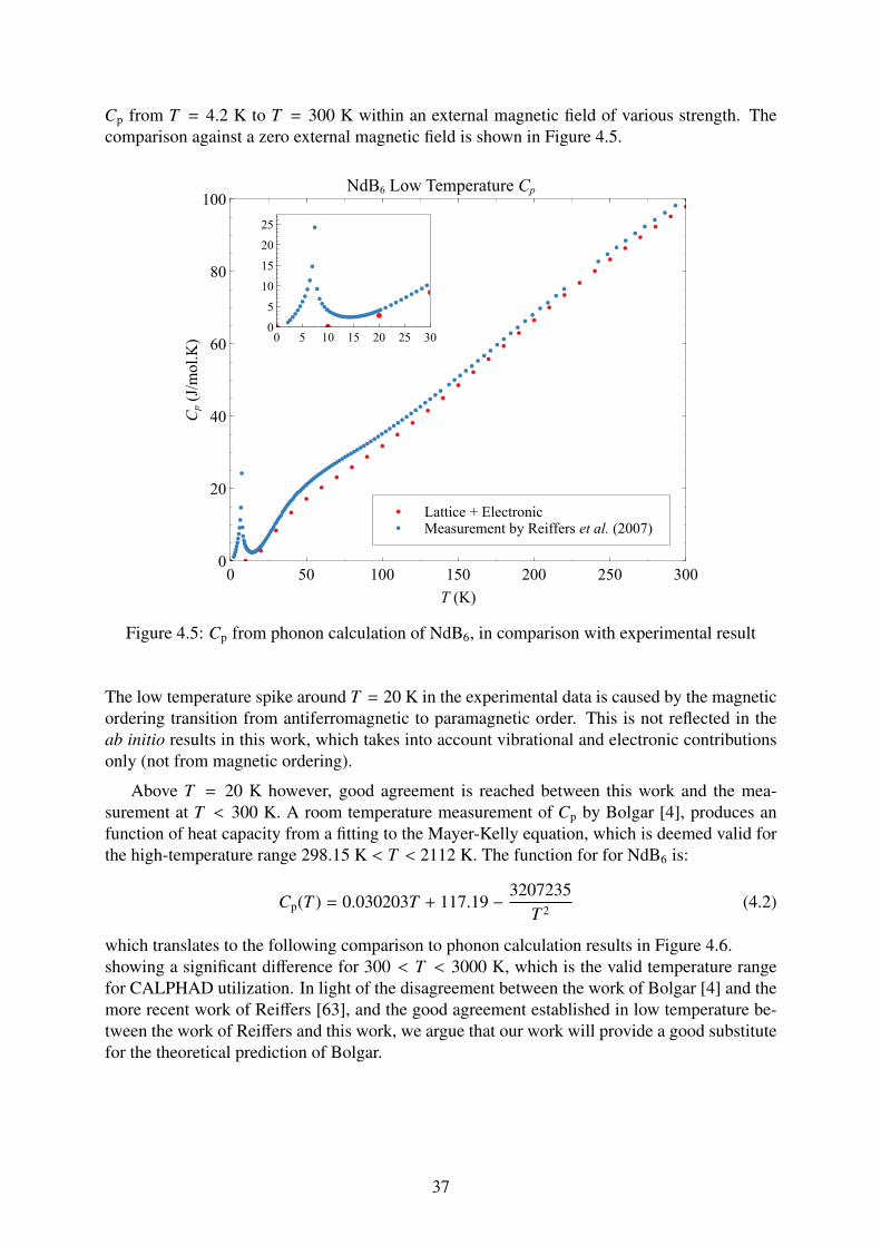
Cp from T = 4.2 K to T = 300 K within an external magnetic field of various strength. Thecomparison against a zero external magnetic field is shown in Figure 4.5.

0

5

10

15

20

25

0 5 10 15 20 25 30

Lattice+ElectronicMeasurementbyReiffersetal.(2007)

Cp(

J/m

ol.K

)

0

20

40

60

80

100

T(K)0 50 100 150 200 250 300

NdB6LowTemperatureCp

Figure 4.5: Cp from phonon calculation of NdB6, in comparison with experimental result

The low temperature spike around T = 20 K in the experimental data is caused by the magneticordering transition from antiferromagnetic to paramagnetic order. This is not reflected in theab initio results in this work, which takes into account vibrational and electronic contributionsonly (not from magnetic ordering).

Above T = 20 K however, good agreement is reached between this work and the mea-surement at T < 300 K. A room temperature measurement of Cp by Bolgar [4], produces anfunction of heat capacity from a fitting to the Mayer-Kelly equation, which is deemed valid forthe high-temperature range 298.15 K < T < 2112 K. The function for for NdB6 is:

Cp(T ) = 0.030203T + 117.19 − 3207235T 2 (4.2)

which translates to the following comparison to phonon calculation results in Figure 4.6.showing a significant difference for 300 < T < 3000 K, which is the valid temperature rangefor CALPHAD utilization. In light of the disagreement between the work of Bolgar [4] and themore recent work of Reiffers [63], and the good agreement established in low temperature be-tween the work of Reiffers and this work, we argue that our work will provide a good substitutefor the theoretical prediction of Bolgar.

37

Lattice+ElectronicLatticeElectronicEstimationbyBolgaretal.(1993)

Cp(J/mol.K)

0

50

100

150

200

250

T(K)0 500 1000 1500 2000 2500 3000

NdB6LatticeandElectronicContributiontoCp

Figure 4.6: Cp from phonon calculation of NdB6, in comparison with estimation from the workof Bolgar et al. [4]

4.2.2 NdB4

Figure 4.7: Unit cellof NdB4 phase

The NdB4 ground state crystal structure is a distorted structure fromthe simple cubic structures of NdB6. Both the Nd atom and octahe-dral B sublattices are distorted, introducing B atom pairs between thedistorted Nd sublattices, shown in Figure 4.7.

The initial atomic positions and lattice parameters are taken fromthe work of Salamakha et al. [75] on the single crystal X-ray diffrac-tion of NdB4. The ground state tetragonal crystal structure has thespace group P4/mbm, and the unit cell contains Z = 4 formula units.The initial lattice parameters are:

A: 7.1775 ÅB: 7.1775 ÅC: 4.0996 Å

These values do not significantly change after geometry optimization. As with NdB6, the sin-gle Hubbard site is determined to have a Ueff correction value of 5.7931 eV. The results of thecalculations are shown in Table 4.2.

GGA+U calculation values provides good agreement with the experimental work of Mescheland Kleppa [61] using direct synthesis calorimetry. The order of agreement with experimentaldata is comparable to that of the same result for NdB6. This result shows the validity of themethod used in this work to calculate the enthalpy of formation.

38

Phase Total Energy [Ry] Z x CalculationNdB4 -2333.49114589 4 1 -583.37278647Nd -2149.35042903 4 1 -537.33760726B -137.51578368 12 4 -45.83859456Eform [Ry] -0.19658465Eform, GGA+U [kJ/mol.atom] -51.61328937Expt. [kJ/mol.atom] [61] 53.3 ± 1.5Eform, GGA [kJ/mol.atom] -56.48200298

Table 4.2: NdB4 Formation Enthalpy

Watanuki et al. [76] performed Cp measurement for the very low temperature region, show-ing several successive magnetic ordering transitions at T = 4.8 K, T = 7.0 K, and T = 17.2K. These transitions lend credence to the hypothesis that NdB4 possesses multipolar magneticordering, a state recently confirmed in another study on NdB4. [64] Again, these transitions dueto electronic contribution are not reflected in the phonon calculation results.

As with NdB6, Bolgar et al. also fitted an enthalpy measurement with the Mayer-Kellyequation for 298.15 K < T < 2307 K. The equation for NdB4 reads:

Cp(T ) = 0.021044T + 116.55 − 4454762T 2 (4.3)

This function agrees well with the estimation of NdB4 heat capacity from an earlier work [77].

Lattice+electronicLatticeElectronicEstimationbyBolgaretal.(1993)

Cp(J/mol.K)

0

50

100

150

200

T(K)0 500 1000 1500 2000 2500 3000

NdB4constantpressurespecificheat(Cp)

Figure 4.8: Cp from phonon calculation of NdB4, in comparison with estimation from the workof Bolgar et al. [4]

Again, it shows a marked difference to the phonon calculation results for the high-temperatureregion, displayed in Figure 4.8. As with NdB6, the results of our work is chosen for CALPHADuse.

39

4.2.3 Nd2B5

Figure 4.9: Unit cell ofNd2B5 phase

The binary phase Nd2B5 ground state crystal structure pos-sesses the space group C2/c, with monoclinic crystal struc-ture, based on the prototype structure Pr2B5. From the basiccrystallographic data, a primitive cell was made and geometryoptimization was run, resulting in lattice parameters of:

A: 8.3670 Å α: 72.845◦

B: 8.3670 Å β: 107.155◦

C: 7.2841 Å γ: 128.635◦

containing Z = 4 formula units per cell.

There are 2 inequivalent Wyckoff positions inhabited by Nd atoms, referred to in Figure 4.9as Nd1 and Nd2. Effective Hubbard U correction Ueff parameter was self-consistently deter-mined per the methods outlined in Chapter 2.1.2, resulting in Ueff values of:

Nd1: 5.2099 eVNd2: 5.0492 eV

However, compared to other binary Nd-B compounds NdB6 and NdB4, experimental data onNd2B5 are relatively scarce. Only the enthalpy of formation information is readily available,from direct synthesis calorimetry by Meschel and Kleppa. [62] This value, along with first-principles GGA+U calculation, is shown in Table 4.3.

Phase Total Energy [Ry] Z x CalculationNd2B5 -4528.94730505 4 1 -1132.23682626Nd -2149.34493787 4 2 -1074.67246894B -137.51536897 12 5 -57.29807040Eform [Ry] -0.26628692Eform, GGA+U [kJ/mol.atom] -49.93829695Expt. [kJ/mol.atom] [62] -38.9 ± 1.9

Table 4.3: Nd2B5 Formation Enthalpy

The calculated formation enthalpy differs more than 10 kJ/mol.atom than the available ex-perimental results. This discrepancy suggests that GGA+U first-principles assessment of for-mation enthalpy is not reliable for Nd2B5 for the purposes of application in CALPHAD. Thisdiscrepancy is further discussed in Chapter 5.

To our knowledge, there are no experimental data available of Cp for Nd2B5. The results ofthe phonon calculation are displayed in Figure 4.10.As such, without any sort of comparison to test its validity, there can be no conclusive statementsmade about its reliability of this Cp calculation.

For CALPHAD application, it might be necessary to adjust its weight as input data to theoptimization results, both in the binary and ternary levels. The similar results have been ob-tained in the recent DFT calculations for the Nd-B binary system by Colinet and Tedenac [78],as well as for isostructural Gd2B5 investigated in the same work. This discrepancy between

40

Lattice+electronicLatticeElectronic

Cp(J/mol.K)

0

50

100

150

200

250

T(K)0 200 400 600 800

Nd2B5constantpressurespecificheat(Cp)

Figure 4.10: Cp from phonon calculation of Nd2B5

experimental and DFT results suggests a characteristic of the R2B5 structure which is not be-ing captured by either GGA or GGA+U calculations. As such, the CALPHAD optimization isperformed by classifying Nd2B5 enthalpy of formation and Cp as outlier data and zero weightis added in the optimization.

4.2.4 Nd2Fe17

Figure 4.11: Unit cell of Nd2Fe17

phase

As one of only two stable binary compounds in theNd-Fe system (the other being the relatively recentlydiscovered Nd5Fe17 [57]), Nd2Fe17 is highly impor-tant to model this binary system.. The ground statecrystal structure possesses the space group R-3m,with Th2Zn17 being the prototype crystal structure.As such, the crystal coordinates and Wyckoff posi-tions follow those of Th2Fe17, while the initial lat-tice parameters are taken from the work of Long etal. [79] The unit cell contains Z = 3 formula units.

From the initial parameters, a rhombohedralprimitive cell was found with Z = 1 formula unitinside. Geometry optimization produces lattice pa-rameters as follows:

A: 6.4733 Å α: 83.012◦

B: 6.4733 Å β: 83.012◦

41

C: 6.4733 Å γ: 83.012◦

from initial lattice parameters found in the work of Long et al. [79]

Nd occupies one Wyckoff position, while four other inequivalent positions are occupied byFe. Five Hubbard sites in total are within the simulation cell.

Nd1: 5.6000 eVFe2: 3.0130 eVFe3: 3.1539 eVFe4: 3.0244 eVFe5: 2.9752 eV

These values are used in the GGA+U calculations of formation energy. The calculation isoutlined in Table 4.4.

Phase Total Energy [Ry] Z x CalculationNd2Fe17 -6672.35190026 1 1 -6672.35190026Nd -2149.34082403 4 2 -1074.67041201Fe -329.27248982 1 17 -5597.63232694Eform [Ry] -0.18721116Eform, GGA+U [kJ/mol.atom] -3.39665762Expt. [kJ/mol.atom] [80] -3.0 ± 3.9

Table 4.4: Nd2Fe17 Formation Enthalpy

Phonon calculation results are displayed in Figure 4.12. The enthalpy of formation obtaineagrees relatively well with the available experimental measurement by Meschel and Kleppa [80].There is, however, little to no information regarding the experimentally measured Cp for Nd2Fe17.

4.3 Ternary phasesAs previously mentioned, three stable compounds so far have been discovered in the Nd-Fe-B ternary system, which are the vital T1 (Nd2Fe14B) phase, T2 (Nd1.1Fe4B4), and the T3(Nd5Fe2B6) phase. The T2 and T3 phases in particular present a challenge due to its relativelyscarce information available. Multiple metastable states have been proposed for this ternarysystem, and while modelling them may be relevant to investigate certain thermodynamic phe-nomena or phase transitions in the Nd-Fe-B ternary system, generally speaking the three stablephases should take priority in any assessment.

A similar equation is used to obtain the formation enthalpy from the ternary phase. As withEquation (4.1), it subtracts the total energies of the ground state unary phases from the ternaryphase. For the ternary phase AxByCz,

Eform = EAxByCz − xEA − yEB − zEC (4.4)

the molar fractions x, y, and z are collectively referred to as x. Each total energy is of oneformula unit Z = 1. The formation enthalpy obtained is converted to the units [kJ/mol.atom].

42

Lattice+electronicLatticeElectronic

Cp(

J/mol.K

)

0

100

200

300

400

500

600

700

T(K)0 500 1000 1500 2000 2500 3000

Nd2Fe17constantpressurespecificheat(Cp)

Figure 4.12: Cp from phonon calculation of Nd2Fe17

4.3.1 Nd5Fe2B6

Figure 4.13: Unit cellof Nd5Fe2B6 phase

The Nd5Fe2B6 or T3 phase has the ground state crystal structure ofthe space group R-3m, and as sucha rhombohedral primitive cellcan be constructed (with Z = 1). Initial ground state crystal struc-ture is taken from the work of Buschow et al. [81] and optimized,resulting in the following primitive cell:

A: 8.6834 Å α: 36.658◦

B: 8.6834 Å β: 36.658◦

C: 8.6834 Å γ: 36.658◦

This primitive cell is shown in Figure 4.13.

A total of 4 Hubbard sites are present in the cell, with 3 in-equivalent Nd atom positions and a single position occupied bythe Fe atoms.

Nd1: 5.6556 eVNd2: 5.3697 eVNd3: 5.3833 eVFe : 4.9680 eV

used in the GGA+U calculations for formation enthalpy. The for-mation enthalpy calculation is detailed in Table 4.5.

43

Phase Total Energy [Ry] Z x CalculationNd5Fe2B6 -3414.35007388 1 1 -3414.35007388Nd -2149.27878747 4 5 -2686.59848434Fe -329.27190272 1 2 -658.54380544B -137.51932421 12 6 -68.75966211Eform [Ry] -0.44812199Eform, GGA+U [kJ/mol.atom] -44.68669291

Table 4.5: Nd5Fe2B6 Formation Enthalpy

Lattice+electronicLatticeElectronic

Cp(

J/mol.K

)

0

100

200

300

400

500

600

T(K)0 500 1000 1500 2000 2500 3000

Nd5Fe2B6constantpressurespecificheat(Cp)

Figure 4.14: Cp from phonon calculation of Nd5Fe2B6

Phonon calculation results are displayed in Figure 4.14. Neither formation enthalpy norspecific heat measurements of this phase are available as comparison, and as such, care must betaken to weigh these data appropriately to well model the proper Nd-rich corner of the ternaryphase diagram.

4.4 CALPHAD assessmentCALPHAD assessment was performed for the binary Nd-B system using obtained thermody-namic data for compounds NdB4 and NdB6. The R-K polynomial coefficients were optimizedwith the PARROT module according to the enthalpy of formation and Cp theroetical predictionsdescribed in this chapter. The optimized Gibbs energy models give rise to the calculated phasediagram in Figure 4.16.

44

Cp/T(J/mol.K

2)

0

0.1

0.2

0.3

0.4

T(K)0 50 100 150 200

Figure 4.15: Calculated Cp/T plot for NdB6. An unusual peak is seen around T = 50 K,followed by the more expected linear section.

The results of the assessment of Chen et al. [53] which solely utilized available experimentaldata were used as a good starting point for the Gibbs energy parameters. These parameterswere further optimized, resulting in the displayed phase diagram, taking advantage of bothexperimental and ab initio results.

Several issues emerged during our re-optimization, most notably due to the Schottky-likeanomaly present in the Cp data for binary Nd-B compounds, seen in Figure 4.6 more detail inthe Cp/T plot in Figure 4.15 for NdB6. The Schottky anomaly is unlikely to be the cause of thisbroad peak, due to the cause of Schottky anomalies (entropy of spin populations in magneticmaterials) are unaccounted in the lattice vibrations. A similar anomaly can be seen for the caseof YB6 [82], however, which suggests that the same cause of the phenomena occurs in NdB6 aswell. In both materials there is large dependence of lattice volume on low temperature phononmodes, leading to the broad peak seen in Figure 4.15

This, coupled with the peak in Cp due to low temperature magnetic ordering shift, led to theimpossibility to fit the Cp data of either NdB6 and NdB4 for 0 < T < 3000 K, as is usually donewith specific heat measurements. Cp data of NdB6 fitted to a function from 300 < T < 3000K instead, and subsequently used to optimize directly the entropic term for the Gibbs energymodels for NdB6.

Our results do not differ much from that of our initial starting point for optimization fromChen et al. [53], with the significant exception for the area of the plot around NdB6 and NdB4, towhich we have applied the enthalpy of formation and Cp data from our calculation. Regardless,our results have shown that ab initio results from DFT+U can be used to optimize the Gibbsenergy models for the Nd-B binary system.

45

Nd2 B

5

NdB

4

NdB

6

NdB

66

1127.8

1279.0

2272.9

2880.6

2673.6

1388.0

2395.12348.0

T[K]

500

1000

1500

2000

2500

3000

X(Nd)0 0.2 0.4 0.6 0.8 1

Figure 4.16: Calculated phase diagram of the Nd-B binary system for T > 300 K, utilizing abinitio calculation results in this work

46

Chapter 5

Conclusion

Thermodynamic properties of some of Nd-Fe-B constituent phases have been obtained fromfirst-principles assessment in order to further CALPHAD assessment of the ternary system.Two thermodynamic properties are of interest for application in CALPHAD: the standard en-thalpy of formation and the specific heat under constant pressure or Cp. Enthalpy of formationwas obtained from DFT+U self-consistent calculations done with plane-wave basis set and theGGA-PBE exchange correlation functional. The effective Hubbard U correction is employedfor valence electrons in localized 3d and 4 f orbitals, and the parameter for this correction isdetermined self-consistently from first-principles [1].

Cp is obtained from phonon calculations of the constituent phases, using DFT as a atomicforce calculator from finite displacements of atomic sites (the frozen phonon approach). TheQuasi Harmonic Approximation (QHA) were employed over several values of unit cell vol-umes, leading to calculation of Cp. First-principle calculation methods are detailed in Chapter 2.

PhaseFormation Enthalpy [J/mol.atom]Eform Expt. data

NdB6 -45019 -46750 ± 1500NdB4 -51613 -53300 ± 1500Nd2B5 -49938 -38900 ± 1900Nd2Fe17 -3397 -3000 ± 3900Nd5Fe2B6 -44687 −

Table 5.1: Summary of formation enthalpies Eform obtained from first-principle calculations,with available experimental results for comparison

For both NdB6 and NdB4 binary phases, formation enthalpies were obtained with regularDFT (GGA-PBE) as well as the GGA+U correction. The Hubbard correction, in both cases,brought formation enthalpy values closer in agreement to experimental values, as shown inTables 4.1 and 4.2. While a marked improvement over non-corrected GGA is evident, theHubbard correction may not lead to better relative energetics for every compound. An exampleis an earlier work by Jain et al. [83] for the Fe-P-O phase diagram, in which neither GGAnor GGA+U alone correctly produces formation enthalpies. A mixing of the two results wasperformed which reduced the error significantly, but with the drawback of introducing empiricaldata to the method, limiting its predictive capability.

47

The differing values of Ueff used within the calculation of enthalpies of formation in thiswork stems from the application of the choice to use the linear response method of Cococcioniand de Gironcoli [1], which implies that different Ueff-values are appropriate for different com-pounds. While the conventional usage of the Hubbard U correction usually involves a uniform(equal) value of U term for traditional uses of DFT+U, adherence to the initial scheme seemsappropriate (accounting for the different chemical environments of each Hubbard site), espe-cially when the work of Jain et al. [83] supports mixing of energies with regular GGA (Ueff = 0eV).

GGA+U calculation results obtained in this work mostly correspond well with availableexperimental data. An exception appeared for the binary Nd2B5 phase, for which there is a 10kJ/mol.atom difference between the experimental determination of Meschel and Kleppa [62]using direct synthesis calorimetry and this calculation. The cause for the large discrepancy isnot conclusively determined. Previous works with GGA exchange correlation potential alsoshow this large discrepancy [78,84,85], and GGA+U method used in this work does not rectifythis discrepancy. Previous semi-empirical estimation of Nd2B5 with Miedema’s method hasalso failed to reach agreement with this measurement.

One interesting observation to bring up is that the discrepancy also exists for Gd2B5, whichpossesses the same crystal structure as Nd2B5. [78] The reason for the discrepancy seems tobe more related to the property of the crystal structure that is not captured by either GGA orGGA+U method. Another possibility is that the direct synthesis calorimetry used to measurethe enthalpy of formation for both compounds was inaccurate. However, this is consideredunlikely as the same work was used to establish the enthalpy of formation for NdB4 as well,which tracks very well with ab initio results. [62] As a result, specifically the ab initio results forNd2B5 were subsequently treated as outliers in the CALPHAD assessment, and thus weightedat zero in the Gibbs energy model optimization.

For the high-temperature regions, the estimation from the work of Bolgar et al. [4] disagreeswith the results of calculations for NdB6 and NdB4. This discrepancy, illustrated in Figures 4.6and 4.8, serves to highlight the improvements possible with ab initio methods over previous the-oretical approximations and assumptions. It should be noted that Bolgar’s estimation for NdB6

conflicts with measurement done by Reiffers it et al. [63], with which the phonon calculationresults presented in Chapter 4.2.1 achieves better agreement around T = 300 K.

Due to Cp peaks at lower temperature, the fitting of Cp data was not performed as it is usuallyperformed. Instead, the data from 300 < T < 3000 K is used as opposed to the fitting of lowtemperature data as well. The magnetic ordering shift, as well as the broad peak correspondingto anomaly also encountered in YB6, leads to difficulty in fitting the higher temperature regionto match the low temperature functions. In this way, the ab initio calculated thermodynamicdata of NdB6 and NdB4 by GGA+U method were successfully used in a reoptimization of theGibbs energy models for the binary Nd-B system, producing the reassessed phase diagram inFigure 4.16. This is the first time such ab initio calculation results have been successfully usedfor the Nd-B system CALPHAD reoptimization scheme.

48

Bibliography

[1] M. Cococcioni and S. de Gironcoli, “Linear response approach to the calculation of theeffective interaction parameters in the LDA+U method,” Phys. Rev. B, vol. 71, p. 035105,2005.

[2] M. A. van Ende and I. H. Jung, “Critical thermodynamic evaluation and optimization ofthe fe-b, fe-nd, b-nd, and nd-fe-b systems,” J. Alloys Compd., vol. 548, pp. 133–154, 2013.

[3] B. Hallemans, P. Wollants, and J. R. Roos, “Thermodynamic Assessment of the Fe-Nd-BPhase Diagram,” J. Phase Equib., vol. 16, pp. 137–149, 1995.

[4] A. S. Bolgar, V. B. Muratov, A. V. Blinder, A. I. Kryklya, and A. P. Suodis, “Thermody-namic properties of the rare earth borides and carbides in a wide temperature range,” J.Alloys Compd., vol. 201, pp. 127–128, 1993.

[5] H. L. Lukas, S. G. Fries, and B. Sundman, Computational Thermodynamics: The CalphadMethod. Cambridge University Press, 2007.

[6] M. Sagawa, S. Hirosawa, H. Yamamoto, S. Fujimura, and Y. Matsuura, “Nd-Fe-B Perma-nent Magnet Materials,” Jpn. H. Appl. Phys., vol. 26, p. 785, 1987.

[7] P. Tenaud, H. Lemaire, and F. Vial, “Recent improvements in NdFeB sintered magnets,”J. Magn. Magn. Mater., vol. 101, pp. 328–332, 1991.

[8] D. S. Sholl and J. A. Steckel, Density Functional Theory: A Practical Introduction. Wiley,2009.

[9] A. Jacob, C. Schmetterer, L. Singheiser, A. Gray-Weale, B. Hallstedt, and A. Watson,“Modeling of Fe-W phase diagram using first principles and phonons calculations,” Cal-phad, vol. 50, pp. 92–104, 2015.

[10] B. Hallemans, P. Wollants, and J. Roos, “Thermodynamic reassessment and calculation ofthe Fe-B phase diagram,” Zeitschrift fur metallkunde, vol. 85, pp. 676–682, 1994.

[11] T. V. Rompaey, K. C. H. Kumar, and P. Wollants, “Thermodynamic optimization of theB-Fe system,” J. Alloys Compd., vol. 334, pp. 173–181, 2002.

[12] K. Hongo, N. T. Cuong, and R. Maezono, “The Importance of Electron Correlation onStacking Interaction of Adenin-Thymine Base-Pair Step in B-DNA: A Quantum MonteCarlo Study,” J. Chem. Theory Comput., vol. 9, no. 2, pp. 1081–1086, 2013.

[13] K. S. Qin, T. Ichibha, K. Hongo, and R. Maezono, “Inconsistencies in ab initio evalu-ations of non-additive contributions of DNA stacking energies,” Chem. Phys., vol. 529,p. 110554, 2020.

49

[14] P. Hohenberg and W. Kohn, “Inhomogeneous Electron Gas,” Phys. Rev., vol. 136, no. 3B,pp. B864–B871, 1964.

[15] W. Kohn and L. J. Sham, “Self-Consistent Equations Including Exchange and CorrelationEffects,” Phys. Rev., vol. 140, no. 4A, pp. A1133–A1138, 1965.

[16] H. J. Monkhorst and J. D. Pack, “Special points for brillouin-zone integrations,” Phys.Rev. B, vol. 13, p. 5188, 1976.

[17] N. Marzari, D. Vanderbilt, A. D. Vita, and M. C. Payne, “Thermal contraction and disor-dering of the al(110) surface,” Phys. Rev. Lett., vol. 82, p. 3296, 1999.

[18] D. R. Hamann, M. Schluter, and C. Chiang, “Norm-conserving pseudopotentials,” Phys.Rev. Lett., vol. 43, pp. 1494–1497, 1979.

[19] L. Kleinman and D. M. Bylander, “Efficacious form for model pseudopotentials,” Phys.Rev. Lett., vol. 48, pp. 1425–1428, 1982.

[20] P. E. Blochl, “Projector augmented-wave method,” Phys. Rev. B, vol. 50, p. 17953, 1994.

[21] G. Kresse and D. Joubert, “From ultrasoft pseudopotentials to the projector augmented-wave method,” Phys. Rev. B, vol. 59, p. 1758, 1999.

[22] J. P. Perdew and A. Zunger, “Self-consistent equations including exchange and correlationeffects,” Phys. Rev. B, vol. 23, pp. 5048–5079, 1981.

[23] J. P. Perdew, K. Burke, and M. Ernzerhof, “Generalized gradient approximation madesimple,” Phys. Rev. Lett., vol. 77, p. 3865, 1996.

[24] S. L. Dudarev, G. A. Botton, S. Y. Savrasov, C. J. Humphreys, and A. P. Sutton, “Electron-energy-loss spectra and the structural stability of nickel oxide: An LSDA+U study,” Phys.Rev. B, vol. 57, pp. 1505–1509, 1998.

[25] M. Lazzeri, C. Attaccalite, L. Wirtz, and F. Mauri, “Impact of the electron-electron corre-lation on phonon dispersion: Failure of LDA and GGA DFT functionals in graphene andgraphite,” Phys. Rev. B, vol. 78, p. 081406(R), 2008.

[26] M. Sagawa, S. Hirosawa, H. Yamamoto, S. Fujimura, and Y. Matsuura, “Cu2ZnSnS4 as apotential photovoltaic material: A hybrid Hartree-Fock density functional theory study,”Jpn. H. Appl. Phys., vol. 26, p. 785, 1987.

[27] J. Hubbard, “Electron correlations in narrow energy bands,” Proc. Math. Phys., vol. 276,no. 1365, pp. 238–257, 1963.

[28] V. I. Anisimov, J. Zaanen, and O. K. Andersen, “Band theory and Mott insulators: Hub-bard U instead of Stoner I,” Phys. Rev. B, vol. 44, pp. 943–954, 1991.

[29] V. I. Anisimov, I. V. Solovyev, M. A. Korotin, M. T. Czyzyk, and G. A. Sawatzky,“Density-functional theory and NiO photoemission spectra,” Phys. Rev. B, vol. 48, no. 23,p. 16929, 1993.

[30] V. I. Anisimov, F. Aryasetiawan, and A. I. Lichtenstein, “First-principles calculations ofthe electronic structure and spectra of strongly correlated systems: the LDA+U method,”J. Phys. Condens. Matter, vol. 9, pp. 767–808, 1997.

50

[31] I. V. Solovyev and P. H. Dederichs, “Corrected atomic limit in the local-density approx-imation and the electronic structure of d impurities in Rb,” Phys. Rev. B, vol. 50, no. 23,p. 16861, 1994.

[32] A. I. Liechtenstein, V. I. Anisimov, and J. Zaanen, “Density-functional theory and stronginteractions: Orbital ordering in Mott-Hubbard insulators,” Phys. Rev. B, vol. 52, no. 8,p. R5467, 1995.

[33] O. Gunnarsson, O. K. Andersen, O. Jepsen, and J. Zaanen, “Density-functional calculationof the parameters in the Anderson model: Application to mn in CdTe,” Phys. Rev. B,vol. 39, no. 3, p. 1708, 1989.

[34] P. Giannozzi, S. Baroni, N. Bonini, M. Calandra, R. Car, C. Cavazzoni, D. Ceresoli, G. L.Chiarotti, M. Cococcioni, I. Dabo, A. D. Corso, S. Fabris, G. Fratesi, S. de Gironcoli,R. Gebauer, U. Gerstmann, C. Gougoussis, A. Kokalj, M. Lazzeri, L. Martin-Samos,N. Marzari, F. Mauri, R. Mazzarello, S. Paolini, A. Pasquarello, L. Paulatto, C. Sbraccia,S. Scandolo, G. Sclauzero, A. P. Seitsonen, A. Smogunov, P. Umari, and R. M. Wentz-covitch, “Quantum espresso: a modular and open-source software project for quantumsimulations of materials,” J. Phys. Condens. Matter, vol. 21, p. 395502, 2009.

[35] J. F. Janak, “Proof that ∂E/∂ni = ϵi in density-functional theory,” Phys. Rev. B, vol. 18,no. 12, p. 7165, 1978.

[36] P. H. Dederichs, S. Blugel, R. Zeller, and H. Akai, “Ground States of Constrained Systems:Application to Cerium Impurities,” Phys. Rev. Lett., vol. 53, no. 26, p. 2512, 1984.

[37] T. Yanai, G. I. Fann, Z. Gan, and R. J. Harrison, “Multiresolution quantum chemistry inmultiwavelet bases: Analytic derivatives for Hartree-Fock and density functional theory,”J. Chem. Phys., vol. 121, p. 2866, 2004.

[38] J. D. Head and M. C. Zerner, “A Broyden-Fletcher-Goldfarb-Shanno optimization proce-dure for molecular geometries,” Chem. Phys. Lett., vol. 122, pp. 264–270, 1985.

[39] A. Togo and I. Tanaka, “First principles phonon calculations in materials science,” Scr.Mater., vol. 108, pp. 1–5, 2015.

[40] G. Kresse and J. Hafner, “Ab initio molecular dynamics for liquid metals,” Phys. Rev. B,vol. 47, p. 558, 1993.

[41] G. Kresse and J. Hafner, “Ab initio molecular dynamics simulation of the liquid-metal-amorphous-semiconductor transition in germanium,” Phys. Rev. B, vol. 49, p. 14251, 1994.

[42] G. Kresse and J. Furthmuller, “Efficiency of ab initio total energy calculations for metalsand semiconductors using a plane-wave basis set,” Comput. Mat. Sci., vol. 6, p. 15, 1996.

[43] G. Kresse and J. Furthmuller, “Efficient iterative schemes for ab initio total-energy calcu-lations using a plane-wave basis set,” Phys. Rev. B, vol. 54, p. 11169, 1996.

[44] F. Birch, “Finite Elastic Strain of Cubic Crystals,” Phys. Rev., vol. 71, p. 809, 1947.

[45] L. Kaufman, “The lattice stability of metals - I. Titanium and zirconium,” Acta Metallur-gica, vol. 7, no. 8, pp. 575–587, 1959.

51

[46] J. O. Andersson, T. Helander, L. Hoglund, P. F. Shi, and B. Sundman, “Thermo-Calcand DICTRA, Computational tools for materials science,” Calphad, vol. 26, pp. 273–312,2002.

[47] A. Dinsdale, “SGTE Data for Pure Elements,” Calphad, vol. 15, pp. 317–425, 1991.

[48] J. Tomiska, “Mathematical conversions of the thermodynamic excess functions repre-sented by the Redlich-Kister expansion, and by the Chebyshev polynomial series to powerseries representations and vice-versa,” Calphad, vol. 8, pp. 283–294, 1984.

[49] K. Girgis, M. Kraft, U. Weis, P. Fischer, and M. Sostarich, “Crystal and magnetic structureof the permanent magnet materials Nd2Fe14−xCoxB (x = 0 − 14),” J. Less Common Met.,vol. 162, pp. 335–342, 1990.

[50] Y. Matsuura, S. Hirosawa, H. Yamamoto, S. Fujimura, M. Sagawa, and K. Osamura,“Phase diagram of the Nd-Fe-B ternary system,” Jpn. J. Appl. Phys., vol. 24, no. 8A,p. L635, 1985.

[51] V. Raghavan, “B-Fe-Nd (Boron-Iron-Neodymium),” J. Phase Equilib., vol. 24, no. 5,pp. 451–454, 2003.

[52] G. J. Zhou, Y. Luo, and Y. Zhou, “Thermodynamic reassessment of the Nd-Fe-B ternarysystem,” J. Electron. Mater., vol. 45, no. 1, pp. 418–425, 2016.

[53] T. L. Chen, J. Wang, C. P. Guo, C. R. Li, Z. M. Du, G. H. Rao, and H. Y. Zhou, “Thermo-dynamic description of the Nd-Fe-B ternary system,” Calphad, vol. 66, p. 101627, 2019.

[54] E. K. Storms, “Phase Relationship, Vaporization, and Thermodynamic Properties ofNeodymium Hexaboride,” J. Phys. Chem., vol. 85, pp. 1536–1540, 1981.

[55] K. Tanaka and T. Saito, “Phase equilibria in TiB2-reinforced high modulus steel,” J. PhaseEquilib., vol. 20, p. 207, 1999.

[56] M. G. Poletti and L. Battezzati, “Assessment of the ternary Fe-Si-B phase diagram,” Cal-phad, vol. 43, pp. 40–47, 2013.

[57] F. J. Landgraf, G. S. Schneider, V. Villas-Boas, and F. P. Missel, “Solidification andsolid state transformations in Fe Nd: A revised phase diagram,” J. Less Common Met-als, vol. 163, pp. 209–218, 1990.

[58] F. J. Landgraf, F. P. Missel, G. Knoch, B. Grieb, and E.-T. Henig, “Binary Fe-Ndmetastable phases in the solidification of Fe-Nd-B alloys,” J. Applied Phys., vol. 70,pp. 6107–6109, 1991.

[59] W. Zhang, G. Liu, and K. Han, “The Fe-Nd (Iron-Neodymium) System,” J. Phase Equilib.,vol. 13, pp. 645–648, 1992.

[60] R. E. Aune and S. Seetharaman, “Experimental studies of heat capacities of Nd2Fe17,Nd2Fe17N1.49, and Nd2Fe17N1.75 alloys in the temperature range 273-773 K,” High Tem-perature Materials and Processes (UK) (UK), vol. 17, pp. 299–311, 1998.

[61] S. V. Meschel and O. J. Kleppa, “Standard Enthalpies of Formation of Some Borides of Ce,Pr, Nd, and Gd by High-Temperature Reaction Calorimetry,” J. Alloys Compd., vol. 226,pp. 243–247, 1995.

52

[62] S. V. Meschel and O. J. Kleppa, “Thermochemistry of Alloys of Transition Metals andLanthanide Metals with Some IIIB and IVB Elements in the Periodic Table,” J. AlloysCompd., vol. 321, pp. 183–200, 2001.

[63] M. Reiffers, J. Sebek, E. Santava, N. Shitsevalova, S. Gabani, G. Pristas, and K. Flachbart,“Heat Capacity of NdB6,” J. Magn. Magn. Mater., vol. 310, pp. e595–e597, 2007.

[64] H. Yamauchi, N. Metoki, R. Watanuki, K. Suzuki, H. Fukazawa, S. Chi, and J. A.Fernandez-Baca, “Magnetic structure and quadrupolar order parameter driven by geomet-rical frustration effect in ndb4,” J. Phys. Soc. Japan, vol. 86, p. 044705, 2017.

[65] A. Nakaue, “Studies on the pressure-temperature phase diagram of nd, sm, gd, and dy,” J.Less Common Met., vol. 60, pp. 47–58, 1978.

[66] R. M. Moon, J. W. Cable, and W. C. Koehler, “Magnetic structure of neodymium,” J.Applied Phys., vol. 35, pp. 1041–1042, 1964.

[67] R. Kohlhaas, P. Donner, and N. Schmitz-Pranghe, “Uber die temperaturabhangigkeit dergitterparameter von eisen kobalt und nickel im bereich hoher temperaturen,” Z. Angew.Phys., vol. 23, p. 245, 1967.

[68] V. L. Moruzzi, J. F. Janak, and A. R. Williams, Calculated Electronic Properties of Metals.Pergamon Press, 1978.

[69] G. W. Fernando, R. E. Watson, M. Weinert, A. N. Kocharian, A. Ratnaweera, and K. Ten-nakone, “Magnetic moment of iron in metallic environments,” Phys. Rev. B, vol. 61, no. 1,p. 375, 2000.

[70] M. J. van Setten, M. A. Uijttewaal, G. A. de Wijs, and R. A. de Groot, “Thermodynamicstability of boron: The role of defects and zero point motion,” J. Am. Chem. Soc., vol. 129,pp. 2458–2465, 2007.

[71] S. Shang, Y. Wang, R. Arroyave, and Z. K. Liu, “Phase stability in α- and β-rhombohedralboron,” Phys. Rev. B, vol. 75, p. 092101, 2007.

[72] G. Will and B. Kiefer, “Electron deformation density in rhombohedral α-boron,” Z. Anorg.Allg. Chem., vol. 627, pp. 2100–2104, 2001.

[73] C. M. McCarthy and C. W. Tompson, “Magnetic structure of ndb6,” J. Phys. Chem. Solids,vol. 41, pp. 1319–1321, 1980.

[74] H. Han, “Density-functional theory study of the effect of pressure on the elastic propertiesof cab6,” Chin. Phys. B, vol. 22, p. 077101, 2013.

[75] P. Salamakha, A. P. Goncalves, O. Sologub, and M. Almeida, “Single crystal investigationof the binary ndb4 compound,” J. Alloys Compd., vol. 316, pp. L4–L6, 2001.

[76] R. Watanuki, T. Kobayashi, R. Noguchi, and K. Suzuki, “Possible multipolar transition inNdB4,” J. Phys. Conf. Ser., vol. 150, p. 042229, 2009.

[77] O. H. Krikorian, Estimation of Heat Capacities and Other Thermodynamic Properties ofRefractory Borides, vol. UCRL-51043. California Univ., Livermore, Lawrence RadiationLab., 1971.

53

[78] C. Colinet and J. C. Tedenac, “Enthalpies of formation of rare-earth borides from firstprinciples and comparison with experimental values,” Calphad, vol. 62, pp. 49–60, 2018.

[79] G. J. Long, G. K. Marasinghe, S. Mishra, O. A. Pringle, Z. Hu, W. B. Yelon, D. P. Middle-ton, K. H. J. Buschow, and F. Grandjean, “A magnetic, neutron diffraction, and mossbauerspectral study of the nd2fe17−xalx solid solutions,” J. Appl. Phys., vol. 76, p. 5383, 1994.

[80] S. V. Meschel, P. Nash, Q. N. Gao, J. C. Wang, and Y. Du, “The standard enthalpies offormation of some binary intermetallic compounds of lanthanide-iron systems by hightemperature direct synthesis calorimetry,” J. Alloys Compd., vol. 554, pp. 232–239, 2013.

[81] P. Deppe, M. Rosenberg, and K. H. J. Buschow, “A Mossbauer spectroscopy study ofNd5Fe2B6,” Solid state commun., vol. 64, pp. 1247–1251, 1987.

[82] R. Lortz, Y. Wang, U. Tutsch, S. Abe, C. Meingast, P. Popovich, W. Knafo, N. Shitseval-ova, Y. B. Paderno, and A. Junod, “Superconductivity mediated by a soft phonon mode:Specific heat, resistivity, thermal expansion, and magnetization of YB6,” Phys. Rev. B,vol. 73, p. 024512, 2006.

[83] A. Jain, G. Hautier, S. P. Ong, C. J. Moore, C. C. Fischer, K. A. Persson, and G. Ceder,“Formation enthalpies by mixing GGA and GGA+U calculations,” Phys. Rev. B, vol. 84,p. 045115, 2011.

[84] J. E. Saal, S. Kirklin, M. Aykol, B. Meredig, and C. Wolverton, “Materials Design andDiscovery with High-Throughput Density Functional Theory: The Open Quantum Mate-rials Database (OQMD),” JOM, vol. 65, pp. 1501–1509, 2013.

[85] S. Kirklin, J. E. Saal, B. Meredig, A. Thompson, J. W. Doak, M. Aykol, S. Ruhl, andC. Wolverton, “The Open Quantum Materials Database (OQMD): assessing the accuracyof DFT formation energies,” npj Comput. Mater., vol. 1, p. 15010, 2015.

54

Biography

Name Mr. Adie Tri Hanindriyo

Date of Birth 23 November 1992

Educational Attainment Master of Material Science: Japan Advanced Institute of Science and

Technology, Ishikawa, Japan, 2018

Bachelor of Engineering: Bandung Institute of Technology,

Bandung, Indonesia, 2015

Scholarship 2015-2018: Monbukagakusho (MEXT) Scholarship

Work Experiences

Publications

[1] A.T. Hanindriyo, T.B.M.Y.Y. Prawira, M.K. Agusta, R. Maezono, H.K. Dipojono, “Com-putational Design of Ni-Zn Based Catalyst for Direct Hydrazine Fuel Cell Catalyst usingDensity Functional Theory” Procedia Engineering, vol. 170, p. 148-153, 2017

[2] A.T. Hanindriyo, S. Sridar, K.C. Hari Kumar, K. Hongo, and R. Maezono, “Ab initiothermodynamic properties of certain compounds in Nd-Fe-B system” Comp. Mat. Sci.,vol. 180, p. 109696, 2020

[3] A. Hermawan, A.T. Hanindriyo, E.R. Ramadhan, Y. Asakura, T. Hasegawa, K. Hongo, M.Inada, R. Maezono, and S. Yin, “Octahedral morphology of NiO with (111) facet synthe-sized from the transformation of NiOHCl for the NOx detection and degradation: experi-ment and DFT calculation” Inorg. Chem. Front., vol. 7, p. 3431-3442, 2020

[4] T. Hasegawa, A. Shigee, Y. Nishiwaki, M. Nagasako, A.T. Hanindriyo, K. Hongo, R. Mae-zono, T. Ueda, and S. Yin, “New layered perovskite family built from [CeTa2O7]− layers:coloring mechanism from unique multi-transitions” Chem. Commun., vol. 56, p. 8591-8594, 2020

[5] A. Raghav, A.T. Hanindriyo, K. Utimula, M. Abbasnejad, R. Maezono, and E. Panda “In-trinsic electronic defect states of anatase using density functional theory” Comp. Mat. Sci.,vol. 184, p. 109925, 2020

55