1

SPACECRAFT NAVIGATION USING CELESTIAL GAMMA-RAY SOURCES

Chuck S. Hisamoto* and Suneel I. Sheikh†

As the future of space exploration endeavors progresses, spacecraft that are ca-

pable of autonomously determining their position and velocity will provide clear

navigation advances to mission operations. Thus, new techniques for determin-

ing spacecraft navigation solutions using celestial gamma-ray sources have been

developed. Most of these sources offer detectable, bright, high-energy events

that provide well-defined characteristics conducive to accurate time-alignment

among spatially separated spacecraft. Utilizing assemblages of photons from

distant gamma-ray bursts, relative range between two spacecraft can be accu-

rately computed along the direction to each burst’s source based upon the differ-

ence in arrival time of the burst emission at each spacecraft’s location. Correla-

tion methods used to time-align the high-energy burst profiles are provided. A

simulation of the newly devised navigation algorithms has been developed to as-

sess the system’s potential performance. Using predicted observation capabili-

ties for this system, the analysis demonstrates position uncertainties comparable

to the NASA Deep Space Network for deep space trajectories.

INTRODUCTION

For space vehicles venturing beyond Earth orbit into deep space, current navigation methods

require frequent interaction and communication with Earth stations, which can significantly in-

crease mission scheduling and operational costs. The NASA Deep Space Network (DSN) is the

primary provider of navigation and communication for the U.S. and its partnering nations on

deep-space missions.1, 2

DSN’s capability has achieved mission success throughout its over fifty

years of operation. However, as exploration initiatives increase and operational usage expands,

the DSN has the potential for over-subscription due to its many ongoing and future planned mis-

sions, and thus stands to benefit from supplemental navigation augmentation capabilities designed

to reduce DSN operations cost. In addition to improved operational support, expanded explora-

tion of our solar system beyond current day capabilities will require innovative, non-conventional

techniques for vehicle navigation. Very few existing systems can provide this additional service

while reducing DSN workload. Therefore, new methods are required that support the DSN sys-

tem by alleviating any operational interruptions and providing for increased operational autono-

my of deep space vehicles.

* Research Scientist, ASTER Labs, Inc., 155 East Owasso Lane, Shoreview, Minnesota 55126. † Chief Research Scientist, ASTER Labs, Inc., 155 East Owasso Lane, Shoreview, Minnesota 55126.

Copyright © 2013 by authors. Permission to publish granted to The American Astronautical Society.

AAS 13-444

2

To address the challenges of future DSN operation and enhance position accuracy for deep

space vehicles, a novel relative navigation technology for deep-space exploration using measure-

ments of celestial gamma-ray sources has been developed that incorporates existing designs of

autonomous navigation technologies and merges these with the developing science of high-

energy sensor components. This new technology for interplanetary self-navigation, referred to as

Gamma-ray source Localization-Induced Navigation and Timing, or GLINT, provides important

enhancements to planned exploration and discovery missions, specifically by increasing the

onboard navigation and guidance capabilities, thereby reducing operational risk.

A previous study of a navigation system based on variable celestial X-ray sources (0.1 – 20

keV), referred to as the X-ray Navigation and Autonomous Position Verification program, or

XNAV, has shown the capability to support DSN measurements for deep space missions.3-9

The

analysis of the unique and periodic nature of X-ray pulsar sources utilized in this past study pro-

vides a basis for the new GLINT navigation concept. XNAV relies on pulsars located at known

positions on the sky and a pulse-timing model of the expected arrival time of each pulse. The pe-

riodic nature of these pulsar sources provides a reliable signal that can be continually detected

and tracked. An XNAV range measurement is calculated using an observed pulse profile on a

spacecraft and the predicted pulse arrival time from each pulsar’s model. The observation time

required to produce each XNAV measurement depends on each pulsar’s unique characteristics

and the spacecraft’s detector qualities. Many X-ray pulsars are faint and require long observation

times to generate sufficient usable data.7

This new GLINT study extends the XNAV navigation concepts to celestial sources emitting

much higher energy photons (20 keV – 1 MeV). This paper details GLINT techniques to use -

ray photons from distant celestial gamma-ray bursts (GRB) to provide measurements supporting

the continual estimation of three-dimensional spacecraft position and velocity. Whereas XNAV

concepts can compute an absolute position of a spacecraft with respect to an inertial origin, the

overall GLINT concept measures the relative range of an observing vehicle with respect to a ref-

erence observer along the line-of-sight to a celestial source. This relative position is computed

using multiple relative range measurements based upon the difference in the arrival time of the

burst at each spacecraft’s location. These relative-range measurements can be computed any-

where in the solar system (and beyond), wherever a spacecraft and reference station can detect the

same burst and share their reception information. Although these bursting events are aperiodic,

happening only once per star, GRBs emanate from all directions of the sky with sufficient regu-

larity for navigation. GLINT-based navigation solutions can be continuously updated while on an

interplanetary cruise, or in orbit about a destination planetary body, including asteroids. As a rela-

tive navigation solution, GLINT is intended to complement the DSN infrastructure, and the even-

tual XNAV concepts.

A significant advantage supporting the GLINT implementation is that -ray detectors are cur-

rently incorporated on almost all deep space missions and science missions in Earth orbit as part

of their instrument package. These detectors support the science investigations of space radiation,

as well as evaluation of the composition of elements on planetary bodies. Several operating -ray

detection systems are continuing to actively collect GRB photon data, providing an on-going re-

source for GLINT analysis. While GRB sources are non-repeating and non-periodic due to their

cataclysmic nature, their flux intensities are much higher than most other high-energy celestial

sources, including X-ray pulsars studied previously.5, 6

They therefore yield higher signal-to-noise

and more well-defined morphological profile characteristics for burst time comparisons.

An initial study using past and current observed -ray mission data has demonstrated that the

relative navigation performance of hundreds of kilometer accuracy is readily available. However,

3

it will be shown that sub-km level positioning is expected to be achieved by the GLINT system

using future enhanced photon timing and processing algorithms.

CELESTIAL GAMMA-RAY SOURCES

Gamma-ray bursts are the most powerful explosions known in the universe.10

They are ex-

tremely luminous, with many orders of magnitude more energy output in a few seconds than our

Sun emits in a year. GRBs are theorized to be produced during the evolutionary end-stages of

single and binary star systems. This includes the unusually energetic supernova explosions (so-

called hypernovae), the merger of two neutron stars, or when a small star is consumed by a black

hole.11

GRBs have been detected approximately once per day by past and existing science missions,

although they are theorized to occur at a much higher rate due to the concept of beaming, in

which the emissions from a burst are focused into only 1/100th of the total sky.

12 Thousands of

GRBs have been detected since they were initially discovered in 1967 by the Vela satellites.13

GRB events are typically named and catalogued according to their detection date, in the format

GRBYYYYMMDDx, where x is an optional letter designation for cases in which multiple bursts

occur on a given day. These sources are typically detectable via their emissions in the tens of keV

to MeV, and often higher, photon energy bands. Figure 1 shows a rendering of a GRB after the

collapse and explosion of the star, at which time energy is jettisoned from the core of the burst.

Figure 1. An artistic rendition of a GRB and its components.

(Credit: Illustration: CXC/M.Weiss; Spectrum: NASA/CXC/N.Butler et al.)

GRB Source Classification and Characterization

GRBs are typically classified morphologically into a few distinct classes, based on temporal

and flux characteristics.14-17

Using the term T90 as the time over which the burst emits from 5% to

95% of its total photon counts, long bursts are those with T90 > 2 sec, and are thought to be relat-

ed to massive star collapse.17

Short bursts, likewise, exhibit a duration of T90 < 2 sec. Another

classification approach is fluence, S, which is the photon flux integrated over time. High fluence

4

bursts exhibit S > 1.6x10–4

erg/cm2/T90, whereas low fluence bursts are those with S < 1.6x10

–4

erg/cm2/T90. Most bursts exhibit some degree of a fast-rise and exponential-decay, referred to as

FRED, behavior.

Short bursts are known to have harder spectra than long bursts, where a greater proportion of

the detected photons are of higher energy.19

The importance of spectral properties, coupled with

the sensitive energy band, E, of a given detector, can be seen in the relative statistics of GRB de-

tection between instruments and missions. For example, the Fermi spacecraft’s Gamma-ray Burst

Monitor (GBM), with an effective area a factor of ~3 smaller than that of Swift’s Burst Alert Tel-

escope (BAT), detects 1.5 times more GRBs per year.20

The reason for this dramatic difference is,

in part, GBM’s greater sky coverage, but also that GBM’s sensitivity extends over a much broad-

er energy band (8 keV ≤ E ≤ 30 MeV) than does BAT (15 keV ≤ E ≤ 150 keV). Because the

GBM’s higher-energy response is a better match to the hard-spectrum emission from short bursts,

a significantly larger fraction of bursts detected by GBM are short, compared to BAT. Because

short bursts tend to contain narrower temporal features that are better suited to high-precision

time of arrival comparison, the hard-spectrum nature of these types of bursts may dictate future

GLINT detector design decisions for optimized performance. Figure 2 provides six unique GRB

profiles recorded by various detector missions, which illustrate the diversity of burst characteris-

tics. In each subplot, the red and blue signals represent the incoming fluxes as received by the

respective spacecraft’s detector. Differences in flux magnitude between two observing spacecraft,

which can vary dramatically as shown, are due to the different detector properties on each space-

craft.

Figure 2. Sample of burst profiles for selected GLINT-processed GRBs.

Gamma-ray Pulsar Sources

The gamma-ray emissions of nearby neutron stars are visible as their radiation beams are

swept across the Earth’s line of sight by the stars’ rotations. Both young neutron stars — with

spin periods of tens of milliseconds and magnetic field strengths of order 1012

G — and those that

have been recycled in a past mass-accretion evolutionary episode, leaving them with spin periods

5

less than 10 ms and 109 G magnetic fields, are visible as sources of pulsed gamma rays; the latter

exhibit highly predictable timing behavior, enabling applications that rely on the regularity of

their pulsations.

Catalogues of rotation-powered pulsars from which pulsed -rays have been detected from the

Fermi and INTEGRAL missions detail basic properties and -ray fluxes that drive exposure times

required for useful navigation precision. The catalogue includes both rotation-powered pulsars

and soft-gamma repeaters (SGRs), which are bright, flaring, recurring sources.

The Fermi team has reported, in its published Second Source Catalog, 83 rotation-powered

pulsars from which pulsed -rays have been detected.21

(Another 25 known — from radio or X-

ray observations — pulsars are detected in -rays but without apparent pulsations.) Among the

pulsed sources, fluxes are typically at the level of 10-8

photons/cm2/sec; the brightest, the Vela

pulsar, has a flux of 3.4x10-6

photons/cm2/sec. These fluxes are integrated over the energy band

0.3 MeV to 1 GeV, where the (hard) -ray emissions of rotation-powered pulsars are brightest —

below a hundred MeV, Galactic background emission reduces signal-to-noise ratios considerably;

above a few GeV, pulsar spectra cut off exponentially.

The Fermi LAT's effective collecting area in the 0.3 – 1 GeV band is approximately 6,000

cm2, so that for the Vela pulsar, the detected photon flux is 0.02 counts/sec. While this flux level

is potentially conducive to navigation analysis in the manner of XNAV, scaling the large sized

LAT to a detector size that would be appropriate to a navigation subsystem would significantly

reduce the photon detection rate. Also, for a more-typical fainter -ray pulsar, the photon flux is

two orders of magnitude lower.

In the energy band at the low end of GRB emissions (tens to 100 keV), the INTEGRAL satel-

lite provides a good measure of typical fluxes for both rotation-powered pulsars and so-called

magnetars (SGRs and anomalous X-ray pulsars that are believed to be powered by the slow de-

cay of their enormously strong magnetic fields). In its survey mode, INTEGRAL detected three

pulsars, two AXPs, and two SGRs; these are among the brightest in their classes (pointed, non-

survey INTEGRAL observations are much more sensitive to dimmer sources). Typical fluxes in

both the soft (20 – 40 keV) and hard (40 – 100 keV) INTEGRAL bands for these seven objects are

in the vicinity of 3x10-4

ph/cm2/sec and with INTEGRAL's effective area of 2,600 cm

2 a detected

photon flux of ~1 count/sec is produced.

These detected INTEGRAL fluxes are for sources in their quiescent state. Rotation-powered

pulsars are not variable in flux, but both magnetar varieties exhibit sporadic, unpredictable flares;

those from SGRs can be exceedingly bright. These SGR flares are believed to recur every few

years. AXP flares, on the other hand, increase the quiescent flux by a factor of a 2 – 5, and recur

every few days-to-weeks, with larger flares being less frequent.

These low photon flux rates make the use of -ray pulsars an extreme challenge for a practical

navigation system.7 Thus, the more useful -ray sources are those of the high-flux GRB type.

THE INTERPLANETARY NETWORK AND GAMMA-RAY BURST COORDINATES

NETWORK

A significant infrastructure has been built to observe GRBs and rapidly disseminate infor-

mation about their occurrence and localizations. The Interplanetary Network (IPN), in existence

for over 30 years, comprises an inhomogeneous collection of in-space monitoring platforms that

triangulate the position of a GRB from the burst arrival time differences between spacecraft.22

This source localization service by IPN spacecraft provides an architecture for GRB timing and

positioning.

6

The Gamma-ray Burst Coordinates Network (GCN), established by NASA’s Goddard Space

Flight Center (GSFC), gathers input from IPN and optical and radio ground stations to dissemi-

nate the position of a GRB to observers as quickly as possible, sometimes less than a minute after

detection. The composition of the IPN and GCN supporting spacecraft and Earth observation sys-

tems are shown in Figure 3. This existing GRB observational infrastructure provides a prelimi-

nary basis for the architecture of the operational GLINT system. The network of IPN vehicles,

many with ongoing and extended missions, along with future planned missions already being

equipped with -ray detectors capable of high-accuracy timing, ensures the data availability that

feeds the GLINT concept.

Figure 3. The integrated GCN and spacecraft-based IPN architecture.

Historically, detections by many geometrically well-displaced observers of the afterglow of a

GRB subsequent to its detection have provided localization of the GRB on the sky. The known

position of each observer assisted with the localization. Today, the Swift mission, with its GRB

detector plane area of ~5200 cm2, localizes GRBs at the arcsecond level, and ground- or space-

based follow-up in the optical or radio bands can localize afterglows to significantly better than

an arcsecond of accuracy.

GLINT NAVIGATION SYSTEM ARCHITECTURE

This multi-spacecraft localization process, as part of the GCN and IPN, improves the analysis

of these one-time celestial GRB events. In principle, however, the IPN procedure can be inverted

to improve or determine independently the position of any spacecraft that detects a GRB that has

been well localized by Swift or ground-based follow-up. This is the basic concept of GLINT de-

tailed in Figure 4. This diagram shows the primary elements of a notional GLINT system archi-

tecture, which includes a base observational reference station orbiting Earth, and a remote space

vehicle. Both the base and remote spacecraft are shown detecting the same GRB event. Earth

ground station data processing is used to support the rapid dissemination of GRB data products

among cooperating vehicles.

The operation of a GLINT GRB base and remote spacecraft based range measurement pro-

ceeds as follows. High-resolution binning detectors on-board the base and remote spacecraft

7

would accumulate a light curve for the duration of the -ray burst using fine-resolution time-

tagged photon arrival times to ensure precise and accurate observations. The accurate line of sight

to a GRB, , is disseminated by the IPN/GCN system once the GRB has been precisely localized.

To provide the required GRB localization accuracy, the GLINT base station would require Swift-

like arcsecond localization capabilities, or an optical follow-up (ground or space). The GLINT-

equipped remote spacecraft would use the base station template light curve profiles and its own

observed data, along with the known accurate sky position disseminated by the IPN/GCN, to

compute the time difference of arrival (TDOA) of the burst between spacecraft. Using this meas-

ured burst TDOA, the remote spacecraft would compute its position relative to the base station

and a navigation solution incorporating this measured relative distance would be updated, provid-

ing a refined navigation solution.

Figure 4. The GLINT concept and architecture for spacecraft navigation.

Two potential data transmission and processing paths are available for GLINT. In one ap-

proach, the processing of the TDOA between the acquired light curves and the relative navigation

solution, including any cross correlation and filtering techniques, would be performed on-board

the GLINT-equipped spacecraft and the navigation solution would be updated. Thus, the data te-

lemetry path is up to the remote spacecraft, where the remote vehicle itself computes and updates

its own navigation solution. In another approach, the light curves obtained by each observing

spacecraft would be telemetered down to a central ground- or space-based processing station. The

cross-correlation between light curves and navigation solution refinement would be performed at

this central station. The updated navigation solution based on the relative distances would then be

maintained at the central station and future control maneuvers could be planned accordingly.

GAMMA-RAY BURST PHOTON DATA PROCESSING

Observational data of a GRB primarily include the time of the detected event, its location, and

a table of photon count data over a specified time interval. These light curve data files provide the

8

shape and intensity of a single GRB. Among the primary components of the light curve files

found in public databases or obtained by permission of the mission scientists are a trigger time,

which specifies a starting time, t0, for the emission event, individual bin time stamps, and total

photon counts in each time bin. This data set can be compared between mutually observing

spacecraft to improve knowledge of the relative positions of the spacecraft by correlating the dif-

ference of the time of arrival between detections. From Figure 4, it is seen that the time offset, ,

of the burst arrival time at two spacecraft is related to their position offset, , along the unit line

of sight to the GRB, , as the following, where superscript T denotes the vector transpose,

(1)

In order to simulate the GLINT processing techniques, GRB light curve data containing as-

semblages of time-tagged photons were acquired from representative missions. As time-tagging

of incoming photons is performed with respect to mission-specific timescales, burst data were

first time-standardized to seconds-of-day UT1. An example burst, GRB20110420A as observed

by Swift and WIND, is shown in Figure 5. This burst featured a fast rise in photon counts, as seen

in the Swift/BAT light curve, displayed in red. The WIND observed profile, shown in blue, pro-

duced a corresponding energetic spike 1.863 seconds later, according to the difference in times of

the profile peaks. Close inspection of the profile observed by WIND shows the corresponding

spike to be the offset feature rather than the decreasing relative maximum at the start of the WIND

data. Differences in the magnitude of flux between the peaks observed by Swift and WIND are

due to differences in detector energy ranges. This TDOA measurement between profiles repre-

sents the delay of the arrival of the burst between the Swift and WIND vehicles, as Swift is in a

high Earth orbit, and WIND is at the Earth-Sun L1 Lagrange point. Based upon the known space-

craft locations at the detection times of this burst’s peak, the measured geometry-based offset

along the line of sight to the burst is 1.947 seconds. The difference between the known geomet-

rical offset and the TDOA measurement is therefore 84 ms. Using Eq. (1) this geometrical-based

time offset versus observed time offset discrepancy yields a position uncertainty of greater than

20000 km. However, the limitation of the burst profile’s bin size of 64 ms for both Swift and

WIND largely contributes to this computed uncertainty (~2 bins). Moreover, even with this poten-

tially large uncertainty, this simple example based upon peak arrival time of binned photon data

effectively demonstrates the GLINT concept. To extend this GLINT concept to improved capa-

bilities, refined cross-correlation methods with the ability to attain time uncertainties less than

1 ms with existing GRB observation data are further described below.

Figure 5. GRB20110420A, a FRED-type burst yielding accurate TDOA values.

9

METHODS OF GAMMA-RAY BURST COMPARISON

To support the evaluation of existing GRB data for TDOA measurements in navigation, mul-

tiple methods of comparing and time-aligning GRB light curves have been devised. These meth-

ods, described in further detail below, include a maximum burst peak alignment, a MATLAB

cross-correlation function, and a Fourier-domain burst phase alignment.

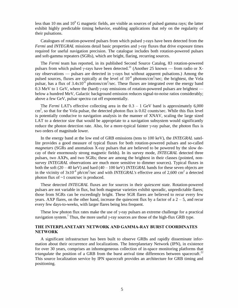
A GLINT burst TDOA analysis tool was created to process binned light curve data from mul-

tiple sets of two specified spacecraft. Once time-standardized light curves from the pre-processed

photon data are generated, an Earth-Centered Inertial (ECI) line-of-sight (LOS) is calculated for

the detected GRB event to the spacecraft using its right ascension and declination values provided

by GCN’s burst alert notices. In order to validate the TDOA value between spacecraft for each

burst, the tool referenced the spacecraft position at the time of peak emission. To do this, it read

in the spacecraft ephemeris data and located the spacecraft position at the peak time in the light

curve, using a piecewise cubic hermite interpolation of spacecraft ephemeris data to find the posi-

tion at the time of peak emission during the burst. Figure 6 shows the GRB pulse alignment from

two observing vehicles, first by aligning the pulse peak according to the detector trigger time,

noted in the GCN alerts, and then by a second-of-day timing, according to the actual photon-

measured arrival time at the vehicle.

Figure 6. Comparisons using two GRB instruments for GRB080727B, using trigger time (top panel)

and second-of-day (bottom panel).

10

Maximum Burst Peak Alignment

A simple burst comparison method utilized, as illustrated for GRB20110420A in Figure 5,

compares the burst peak arrival times. The light curve profiles for a selected burst, as seen by two

or more spacecraft are overlaid according to their binned, time-stamped data. The exact second-

of-day time of the observed maximum intensity value corresponding to the burst peak are record-

ed. The TDOA measurement is the difference of these burst peak times between vehicles. Broad-

er GRBs that lack the fast rise burst in Figure 6 are not as easily compared by peak alignment.

However, the rapid increase in flux at the initial burst emission lends itself to the multiple sharp

maxima for this burst, resulting in accurate TDOA determination.

Burst Profile Cross-Correlation

To improve upon the performance of the GRB profile time alignment and utilize all the burst’s

photon data, TDOA determinations for the GRBs using a cross-correlation of the light curves was

accomplished using MATLAB’s xcorr. This function uses two burst profiles as input, and its out-

put of the cross-correlation lags indicate the individual bin offset between burst profiles.

Fast Fourier Transform Fitting

A Fourier domain cross correlation analysis of GRB profiles was accomplished using the Fast

Fourier Transform Fit (FFTFIT) algorithm,23

to produce a more refined TDOA result than the two

techniques above. This FFTFIT technique and software tool has been previously developed for

radio and X-ray pulsar timing analysis; a recent implementation is part of the overall PSRCHIVE

software package.24

This tool estimates fractions of a bin offset, or lags, between two light curves

without attempting to derive an arrival time of the peak for each. As FFTFIT resolves TDOA lags

as a small fraction of a time bin, for bursts that have desired profile characteristics for good pro-

cessing candidacy, TDOA resolutions are improved using FFTFIT over both peak alignment and

cross correlation methods described above. Many of the TDOA lags computed by FFTFIT were

on the order of a hundredth of a bin, yielding accuracies less than a millisecond using bin sizes

for analyzed observations ranging from 32 to 64 ms. The benefit of the FFTFIT processing tool is

the ability to correlate bursts with broader morphological profiles than the previous two methods.

GRB Time Offset Computation Results

Data from existing spacecraft and instruments were investigated, including both Earth-orbiting

and deep space vehicles. These instruments included the BAT onboard Swift, Konus onboard

WIND, the Anti-Coincidence Shield of the Spectrometer onboard INTEGRAL (SPI-ACS), the

Wide Area Monitor (WAM) of Suzaku, MESSENGER’s Gamma-Ray Neutron Spectrometer

(GRNS), and Mars Odyssey’s High Energy Neutron Detector (HEND). Photon fluxes measured

by the instruments onboard most spacecraft have been stored in timed bins, with the bin size

varying between instruments. TDOA measurements demonstrated agreement between multiple

methods including maximum burst peak, burst cross-correlation, and FFTFIT. The measured

TDOA from each method and the actual known vehicle geometry-based time offset were com-

pared to compute the number of bins of accuracy achievable.

Most GRB events, including GRB20080727B shown in Figure 6, featured distinct periods of

emission, which could be easily correlated with the corresponding energetic spike seen by another

spacecraft for which methods such as maximum burst peak can work well. Precise TDOA calcu-

lations for bursts displaying chaotic and noisy structures, for instance, GRB20080319B, are more

difficult to achieve using the maximum burst peak method, lacking well-defined features to iso-

late. The same holds true for bursts exhibiting plateau profiles with long and broad features on

the time axis.

11

The maximum burst peak-based analysis provides a basic approach for comparing GRB

TDOAs. However, this simplified technique only analyzes the time of the maximum photon

count values, not effectively utilizing all known data present within each burst. Analytically

cross-correlating using the other two methods, the two burst profiles provide improved solutions.

Using the known spacecraft geometry, an analysis of the xcorr cross-correlation technique in-

dicates equally good or better results as the maximum burst peak method. In many cases where

the burst does indeed display morphologies of sharp peaks or distinct, well-separated features

(e.g., GRB20080727B) the peak time alignment method results are slightly better than cross-

correlation, as the latter method attempts to align the entire temporal profile of the burst, much of

which can contain noise that distorts the light curve. However, in cases where the GRB profile

lacks a defined feature like a sharp peak (e.g., GRB20080319B) cross correlation using xcorr of

the light curves yields an improved TDOA, with uncertainties of two time bins or less. Accurate

alignment using peak time estimates is ineffective using these types of bursts, as their profiles can

be too broad and chaotic for isolating and windowing individual time-specific features.

For a preliminary GLINT concept analysis, several dozen representative GRB-spacecraft pair-

ings were analyzed using the above three TDOA comparison techniques. All bin offsets for pro-

cessed TDOA calculations were within four bins of accuracy, with many measurements within a

fraction of a bin of precision representing uncertainties of 1 ms or less. As anticipated, bursts with

sharp, energetic peaks and short durations are found to yield the most accurate TDOA compari-

sons. A small sample of nine processed bursts is provided in Table 1.

Limitations on TDOA bin resolution have been shown to depend largely on current photon da-

ta formats and binning sizes. Most GRB detector mission bin sizes are between 32 and 64 ms.

Through advances in timing capabilities, this bin timing is expected to be capable of improve-

ment to 1 ms-bins. The Konus instrument onboard WIND is currently capable of 2 ms bin resolu-

tion for some triggered bursts.25

Further advancement is likely, with the recent progress of tech-

nologies such as the JPL Deep Space Atomic Clock (DSAC), capable of sub-ns time uncertain-

ties.26

Current GLINT processing using FFTFIT has achieved 1/100th of a bin uncertainty ranges.

For enhanced performance, GLINT would require planned improvements to data processing

techniques and significantly enhanced -ray detector timing capabilities to achieve binning of less

than 100 μs, such that 1 μs or less burst TDOA uncertainties would be achievable.

Table 1. GLINT Timing Resolution Capabilities.

GRB

Identifier

Spacecraft

Observer

#1*

Spacecraft

Observer

#2*

Max Peak

Alignment

Resolution

[# Bins]

Burst

Profile Cross

Correlation

Resolution

[# Bins]

FFTFIT

Resolu-

tion

[# Bins]

FFTFIT

Uncer-

tainty

[#Bins]

20100625A Sw I 0.516 0.828 0.036 ---------

20100625A Sz W 0.297 0.078 --------- ---------

20100625A Sz I 0.719 0.688 0.103 ---------

20101219A W Sw 0.188 0.188 0.188 0.052

20111113A W I 2 2 0.094 0.020

20111121A Sz Sw 0.047 ---------** --------- ---------

20111121A W Sw 0.266 0.266 0.209 0.036

20111121A W Sz 0.047 0.047 --------- ---------

20120324 W Sw 0.641 2 0.986 0.191

*Sw = Swift/BAT; Sz = Suzaku/WAM; W = WIND/Konus; I = INTEGRAL/SPI-ACS

**Calculation not possible due to issues stated in text

12

GLINT NAVIGATION ALGORITHMS

In order to evaluate the performance of the designed GLINT concept, two navigation algo-

rithm methods were devised that use GRB TDOA measurements as input. The first approach pro-

duces a single scalar value that is computed using the TDOA measurement to formulate range

between vehicles along the line of sight to the GRB, as in Eq. (1). The second approach formu-

lates a full three-axis relative position measurement based upon Eq. (1), and is expected to pro-

vide an improved approach over the scalar method.

The primary function of the GLINT navigation system is to determine the accurate, full, three-

dimensional position, expressed as S {rx,ry,rz} , and velocity of the remote spacecraft.

These navigation states can be with respect to an inertial origin or expressed relative to a base, or

reference, spacecraft located at ase. The position separation, or difference, , between these

vehicles is computed as

1 S ase (2)

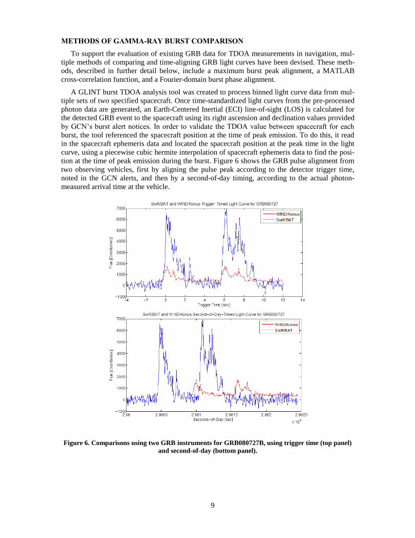
The diagram in Figure 7 shows this relationship and how the time offset relates to the position

separation expressed in Eq. (2). The primary measurement of the GLINT navigation system is the

time offset of the GRB arrival between two spatially separated spacecraft. The time offset, , is

computed as accurately as possible by any of the GRB comparison methods described above.

Figure 7. Observations of GRB event by GLINT base station and remote spacecraft.

To provide optimal GLINT data processing, the observations of the GRB time offsets can be

processed with an extended Kalman filter (EKF).27

The GLINT EKF uses the high fidelity orbit

dynamics of a vehicle, processes measurements, and updates the error solution and covariances.

Between burst measurements, the motion of the vehicles is incrementally propagated forward.

The EKF designed for GLINT uses the filter states of the error of position and velocity of the re-

mote vehicle. Error estimates of spacecraft clock synchronization, GRB direction, and planetary

ephemeris could be included as state variables in future implementations of the GLINT EKF.

The navigation states of the GLINT navigation system and EKF follow the methods previous-

ly developed for the XNAV system.4, 6, 8

The EKF states, , are vehicle position, , and velocity,

, as [ ] . The non-linear spacecraft orbital dynamics can be expressed as

(t) ( ), ) ) (3)

13

In Eq. (3) is the non-linear state vector function, as ( ( ), ) [ ] [ ] where is

the vehicle acceleration. The second term in Eq. (3), ), is the noise vector associated with the

unmodeled state dynamics. Using the dynamic models of acceleration of the spacecraft, including

the primary orbiting body gravitational effects and higher order disturbances, the full vehicle state

dynamics can be expressed.6

The GLINT Kalman filter is an extended Kalman filter due to the non-linear dynamics of the

orbiting spacecraft. The states of the GLINT EKF are the errors of the state vector. These error-

states, , can be represented based upon the true states, , and the estimated states, , as,

(4)

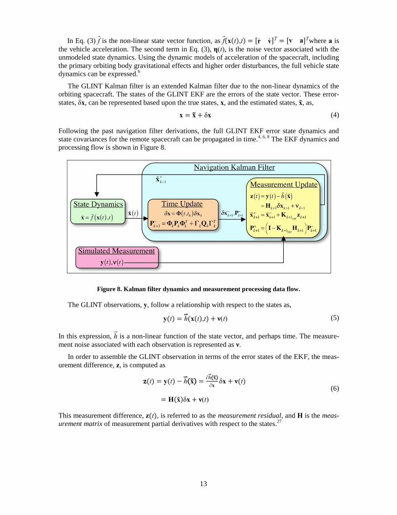
Following the past navigation filter derivations, the full GLINT EKF error state dynamics and

state covariances for the remote spacecraft can be propagated in time.4, 6, 8

The EKF dynamics and

processing flow is shown in Figure 8.

Figure 8. Kalman filter dynamics and measurement processing data flow.

The GLINT observations, , follow a relationship with respect to the states as,

( ) ( ( ), ) ) (5)

In this expression, is a non-linear function of the state vector, and perhaps time. The measure-

ment noise associated with each observation is represented as .

In order to assemble the GLINT observation in terms of the error states of the EKF, the meas-

urement difference, , is computed as

( ) ( ) ( ) ( )

( )

( ) )

(6)

This measurement difference, ( ), is referred to as the measurement residual, and is the meas-

urement matrix of measurement partial derivatives with respect to the states.27

14

Based upon the diagram of Figure 7, a scalar measurement implementation follows from the

range calculation using the observed GRB time offset as,

( )

[ ] ( ) (7)

This scalar method is straightforward to calculate from the GRB time offset, t and the esti-

mated remote spacecraft position and known base spacecraft position, r. Any discrepancy com-

puted in z is related to the errors in the remote spacecraft position and velocity using Eq. (7). The

range measurement is a singular scalar value and can only adjust a portion of the estimated vehi-

cle position and velocity with each GRB observation.

A second measurement approach uses a full three-dimensional approach in order to correctly

adjust all three axes of position and velocity with each GRB observation. This vector measure-

ment method is devised as,

) ( ) ( )

[( ) ( ) ( ) ] )

(8)

where i, j, k{ }are the unit axis directions for the spacecraft’s coordinate system.

Both the scalar and vector methods for GLINT EKF measurements were evaluated and, as ex-

pected, it was determined that the vector method provided improved processing and performance

with its multi-axis observation per measurement.

GLINT NAVIGATION SIMULATION AND PERFORMANCE

A simulation, written in MATLAB, was developed to evaluate the performance of the GLINT

navigation algorithms. The simulation propagates a truth model of a spacecraft on an interplane-

tary trajectory, and compares a similar trajectory initially injected with position and velocity er-

rors that is continually corrected by GLINT measurements. The comparison of the truth trajectory

with the corrected simulation provides an evaluation of EKF performance.

To evaluate the benefits of the GLINT navigation system, comparisons to DSN navigation so-

lutions were produced. This approach is similar to past research on the evaluation of navigation

using X-ray pulsars.8 A simulated heliocentric trajectory was chosen as 100 days prior to a ren-

dezvous at Mars, which was implemented based upon available trajectory data for the Mars Sci-

ence Laboratory (MSL) vehicle. (For a comparison of detector size, MSL’s Radiation Assessment

Detector (RAD) weighs 1.56 kg and is roughly 240 cm3 in volume.

28) The Earth to Mars inter-

planetary trajectory simulation utilized a numerical orbit propagator with 1000-s time steps. All

third-body effects are considered, including eight planets, one dwarf planet, Earth’s Moon, and

solar radiation pressure acting on the filter states. Initial errors in each axis for position and veloc-

ity of 100 m and 0.1 m/s, respectively, were used to simulate a significant drift from truth of a

navigation solution. The EKF’s initial covariance estimates were selected as s0= 500 m and

e = 0.5 m/s, primarily to support the large initial errors present within the simulations.

Simulated measurements were created utilizing the truth trajectory data while incorporating

the appropriate system measurement model and its expected uncertainty. The measurement noise

15

was varied for each measurement using its one-sigma uncertainty value and a multiplicative fac-

tor based upon a random number generator.

The simulation’s EKF measurement options included three primary test scenarios: i) DSN’s

DOR only; ii) GLINT vector only; and iii) GLINT vector + DSN’s range-only. The various

measurement uncertainty and frequency were varied for different sets of simulation runs. DSN

DOR (differential one-way ranging) measurement uncertainty was selected to be the stated

1 nrad capability of the system, processed once per day.29

DSN range-only observations used a

radial-only measurement accuracy of 1 m with observation frequency varied between once per

day to once per 30 days. Uncertainties of the GLINT vector measurements were modeled based

upon a burst TDOA performance from 10.0 μs down to 0.1 μs, with observation frequencies be-

tween one and four every two days. Only those measurements that passed an innovations test

were processed in the EKF.

GRB measurements were simulated using random sky locations for the bursts. This random-

ness of the location is accurate based upon past GRB all-sky observations. The plot in Figures 9

shows the locations of these generated bursts for an example simulation, along the galactic

sphere.

Figure 9. Example distribution of simulated GRBs using for navigation.

A Monte-Carlo analysis was performed, with 15 simulated runs with different random number

seeds for each run used in generating the simulated navigation system measurements. The results

of the full Monte-Carlo output were then averaged to produce a resulting performance value for

that set of runs.

An example simulation output of the covariance and state error plots is shown in Figure 10,

which provides a one-sigma covariance boundary of each position axis as well as truth-simulation

error throughout the run. The three dimensional inertial { ,y, } position axes plots have been con-

verted to Earth-to-remote-spacecraft radial, along-track, and cross-track error plots. As is shown

in Figure 11, starting with the stated initial errors in position, errors grow quickly over time until

measurements begin to be processed, where eventually, with sufficient measurements, the initial

position errors are essentially removed. The left plot in Figure 11 shows the entire run including

the initial large input error, whereas the right plot shows the error growth after three days.

16

Figure 10. EKF covariance envelope plots for simulated Mars rendezvous. The state error is also

shown from the entire run, and remains within the envelope.

Figure 11. RAC errors over the duration of an example simulation.

The averaged results from the Monte-Carlo simulation runs are provided in Tables 2-4. The

first rows of the EKF simulation in Table show results based upon DSN’s 1 nrad DOR meas-

urement accuracy.29

The errors in this case on a 100-day run are very low on the radial compo-

nent, but larger along-track and cross-track errors remain (following the general rule of 1 km per

AU for DSN). Covariance estimates for DSN DOR observations are fairly low, but the values

shown in Table 2 are highly driven by process noise, dependent on the dynamics model validity.

The other two rows in Table 2 represent a vector GLINT measurement with uncertainty of

10 µs and 1 µs. These values were chosen to represent a one and two order of magnitude im-

provement over what is achievable today. Although the 1 μs TDOA uncertainty shows improved

results, both these sets of runs show that the GLINT vector measurement method is capable of

approaching DSN’s accuracy. Moreover, because the GRBs are geometrically separated and de-

tectors are capable of making measurements along the lines of sight to each of the sources, the

DSN-related issue of errors building up in the along-track and cross-track axes does not exist for

GLINT. The GLINT covariance estimates are much larger, which was an expected result, as this

method does not make continuous measurements in all three axes.

17

Table 2. EKF Example Simulation Performance For DSN and GLINT.

EKF Error Type After 3 Days After 30 Days

R A C R A C

DSN DOR Pos RMS Error (m) 69 978 1039 76 898 1179

Cov Mean (m) 2925 3041 2946 2958 3049 2962

GLINT (2 per day)

Vector (10 μs)

Pos RMS Error (m) 1585 1278 875 1575 1339 922

Cov Mean (m) 8458 8336 6436 8020 8543 6415

GLINT (2 per day)

Vector (1 μs)

Pos RMS Error (m) 993 883 721 984 876 677

Cov Mean (m) 8373 8088 5926 8562 7803 5842

Table 3 provides simulation results in which GLINT would augment DSN operation, lending

itself to its full operational concept, so as not to compete with DSN, but rather be a supplemental

improvement. DSN range-only measurements taken once every thirty days augmented with

GLINT measurements provide for reduced operational costs DOR measurement which can re-

quire more complex operations). GLINT measurement accuracies in the first two rows of Table 3

were set at 10 s. Although errors in all three axes remain larger than with DOR, reducing DSN

range measurements from 10 to 30 days shows no significant loss in accuracy. The third and

fourth rows represent an increased GLINT accuracy of 1 s. In this case, while radial errors are

larger compared to DOR levels, along-track and cross-track errors are driven down to the order

of DOR uncertainties. The covariance estimate is large due to the fewer number of measure-

ments. Based on the spacecraft EKF simulation results, capabilities of reducing along-track and

cross-track errors for future DSN missions are anticipated. GLINT measurement accuracies at the

1 s level will require implementation of planned improvements to detector photon timing and

data binning techniques.

Table 3. EKF Simulation Results For GLINT + DSN Measurements.

EKF Error Type After 3 Days After 30 Days

R A C R A C

GLINT 10 μs, per

day) + DSN Range

(every 30 days)

Pos RMS Error (m) 7628 7477 5764 7281 7501 5780

Cov Mean (m) 11926 12366 8992 11801 12713 8941

GLINT 10 μs, per

day) + DSN Range

(every 10 days)

Pos RMS Error (m) 6576 7799 5496 6735 7795 5607

Cov Mean (m) 10942 11396 8607 10861 10576 8684

GLINT 1 μs, per

day) + DSN Range

(every 30 days)

Pos RMS Error (m) 1124 1178 976 944 1229 1030

Cov Mean (m) 8494 8585 6443 8097 8460 6724

GLINT (1 μs, 2 per

day) + DSN Range

(every 10 days)

Pos RMS Error (m) 1114 1103 875 1229 1214 893

Cov Mean (m) 7005 7538 6256 7572 7708 6207

With current day bin sizes on the order of tens of milliseconds and TDOA uncertainties de-

termined to be 1/100th of a bin, if future -ray detector bin sizes of less than 1 ms are achieved

then TDOA measurement uncertainties may be several orders of magnitude improved over to-

day’s capabilities. Therefore, Table 4 represents a simulation in which GLINT augments DSN

range-only operation with a highly-optimistic measurement uncertainty for GLINT of 0.1 μs. Re-

sults in this case are very comparable to DSN overall. As shown, if DSN range measurements are

18

taken once every ten days augmented with GLINT, providing for reduced operational costs, this

approach alone yields very close measurements to DSN DOR capabilities. Future investigations

will focus on how to achieve GRB TDOA measurements to these accuracies.

Table 4. EKF Simulation Results For High Accuracy GLINT + DSN Measurements.

EKF Error Type After 3 Days After 30 Days

R A C R A C

GLINT Vector only

(0.1 μs, 2 per day)

Pos RMS Error (m) 135 136 106 128 137 108

Cov Mean (m) 8831 8455 6500 8742 8694 6475

GLINT (0.1 μs, 2 per

day) + DSN Range

(every 30 days)

Pos RMS Error (m) 134 138 101 129 140 102

Cov Mean (m) 8909 8412 6498 8838 8642 6457

GLINT (0.1 μs, 2 per

day) + DSN Range

(every 1 day)

Pos RMS Error (m) 38 149 113 38 147 112

Cov Mean (m) 2556 5334 4123 2562 5602 4018

The results of this analysis show that:

a) As anticipated, successively finer time resolution of the GRB TDOAs improved the

GLINT-based solutions.

b) GLINT-based solutions were capable of reducing all axes of position and velocity errors,

whereas DSN measurements primarily reduced the radial direction error values.

c) The DSN range-only solutions could be reduced from once per day to once per 30 days

without significant degradation of the navigation solution when augmented with GLINT

measurements.

d) The GLINT observations could achieve sub-km errors if TDOA accuracies of less than

1 s could be achieved.

CONCLUSION

The results of the GLINT concept analysis establish the feasibility and innovation of a novel

relative navigation technique using GRB TDOA measurements. Specifically, this GLINT evalua-

tion demonstrated the ability to use existing GRB TDOA data to compute spacecraft range meas-

urements that match measured spacecraft geometries. Using an interplanetary navigation simula-

tion, it was shown that anticipated future GLINT performance could achieve positional accuracies

on the order of current DSN capabilities. Additionally, the augmentation of GLINT measure-

ments allows DSN contact frequency with spacecraft to be reduced, freeing up valuable NASA

resources for additional exploration missions. GLINT can be very complementary to DSN, as it is

likely all future deep space missions will continue to be equipped with on-board -ray detectors.

While the current infrastructures of the IPN and GCN and their supporting spacecraft provide for

an existing system for observing and communicating GRB localizations for future GLINT im-

plementation, future improvements to photon processing capabilities would facilitate viable full

implementation of this concept and could vastly enhance deep space autonomous navigation ca-

pabilities.

19

ACKNOWLEDGEMENTS

The authors would like to thank the following for their contribution towards this GLINT con-

cept and research. Kevin Hurley of the Space Sciences Laboratory at the University of California,

Berkeley, and Scott Barthelmy of NASA GSFC for their discussions on the IPN and GCN sys-

tems, and their assistance in obtaining -ray mission data, including Mercury MESSENGER data.

Koji Mukai of the Suzaku (US) Guest Observer Facility and the members of the Suzaku (Japan)

science team, specifically Madoka Kawaharada, for their assistance in obtaining and using mis-

sion-specific ephemeris data. Adam Szabo of the Heliospheric Physics Laboratory (NASA

GSFC) for his help in WIND mission orbit data retrieval. Keith Gendreau of NASA GSFC for his

significant concept discussions. Charles Naudet of NASA JPL for providing trajectory data for

Mars Science Laboratory. Richard Schirato of the Los Alamos National Laboratory and John

Goldsten of the Johns Hopkins University Applied Physics Laboratory for their useful discus-

sions of GRB detection, especially in Earth orbit. John Gaebler of NASA GSFC who served as

our contract technical representative. The GLINT development team, including Zaven Arzouma-

nian, John Hanson of CrossTrac Engineering, Inc., and Paul Graven of Cateni, Inc. This work

was conducted and supported under NASA Small Business Innovative Research contract

NNX12CE15P.

REFERENCES 1 Mudgway, D.J., Uplink-Downlink, A History of the Deep Space Network 1957-1997, National Aeronautics and Space

Administration, Washington, DC, 2001.

2 Thornton, C.L., and Border, J.S., Radiometric Tracking Techniques for Deep Space Navigation, John Wiley & Sons,

Hoboken, NJ, 2003.

3 Hanson, J.E., “Principles of X-ray Navigation.” Doctoral Dissertation. Stanford University. 1996. URL:

http://il.proquest.com/products_umi/dissertations/.

4 Sheikh, S.I., “The Use of Variable Celestial X-ray Sources for Spacecraft Navigation,” Ph.D. Dissertation, University

of Maryland, 2005, URL: https://drum.umn.edu/dspace/handle/1903/2856.

5 Sheikh, S.I., Pines, D.J., Wood, K.S., Ray, P.S., Lovellette, M.N., and Wolff, M.T., “Spacecraft Navigation Using X-

ray Pulsars,” Journal of Guidance, Control, and Dynamics, Vol. 29, No. 1, 2006, pp.49-63.

6 Sheikh, S.I., and Pines, D.J., “Recursive Estimation of Spacecraft Position and Velocity Using X-ray Pulsar Time of

Arrival Measurements,” Navigation: Journal of the Institute of Navigation, Vol. 53, No. 3, 2006, pp. 149-166.

7 Golshan, A.R., and Sheikh, S.I., “On Pulse Phase Estimation and Tracking of Variable Celestial X-Ray Sources,”

Institute of Navigation 63rd Annual Meeting, Cambridge, MA, April 23-25, 2007.

8 Sheikh, S. I., Hanson, J. E., Collins, J., and Graven, P. H., “Deep Space Navigation Augmentation Using Variable Celestial X-Ray Sources,” Institute of Navigation 009 International Technical Meeting, Anaheim, CA 6-28 January

2009, pp. 34-48.

9 Sheikh, S. I., Hanson, J. E., Graven, P. H., and Pines, D. J., "Spacecraft Navigation and Timing Using X-ray Pulsars,"

Navigation: Journal of the Institute of Navigation, Vol. 58, No. 2, 2011, pp. 165-186.

10 Ostlie, D.A., and Carroll, B.W., Introduction to Modern Stellar Astrophysics, Addison Wesley Company, Boston,

MA, 2006.

11 Fenimore, E.E., and Galassi, M., Gamma-Ray Bursts: 30 Years of Discovery: Gamma-Ray Burst Symposium, Ameri-

can Institute of Physics Conference Proceedings, Melville, NY, 2004.

12 Sari, R., Gamma-Ray Bursts: 5th Huntsville Symposium, American Institute of Physics Conference Proceedings,

Melville, NY, 2000.

13 Klebesadel, R., Strong, I. B., and Olson, R. A., "Observations Of Gamma-Ray Bursts Of Cosmic Origin," The

Astrophysical Journal, Vol. 182, 1973, pp. L85-L88.

20

14 Quilligan, F., McBreen, B., Hanlon, L., McBreen, S., Hurley, K. J., and Watson, D., "Temporal properties of gamma

ray bursts as signatures of jets from the central engine," Astronomy and Astrophysics, Vol. 385, 2002, pp. 377-398.

15 Bhat, P. N., Briggs, M. S., Connaughton, V., Kouveliotou, C., Horst, A. J. v. d., Paciesas, W., Meegan, C. A.,

Bissaldi, E., Burgess, M., Chaplin, V., Diehl, R., Fishman, G., Fitzpatrick, G., Foley, S., Gibby, M., Giles, M. M.,

Goldstein, A., Greiner, J., Gruber, D., Guiriec, S., Kienlin, A. v., Kippen, M., McBreen, S., Preece, R., Rau, A.,

Tierney, D., and Wilson-Hodge, C., "Temporal Deconvolution Study Of Long and Short Gamma-Ray Burst Light

Curves," The Astrophysical Journal, Vol. 744, No. 141, 2012, pp. 1-11.

16 MacLachlan, G. A., Shenoy, A., Sonbas, E., Dhuga, K. S., Cobb, B. E., Ukwatta, T. N., Morris, D. C., Eskandarian,

A., Maximon, L. C., and Parke, W. C., "Minimum Variability Time Scales of Long and Short GRBs," Monthly Notices

of the Royal Astronomical Society, Vol. TBD, 2012, pp. 1-11.

17 Hakkila, J., and Preece, R. D., "Unification of Pulses in Long and Short Gamma-Ray Bursts: Evidence from Pulse

Properties and their Correlations," The Astrophysical Journal, Vol. 740, 2011, pg. 104.

18 Fryer, C.L., Lloyd-Ronning, N.M., Mesler, R.A., Pihlström, Y.M., and Whalen, D.J., "Gamma-Ray Bursts in

Circumstellar Shells: A Possible Explanation for Flares," The Astrophysical Journal, Vol. 757, No. 2, 2012, pp. 2.

19 Zhang, F.-W., Shao, L., Yan, J.-Z., and Wei, D.-M., "Revisiting The Long/Short-Short/Hard Classification Of

Gamma-Ray Bursts In The Fermi Era," The Astrophysical Journal, Vol. 750, No. 88, 2012, pp. 1-11.

20 Stamatikos, M., Sakamoto, T., and Band, D.L., “Correlative Spectral Analysis of Gamma-Ray Bursts using Swift-

BAT and GLAST-GBM,” American Institute of Physics Conference Proceedings, Vol. 1065, 008, pp. 59-62.

21 Nolan, P.L., et al., “Fermi Large Area Telescope Second Source Catalog,” The Astrophysical Journal Supplement,

Vol. 199, No. 2, 2012 pp. 46.

22 Hurley, K., Briggs, M. S., Kippen, R. M., et al., "The Interplanetary Network Supplement To The Burst And

Transient Source Experiment 5B Catalog Of Cosmic Gamma-Ray Bursts," The Astrophysical Journal Supplement

Series, Vol. 196, No. 1, 2011, pp. 1-15.

23 Taylor, J. H., “Pulsar Timing and Relativistic Gravity,” Philosophical Transactions: Physical Sciences and

Engineering, Vol. 341, Issue 1660, pp. 117-134.

24 van Straten, W., Demorest, P. and Oslowski, S., "Pulsar data analysis with PSRCHIVE," Astronomical Research and

Technology, Vol. 9, No. 3, 2012, pp. 237-256.

25 Aptekar, R.L., Cline, T.L., Frederiks, D.D., Golenetskii, S.V., Mazets, E.P., and Pal’shin, V.D., “Konus-Wind Ob-

servations of the New Soft Gamma-Ray Repeater SGR 0501+4516,” The Astrophysical Journal, Vol. 698, No. 2, 2009,

pp. 82-85.

26 Tjoelker, R.L., Burt, E.A., Chung, S., Hamell, R.L., Prestage, J.D., Tucker, B., Cash, P., Lutwak, R., “Mercury

Atomic Frequency Standard Development for Space Based Navigation and Timekeeping,” Proceedings of the 43rd

PTTI, 2011.

27 Gelb, A. Ed., Applied Optimal Estimation, The M.I.T. Press, Cambridge, MA 1974.

28 Hassler, D.M., et al., “The Radiation Assessment Detector RAD) Investigation,” Space Science Review, Vol. 170,

Issue 1-4, 2012, pp. 503-558.

29 Lanyi, G., Bagri, D.S., and Border, J.S., “Angular Position Determination by Spacecraft by Radio Interferometry,” Proceedings of the IEEE, Vol. 95, No. 11, IEEE, November 2007.