Aalborg Universitet Prediction models for wind speed at

Aalborg Universitet

Prediction models for wind speed at turbine locations in a wind farm

Knudsen, Torben; Bak, Thomas; Soltani, Mohsen

Published in:Wind Energy

DOI (link to publication from Publisher):10.1002/we.491

Publication date:2011

Document VersionPublisher's PDF, also known as Version of record

Link to publication from Aalborg University

Citation for published version (APA):Knudsen, T., Bak, T., & Soltani, M. (2011). Prediction models for wind speed at turbine locations in a wind farm.Wind Energy, 14(7), 877-894. https://doi.org/10.1002/we.491

General rightsCopyright and moral rights for the publications made accessible in the public portal are retained by the authors and/or other copyright ownersand it is a condition of accessing publications that users recognise and abide by the legal requirements associated with these rights.

? Users may download and print one copy of any publication from the public portal for the purpose of private study or research. ? You may not further distribute the material or use it for any profit-making activity or commercial gain ? You may freely distribute the URL identifying the publication in the public portal ?

Take down policyIf you believe that this document breaches copyright please contact us at [email protected] providing details, and we will remove access tothe work immediately and investigate your claim.

Downloaded from vbn.aau.dk on: December 13, 2021

https://doi.org/10.1002/we.491

https://vbn.aau.dk/en/publications/5129036c-8807-4b15-a69f-e35c4b1281d0

https://doi.org/10.1002/we.491

WIND ENERGY

Wind Energ. 2011; 14:877–894

Published online 8 August 2011 in Wiley Online Library (wileyonlinelibrary.com). DOI: 10.1002/we.491

SPECIAL ISSUE PAPER

Prediction models for wind speed at turbine locationsin a wind farmTorben Knudsen, Thomas Bak and Mohsen Soltani

Department of Electronic Systems Automation and Control, Aalborg University, Fredrik Bajers Vej 7, DK-9220 Aalborg, Denmark

ABSTRACT

In wind farms, individual turbines disturb the wind field by generating wakes that influence other turbines in the farm.From a control point of view, there is an interest in dynamic optimization of the balance between fatigue and production,and an understanding of the relationship between turbines manifested through the wind field is hence required. This paperdevelops models for this relationship. The result is based on two new contributions: the first is related to the estimation ofeffective wind speeds, which serves as a basis for the second contribution to wind speed prediction models.

Based on standard turbine measurements such as rotor speed and power produced, an effective wind speed, whichrepresents the wind field averaged over the rotor disc, is derived. The effective wind speed estimator is based on acontinuous–discrete extended Kalman filter that takes advantage of nonlinear time varying turbulence models. The esti-mator includes a nonlinear time varying wind speed model, which compared with literature results in an adaptive filter.Given the estimated effective wind speed, it is possible to establish wind speed prediction models by system identification.As the prediction models are based on the result related to effective wind speed, it is possible to predict wind speeds atneighboring turbines, with a separation of over 700 m, up to 1 min ahead reducing the error by 30% compared with apersistence method. The methodological results are demonstrated on data from an off-shore wind farm. Copyright © 2011John Wiley & Sons, Ltd.

KEYWORDS

wind farm; wind speed prediction; effective wind speed estimation; extended Kalman filter; system identification

Correspondence

Torben Knudsen, Department of Electronic Systems Automation and Control, Aalborg University, Fredrik Bajers Vej 7, DK-9220Aalborg, Denmark.E-mail: [email protected]

Received 1 December 2009; Revised 10 September 2010; Accepted 12 May 2011

NOMENCLATURE

ˇ Blade pitch angle� Discrete Dirac delta functiondiag Diagonal matrix with given elementsO Estimate or predictionOx.t jtk/ State estimate at time t based on measurement including tkOx.tCk/ State estimate at time tk based on measurement including tk

Ox.t�k/ State estimate at time tk based on measurement including tk�1

2 ID.0; �2/ Independent distributed (white noise) with mean 0 and standard deviation �j Conditioned upon, e.g., E.xjy/ conditional mean of x given y! Frequency [rad s�1]!m Rotor speed measurement!r Rotor speed 0 Constant term� Air density�K Turbulence standard deviation from Kaimal spectrum

Copyright © 2011 John Wiley & Sons, Ltd. 877

Prediction models for wind speed at turbine locations T. Knudsen, T. Bak and M. Soltani

�vt Turbulence standard deviation from state space modela Wind speed—dynamic parameterA;B;C ;D;F .q�1/ Transfer function polynomialsAr Rotor areaCp Rotor efficiencyCt Rotor thrust coefficientd Distance between locationsdn Nacelle displacementdt Tower damping constantf Frequency [Hz]f .x; u/ State transition functionF ;B;H;D State space model parametersFr Axial rotor forcefp;K Peak frequency from Kaimal spectrumfp;vt Peak frequency from state space modelG;H.q�1/ Transfer functionsh.x; u/ Output functionIr Equivalent inertiaK Kalman gainkt Tower spring constantL Turbulence length scale parameterMn Equivalent nacelle massN Number of samplesni Continuous time white noiseP State estimation error covariancePg Generator powerQ Incremental process noise covarianceq�1 Back shift operatorR Measurement noise covarianceRr Rotor radiusSU Turbulence spectrumTg Generator torqueti Turbulence intensityTl Torque from losses, e.g., frictionTr Rotor torqueu Inputui ; uj Wind speed at two locationsU10 10 min average wind speedV Incremental covariance matrix—windv Measurement noiseve Effective wind speedvm Wind speed—10 min average partvn Nacelle wind speed measurementvr Wind speed—relative to nacellevt Wind speed—turbulent partx Statey OutputEWS Effective wind speedNWS Nacelle wind speed

1. INTRODUCTION

Control of wind farms can be separated into two levels. The controller serving the demands of the network operator givesa set point for active and reactive power for the whole farm. This set point can be the result of several operational modes:maximum energy production, rate limiting, balancing, frequency control, voltage control or delta control.1,2 The next levelof wind farm control implements a strategy for distributing set points to individual turbines in order to achieve the overalldemand. Currently, this is carried out in a simplistic manner where all turbines are essentially treated the same, disregarding

878Wind Energ. 2011; 14:877–894 © 2011 John Wiley & Sons, Ltd.

DOI: 10.1002/we

T. Knudsen, T. Bak and M. Soltani Prediction models for wind speed at turbine locations

the local wind field and turbine status. The turbines affect each other through wakes, and given that models that describethis relationship can be established, a dynamic optimization may be performed using methods such as model predictivecontrol3,4 or decentralized control.5 The objective of the optimization would be to meet the overall demand in terms ofpower, at the same time minimizing the load on individual turbines, resulting in an increased efficiency of the plant.

Central to modeling the relationship between turbines in a farm is modeling the wind speed at the turbine locationsgiven the wind speed at upwind turbines. In Sørensen et al.,6(p8) it is concluded that the prediction of wind speeds fromupwind turbines is not useful. Nielsen et al.7 reports useful models for point wind speeds at separation of 300 m but a veryweak relation over 600 m. The point speed coherence function8 supports this observation. These results from the literaturesuggest that point wind speed cannot be predicted over the distances typical for a wind farm. In Nielsen et al.,7 a specificmodel for predicting point speeds from measured upwind point speeds was presented. The model includes a stochastic partof autoregressive moving average (ARMA) type and will serve as inspiration for the work presented here.

In this paper, the hypothesis is that effective wind speed (EWS),9,10 which represents the wind field averaged over therotor disc, may be a more appropriate measurement to serve as a base for prediction models. Previous results on effectivewind speed estimation include Van der Hooft and Van Engelen,11, which is based on a single-inertia noise-free model. Asimilar approach is taken in Odgaard et al.,12 but the results are not promising. A two-inertia model is used in combinationwith a Kalman filter (KF) in Østergaard et al.,9 but the solution is sub-optimal. In Qiao et al.,13 a single-inertia model withestimation based on training a Gaussian radial basis function network is presented. The models used are either one or twoinertia drivetrain models, and the estimation method is either direct or KF based. The estimate is the drivetrain torque, andthis is then translated to wind speed using Cp tables. A problem in this approach is that it does not include a wind model.

The work presented here first sets up a model structure including a wind model for estimating the EWS and then presentsa continuous–discrete extended KF. The nonlinear equations are used when possible, and a third-order linearized modelotherwise. The result is a filter that allows estimation of the EWS based on 1 s standard wind turbine data. Given estimatedeffective wind speeds, system identification may be applied to the problem of establishing wind speed prediction mod-els. To demonstrate the efficacy of the proposed combination of EWS estimation and system identification, data from anoff-shore wind farm are used.

The remainder of this paper is organized as follows. First, methods to estimate the effective wind speed are presented.Then the measurement data are described. These data are from the Dutch farm ‘Offshore Wind Farm Egmond aan Zee’(OWEZ). This is followed by system identification. The result is validated from a system identification perspective, andfinally, the prediction performance is compared with the results from the literature and simple standard methods.

2. ESTIMATION OF EFFECTIVE WIND SPEED

Estimation of EWS can be approached as a standard estimation problem14 based on the underlying wind turbine model.

Px D f .x; u;w/ (1a)

y D h.x; u; v/ (1b)

where x is the state including the EWS, u is the input, i.e., blade pitch and generator torque or power reference, and w isprocess noise that drives the wind model. In the output equation, y is the measurement, e.g., of rotor speed and producedpower, and v is the measurement noise. In the following, a model of the type (1) will be established.

2.1. Model

In Van der Hooft and Van Engelen,11 a single-inertia noise-free model is presented (2b) for direct calculation of the rotortorque. The EWS is then calculated from the pitch angle, rotor speed and rotor torque by equation (2c), where the notationsolve is used because there can be two solutions to the equation.

Ir P!r D Tr � Tg � Tl) (2a)

Tr D I P!rC TgC Tl; Tg DPg

!r; Tl D cc C cf !r (2b)

Ove D arg solveve

Tr!r D1

2�v3eArCp.�; ˇ/; �D

Rr!r

ve(2c)

Wind Energ. 2011; 14:877–894 © 2011 John Wiley & Sons, Ltd.DOI: 10.1002/we

879


When selecting the model structure, it is appropriate to include dynamics from the slow frequency and up to somelimiting frequency. To this end, the dynamics and typical frequencies for a multimegawatt turbine are listed in Table I.

The data presented here are from the OWEZ farm.15 It is averaged over 1 s and sampled at 1 s, which means that onlyfrequencies up to 0.5 Hz are seen. As it makes no sense to include frequencies above the Nyquist frequency in the estima-tion model, the second drivetrain (drivetrain torsion) and 3P can be omitted. Also, 1P is omitted as its influence on speed,and power is very small for turbines with rotors in good balance.

Another phenomenon that potentially could be considered is dynamic inflow. The physics behind dynamical inflow16 isthe time it takes the flow field to become stationary after a pitch change. As a rule of thumb, the associated time constantis 1:5� 2Rr=vm or the time it takes to travel 1.5 rotor diameters with the mean wind speed. Preliminary investigations (notincluded here) on OWEZ data show no sign of this effect.

From the spectra in Figure 7, a peak at 0.26 Hz is seen. This is actually closer to 1P than to the tower frequency around0.24 Hz. However, especially at higher wind speeds, the tower dynamics is considered to be important. If possible, it willtherefore be included. Notice also that, e.g., rotor speed seems damped at frequencies over 3 � 10�2 Hz, which can be dueto the total drivetrain inertia. Another important observation is that the nacelle wind speed (NWS) is a very uncertain mea-surement for the free wind speed. This is indicated by the flat spectrum for the NWS at high frequencies as the spectrumshould decay with exponent �5=3.

In conclusion, the single-inertia and tower fore aft dynamics will be included in the estimator model. This model isexplained in the following. The state space part (equation (3)) includes the drivetrain (equation (3a)), tower dynamics(equation (3b)) and wind speed model (equations (3c)–(3d)).

Ir P!r D Tr � Tg (3a)

Mn Rdn D Fr � ktdn � dt Pdn (3b)

Pvt D�a.vm/vtC n1 (3c)

Pvm D n2 (3d)

Tr D1

2�v3r ArCp.�; ˇ/

1

!r(3e)

Fr D1

2�v2r ArCt.�; ˇ/ (3f)

�D!rRr

vr(3g)

Tg Dp

�!r(3h)

vr D vtC vm � Pdn (3i)

Table I. Typical frequencies for dynamics in a multimegawatt turbine.

Dynamics Frequency (Hz)

First drivetrain 0Dynamic inflow 0.012Tower 0.2401P 0.2683P 0.803Second drivetrain 1.606

Dynamics inflow is at 10 m s�1 and based on 1.5 D rule of thumb.


DOI: 10.1002/we


The mechanical part of equation (3) is quite standard and discussed in several textbooks.17,18 The measurement part (4)simply adds white measurement noise to the rotor speed !r and the wind speed seen by the nacelle vr.

!m D !rC v1 (4a)

vn D vrC v2 (4b)

The state space model (3)–(4) is in the same form as that in equation (1) where the state, input and output are given asfollows:

x D .!r Pdn dn vt vm/T (5)

uD .ˇ p/T (6)

y D .!m vn/T (7)

Actually, it is simpler compared with equation (1) as the noise enters linearly as shown in equation (8).

Px D f .x; u/C n (8a)

y D h.x; u/C v (8b)

Notice that pitch and generator power are considered to be noise-free inputs. Measurement noise is associated withthe measurement of rotor speed and NWS. The measurement noise v D .v1 v2/

T in equation (4) is assumed white withconstant diagonal covariance. Notice also that the NWS is a measurement of the relative wind vr.

The wind model is important for the estimator and is not standard. Therefore, the description follows here in moredetail. The process noise only enters the model (equation (3)) through the wind states (3c) and (3d). By using the differen-tial equation formulation (equation (8a)), n should be interpreted as continuous time white noise corresponding to a Wienerprocess w as w D

Rndt . The ‘sizes’ of n and w are given by the parameter V (equation (9b)), which is the ‘incremental

covariance’ for w in the sense that Cov.w.t2/�w.t1//D V .t2� t1/. The parameters for the wind model are then given inequation (9). For more details on stochastic differential equations and Wiener processes, see, e.g., Section 10-1 of Papoulisand Unnikrisha Pillai.19

w 2W .V / (9a)

V D

�V11.vm/ 0

0 V22

�(9b)

a.vm/D�vm

2L(9c)

V11.vm/D�v3mti

2

L(9d)

The mean wind speed must be able to vary slowly from zero to at least 30 m s�1. This is obtained with the simple

random walk (equation (3d)). The incremental covariance V22 can be set to 22

600 if it is assumed that the standard deviationin the change in mean wind over 10 min is 2 m s�1. The turbulent wind speed dynamics (equation (3c)) is known to changewith mean wind speed. This explains the mean wind speed dependent dynamics and variance via a and V11. Equations (9c)


881


and (9d) come from requiring the same variance and ‘peak frequency’ for the first-order model (equation (3c)) as obtainedby the Kaimal spectrum17 in equation (10).

SU .f /D �2K

4 LU10�

1C 6f LU10

� 53

, (10)

fSU .f /D �2K

f �A

.1CBf ˛/ˇ; ˛ D 1; ˇ D

5

3; � D 1; AD 4

L

U10; B D 6

L

U10(11)

The peak frequency is here defined as the one maximizing fS.f /. The variance and peak frequency for the Kaimal spec-trum and the first-order model is given. Notice that the peak frequencies are in Hertz and that the first part of equation (15)holds for any parameters in equation (11). From these, equations (9c) and (9d) can be derived.

�2vtDV11

2�

Z 1�1

ˇ̌ˇ̌ 1

i! C a

ˇ̌ˇ̌2 d! D

V11

2a(12)

fp;vt Da

2�(13)

�2K D

Z 1�1

SU .!/d! D .tivm/2 (14)

fp,K D

�B

�˛ˇ

�� 1

�� 1˛Dvm

4L(15)

Even though the diffusion term for vt is scaled with the state vm, there is a small probability for negative wind speedsv D vm C vt. However, for normal turbulence intensities below 0.2, the probability is less than 2:87 � 10�7 according toequation (16) where Gaussian noise is assumed. This is therefore not considered a problem for the estimation model.

v D vmC vt (16a)

E.vjvm/D vm; V.vjvm/D .tivm/2 (16b)

P.v < 0/D P.N.vm; .tivm/2/ < 0/Dˆ

��vm

tivm

�Dˆ.�t�1i / (16c)

Notice that this wind model will add adaptivity to the estimator in the sense that it will adapt to changes in 10 min averagewind speeds. If, e.g., the average wind speed increases, the turbulence time constant decreases, and the variance increasesthat will result in a ‘faster’ estimator.

2.2. Estimation procedure

The modeling discussed is in continuous time, and the model is nonlinear. Consequently, a continuous–discrete KF isused (see, e.g., Grewal and Andrews14). In the following, the KF for linear systems is presented first, then the modifica-tions for nonlinear systems are given. The KF/extended KF (EKF) method is chosen because of the following merits. Fora linear system with Gaussian noise, the KF gives the optimal state estimate and prediction. For non-Gaussian noise, itgives the optimal linear estimate and prediction. The EKF is known to be a good approximation to an optimal estimate fornonlinear systems.


DOI: 10.1002/we


The continuous–discrete KFAssume the linear time varying system:

dx.t/D .F .t/x.t/CB.t/u.t// dt C dw.t/ (17)

y.tk/DH.tk/x.tk/CD.tk/u.tk/C v.tk/ (18)

w.t/ 2W .Q.t//; E.v.ti /v.tj /T/D�.ti � tj /R.ti / (19)

Given measurements and initial values:

y.t0/; y.t1/; y.t2/; : : : ; u.t/; t � t0 (20)

Ox.t�0 /D Ox0; P .t�0 /D P0 (21)

Measurement update at time tk :

K.tk/D P .t�k /H.tk/

T.H.tk/P .t�k /H.tk/

TCR.tk//�1 (22a)

Ox.tCk/D Ox.t�k /CK.tk/.y.tk/�H.tk/ Ox.t

�k /�D.tk/u.tk// (22b)

P .tCk/D .I �K.tk/H.tk//P .t

�k /.I �K.tk/H.tk//

TCK.tk/R.tk/K.tk/T (22c)

Time update from tk to tkC1:

Ox.tk/D Ox.tCk/; P .tk/D P .t

Ck/ (initial conditions) (23a)

POx.t/D F .t/ Ox.t/CB.t/u.t/ (differential equation for Ox) (23b)

PP .t/D F .t/P .t/CP .t/F .t/TCQ.t/ (differential equation for P ) (23c)

Ox.t�kC1/D Ox.tkC1/; P .t�kC1/D P .tkC1/ (result) (23d)

The continuous–discrete EKFAssume now the nonlinear model (equation (8)). The EKF is then derived from the KF by using the following heuristicprinciple: use the nonlinear relations when possible and the linearization otherwise.

This means that the following are changed to use the nonlinear equations.Measurement update at time tk :

Ox.tCk/D Ox.t�k /CK.tk/.y.tk/� h. Ox.t

�k /; u.tk/; tk// (24)

Time update from tk to tkC1:

POx.t/D f . Ox.t/; u.t/; t/ .differential equation for Ox/ (25)

In all the other equations, the linearized parameters (equation (26)) must be used.

F .x; u; t/, @f .x; u; t/

@x(26a)

H.x; u; t/, @h.x; u; t/

@x(26b)

It is best to use the most recent values of the state estimate, i.e.,

H.tk/DH.tk ; Ox.t�k /; u.t

�k // (27)

F .t/D F .t; Ox.t jtk/; u.t// (28)


883


2.3. Final estimator

To develop the EKF algorithm, it is necessary to establish the linearization, to choose an integration method, to choose/tunethe initial state, covariance and possibly process and measurement covariance, and to finally check for observability andstability. A quasi-steady approximate method for an observability and stability check used here is to base the test on thetime-varying linearized model. If the filter is really unstable, the computation will of course also diverge.

The linearization is in principle straightforward. The Cp and Ct functions are given as look-up tables. Derivatives ofthese are then implemented as look-up, i.e., interpolation in tables of numerical gradients directly obtained from the Cpand Ct tables.

The initial state was chosen close to what could be estimated by data, and the initial state prediction covariance was setfrom rough estimates (equation (29)).

Ox0 D .1:64 0 1 0 12:9/T; P0 D diag.0:1; 0:1; 0:1; 0:1; 1/2 (29)

The process noise are given by the turbulence intensity and the incremental covariance for the mean wind that is chosen asfollows:

ti D 0:1; V22 D22

600(30)

The measurement noise parameters (equation (31)) are also based on sound judgement. It is assumed that the error on rotorspeed is approximately 1–2% and that the uncertainty in NWS measurement is large because of blade passing and towermovements.

RD diag .0:02; 1/ (31)

The noise covariances could also be estimated. This was not carried out here partly because they can be adjusted slightlyto account for the under-modeling that is needed as described below.

When testing the EKF based on the fifth-order model (equations (3)–(4)), the Kalman gain K and other related signalsbegan to oscillate after awhile, and eventually, the values get out of range for the look-up tables. A possible reason isthat the observability is too low because there is no direct measurement of tower movements. Tower movements are onlyseen in the NWS. This explanation is supported by the relatively high condition number of the observability matrix for thelinearized system, which is around 1000.

Therefore, an EKF based on a third-order model without the tower has been tested without stability problems. Theperformance and testing of this EKF are seen in Figures 1–4. The data used here are 1 h data from OWEZ wind turbineWTG16 measured on 11 February 2009. As seen in Figure 1, the transient behavior and observability is satisfactory.

0 200 400 60016

17

18

Condition for Observability

Sample number

0 200 400 600−5

0

5

Output prediction errors0 200 400 600

0

1

2

3

x 106 Input and Output

0 200 400 600

0

0.5

1

Sample number

0 200 400 600

0

0.5

1

P(n n−1)0 200 400 600

0

10

20

K

P(n n)

Figure 1. Transient behavior of EKF based on third-order model. The horizontal axis is Time in seconds, K is the Kalman gain andP.njn� 1/ and P.njn/ is the state prediction and the estimation error covariance, respectively. The lower right plot is the condition

number for the linearized observability matrix.


DOI: 10.1002/we


0 100 200 300 400 500 6009

10

11

12

13

14

15

16

17

18VnVeKFVmKF

Figure 2. Comparison of nacelle wind speed and estimated effective wind speed. Vn is the measured nacelle wind speed vn, VmKFis the estimated mean wind speed vm and VeKF is the resulting estimated effective wind speed ve D vmC vt. The vertical axis is in

m s�1 and the horizontal is in seconds.

0 10 20 30−0.5

0

0.5

1

lag

nobs = 3600, p = 0

−40 −20 0 20 40−0.3

−0.2

−0.1

0

0.1

lag

nobs = 3600Correlations for prediction errors

0 10 20 30−0.5

0

0.5

1

lag

nobs = 3600, p = 0

Figure 3. Residual test for the EKF based on the third-order model. The plot shows autocorrelation and cross-correlation for theoutput prediction errors, i.e., rotational speed and nacelle wind speed. There were 3600 samples used. p is the p-value for a

portmanteau white noise test, and the dashed red and blue lines are 0.95 confidence limits for single correlations.

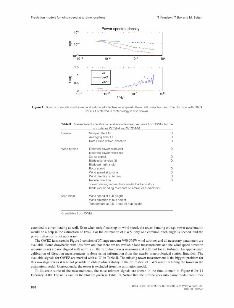
Comparing the NWS with the estimated ones in Figure 2 shows that the filter removes the higher frequencies; moreover,the estimates behave as expected. A portmanteau test (see Section 6.6 of Madsen20) with a correct model will show outputprediction errors that are white noise. The model is not perfect as the tower is left out. This is the main reason for the sig-nificant correlation in the residual tests seen in Figure 3. However, these correlations are significant but acceptably small.Figure 4 shows the low-pass behavior of the system in frequency domain. The tower frequency is again hardly visible in

the estimated wind but can be seen at 0.25 Hz in the nacelle wind in the lower plot.

3. FARM AND MEASUREMENTS

The ideal required measurements are stated in Table II. The meteorology mast can give free flow wind speed and directionthat can be useful, but this is not crucial for this investigation. Tower and blade loadings are necessary if the models are


885


10−3 10−2 10−1 10010−5

100

105

Φ(f

)

Power spectral density

10−3 10−2 10−1 1000

0.5

1

1.5f Φ

(f)

f (Hz)

Vn

VeKF

VmKF

Figure 4. Spectra of nacelle wind speed and estimated effective wind speed. There 3600 samples used. The plot type with fˆ.f/versus f preferred in meteorology is also shown.

Table II. Measurement specification and available measurements from OWEZ for thesix turbines WTG2-4 and WTG14-16.

General Sample rate:1 Hz OAveraging time:1 s ODate / Time stamp: absolute O

Wind turbine Electrical power produced OElectrical power referenceStatus signal OBlade pitch angles (3) OBlade azimuth angleRotor speed OWind speed at turbine OWind direction at turbine ONacelle direction OTower bending moments or similar load indicatorsBlade root bending moments or similar load indicators

Met. mast Wind speed at hub heightWind direction at hub heightTemperature at 0.5, 1 and 1.5 hub height

O, available from OWEZ.

extended to cover loading as well. Even when only focussing on wind speed, the tower bending or, e.g., tower accelerationwould be a help in the estimation of EWS. For the estimation of EWS, only one common pitch angle is needed, and thepower reference is not necessary.

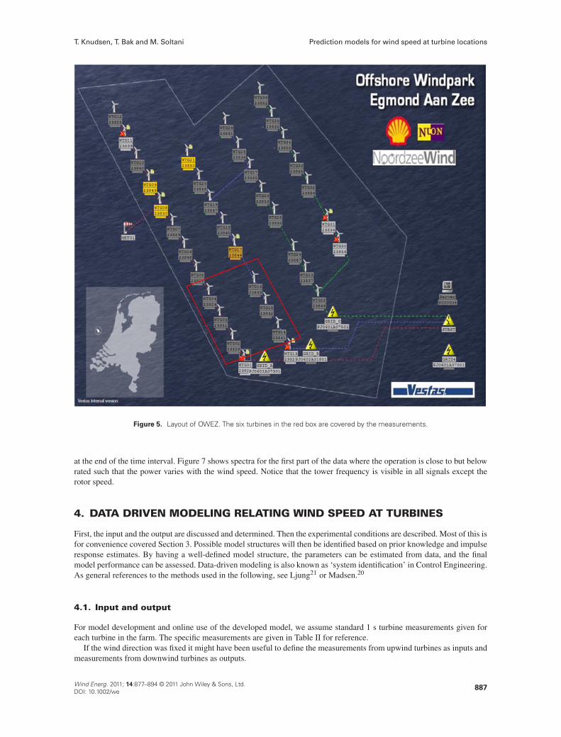
The OWEZ farm seen in Figure 5 consists of 37 large modern V90-3MW wind turbines and all necessary parameters areavailable. Some drawbacks with this farm are that there are no available load measurements and the wind speed directionmeasurements are not aligned with north, i.e., the zero direction is unknown and different for all turbines. An approximatecalibration of direction measurements is done using information from the nearby meteorological station Ijmuiden. Theavailable signals for OWEZ are marked with a ‘O’ in Table II. The missing tower measurement is the biggest problem forthis investigation as it was not possible to obtain observability in the estimation of EWS when including the tower in theestimation model. Consequently, the tower is excluded from the estimation model.

To illustrate some of the measurements, the most relevant signals are shown in the time domain in Figure 6 for 11February 2009. The units used in the plot are given in Table III. Notice that the turbine goes into pause mode three times


DOI: 10.1002/we


Figure 5. Layout of OWEZ. The six turbines in the red box are covered by the measurements.

at the end of the time interval. Figure 7 shows spectra for the first part of the data where the operation is close to but belowrated such that the power varies with the wind speed. Notice that the tower frequency is visible in all signals except therotor speed.

4. DATA DRIVEN MODELING RELATING WIND SPEED AT TURBINES

First, the input and the output are discussed and determined. Then the experimental conditions are described. Most of this isfor convenience covered Section 3. Possible model structures will then be identified based on prior knowledge and impulseresponse estimates. By having a well-defined model structure, the parameters can be estimated from data, and the finalmodel performance can be assessed. Data-driven modeling is also known as ‘system identification’ in Control Engineering.As general references to the methods used in the following, see Ljung21 or Madsen.20

4.1. Input and output

For model development and online use of the developed model, we assume standard 1 s turbine measurements given foreach turbine in the farm. The specific measurements are given in Table II for reference.

If the wind direction was fixed it might have been useful to define the measurements from upwind turbines as inputs andmeasurements from downwind turbines as outputs.


887


x 10

x 10

x 10

x 10

x 10

x 10

05

1015

WTG02WindSpeed

Time (sec.)

250

300

350

WTG02WindDirection

51015

WTG02RotorSpeed

0100020003000

WTG02ProducedPower

0 1 2 3 4 5 6 7 8 9

0 1 2 3 4 5 6 7 8 9

0 1 2 3 4 5 6 7 8 9

0 1 2 3 4 5 6 7 8 9

0 1 2 3 4 5 6 7 8 9

0

20

40WTG02PitchAngle

0 1 2 3 4 5 6 7 8 9260280300320340360380

WTG02NacelleDirection

Figure 6. Time plot for signals from WT02 for 1 day, 11 February 2009.

Table III. Names and units for data in plots. For specific turbines, thenames are pre-pended with WTG fturbine numberg.

Name Unit

OWEZ dataNacelleDirection degreeOperationalState integerPitchAngle degreeProducedPower KWRotorSpeed rpmWindDirection degreeWindSpeed m s�1

Filtered dataWindSpeedE m s�1

In practice, the wind direction varies continuously so no turbine is always upwind and measurements cannot be fixedas inputs or outputs. For a model valid for all wind conditions, this means that all measurements form a very large outputvector, and there are no inputs. In system identification terminology, this is a multidimensional time-series model.

In this paper, a simpler model is used for a start. To this end, data where the wind direction and two turbines areapproximately aligned are selected. Then the measurements on upwind and downwind turbines are input and output,respectively.

Especially for the first 3 h of the data, the average wind direction is close to 320, which is close to the direction of turbinerow 4-3-2 or 16-15-14. Therefore turbine 3 will be used as input and 2 as output. Similar results were obtained using othercombinations of turbines.


DOI: 10.1002/we


10−3 10−2 10−1 100

100

Φ(f

)

Power spectral density

10−3 10−2 10−1 100

0

0.1

0.2

0.3

0.4f Φ

(f)

f (Hz)

WTG02PitchAngle

WTG02ProducedPower

WTG02RotorSpeed

WTG02WindSpeed

Figure 7. Power spectrum for signals from WT02. Time range Œ2 103;2 104�, which is close to but below rated. The plot type withfˆ.f/ versus f preferred in meteorology is also shown.

The wind speed in question here also needs a precise definition. Wind velocity is a vector field from R4 (time and space)to R3 (three-dimensional velocity). As the estimated models are intended for farm control, this means that the faster fre-quencies and smaller spatial scales, e.g., 1 m, are not relevant. The relevant wind speed is the wind speed over the rotor discalso known as the effective wind speed.9,10 Light detection and ranging technique would be an option to measure EWS,but this is not part of ‘standard signals from turbines’, and it is also still expensive. To measure EWS, it is then necessaryto use turbines as measurement devices. This is covered in Section 2. To compare with results in the literature, both pointand effective wind speed will be used in this investigation. Note that it is difficult to directly compare the predictability ofmeasured NWS and EWS as they measure different physical quantities.

4.2. Model structures

The only literature found on these specific models is Nielsen et al.7 Here, an input/output (I/O) model for predicting pointwind speed from measured upwind point wind speed is presented. The model included a stochastic part of ARMA type,which was not important for predictions longer than 20 s. The deterministic part has the form (32) where uj and ui aredownwind and upwind 10 s average point wind speed measured at 80 m height at masts at Høvsøre. Further, U10 is the10 min average wind speed, and d is the distance between locations. This means that the impulse response function h usestime scaling with the time it takes the average wind to move from input to output location.

uj .t/D 0 C

Z 10

h

�U10.t/

ds

�ui .t � s/ds (32)

A similar, but simpler, IO model is a good starting point for the model relating wind speed at upwind and downwindturbines.

4.3. Impulse response estimates

Initially, a nonparametric impulse response is estimated to indicate the type of model needed and to test the delay modelidea coming from the physical interpretation that the turbulence travels downwind as it decays.

The nonparametric impulse response estimate in Figure 8 is for EWS based on the first 8 h. There is a significant ‘hump’centered around 80, which multiplied by average upwind EWS gives 733 m under the given wind conditions that is some-what larger than the inter-turbine distance of 632 m. However, the average upwind EWS corresponds to free/undisturbedwind that is larger than the actual wind in the farm, and this explains most of the mismatch. Nevertheless, this supportsthe existence of a delay. It has been tried to focus on shorter time intervals with varying wind speeds to test if the delayapproximately equals the time it takes the mean wind to travel between turbines. However, reducing to, e.g., 2 h makesalmost all estimates insignificant. Furthermore, the impulse response estimate for NWS was generally insignificant.


889


−100 −50 0 50 100 150 200−0.03

−0.02

−0.01

0

0.01

0.02

0.03

0.04From WTG03WindSpeedE

To

WT

G02

Win

dSpe

edE

Time

Figure 8. Nonparametric impulse response estimate for EWS. Data: 11 February 2009; WT3 to WT2, first 8 h; average wind,9.17 m s�1. The dash-dotted lines are 0.95 significance limits.

4.4. Simple linear time-invariant (LTI) models

In this section, standard LTI models are described. Then the parameters are estimated, and the corresponding 1, 30 and 60 sforecast errors are calculated.

For single-input single-output (SISO) system, an LTI model can be defined as in equation (33). Here, the output y is asum of filtered input u and filtered white noise e. The transfer functionsG andH are defined using the ‘back step operator’q�1 formulation. For more details, see, e.g., Ljung.21

y.t/DG.q�1/u.t � nk/CH.q�1/e.t/; e.t/ 2 ID.0; �2/ (33a)

G.q�1/DB.q�1/

A.q�1/F .q�1/; H.q�1/D

C.q�1/

A.q�1/D.q�1/(33b)

A.q�1/D 1C a1q�1C � � � C anaq

�na D

naXiD0

aiq�i ; a0 D 1 (33c)

B.q�1/D

nbXiD0

biq�i ; C .q�1/D

ncXiD0

ciq�i ; c0 D 1 (33d)

D.q�1/D

ndXiD0

diq�i ; d0 D 1; F .q�1/D

nfXiD0

fiq�i ; f0 D 1 (33e)

This model structure is the most general one among LTI SISO I/O models. To define a specific model structure in this class,the structural parameters na; nb ; nc ; nd ; nf ; nk must be chosen. This investigation should reveal if there is any poten-tial for predicting EWS. Therefore, the following simplifying choices have been made. Autoregressive exogenous (ARX)models where C D D D F D 1 were tested because they give a unique parameter estimate and are fast and robust. Incase of under modeling, standard prediction error methods for ARX structures can give bias for the lower frequencies thatcould give bad performance for long-term prediction. This would then be fixed with an output error (OE) structure whereAD C DD D 1)H D 1 or a Box–Jenkins (BJ) structure where H has separate parameters, i.e., AD 1. As the impulseresponse estimate indicates a delay larger than 50 samples, also models with delay are tested. Test not shown here indicate


DOI: 10.1002/we


optimal delays nk � 60, typically 70; therefore, nk D 60 has been chosen as the input needed for prediction and is thenknown up to prediction horizons of 60 s. A model order of 2 is used for all model structures discussed previously. Thereasons are that second-order models can reproduce the ‘bump’ like impulse response, and there seems to be no substantialimprovement from using higher-order models. To compare with what can be obtained without upwind information, anautoregressive (AR) structure where B D 0 ) G D 0 and C D D D 1 is included as well as the special AR structureA.q�1/D 1� q�1 known as the persistence method where any prediction always equals the last measurement.

For estimation, the first 4 h are used, and for cross validation, the next 4 h are used as illustrated in Figure 9.The most important results are shown in Table IV. The root-mean-square (RMS) error is the standard prediction error

estimate (equation (34)). The fit (35) shows how much of the standard deviation in the output is explained by the model.

0 0.5 1 1.5 2 2.5 3x 104

0

5

10

15

Time

WTG02WindSpeedE

0 0.5 1 1.5 2 2.5

x 104

5

10

15WTG03WindSpeedE

Time

Figure 9. Data to estimate LTI models. First 4 h for estimation, last 4 h for cross-validation. Data: 11 February 2009.

Table IV. Predictability for nacelle wind speed using one upwind turbines and LTI models.

Type OE ARX ARXDel BJDel AR Per

na 0 2 2 0 2 1nb 2 2 2 2 — —nc 0 0 0 2 0 0nd 0 0 0 2 0 0nf 2 0 0 2 — —nk 0 0 60 60 — —

Prediction horizon (s) Fit (%)1 32.149 37.441 37.558 42.233 34.412 28.53530 32.149 21.955 23.943 32.062 �10.935 9.15960 32.149 21.933 23.937 31.548 �63.183 6.0711 32.149 21.933 23.937 32.153

Prediction horizon (s) RMS (m s�1)1 0.886 0.817 0.816 0.755 0.857 0.93430 0.886 1.020 0.994 0.888 1.449 1.18760 0.886 1.020 0.994 0.894 2.132 1.2271 0.886 1.020 0.994 0.886

The columns in the two bottom sections, Fit and RMS, hold the results using the model structure specified in the columnin the top section. The model structures marked with ‘Del’ includes the 60 s delay. Prediction horizon1 corresponds topure simulation. The negative fit values are due to under-modeling, given bias when parameters are optimized for onestep prediction and then used for multistep prediction.


891


RMSD

vuut 1

N

NXtD1

.y.t/� Oy.t jt � k//2 (34)

FitD 1�RMS

O�y(35)

As seen, the maximal fit for 60 s predictions for NWS is less than 1/3 corresponding to a RMS error of 0.9 m s�1, whichis a poor fit. It is obtained with the OE model structure. Even though this is poor, it is far better than that of persistence,which gives a fit of 0.06. The rows marked with 1 are the results from a prediction horizon at infinity meaning that noold outputs are used, only inputs are used to calculate the output, this in turn is also called pure simulation. Notice that theresults are nearly the same as for a prediction horizon at 30 s or more. This means that the stochastic part does not reallyplay a role for variations over 30 s.

For the EWS, the results are shown in Table V. The best results are obtained using 60 s delay and the ARX or BJ model,which for a minute prediction gives an RMS error of 0.33 m s�1 corresponding to a 95% significance limits at˙0:66m s�1,which is small enough to be useful. The results in Nielsen et al.7 for this mean wind speed, which is 8.3 m s�1 for thevalidation data, give a significance interval of ˙0:6 m s�1 but for point wind speed only separated by 300 m. Again, thisis difficult to compare, but at least, there is no clear conflict. Comparing the ARX structure with the persistence methodshows that the prediction error of the former is close to 0.7 of the latter.

The last column in Table V is the results where the ARX structure is used, but the input is now from turbine 4 that isapproximately at double the distance, i.e., 1277 m compared with that of turbine 3, which is 632 m from turbine 2. Thedelay is therefore doubled to nk D 120. It is interesting to see that even at this distance, the 1 min prediction error isreduced to approximately 0.82 compared to persistence. For EWS, the stochastic part is seen to play a slightly bigger role.Still, it does not improve the 1 min prediction much over pure simulation.

To give some visual results, Figure 10 zooms in on one of the large gusts in the validation data. Here, it is clearly seenthat a simple prediction model based on the first or second upwind turbine outperforms the persistence method.

4.5. Alternative model structures

For validation, other combinations of wind direction with aligned turbines were tested, e.g., WTG3-4 in Figure 5. Mostof them gave similar results as the ones shown here for WTG2-3. Also, it was tested if the prediction performance wasimprove from including more turbines, e.g., using WTG3, 13 and 14 to predict WTG2. However, this did not improveperformance. Another immediate idea is to include the wind speed direction relative to the direction between turbines. Asthe direction is definitely not expected to enter linearly in the model, nonlinear model structures as, e.g., nonlinear ARXmodels and Hammerstein models21 have been tested. It was not possible to improve on the linear models. The only onethat looked promising was the Hammerstein model where the upwind EWS enters linearly and the relative wind directionenters via a piecewise affine input nonlinearity. The estimated static input nonlinearity is shown in Figure 11. Here, it isseen that the predicted wind speed downwind decreases when the wind direction is closer to the turbine directions; noticealso that there seems to be a bias in the calibration as the input nonlinearity is not an even function.

Table V. Predictability for effective wind speed using one upwind turbine and LTI models.

Type OE ARX ARXDel BJDel AR Per ARXDel4To2

Prediction horizon (s) Fit (%)1 60.008 94.444 94.466 94.520 94.430 94.380 94.45430 60.008 63.515 68.346 67.928 59.458 59.516 64.84660 60.008 60.958 66.862 66.056 52.253 52.501 61.1781 60.008 62.698 65.208 65.736 55.140

Predicate horizon (s) RMS (m s�1)1 0.397 0.055 0.055 0.054 0.055 0.056 0.05530 0.397 0.362 0.314 0.318 0.403 0.402 0.34960 0.397 0.388 0.329 0.337 0.474 0.472 0.3861 0.397 0.370 0.345 0.340 0.445


DOI: 10.1002/we


Prediction of EWS

6000 6200 6400 6600 6800 70007

7.5

8

8.5

9

9.5

10

10.5

11

Time (sec)

Win

d sp

eed

(m/s

)

MeasuredPerArxDelBJDel−simArxDel4To2

Figure 10. Example of predictions with a gust. Legend: ‘Measured’ simply is the measured EWS on the downwind turbine WT2.The rest of the curves ‘Per’, etc., are 1 min predictions except BJDel-sim that is pure simulation. See the text for further details.

Data: 11 February 2009.

−40 −30 −20 −10 0 10 20 30 40 501.4

1.6

1.8

2

2.2

2.4

2.6Input nonlinearity

Direction (normalized) (deg)

Non

linea

r fu

nctio

n

Figure 11. Hammerstein input nonlinearity for wind direction. Data: 11 February 2009.

5. CONCLUSION

In this paper, an estimator for effective wind speed was developed. This estimator includes the wind speed in a new moreaccurate way compared with the estimators found in the literature. By using the estimator, the effective wind speeds forsix turbines in the OWEZ farm have been estimated. These effective wind speeds are then used for developing modelswith the purpose of predicting wind speed for a turbine up to 1 min ahead using standard measurements from an upwindturbine. Based on simple classical models, the prediction error for this effective wind speed can be reduced by 30% usingan upwind turbine compared with the persistence method. This reduction is for a prediction horizon of 1 mine and a dis-tance of 632 m. The smallest standard deviation for this prediction error is 0.33 m s�1 corresponding to a 95% confidenceinterval at ˙0:66 m s�1, which is sufficiently small to be useful. When the distance is approximately doubled to 1277 m,the reduction falls from 30% to approximately 15%.


893


ACKNOWLEDGEMENTS

This work is supported by the EU project Aeolus under contract number 224548 and by the project CASED founded byDanish Agency for Science Technology and Innovation.

REFERENCES

1. Gjengedal T. Large-scale wind power farms as power plants. Wind Energy 2005: 361–373.2. Bjerge C, Kristoffersen JR. Run an offshore wind farm like a power plant. VGB PowerTech 2007; 87: 63–66. ISBN

1435-3199.3. Maciejowski JM. Predictive Control with Constraints. Prentice Hall, 2002.4. Findeisen R, Imsland L, Allgower F, Foss BA. State and output feedback nonlinear model predictive control: an

overview. European Journal of Control 2003; 9: 190–206.5. Zhao R, Su Y, Knudsen T, Bak T, Shen W. Multi-agent model for fatigue control in large offshore wind farm. In

2008 International Conference on Computational Intelligence and Security (CIS’08); 71–75. IEEE, IEEE ComputerSociety, 2008. ISBN 978-0-7695-3508-1. DOI:10.1109.

6. Sørensen P, Hansen AD, Thomsen K, Buhl T, Morthorst PE, Nielsen LH, Iov F, Blaabjerg F, Nielsen HA, Madsen H,Donovane MH. Operation and control of large wind turbines and wind farms - final report, Technical ReportRisø-R-1532(EN), Risø, 2005.

7. Nielsen HA, Madsen H, Sørensen P. Ultrashort term wind speed forecasting. In European Wind Energy Conference &Exhibition, London, November 2004. EWEA, EWEA, 2004.

8. Panofsky HA, Dutton JA. Atmospheric Turbulence. John Wiley & Sons, 1984.9. Østergaard KZ, Brath P, Stoustrup J. Estimation of effective wind speed. In Journal of Physics: Conference Series 75,

EWEA, IOP Publishing, 2007.10. Leithead WE. Effective wind speed models for simple wind turbine simulations. In BWEA 1992, 1992; 321–326.11. Van der Hooft EL, Van Engelen TG. Estimated wind speed feed forward control for wind turbine operation

optimization. In European Wind Energy Conference, London, ECN, 2004. ECN-RX–04-126.12. Odgaard PF, Damgaard C, Nielsen R. On-line estimation of wind turbine power coefficients using unknown input

observers. In 17th IFAC World Congress, IFAC, IFAC, 2008; 10646–10651.13. Qiao W, Zhou W, Aller JM, Harley RG. Wind speed estimation based sensorless output maximization control for a

wind turbine driving a dfig. IEEE Transactions on Power Electronics 2008; 23(3): 1156–1169.14. Grewal MS, Andrews AP. Kalman Filtering, 2nd edn. Prentice Hall, Inc., 2001.15. Egmond aan zee offshore wind farm. [Online]. Available: http://www.noordzeewind.nl/ (Accessed December 2009).16. Snel H, Schepers JG. Engineering moles for dynamic inflow phenomena. Journal of Wind Engineering and Industrial

Aerodynamics 1992; 39: 267–281. The title says “moles” but the authors meant “models”.17. Burton T, Sharpe D, Jenkins N, Bossanyi E. Wind Energy Handbook. John Wiley, 2008.18. Munteanu I, Bratcu AI, Cutululis N-A, Ceanga E. Optimal Control of Wind Energy Systems. Springer, 2008.19. Papoulis A, Unnikrisha Pillai S. Probability, Random Variables and Stochastic Processes, 4th edn. McGraw-Hill, 2002.20. Madsen H. Time Series Analysis. Chapman & Hall, 2008. ISBN: 978-1-4200-5967-0.21. Ljung L. System Identification, Theory for the User, 2nd edn. Prentice-Hall information and system sciences series.

Prentice-Hall, 1999.


DOI: 10.1002/we

Documents

Aalborg Universitet Prediction models for wind speed at