Aalborg Universitet

Evaluation of Reliability in Risk-Constrained Scheduling of Autonomous Microgridswith Demand Response and Renewable Resources

Vahedipour-Dahraie, Mostafa; Anvari-Moghaddam, Amjad; Guerrero, Josep M.

Published in:IET Renewable Power Generation

DOI (link to publication from Publisher):10.1049/iet-rpg.2017.0720

Publication date:2018

Document VersionAccepted author manuscript, peer reviewed version

Link to publication from Aalborg University

Citation for published version (APA):Vahedipour-Dahraie, M., Anvari-Moghaddam, A., & Guerrero, J. M. (2018). Evaluation of Reliability in Risk-Constrained Scheduling of Autonomous Microgrids with Demand Response and Renewable Resources. IETRenewable Power Generation, 12(6), 657-667. https://doi.org/10.1049/iet-rpg.2017.0720

General rightsCopyright and moral rights for the publications made accessible in the public portal are retained by the authors and/or other copyright ownersand it is a condition of accessing publications that users recognise and abide by the legal requirements associated with these rights.

? Users may download and print one copy of any publication from the public portal for the purpose of private study or research. ? You may not further distribute the material or use it for any profit-making activity or commercial gain ? You may freely distribute the URL identifying the publication in the public portal ?

Take down policyIf you believe that this document breaches copyright please contact us at vbn@aub.aau.dk providing details, and we will remove access tothe work immediately and investigate your claim.

1

Evaluation of Reliability in Risk-Constrained Scheduling of Autonomous Microgrids with Demand Response and Renewable Resources

Mostafa Vahedipour-Dahraie 1*, Amjad Anvari-Moghaddam2, Josep M. Guerrero 2 1 Department of Electrical and Computer Engineering, University of Birjand, Birjand, Iran.

2 Department of Energy and Technology, Aalborg University, Aalborg, Denmark. *vahedipour_m@birjand.ac.ir

Abstract: Uncertain natures of the renewable energy resources and consumers’ participation in demand response (DR) programs have introduced new challenges to the energy and reserve scheduling of microgrids, particularly in the autonomous mode. In this paper, a risk-constrained stochastic framework is presented to maximize the expected profit of a microgrid operator under uncertainties of renewable resources, demand load and electricity price. In the proposed model, the trade-off between maximizing the operator’s expected profit and the risk of getting low profits in undesired scenarios is modeled by using conditional value at risk (CVaR) method. The influence of consumers’ participation in DR programs and their emergency load shedding for different values of lost load (VOLL) are then investigated on the expected profit of operator, CVaR, expected energy not served (EENS) and scheduled reserves of microgrid. Moreover, the impacts of different VOLL and risk aversion parameter are illustrated on the system reliability. Extensive simulation results are also presented to illustrate the impact of risk aversion on system security issues with and without DR. Numerical results demonstrate the advantages of customers’ participation in DR program on the expected profit of the microgrid operator and the reliability indices.

Nomenclature

Indices

(.).,t,s At time t in scenario s.

i,w,v,j Indices of DGs, wind turbines, PV units

and group of customers.

t,s Indices of time slots and scenarios.

b, n, r Indices of system buses.

Parameters and constants

jD

Base load of customer j (kW).

β Risk-aversion parameter. Per unit confidence level.

T Time interval (hour).

twc , , tvc , Cost of wind and PV energy ($).

tjc , Electricity price offered to customers

($/kWh). upRtic , (

dnRtic , )

Bid of up (down)-spinning reserve

submitted by DG i in period t ($/kWh). upRtjc , (

dnRtjc , )

Bid of up (down)-spinning reserve

submitted by load j in period t ($/kWh). nonRtic ,

Bid of non-spinning reserve submitted by

unit i in period t ($/kWh).

ttjE ,, (htjE ,,

)

Self-elasticity (cross-elasticity) of load j.

GN , WN , VN

Number of DG, wind and PV units.

SN , TN , JN Number of scenarios, time slots and

group of customers.

Pimax (Pi

min) Maximum (minimum) generating

capacity of DG i (kW).

Djmax ( Dj

min) Max/min load of customers’ j (kW).

s Probability of scenario s.

rnG , ( rnB , )

Conductance (susceptance) of line that

connected node n to node r.

xM

Set of generating units x (load x) into the

set of nodes.

Set of lines.

Variables LC

stjD ,, Involuntary load curtailment (kW).

LSstjD ,,

Involuntary load shifting (kW).

PstrnLF ,,, ,

(Q

strnLF ,,, )

Active (reactive) power flow from node n

to r (kW).

stiP ,, Scheduled power for DG i (kW).

stwP ,, ( stvP ,, )

Output power of WT w (PV v) (kW).

dnstiR ,, (

dnstjR ,, ) Down-spinning reserve deployed by unit

i (load j). non

stiR ,, Non-spinning reserve deployed by DG i.

shed

stjL ,, Inelastic load shedding level of j-th load

(kW).

stn ,,

Voltage angle at node n (rad).

stnV ,, Voltage magnitude (RMS value) at node

n (pu.).

stiSU ,, Startup cost of DG i ($).

stiSD ,, Shute down cost of DG i.

stiu ,, Commitment status of DG i {0, 1}.

stiy ,, , stiz ,, Startup and shutdown indicators of DG i.

1. Introduction

In recent years, demand-side management (DSM) has

been contemplated as a crucial option in most energy policy

decision-making. In restructured power systems, the scope

of DSM has also been considerably expanded to include

demand response (DR) programs [1]. DR programs provide

many potential benefits such as reduction of operating cost

2

and emission [2], improvement of system reliability [3],

shaping of daily load profile [4]-[5] as well as providing

financial incentives to customers to benefit from lower

hourly demands [6]. In addition, advent of microgrids in

modern power systems has provided a high potential to

facilitate the active participation of end-use consumers in

DR programs [7]. However, increasing penetration level of

renewable energy sources (RESs) and also, active

participation of customers in DR programs increase

uncertainties in the network which in turn cause imbalances

between the production and consumption and deterioration

of the system reliability [8]-[9]. Hence, it is necessary to

efficiently manage operation of such systems in presence of

uncertainties.

Value of lost load (VOLL) as an important measure in

electricity market can be utilized to control the imbalances

between generation and consumption [10]. VOLL can

profoundly affect the voltage and frequency, spinning and

non-spinning reserve (non-SR) allocation, operating costs as

well as active and reactive losses of the system [11]. The

level of operation security under different uncertainties can

also be distinguished by the VOLL [11]. In other word,

optimal selection of VOLL can result in a low-cost

operation with a high level of security under the existing

uncertainties in the network [12].

The uncertainties associated with RESs, electricity

demand and electricity price in the day-ahead market can

introduce risk into energy and reserve scheduling problem.

In such condition, risk measuring plays a fundamental role

in optimization under uncertainty, providing valuable

information to decision makers. In some literature, risk

aversion on expected cost variability is considered using

conditional value-at-risk (CVaR) approach, avoiding over-

conservative solutions [12-19]. For example, in [13] a risk

averse profit-based optimal operation framework of a

combined wind farm-cascade hydro system has been

proposed in an electricity market, using hydro plants to

compensate wind power forecast errors. An optimal

integrated participation model has been proposed in [14], for

profit enhancement of distributed resources and DR in

microgrids considering system uncertainty. Moreover, a

decision-making strategy for optimal pairing of wind and

DR resources has proposed in [15]. The proposed strategy

applied a paired resource, such as DR or storage to mitigate

the generation scheduling errors inherited in stochastic

technologies. In [16], a decision making model has been

proposed for coordinated operation of wind power producers

and DR aggregators participating in the day-ahead market.

A minimum CVaR term has been also included in the model

formulation to account for the uncertainty around the true

outcomes of day-ahead prices and wind energy. Moreover,

in [17], a risk-constrained stochastic programming

framework has been proposed, to maximize the profit of

microgrid aggregators with considering responsive loads.

Authors of [18] has proposed a scenario-based two-stage

stochastic programming model to jointly optimize the

scheduling of several options in a microgrid, including DR,

RESs and energy storage devices. In [19], authors have

proposed a bi-level framework for the problem of decision-

making by an EV aggregator in a competitive environment.

In the same work, CVaR is applied in the decision-making

process to confront the uncertainties in day-ahead and

balancing markets. Moreover, in [20], authors have

presented a risk-constrained two-stage stochastic

programming model from an islanded microgrid operator’s

perspective for energy and reserve scheduling considering

risk management strategy. However, in none of the

reviewed literature, the effects of VOLL indices on

reliability issues of an autonomous microgrid have been

reported.

In this study, a risk-constrained stochastic programming

framework is presented for optimal scheduling of an

autonomous microgrid under uncertainties. Based on this

program, microgrid operator procures energy from local

distributed generation (DG) units and RESs to supply

microgrid customers. The objective is to maximize the

expected profit of the system operator through optimal

scheduling of resources considering risk aversion and

system reliability issues. To deal with various uncertainties,

a risk-constrained two-stage stochastic programming

formulation is proposed. An efficient solution strategy based

on Benders’ decomposition is also developed to solve the

proposed reliability based optimization problem under

uncertainty. As a whole the main contributions of this paper

are as follows:

1) A risk-constrained two-stage stochastic

programming formulation is proposed to represent

the underlying optimization problem where the risk

aversion of the microgrid operator is captured by

using the CVaR approach,

2) A model for joint energy and reserve scheduling is

presented by considering reliability issues as well

as RESs and DR uncertainties that can be easily

adopted by other entities such as a load serving

entity (LSE), a retailer, or a distribution company

(DISCO),

3) An efficient framework is proposed to illustrate the

impacts of different VOLL and risk aversion

parameter on system reliability.

The rest of paper is arranged as follows: In section 2, system

model is explained. In section 3, the proposed risk-neutral

stochastic optimization formulation is described. The

proposed method for solving the scheduling problem is

presented in section 4. Case studies together with simulation

results are presented in section 5. Finally, section 6 draws

the conclusions.

2. System Model Description

In this study, a medium-scale residential autonomous

microgrid is considered with an average hourly load in the

range of hundred kilowatts. It has several DGs such as

micro-turbines, fuel cells and RESs such as wind and PV

units. A simplified graphical description of the proposed

model is shown in Fig. 1. In this model, the microgrid

operator has a take-or-pay contract [21] to buy energy from

various energy sources while it sells electricity to customers

under real-time pricing scheme, which is based on a service

agreement. Customers are also able to respond to electricity

prices by adjusting their loads to reduce consumption costs.

To do so, it is assumed that the customers are equipped with

house energy management controllers (Hex MCs) and

several smart household appliances. Due to geographically

diverse consumers, JN groups of loads are also considered

for evaluating the influence of users’ participation in DR

3

programs. Moreover, the system operator has access to the

required information such as wind speed, solar irradiation,

electricity price, generation unit and network information

for the scheduling horizon. The energy and reserve

scheduling is done in a way to maximize the operator’s

expected profit and to minimize the users’ energy

consumption costs while fulfilling the microgrid security

and technical constraints. Also, reliability of the microgrid

in a risk-constrained scheduling is evaluated with and

without DR participation.

Fore

cast

ing

mo

du

les

Market-based DR programs

Wind speed

Solar irradiation

Electricity price

Group of

customers # 1

... ...Group of

customers # j

Group of

customers # NJ

Microgrid

operator

Energy and reserve scheduling

Dat

ab

ase

Generating units

information

Microgrid

model and data

Customers’

information

1. To obtain maximum profit of operator while fulfilling the technical constraints .

2. To determine hourly energy and reserve capacity allocated by DG units.

3. To specify the amount of MLS in different values of risk aversion and VOLL.

4. To determine accepted load reduction and reserve capacity of responsive loads.

Fig. 1. Schematic representation of the proposed model.

3. Risk-Neutral Stochastic Optimization Formulation

3.1. Incorporating Risk Management

In financial risk management, Value-at-Risk (VaR) is a

widely-used risk measure focusing on the down-side (i.e.,

tail) risk [22]. However, VaR is not a coherent risk measure.

VaR is only coherent when the underlying loss distribution

is normal, otherwise it lacks sub-additively. Also, VaR

measure does not give any information about potential

losses in the (1−α) worst cases, thus calculating VaR

optimal portfolios can be difficult or even impossible [23].

The Conditional Value-at-Risk (CVaR) is closely linked to

VaR, but provides several distinct advantages especially

when the loss distribution is not normal or when the

optimization problem is high-dimensional (as the case we

experienced in this work). Furthermore, in settings where an

investor/system operator wants to form a portfolio of

different assets, the portfolio CVaR can be optimized by a

computationally efficient, linear minimization problem,

which simultaneously gives the VaR at the same confidence

level as a by-product. Bearing all this in mind, the CVaR

measure for a discrete distribution and at a given confidence

level α is defined mathematically as [22, 23]:

).1

1(max

1,

s

N

s

s

S

s

CVaR

(1)

Subject to: 0;0 sss profit (2)

where, α is the confidence level, profits is the profit in

scenario s, s is probability of scenario s and s is an

auxiliary nonnegative variable equals to the difference

between auxiliary variable and the profits when the profits

is smaller than .

Based on (1), if all profit scenarios are equiprobable,

CVaR is computed as the expected profit in the (1 − α) ×

100% worst scenarios. Therefore, CVaR at a given

confidence level α is defined as the expected value of the

profit smaller than (1-α)-quantile of the profit distribution.

In fact, in the proposed scenario-based stochastic

optimization method, α-CVaR represents approximately the

expected profit of the (1-α)×100% scenarios yielding the

lowest profits.

3.2. Objective Function

The objective of microgrid operator is to maximize its

expected profit in an uncertain environment. Therefore, a

risk-constrained two-stage stochastic programming

framework using α-CVaR method is proposed to formulate

the objective function. In this regard, the weighted α-CVaR

value of the profit is added to a risk-neutral optimization

problem through a weighting parameter called risk aversion

factor β. Therefore, the objective is to maximize the

expected profit of the microgrid operator as follows:

CVaRprofitMaxsN

s

ss ..

1

(3)

where the profits in scenario s is defined as:

Jdnup

Gdnnonup

VWG

T S J

N

j

dnstj

Rtj

upstj

Rtj

N

i

dnsti

Rti

nonsti

Rti

upsti

Rti

N

v

stvtv

N

w

stwtw

N

i

stististi

N

t

N

s

N

j

Shedstj

LSstj

LCstjstjtjss

RcRcRcRcRc

PcPcSDSUPC

LDDDcTprofit

1

,,,,,,

1

,,,,,,,,,

1

,,,

1

,,,

1

,,,,,,

1 1 1

,,,,,,,,,

)..()...(

..].)([

).(..

JN

j

shedstj

LSstj

LSstj LVOLLCC

1

,,,,,, )( (4)

The objective function is the sum of the revenues

obtained from selling electricity to the microgrid customers,

minus the operating cost of DG units (including the cost of

purchasing energy from DGs and their start-up/down cost),

the cost of purchasing energy from wind and PV units, the

cost of reserves allocated to DGs and responsive loads as

well as the payments for the LC and LS and also mandatory

load shedding (MLS). Note that the first line of objective

function represents the base load of group j, minus the

involuntary and mandatory load curtailment. Also, the last

line represents the payment to customers for their

participation in the involuntary load shedding or load

curtailment as well as the cost of expected load not served

for the inelastic loads in working scenarios. In this study, it

is assumed that wind and PV units are not owned by the

microgrid operator, so they are paid a cost-based price for

the electricity they supply to the grid.

3.3. Constraints of the Problem

The proposed objective function is subject to the

following constraints:

4

1) Active and reactive power balance: Power supplied from

committed units and renewable resources must satisfy the

load demand.

Equations (5)-(6) describe the constraints of active and

reactive power balance on bus n at time t and scenario s. The

last terms of these equations stand for the active and reactive

power flow from bus n to bus r represented by (7) and (8),

respectively.

Moreover, equations (9)-(12) represent voltage magnitude

limits, line power flow bounds, emergency load curtailment

limits, and limits of reactive power of DGs. min max

, ,n n t s nV V V (9)

max,

2

,,,

2

,,,max, rn

Qstrn

Pstrnrn LFLFLFLF (10)

tj

shed

stj LL ,,,0

(11)

max

,,

min

istii QQQ

(12)

2) Operation Constraints for DG units: The following

constraints should be met for DGs in each scenario [24]:

iN

m

stmimistiisti PuAPC

1

,,,,,,,, ..)( (13)

mistmi

N

m

stmistiisti PPPuPPi

,,,,

1

,,,,,min

,, 0;.

(14)

Constraint (13) captures the generation cost of DG units that

is approximated by piecewise linear functions [24].

Moreover, output power of DG units obtained by (14). In

these equations, m denotes the indices of segments and Ni

represents the number of segments in the cost function of

unit i, and Ai is the cost of running unit i at its minimum

power generation. Moreover, λi,m is the marginal cost

associated with segment m of cost function unit i, Pi,m is the

upper limit of power generation from the m-th segment of

cost function of unit i and Pi,m,t,s is power generation of unit

i from the m-th segment at time t in scenario s.

stiististiisti zCDSDyCUSU ,,,,,,,, .;. (15)

stiistiististi yPyURPP ,,min

,,,1,,, .)1.( (16)

stiistiististi zPzDRPP ,,min

,,,,,1, .)1.( (17)

stii

UTt

th

sti yUTui

,,

1

,, .

(18)

stii

DTt

th

sti zDTui

,,

1

,, .)1(

(19)

1; ,,,,,1,,,,,,, stistististististi zyuuzy (20)

Constraint (15) represents the limit of the start-up and shut-

down costs of DGs in each scenario. Also, constraints (16)-

(20) denote the limits on ramping rates, minimum ON/OFF

duration, and relationship between binary variables [24].

Note that URi and DRi are the ramping-down and ramping-

up rates limit of unit i and UTi and DTi are the minimum up

and down time of unit i.

In other to fully regulate the frequency, the active power

generation of DGs should be adjusted with respect to the

changes of customers’ consumption. These adjustments

should be done in accordance with active power production

ramp rates, power capacity limits and reserve constraints.

The limits of up, down and non-SRs of DGs are represented

by (21)-(23).

stistiiup

sti PuPR ,,,,max

,,0 (21)

stiistidn

sti uPPR ,,min

,,,,0 (22)

)1(0 ,,max

,,,, stistinon

sti uPR (23)

3) Demand-side constraints: These constraints determine

the degree of participation of each group of customers in

energy and reserve scheduling. For each group of customers

the following criteria must be met: max,,,

min, tjstjtj DDD (24)

min,,,,,0 tjstj

upstj DDR (25)

stjtjdn

stj DDR ,,max,,,0 (26)

4) Relationship between scheduled and deployed reserves:

The relationship between the DG units scheduled and

deployed reserves limits are represented by (27)-(29).

up

stiup

sti Rr ,,,,0

(27)

dnsti

dnsti Rr ,,,,0

(28)

nonsti

nonsti Rr ,,,,0

(29)

Similarly, the relationship between the responsive loads

scheduled and deployed reserves limits are represented by

(30)-(31). up

stjup

stj Rr ,,,,0

(30)

dnstj

dnstj Rr ,,,,0

(31)

5) Linking constraints: These constraints relate market

decisions to the real-time operation of the microgrid through

the deployment of reserves provided by DG units and

),(),(:

,,,,,,,,,

),(),(:

,,

),(),(:

,,

),(),(:

,,

),(),(:

,,

)(

strnr

Pstrn

shedstj

LSstj

LCstj

stMnjj

stj

stMnvv

stv

stMnww

stw

stMnii

sti

LFLDDD

PPP

L

VWI

((5)

),(),(:

,,,,,,,,,

),(),(:

,,

),(),(:

,,

),(),(:

,,

),(),(:

,,

)(

strnr

Qstrn

shedstj

LSstj

LCstj

stMnjj

stj

stMnvv

stv

stMnww

stw

stMnii

sti

LFQQQQ

QQQ

L

VWI

(6)

)sin(..

)cos(.

,,,,,,,,,

,,,,,,,,2

,,,,,,

strstnstrstnrn

strstnstrstnstnrnP

strn

VVB

VVVGLF

(7)

)sin(..

)cos(.

,,,,,,,,,

,,,,,,,,2

,,,,,,

strstnstrstnrn

strstnstrstnstnrnQ

strn

VVG

VVVBLF

(8)

5

responsive loads. The constraints (32)-(33) couple the first

stage decisions with possible realizations of stochastic

processes. dn

stinon

stiup

stitisti rrrPP ,,,,,,,,,

(32)

dnstj

upstjtjstj rrDD ,,,,,,,

(33)

3.4. Economic Model of DR

The consumers' loads are generally divided into three

categories: shiftable, sheddable and non-sheddable loads.

Sheddable loads are those that can be curtailed or turned-off

by the consumer or the system operator without causing any

disruption to the lives, security issues or irreparable harms.

Shiftable loads are related to such consumption units that

must be run in the course of a day; however, there is no

specific run time for them. Therefore, customers participate

in DR program using two general categories of electrical

devices including sheddable and shiftable loads by using

load curtailment (LC) and load shifting (LS) options,

respectively [25]. An economic model for the participation

of customers in DR programs can be developed based on

user’s load reduction in terms of LC/LS mechanisms.

However, the amount of load reduction depends on the

demand elasticity of customers and electricity prices.

Demand elasticity is defined as demand sensitivity to the

price signal. It is comprised of self-elasticity and cross-

elasticity coefficients. Self-elasticity represents changes in

demand due to changes in price at the same time instant t

and can be written as [26]:

tj

tj

tj

tjttj

c

D

D

cE

,

,

int,

int,

,, .

(34)

where,int,tjD is the initial value of demand associated with

customers of group j and

int,tjc is the initial value of electricity

price. In this way, LC can be represented by self-elasticity.

By the same token, LS can be represented by cross-elasticity

which denotes the consumer’s multi-period sensitivity with

respect to the price. To achieve maximum benefit, each

group of customers applies both LC and LS options and

changes their consumption from int,tjD to tjD , in period t as:

tjtjtj DDD ,int,,

(35)

The benefit of group j can be calculated as:

tjtjtjtj cDDBDS ,,,, .)()( (36)

where, )( ,tjDS and )( ,tjDB represent benefit and income of

group j at period t after implementing DR program. To

maximize the benefit of group j, the following criteria must

be met:

0)()(

,,

,

,

,

tj

tj

tj

tj

tjc

D

DB

D

DS

(37)

Among commonly-used functions, the quadratic form is the

most pessimistic model and the most usual customers’

utility function [26]. Based on a quadratic model of DR, the

utility of group j of customers is obtained as [26]:

1)(

1

.)(

1,,

int,

,

1,,

,,0,,

ttjE

tj

tj

ttj

tjtjtjtj

D

D

E

DcBDB

(38)

Differentiating (38) with respect to tjD , and substituting

into (37) gives:

1).()).(1(1

,,

int,

,1,,int

,

,

,

int,1

,,

ttjE

tj

tjttj

tj

tj

tj

tjttj

D

DE

D

D

c

cE

(39)

Therefore, the consumption of group j at time t is obtained

as follows:

1]1

1.[

1,,

1,,

int,

,int,,

ttjE

ttjtj

tjtjtj

Ec

cDD (40)

Furthermore, the amount of demand after DR using cross-

elasticity [26], which modeled LS option, can be obtained

as:

T

ttj

N

htt

E

ttjtj

tjtjtj

Ec

cDD

11

,,int,

,int,,

,,]1

1[. (41)

When the customers of group j participate in DR using both

LC and LS options, the total demand can be calculated as:

TN

h ttjtj

tjttjtjtj

Ec

cEDD

11

,,int,

,,,

int,, ]

1

1ln[.exp.

(42)

4. Proposed Solution Methodology

Fig. 2 illustrates the flowchart of the proposed method for

solving the optimal scheduling problem in a microgrid. This

flowchart has three stages. In the first stage, the structure of

demand that is specified by customers’ electrical devices

and equipment is determined. After customers’ registration,

their total loads are categorized as shiftable, sheddable and

non-sheddable loads and are considered as input data for the

next stage. In the second stage scenario generation and

reduction process is done for stochastic parameters. In this

regard, forecasting errors of stochastic variables are

modeled as continuous probability density functions (PDF)

with a zero-mean normal distribution and different standard

deviations. Monte Carlo simulation (MCS) and roulette

wheel mechanism (RWM) are also used to generate a large

number of scenarios representing the uncertain parameters

based on their corresponding PDFs over the examined

period [27]. Each scenario captures the information of the

hourly wind speed, the hourly irradiation and the hourly

load in the operating day. It should be noted that the

selection of an appropriately sized set of scenarios has been

done based on a trade-off between tractability issues and

problem representation issues using the sample average

approach method detailed in [28]. To mitigate the

computational burden of the stochastic procedure, K-means

algorithm [29] is then applied to reduce the number of

scenarios into a smaller set representing well enough the

uncertainties. Finally, the proposed optimization model is

solved by employing a risk-constraints stochastic

programming approach for each scenario. In this stage, the

reduced scenarios are applied to the proposed model to

maximize the expected profit of islanded MG while

considering system security constraints and reliability

issues. As shown, the solution method includes a master

problem and a sub-problem in which Benders

decomposition (BD) theory [30] is applied for problem

6

solving. In the master problem, unit commitment (UC),

economic dispatch and also the amount LC/LS in DR

programs are determined in a MIP-based problem. Sub-

problem solves, instead, a nonlinear programming problem

representing hourly AC security-constrained optimal power

flow. The solution generated by the upper layer (master

problem) is then considered in the sub-problem and the

feasibility and optimality of the optimal decision of base

case decisions is evaluated under system contingencies to

detect flow violations. If sub-problem fails to get a feasible

solution, an infeasibility cut based on the BD theory is

created accordingly and included to the master problem to

recalculate the dispatch and hourly commitment states of the

generating units and also responsive loads condition.

Collect load data obtained from customers’

registration

Obtain mean and standard deviation through

forecasted and historical data

Scenario generation for load, electricity price,

wind and PV power by using MCS and RWM

Scenario reduction to Ns scenarios by using K-

means method

Master problem

(Find the optimal solution for UC and economic

dispatch without network constraints)

Start

t = 0

s = 0

s < NS

t < NT t = t+1

s = s+1

Number of cuts>0Get the optimal

solution

Add cuts to master

problem

Is it feasible?

Yes

Yes

YesNo

No

Yes No

Subproblem for scenario s

(Hourly evaluation of AC constraints for scenario s)

Identify types of loads and their average power

consumption

Identify demand elasticity of end-users based

on historical data

Input historical data of wind

and PV power

Create cut for

scenario s, time t

No

Yes

Sta

ge 1

: D

ete

rmin

ing

dem

and r

espon

se s

tru

ctu

reS

tage 2

: S

cen

ari

o

gener

ati

on

and r

educti

on

Stage 3:

Scheduling

Determine total demand of all customers

(shiftable, sheddable and non-sheddable loads)

Fig. 2. Flowchart of the proposed solution methodology.

5. Simulation and Numerical Results

5.1. Case Study

The low-voltage autonomous microgrid, as shown in Fig.

3, is considered in order to demonstrate the effectiveness of

the proposed approach. The mass flow of data that is

exchanged between the local controllers (LCs), (Hex MCs)

and the energy management controller (EMC) as well as the

power flow direction are shown. Moreover, in the proposed

scheme DR consists of fully automated signaling from a

utility (which is the microgrid operator in our case) to

provide automated connectivity to end-use customers’

control systems and strategies. The microgrid has five

controllable DG units including two micro-turbines (MT1 &

MT2), two fuel cells (FC1 & FC2), and one gas engine (GE)

with the technical information given in [20]. Additionally,

three similar wind turbines, each with a capacity of 80 kW

and two similar PV plants, each with a capacity of 70 kW

are considered in the examined microgrid. The detailed data

regarding the operating range of the units and their energy

and reserve costs are given in Table 1, [20], [31]. The

microgrid feeds eight groups of aggregated loads that are

equipped with proper controllers to participate in DR

programs. The hourly total load, output power of wind and

PV units and also the hourly electricity price in different

scenarios for one day are shown in Fig. 4. The dashed blue

lines in this figure show the mean of each stochastic

parameter that are equivalent to the forecasted values of

related variable which extracted from [20], [31]. The PDF of

each stochastic parameter is calculated based on previous

records of that parameter for the examined environment.

Here, the PDFs are divided into seven discrete intervals with

different probability levels. It should be mention that real-

time pricing tariff adopted in this study is obtained based on

the stability margin index (SMI) concept that is proposed in

[32] by the authors. Also, standard deviation of the wind

power, PV power, electricity price and load demand forecast

errors are ±10%, ±10%, ±15%, and ±20%, respectively [31]-

[33].

MT1

FC1

PV1WT1

WT2

FC2

PV2

MT2

WT3

Main-Grid

20/ 0.4 kV

MGCC

Static

Switch

1

2

3

7

5

6

4

8

9

13

14

10

15

1612

11

EMS

LC

LC

LC

LC

MG Operator

Hex MCs

Load 1

Hex MCs

Load 5

Hex MCs

Load 2

Hex MCs

Load 7

Hex MCs

Load 3

Hex MCs

Load 4

Hex MCs

Load 6Hex MCs

Load 8

GE

LC

Data flow EMS & HexMCs

Data flow EMS & DG Units

Power flow

LC Local controller of DGs House energy

management controllers Hex MCs

Fig. 3. Single line diagram of the studied microgrid.

7

(a) Scenarios of demand load

(b) Scenarios of wind power

(c) Scenarios of PV power

(d) Scenarios of electricity price

Fig. 4. Scenarios(grey lines) and the mean (dashed blue

lines) of each stochastic parameter

A number of 2000 initial scenarios are generated using

MCS and RWM strategies to model the forecasting errors.

Then, K-means algorithm is implemented to reduce the

initial scenarios into a set of 25 selected scenarios that

represent well enough the uncertainties. The real-time

pricing tariff obtained based on the proposed method in

[32], is used to encourage the customers to participate in DR

programs. Also, the total load has been created by

aggregating the demands of 200 residential homes. The type

of sheddable and shiftable loads and their average power

consumption level for one residential home are illustrated in

Tables 2 and 3, respectively [25].

In this study, the scheduling horizon is considered one

day which is divided into 24 equal time slots. Finally, the

reduced scenarios are applied to a risk-constrained two-stage

optimization model to maximize the expected profit of

microgrid operator. The optimization is carried out by

CPLEX solver using GAMS software [34] on a PC with 4

GB of RAM and Intel Core i7 @ 2.60 GHz processor.

Table 2 Type of sheddable loads and their average power

consumption level for one residential home.

(h) Sheddable

loads

Power

(W)

(h) Sheddable

loads

Power

(W)

1

2

3

4

5

6

7

8

9

10

11

12

Group A*

Group A

Group A

Group A

Group A

Group A

Group B**

Group B

Group B

Group B

Group B

Group B

200

200

200

200

200

200

1300

1550

1550

1550

1550

1550

13

14

15

16

17

18

19

20

21

22

23

24

Group B

Group B

Group B

Group B

Group B

Group B

Group B

Group B

Group B

Group B

Group B

Group B

1550

1300

1300

1300

1550

1550

1550

1550

1550

1550

1300

1300

* Group A: Electrical equipment up to 200W

**Group B: Fans, air conditioners, computers, hairdryer,

coolers, extractor hoods, and other electrical equipment up to

1000W

Table 3 Type of shiftable loads and their average power

consumption level for one residential home.

Average

power

(W)

Type of

shiftable

load

Average

power (W)

Type of

shiftable

load

2000 Dishwashers 1200 Vacuum

cleaners

1000 Meat grinders 2500 Washing

machines 1000 Irons 1800 Dryers

0 2 4 6 8 10 12 14 16 18 20 22 24200

300

400

500

600

700

800

Time (hours)

Load

(kW

)

0 2 4 6 8 10 12 14 16 18 20 22 2410

20

30

40

50

60

Time (hours)

Win

d p

ow

er (

kW

)

0 2 4 6 8 10 12 14 16 18 20 22 240

10

20

30

40

Time (hours)

PV

pow

er (

kW

)

0 2 4 6 8 10 12 14 16 18 20 22 240.05

0.10

0.15

0.20

Time (hours)

Ele

ctri

city

pri

ce (

$/k

Wh

)Table 1 Data of range of units’ production and their energy and reserve costs.

-Cost of non

($) SR

-Cost of down

($) SR

Cost of

($) SR-up

Shut-down

cost ($)

Start-up

cost ($)

Marginal cost

($/kWh)

Min-Max generation

capacity (kW) Unit

0.030 0.030 0.031 0.080 0.090 0.055 25-150 1MT

0.030 0.030 0.031 0.080 0.090 0.068 25-150 2MT

0.035 0.035 0.038 0.090 0.160 0.120 20-100 1FC

0.035 0.035 0.038 0.090 0.160 0.142 20-100 2FC

0.035 0.037 0.039 0.080 0.120 0.084 35-150 GE

- - - - - 0.055 0-80 WT

- - - - - 0.065 0-70 PV

8

5.2. Numerical Results

The expected profit of the microgrid operator versus

CVaR for different levels of risk aversion with and without

DR is shown in Fig. 5. Here, the confidence level to

compute CVaR is considered 95% in all instances. To avoid

crowding data, the optimal solution of the maximization

problem is obtained only for 13 values of β by modifying

risk aversion parameter from 0.01 to 2 as shown in the

figure. Risk aversion parameter models the trade-off

between the expected profit and the profit variability

(measured in terms of CVaR). The efficient frontiers are

obtained for two amounts of VOLL =1 $/kWh and 5 $/kWh

to demonstrate the effects of VOLL. As shown, by

increasing β, CVaR increases and the operator’s expected

profit decreases in all cases. At the first point (e.g., β =0.01),

which shows a solution with a near-zero risk aversion, the

maximum profit at the minimum CVaR is attained. By

increasing β, the total expected profit decreases, however

the average expected profit of the worst-case scenarios

increases, thus, the risk exposure is mitigated. Moreover,

comparison of results in different cases in the same figure

shows that with increasing β, when customers participate in

DR program, the rate of decrement in the expected profit is

lower than that of in case without DR. Also, as observed,

when β increases from 0.01 to 0.1, although the profit does

not change so much, CVaR rises substantially. With further

increase of β, the operator’s expected profit will be

significantly reduced, however CVaR will not be changed so

much. In case of without DR and VOLL=1 $/kWh, the

expected profit and CVaR varies from $287.07 and $113.41

for β = 0 to $281.08 and $168.13 for β = 2, respectively. It

shows a reduction of 2.1% in the expected profit and a

48.2% increase in the CVaR. In case with DR and VOLL=1

$/kWh, the expected profit and CVaR varies from $391.97

and $308.84 for β = 0.01 to $374.65 and $337.96 for β = 2,

respectively, that shows a reduction of 4.4% in the expected

profit and a 9.4% increase in the CVaR. When customers

participate in DR, the uncertainty in system environment

increases which in turn necessitate more reserve allocation

in higher values of β. Hence, the operator encounters lower

expected profit by increasing of β. Moreover, by increasing

the reserve allocation, the MLS in undesired scenarios is

reduced and consequently, the increment percentage of

CVaR decreases.

Fig. 6 shows the expected profit and cost of expected

energy not served (EENS) under different VOLL values in

cases with and without DR actions. As shown in this figure,

without DR, the cost of EENS (payment to customers for

their MLS) increases by increasing VOLL values. Although,

with increasing VOLL the EENS reduces severely, the

product of VOLL and expected EENS increases. Moreover,

for higher values of VOLL, additional SR is much more

cost-effective than the MLS imposed on consumers. Also, in

higher VOLL values, the expensive generating units are

committed to reduce the MLS. Therefore, by increasing the

VOLL, the operator’s expected profit reduces in case

without DR, and even it may be negative (profit losses)

when considered higher values for VOLL. Moreover, in

case with DR support as shown in Fig. 6 (b), demand of

peak periods is decreased by LC/LS activities and as the

result the MLS (as well as the cost of EENS) reduces in

peak hours. Comparison of the results in Fig. 6 (a) and (b)

shows that with customers’ participation in DR program the

operator’s expected profit is increased, especially in higher

values of VOLL.

(a)

(b)

(c)

(d)

Fig. 5. Operator’s expected profit versus CVaR

(a) without DR, VOLL=1 $/kWh

(b) without DR, VOLL=5 $/kWh

(c) with DR, VOLL=1 $/kWh

(d) with DR, VOLL=5 $/kWh

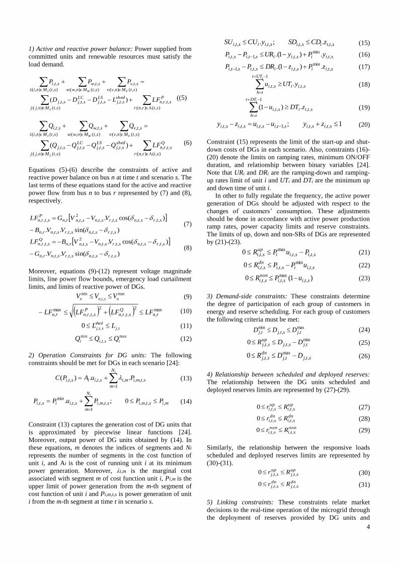
The expected profit versus CVaR for different values of

VOLL at the constant β (i.e., β = 0.01) is shown in Fig. 7. It

is observed that with increasing VOLL both values of

expected profit and CVaR decrease in two cases. Without

DR support, a reduction of 187.4% in the expected profit is

observed, however, in case with DR, this value is 24.1%.

Moreover, with the support of responsive loads in peak

periods and their contributions in better reserve allocation,

the MLS associated with undesired scenarios and

consequently the cost of EENS is decreased substantially.

110 120 130 140 150 160 170280

282

284

286

288

CVaR ($)

Ex

pec

ted

Pro

fit

($)

165 165.5 166 166.5 167 167.5

282.5

283

283.5

284=0.2

=0.4

=0.1

=1.5

=2

=0.6=0.3

=1

=0.01

=0.8

=0.9

=0.7

=0.5

-770 -765 -760 -755 -750 -74554

55

56

57

58

Ex

pet

ed P

rofi

t ($

)CVaR ($)

-751.5 -751 -750.5 -750 -749.5

57

57.5

=0.01

=0.2

=0.4=0.6=0.3

=0.5

=0.1

=0.7=2

=1.5

=1=0.9=0.8

305 310 315 320 325 330 335 340370

375

380

385

390

395

CVaR ($)

Ex

pec

ted

Pro

fit

($)

=0.01

=0.1 =0.3

=2

1.5

=0.4=0.5

=0.6=0.7

=0.8=0.9

=1

=0.2

305 310 315 320 325 330 335 340370

375

380

385

390

395

CVaR ($)

Ex

pec

ted

Pro

fit

($)

=0.01

=0.1

=0.2

=0.3

=0.4

=2

=0.6

=0.7

=0.5

=0.9

=1.5=1=0.8

9

(a)

(b)

Fig. 6. Operator’s expected profit and cost of EENS under

different VOLL values (a) without DR and (b) with DR.

(a)

(b)

Fig. 7. Expected profit versus CVaR for different VOLL

values and β = 0.01

(a) without DR and (b) with DR

Moreover, the expected profit, total cost of scheduled

reserves, cost of MLS with respect to the total load and cost

of ELNS versus VOLL are depicted in Table 4. This table

shows that the reliability of the microgrid and the expected

profit of the operator is largely dependent on the VOLL,

especially in case without DR actions. The microgrid

operator can choose a proper amount of VOLL to keep the

microgrid reliable in order to face the unpredictable

variability of renewable generations and load consumption.

As can be seen from the same table, in case without DR

support, when VOLL increases due to an increment in

EENS, the expected profit decreases, severely. However, in

case of incorporating DR actions, the expected profit has

small variations once VOLL is increasing. As it can be

observed from the table, with DR support, when VOLL is

increased up to 8 $/kWh, no MLS occurs during the entire

scheduling horizon. As a result, in higher values of the

VOLL in which the total scheduled reserve and the ELNS

remain constant, the expected profit remains almost

unchanged. Moreover, with active participation of

customers in DR, a part of up- and down-SR are allocated

by responsive loads and consequently, the amount of these

reserves provided by DGs decrease in case of with DR.

However, the amount of non-SR is increased by DR

participate, since, when the DR is considered, the microgrid

uncertainties are increased and more non-SR is required,

while responsive loads does not able to provide this type of

reserve. Table 5 provides the total amount of spinning (SR)

and non-spinning reserves (non-SR) allocated by DG and

DR resources for different values of VOLL in the 24 hours’

time scheduling. There is no doubt that the equilibrium point

between energy, reserve and EENS can be changed by

increasing the VOLL values. In other word, with increasing

the VOLL, additional SR would be more economic than the

MLS. Thus, as can be observe from the table, the amount of

up- and down-SR increase in higher value of VOLL. The

lowest value of scheduled reserves is attained for VOLL = 1

$/kWh.

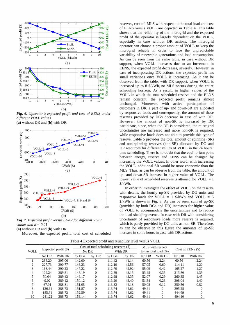
In order to investigate the effect of VOLL on the reserve

with details, the hourly up-SR provided by DG units and

responsive loads for VOLL = 1 $/kWh and VOLL = 5

$/kWh is shown in Fig. 8. As can be seen, sum of up-SR

(provided by both DGs and DR) increases for higher value

of VOLL to accommodate the uncertainties and to reduce

the load shedding events. In case with DR with considering

uncertainty of responsive loads more reserve is required,

which is partly provided by DG units as non-SR. Therefore,

as can be observe in this figure the amounts of up-SR

increase in some hours in case with DR actions.

-300

-200

-100

0

100

200

300E

xp

ecte

d p

rofi

t ($

)

VOLL ($/kWh)

1 2 3 4 5 6 7 8 9 100

100

200

300

400

500

600

Co

st o

f E

EN

S (

$)

Profit

EENS

388.5

389

389.5

390

390.5

391

391.5

392

Ex

pecte

d p

rofi

t ($

)

VOLL ($/kWh)

1 2 3 4 5 6 7 8 9 10296

298

300

302

304

306

308

310

Co

st o

f E

EN

S (

$)Profit

EENS

-2000 -1600 -1200 -800 -400 0 400-400

-200

0

200

400

CVaR ($)

Ex

pec

ted

pro

fit

($)

VOLL=6

VOLL=8

VOLL=9

VOLL=7

VOLL=5

VOLL=3

VOLL=2

VOLL=4

VOLL=1

VOLL=10

296 298 300 302 304 306 308 310388

389

390

391

392

393

CVaR ($)

Ex

pec

ted

pro

fit

($)

VOLL=2

VOLL=3VOLL=4

VOLL=6

VOLL=1

VOLL=5

VOLL=7, 8, 9 and 10

Table 4 Expected profit and reliability level versus VOLL

VOLL Expected profit ($)

Cost of total scheduling reserves ($) MLS with respect

to the total load (%) Cost of EENS ($)

No DR With DR

No DR With DR by DGs by DR by DGs by DR No DR With DR No DR With DR

1 288.20 395.06 142.00 0 111.42 41.14 60.56 2.24 60.56 2.24

2 227.73 390.77 146.23 0 112.10 42.56 57.05 0.60 114.11 1.20

3 168.44 390.23 147.22 0 112.70 42.92 55.09 0.42 165.27 1.27

4 109.24 389.81 148.19 0 112.89 43.15 53.45 0.35 213.80 1.39

5 50.04 389.43 149.17 0 112.98 43.35 52.07 0.29 260.35 1.45

6 -9.02 389.12 150.12 0 113.20 43.40 51.34 0.23 308.04 1.40

7 -67.91 388.81 151.05 0 113.32 44.18 50.08 0.12 350.56 0.82

8 -126.61 388.73 151.87 0 113.74 44.62 49.41 0 395.28 0

9 -185.31 388.73 152.59 0 113.74 44.62 49.41 0 444.69 0

10 -241.22 388.73 153.14 0 113.74 44.62 49.41 0 494.10 0

10

Table 5 Impact of VOLL on the total scheduled reserve.

Case VOLL

($/kWh)

Up-

SR

of

DGs

Down-

SR

of

DGs

Non-

SR

of

DGs

Up-

SR

of

DR

Down-

SR

of

DR

Without

DR

1 738 2401 1174 0 0

5 801 2411 1309 0 0

10 844 2419 1358 0 0

With

DR

1 589 1404 1422 149 1136

5 626 1404 1439 210 1140

10 631 1404 1456 250 1144

(a)

(b)

Fig. 8. Hourly up-SR of DG units and responsive loads in

β = 0.01

(a) without DR and (b) with DR.

Table 6 depicts more numerically details about the

expected profit of the microgrid operator, total cost of

scheduled reserves, cost of EENS and the MLS with respect

to the total load in different values of the risk aversion

parameter β. As can be seen, when risk aversion increases,

the total cost of scheduled reserves is increased in both

cases. Moreover, the operator should allocate more reserve

from the resources to have less forced load shedding

encountering with undesired scenarios. Also, by increasing

β, the percentage of MLS over the entire scheduling horizon

is decreased due to more reserves allocated by resources. As

a result, when risk aversion increases, although the expected

profit of operator decreases, the microgrid will be more

reliable under uncertainties.

To evaluate the effect of risk aversion parameter β on the

scheduled reserve, the total amount of different types of

reserve is illustrated in Table 7 for three values of β in

VOLL=1 $/kWh. As can be seen, in the higher value of β,

the amount of total scheduled reserve increases to reduce the

load shedding in undesired scenarios. Hence, without DR

support when risk aversion increase from 0.01 to 2, up-,

down- and non-SR increase 11.8%, 0.56%, and 24%,

respectively. However, when responsive loads participate in

up/down SR, providing of these types of reserves from DGs

decrease, especially in down-SR. To deploy down-SR

customers should be committed and increase their

consumption. Hence, they are more desired to participate in

this type of reserve and therefore, the down-SR of DGs

reduces in case with DR, significantly.

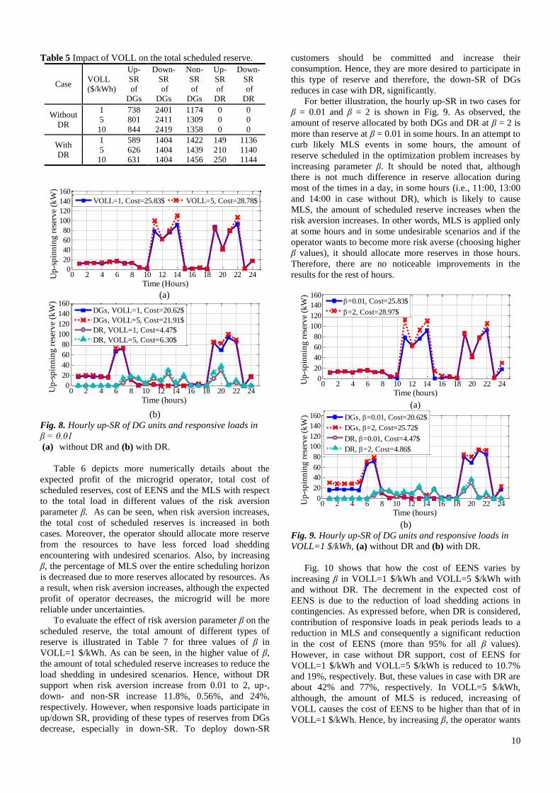
For better illustration, the hourly up-SR in two cases for

β = 0.01 and β = 2 is shown in Fig. 9. As observed, the

amount of reserve allocated by both DGs and DR at β = 2 is

more than reserve at β = 0.01 in some hours. In an attempt to

curb likely MLS events in some hours, the amount of

reserve scheduled in the optimization problem increases by

increasing parameter β. It should be noted that, although

there is not much difference in reserve allocation during

most of the times in a day, in some hours (i.e., 11:00, 13:00

and 14:00 in case without DR), which is likely to cause

MLS, the amount of scheduled reserve increases when the

risk aversion increases. In other words, MLS is applied only

at some hours and in some undesirable scenarios and if the

operator wants to become more risk averse (choosing higher

β values), it should allocate more reserves in those hours.

Therefore, there are no noticeable improvements in the

results for the rest of hours.

(a)

(b)

Fig. 9. Hourly up-SR of DG units and responsive loads in

VOLL=1 $/kWh, (a) without DR and (b) with DR.

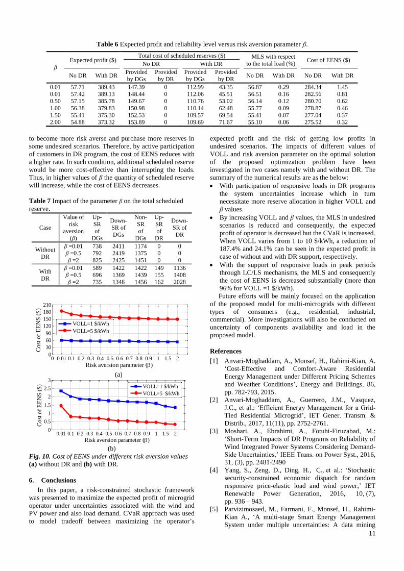
Fig. 10 shows that how the cost of EENS varies by

increasing β in VOLL=1 $/kWh and VOLL=5 $/kWh with

and without DR. The decrement in the expected cost of

EENS is due to the reduction of load shedding actions in

contingencies. As expressed before, when DR is considered,

contribution of responsive loads in peak periods leads to a

reduction in MLS and consequently a significant reduction

in the cost of EENS (more than 95% for all β values).

However, in case without DR support, cost of EENS for

VOLL=1 $/kWh and VOLL=5 $/kWh is reduced to 10.7%

and 19%, respectively. But, these values in case with DR are

about 42% and 77%, respectively. In VOLL=5 $/kWh,

although, the amount of MLS is reduced, increasing of

VOLL causes the cost of EENS to be higher than that of in

VOLL=1 $/kWh. Hence, by increasing β, the operator wants

0 2 4 6 8 10 12 14 16 18 20 22 240

20

40

60

80

100

120

140

160

Time (Hours)

Up

-sp

inn

ing

res

erv

e (k

W)

VOLL=1, Cost=25.83$ VOLL=5, Cost=28.78$

0 2 4 6 8 10 12 14 16 18 20 22 240

20

40

60

80

100

120

140

160

Time (hours)

Up

-sp

inn

ing

res

erv

e (k

W)

DGs, VOLL=1, Cost=20.62$

DGs, VOLL=5, Cost=21.91$

DR, VOLL=1, Cost=4.47$

DR, VOLL=5, Cost=6.30$

0 2 4 6 8 10 12 14 16 18 20 22 240

20

40

60

80

100

120

140

160

Time (hours)

Up

-sp

inn

ing

res

erv

e (k

W)

=0.01, Cost=25.83$

=2, Cost=28.97$

0 2 4 6 8 10 12 14 16 18 20 22 240

20

40

60

80

100

120

140

160

Time (hours)

Up

-sp

inn

ing

res

erv

e (k

W)

DGs, =0.01, Cost=20.62$

DGs, =2, Cost=25.72$

DR, =0.01, Cost=4.47$

DR, =2, Cost=4.86$

11

to become more risk averse and purchase more reserves in

some undesired scenarios. Therefore, by active participation

of customers in DR program, the cost of EENS reduces with

a higher rate. In such condition, additional scheduled reserve

would be more cost-effective than interrupting the loads.

Thus, in higher values of β the quantity of scheduled reserve

will increase, while the cost of EENS decreases.

Table 7 Impact of the parameter β on the total scheduled

reserve.

Case

Value of

risk

aversion

(β)

Up-

SR

of

DGs

Down-

SR of

DGs

Non-

SR

of

DGs

Up-

SR

of

DR

Down-

SR of

DR

Without

DR

β =0.01 738 2411 1174 0 0

β =0.5 792 2419 1375 0 0

β =2 825 2425 1451 0 0

With

DR

β =0.01 589 1422 1422 149 1136

β =0.5 696 1369 1439 155 1408

β =2 735 1348 1456 162 2028

(a)

(b)

Fig. 10. Cost of EENS under different risk aversion values

(a) without DR and (b) with DR.

6. Conclusions

In this paper, a risk-constrained stochastic framework

was presented to maximize the expected profit of microgrid

operator under uncertainties associated with the wind and

PV power and also load demand. CVaR approach was used

to model tradeoff between maximizing the operator’s

expected profit and the risk of getting low profits in

undesired scenarios. The impacts of different values of

VOLL and risk aversion parameter on the optimal solution

of the proposed optimization problem have been

investigated in two cases namely with and without DR. The

summary of the numerical results are as the below:

With participation of responsive loads in DR programs

the system uncertainties increase which in turn

necessitate more reserve allocation in higher VOLL and

β values.

By increasing VOLL and β values, the MLS in undesired

scenarios is reduced and consequently, the expected

profit of operator is decreased but the CVaR is increased.

When VOLL varies from 1 to 10 $/kWh, a reduction of

187.4% and 24.1% can be seen in the expected profit in

case of without and with DR support, respectively.

With the support of responsive loads in peak periods

through LC/LS mechanisms, the MLS and consequently

the cost of EENS is decreased substantially (more than

96% for VOLL =1 $/kWh).

Future efforts will be mainly focused on the application

of the proposed model for multi-microgrids with different

types of consumers (e.g., residential, industrial,

commercial). More investigations will also be conducted on

uncertainty of components availability and load in the

proposed model.

References

[1] Anvari-Moghaddam, A., Monsef, H., Rahimi-Kian, A.

‘Cost-Effective and Comfort-Aware Residential

Energy Management under Different Pricing Schemes

and Weather Conditions’, Energy and Buildings, 86,

pp. 782-793, 2015.

[2] Anvari-Moghaddam, A., Guerrero, J.M., Vasquez,

J.C., et al.: ‘Efficient Energy Management for a Grid-

Tied Residential Microgrid’, IET Gener. Transm. &

Distrib., 2017, 11(11), pp. 2752-2761.

[3] Moshari, A., Ebrahimi, A., Fotuhi-Firuzabad, M.:

‘Short-Term Impacts of DR Programs on Reliability of

Wind Integrated Power Systems Considering Demand-

Side Uncertainties,’ IEEE Trans. on Power Syst., 2016,

31, (3), pp. 2481-2490

[4] Yang, S., Zeng, D., Ding, H., C., et al.: ‘Stochastic

security-constrained economic dispatch for random

responsive price-elastic load and wind power,’ IET

Renewable Power Generation, 2016, 10, (7),

pp. 936 – 943.

[5] Parvizimosaed, M., Farmani, F., Monsef, H., Rahimi-

Kian A., ‘A multi-stage Smart Energy Management

System under multiple uncertainties: A data mining

0 0.01 0.1 0.2 0.3 0.4 0.5 0.6 0.7 0.8 0.9 1 1.5 20

30

60

90

120

150

180

210

Risk aversion parameter ()

Co

st o

f E

EN

S (

$)

VOLL=1 $/kWh

VOLL=5 $/kWh

0.01 0.1 0.2 0.3 0.4 0.5 0.6 0.7 0.8 0.9 1 1.5 20

0.5

1

1.5

2

2.5

3

Risk aversion parameter ()

Co

st o

f E

EN

S (

$)

VOLL=1 $/kWh

VOLL=5 $/kWh

Table 6 Expected profit and reliability level versus risk aversion parameter β.

β

Expected profit ($) Total cost of scheduled reserves ($) MLS with respect

to the total load (%) Cost of EENS ($)

No DR With DR

No DR With DR Provided

by DGs

Provided

by DR

Provided

by DGs

Provided

by DR No DR With DR No DR With DR

0.01 57.71 389.43 147.39 0 112.99 43.35 56.87 0.29 284.34 1.45

0.01 57.42 389.13 148.44 0 112.06 45.51 56.51 0.16 282.56 0.81

0.50 57.15 385.78 149.67 0 110.76 53.02 56.14 0.12 280.70 0.62

1.00 56.38 379.83 150.98 0 110.14 62.48 55.77 0.09 278.87 0.46

1.50 55.41 375.30 152.53 0 109.57 69.54 55.41 0.07 277.04 0.37

2.00 54.88 373.32 153.89 0 109.69 71.67 55.10 0.06 275.52 0.32

12

approach’, Renewable Energy, 102-A, pp. 178-189,

2017.

[6] Aghaei, J., Alizadeh, M.I., Abdollahi, A., Barani, M.:

‘Allocation of demand response resources: toward an

effective contribution to power system voltage

stability’, IET Gener. Transm. Distrib., 2016, 10(16),

pp. 4169-4177

[7] M. Vahedipour-Dahraie, H. R. Najafi, A. Anvari-

Moghaddam, et al.: ‘ Study the Effect of Time-Based

Rate Demand Response Programs on Stochastic Day-

Ahead Energy and Reserve Scheduling in Islanded

Residential Microgrids’, Appl. Sci. 2017, 7 (4), 378,

pp. 1-19

[8] Gholami, A., Shekari, T., Aminifar, F., Shahidehpour,

M.: ‘Microgrid Scheduling with Uncertainty: The

Quest for Resilience’, IEEE Trans smart grid 2016,

30(3), pp. 1337-1350

[9] Moshari, A., Ebrahimi, A., Fotuhi-Firuzabad, M.:

‘Short-Term Impacts of DR Programs on Reliability of

Wind Integrated Power Systems Considering Demand-

Side Uncertainties’, IEEE Trans on Power Syst. 2016,

31(3), pp. 2481-2490

[10] Aghaei. J., Alizadeh, M.I., Siano, P., Heidari, A.,

‘Contribution of emergency demand response

programs in power system reliability’, Energy, 2016,

103, pp. 688-696

[11] Aghaei, J., Nikoobakht, A., Sian, P., Nayeripour, M.,

Heidari, A., Mardaneh, M., ‘Exploring the reliability

effects on the short term AC securityconstrained unit

commitment: A stochastic evaluation’, Energy, 2016,

114, pp. 1016-1032

[12] Wang, J., Shahidehpour, M., Li, Z., ‘Security-

constrained unit commitment with volatile wind power

generation’, Power Syst IEEE Trans. 2008, 23, pp.

1319-27

[13] Moghaddam, I.G., Nick, M., Fallahi, F., et al.: ‘Risk-

averse profit-based optimal operation strategy of a

combined wind farm-cascade hydro system in an

electricity market’, Renew. Energy, 2013, 55, pp. 252–

259

[14] Shayeghi, H., Sobhani, B.: ‘Integrated offering strategy

for profit enhancement of distributed resources and

demand response in microgrids considering system

uncertainty,’ Energy Conv. Manage., 2014, 87, pp.

765–777

[15] Anderson, C.L., Cardell, J.B.: ‘A decision framework

for optimal pairing of wind and demand response

resources’, IEEE Systems Journal, 2012, 29, (1), pp.

149–159

[16] Garcia-Bertrand, R.: ‘Sale prices setting tool for

retailers’, IEEE Trans. Smart Grid, 2013, 4, (4), pp.

2028–2035

[17] Carrion, M., Philpott, A.B., Conejo, A.J., et al.: ‘A

stochastic programming approach to electric energy

procurement for large consumers’, IEEE Trans. Power

Syst., 2007, 22, (2), pp. 744–754

[18] Wang, H., and Jianwei H.: ‘Joint investment and

operation of microgrid’, IEEE Trans. Smart Grid,

2017, 8 (2), pp. 833-845

[19] Rashidizaheh-Kermani, H., Vahedipour-Dahraie, M.,

Najafi, H.R., et al.: ‘A Stochastic Bi-Level Scheduling

Approach for the Participation of EV Aggregators in

Competitive Electricity Markets’, Appl. Sci. 2017, 7,

pp. 1-16

[20] Vahedipour-Dahraie, M., Rashidizaheh-Kermani, H.,

Najafi, H.R., et al.: ‘Stochastic Security and Risk-

Constrained Scheduling for an Autonomous Microgrid

with Demand Response and Renewable Energy

Resources’, IET Renewable Power Generation, 2017,

11(14), pp. 1812-1821.

[21] Conti, S., Nicolosi, R., Rizzo, S.A., Zeineldin, H.H.:

‘Optimal dispatching of distributed generators and

storage systems for MV islanded microgrids’, IEEE

Trans. Power Deliv., 2012, 27, (3), pp. 1243–1251

[22] Choudhry, M.: ‘An Introduction to Value-at-Risk’,

John Wiley & Sons, Third edition, 2006.

[23] Rockafellar, R.T., Uryasev, S., ‘Conditional value-at-

risk for general loss distributions’, Journal of Banking

& Finance, 2002, 26 (7), pp. 1443–1471

[24] Nguyen, DT., Le, LB., ‘Risk-Constrained Profit

Maximization for Microgrid Aggregators with Demand

Response’, IEEE Transactions on smart grid, 2015, 6,

(1), pp. 135-146

[25] Zh, D., Nilay, S., Lazaros, P.: ‘Efficient energy

consumption and operation management in a smart

building with microgrid’, Energy Convers Manag.,

2013, 74, pp. 209-222

[26] Mollahassani-pour, M., Abdollahi, A., Rashidinejad

M.: ‘Investigation of Market-Based Demand Response

Impacts on Security-Constrained Preventive

Maintenance Scheduling’, IEEE Systems Journals

2015, 9(4), pp. 1496-1506

[27] Damousis, I.G., Bakirtzis, A.G., Dokopolous, P.S.: ‘A

solution to the unit-commitment problem using integer

coded genetic algorithm’, IEEE Trans. Power Syst.,

2004, 19(2), pp. 1165-1172.

[28] Eyvindson K., and Kangas A., ‘Evaluating the required

scenario set size for stochastic programming in forest

management planning: incorporating inventory and

growth model uncertainty’, Can. J. For. Res., 46, pp.

340–347, 2016.

[29] Arthur, D., Vassilvitskii, S.: ‘K-means++: The

advantages of careful seeding’, in Proc. 18th Annu.

ACM-SIAM Symp Discrete Algorithms (SODA ‘07),

New Orleans, LA, USA, 2007, pp. 1027-1035

[30] Wang, J., Shahidehpour, M., Li, Z., ‘Security-

constrained unit commitment with volatile wind power

generation’, IEEE Trans. Power Syst., 2008, 23, pp.

1319-1327

[31] Rezaei, N., Kalantar, M.: ‘Stochastic frequency-

security constrained energy and reserve management

of an inverter interfaced islanded microgrid

considering demand response programs’, Int. J. Electr.

Power Energy Syst., 2015, 69, pp. 273–286

[32] Vahedipour-Dahraie, M., Rashidizaheh-Kermani, H.,

Najafi, H.R., et al.: ‘Coordination of EVs Participation

for Load Frequency Control in Isolated Microgrids’,

Appl. Sci. 2017, 7(6), 539, pp. 1-16.

[33] Rezaei, N. Kalantar, M.: ‘Smart microgrid hierarchical

frequency control ancillary service provision based on

virtual inertia concept: An integrated demand response

and droop controlled distributed generation

framework’, Energy Conversion and Management

2015, 92, pp. 287-301

[34] ‘The General Algebraic Modeling System (GAMS)

13

Software’, online available at: http://www.gams.com,

accessed on 15 September 2016