A Zero Phase Shift Band Pass Filter

Hens Steehouwer2,1 Kai Ming Lee2

October 21, 2011

1A�liated with the Econometric Institute, Erasmus University Rotterdam2Ortec Finance Research Center, email: Kai.MingLee@ortec-�nance.com

Introduction

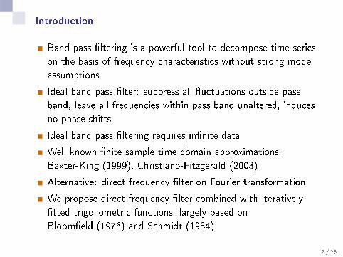
Band pass �ltering is a powerful tool to decompose time series

on the basis of frequency characteristics without strong model

assumptions

Ideal band pass �lter: suppress all �uctuations outside pass

band, leave all frequencies within pass band unaltered, induces

no phase shifts

Ideal band pass �ltering requires in�nite data

Well known �nite sample time domain approximations:

Baxter-King (1999), Christiano-Fitzgerald (2003)

Alternative: direct frequency �lter on Fourier transformation

We propose direct frequency �lter combined with iteratively

�tted trigonometric functions, largely based on

Bloom�eld (1976) and Schmidt (1984)

2 / 28

Ideal band pass �lter

Linear �lter:

G (L) =

b∑k=a

gkLk

applied to series xt gives �ltered series yt = G (L)xt

From the frequency response function (FRF)

G (e−iω) =

b∑k=a

gke−iωk

we obtain

Gain(ω) = |G (e−iω)|

and

Phase(ω) = arg(G (e−iω))/(2π)

3 / 28

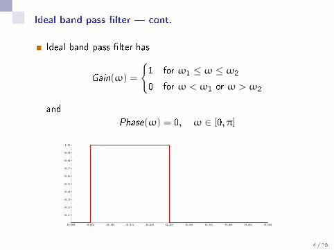
Ideal band pass �lter � cont.

Ideal band pass �lter has

Gain(ω) =

{1 for ω1 ≤ ω ≤ ω2

0 for ω < ω1 or ω > ω2

and

Phase(ω) = 0, ω ∈ [0, π]

0.00 0.05 0.10 0.15 0.20 0.25 0.30 0.35 0.40 0.45 0.50

0.1

0.2

0.3

0.4

0.5

0.6

0.7

0.8

0.9

1.0

4 / 28

Ideal band pass �lter � cont.

Ideal �lter weights in time domain are

gk =

{sin(ω2k)−sin(ω1k)

πk for k 6= 0ω2−ω1π for k = 0

Weights are still substantial at long lags

-100 -80 -60 -40 -20 0 20 40 60 80 100

-0.05

0.00

0.05

0.10

0.15

0.20

5 / 28

Baxter-King and Christiano-Fitzgerald �lter

Baxter-King: truncate weights beyond lag a, impose constraintat frequency ω = 0 (detrending)

Symmetric (no phase shift)

Removes �rst and second order trends

No output for �rst and last a observations

Christiano-Fitzgerald: extrapolate data sample using assumedmodel, adjust end point weights �gk (dependent on assumedmodel for xt)

Filter (and therefore also Gain) is time varying; end point

adjustments for yt depend on t

Weights are asymmetric, so �lter is not phase-neutral

Requires model assumption for xt (recommended: Random

Walk)

6 / 28

Baxter-King Squared Gain

BK(5)

0.00 0.05 0.10 0.15 0.20 0.25 0.30 0.35 0.40 0.45 0.50

0.5

1.0

1.5 BK(5)

BK(20)

0.00 0.05 0.10 0.15 0.20 0.25 0.30 0.35 0.40 0.45 0.50

0.5

1.0BK(20)

BK(100)

0.00 0.05 0.10 0.15 0.20 0.25 0.30 0.35 0.40 0.45 0.50

0.5

1.0BK(100)

(cycles per period)

7 / 28

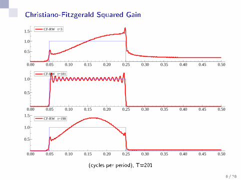
Christiano-Fitzgerald Squared Gain

CF-RW t=3

0.00 0.05 0.10 0.15 0.20 0.25 0.30 0.35 0.40 0.45 0.50

0.5

1.0

1.5 CF-RW t=3

CF-RW t=101

0.00 0.05 0.10 0.15 0.20 0.25 0.30 0.35 0.40 0.45 0.50

0.5

1.0CF-RW t=101

CF-RW t=198

0.00 0.05 0.10 0.15 0.20 0.25 0.30 0.35 0.40 0.45 0.50

0.5

1.0

1.5CF-RW t=198

(cycles per period), T=201

8 / 28

Direct Frequency Filter

1 Calculate the discrete Fourier transform (DFT)

Jj =1

T

T−1∑t=0

xte−iωj t , ωj = 2πj/T ,

for j = 0, . . . ,T − 1.

2 Multiply the Fourier coe�cients Jj with the desired frequency

response function to obtain �Jj .

3 Apply the inverse discrete Fourier transform (IDFT)

xj =

T−1∑j=0

�Jj exp(iωj t)

on �Jt to transform the series back into the time domain.

9 / 28

Direct Frequency Filter � cont.

DFT on �nite data has errors due to leakage

Errors are worse for smaller samples, and for data with higher

peaks in spectrum/periodogram

Upper bound for �lter error due to leakage:

|yt − yt |2 ≤ M2

(∑k∈Q

|gk |)2,

Q = {−∞, . . . , t − T } ∪ {t + 1, . . . ,∞},

where yt is ideal �ltered series, yt is �nite sample direct

frequency �ltered series,

M = max0≤ω≤2π

|T · J(ω)|

J(ω) is continuous extension of Fourier transform

10 / 28

Zero Phase Filter

Direct frequency �lter error can be reduced by increasing

sample (usually impossible), or reducing maximum

periodogram (possible)

Decompose series in �tted trigonometric series and remainder

xt = α cos(θt) + β sin(θt) + rt

Trigonometric component can be �ltered perfectly (avoiding

leakage), and remainder with smaller error than directly

�ltering xt

Use least squares to minimise:

V (α,β, θ) =

T−1∑t=0

(xt − α cos(θt) − β sin(θt)

)211 / 28

Zero Phase Filter � cont.

Sum of squared errors is proportional to Fourier transform,

which gives upper bound to (leakage induced) �lter error.

Optimisation is linear for given θ, non-linear in general

Objective function has many local optimums, so we use

combination of grid evaluation of θ ∈ [0, π] and Brent's

method

Extensions:

Include constant term µ

Fit multiple trigonometric series simultaneously

Fit new trigonometric series on rt , iterate until �nal remainder

is very small

Final �ltered series is sum of �tted trigonometric series with

frequencies θj within the pass band plus direct frequency

�ltered �nal remainder

12 / 28

Zero Phase Filter � cont.

Choices of number of simultaneous components to �t and

stopping criteria for iterations based on simulation and

extensive experience

Majority of the �ltering takes place in time domain, based on

trigonometric �t, and is �ltered with exact pass band

Leakage error in remainder can be made very small by

increasing iterations

Filter induces no phase shift and has no irregularities near end

points

Disadvantage: calculation time is much higher than time

domain approximations or direct frequency �ltering, so e�cient

implementation required

13 / 28

Illustration: Industrial Production Index Finland

IPI_FIN Trend

1960 1965 1970 1975 1980 1985 1990 1995 2000 2005 2010

3.0

3.5

4.0

4.5

5.0IPI_FIN Trend

Bus Mnth

1960 1965 1970 1975 1980 1985 1990 1995 2000 2005 2010

-0.2

-0.1

0.0

0.1Bus Mnth

Trend: (> 8 year), Bus (2�8 year), Mnth (< 2 year)

14 / 28

Illustration: Industrial Production Index Finland

ZP BK(24) CF-RW

1960 1965 1970 1975 1980 1985 1990 1995 2000 2005 2010

-0.10

-0.05

0.00

0.05

0.10 ZP BK(24) CF-RW

ZP BK(24) CF-RW

2008 2009 2010 2011

-0.10

-0.05

0.00

0.05

0.10 ZP BK(24) CF-RW

15 / 28

Multi-period returns

Stock index �uctuation: dominated by trend, but much

medium and high frequency movements

Direct band pass �lter decomposes the periodic movements

Multi-period log-returns (e.g., returns at 8 year, 1 year, 1

month horizons) show similar dynamics

Long horizon series also contain medium and short period

�uctuations

16 / 28

Multi-period returns � cont.

U.S. Equity Index

1920 1940 1960 1980 2000

0.0

2.5

5.0

7.5U.S. Equity Index Trend

1920 1940 1960 1980 2000

0.0

2.5

5.0

7.5Trend

Bus

1920 1940 1960 1980 2000

-0.5

0.0

0.5Bus Mnth

1920 1940 1960 1980 2000

-0.2

0.0

0.2

Mnth

Trend (> 16 year), Bus (2�16 year), Mnth (< 2 year)17 / 28

Multi-period returns � cont.

∆96 Trend [0-192 mnth]

1910 1920 1930 1940 1950 1960 1970 1980 1990 2000 2010

0

1

2 ∆96 Trend [0-192 mnth]

Spectrum

0.00 0.05 0.10 0.15 0.20 0.25 0.30 0.35 0.40 0.45 0.50

0.02

0.04

0.06Spectrum

18 / 28

Multi-period returns � cont.

∆12 Bus [24-192 mnth]

1910 1920 1930 1940 1950 1960 1970 1980 1990 2000 2010

-1.0

-0.5

0.0

0.5

1.0∆12 Bus [24-192 mnth]

Spectrum

0.00 0.05 0.10 0.15 0.20 0.25 0.30 0.35 0.40 0.45 0.50

0.005

0.010

0.015

0.020 Spectrum

19 / 28

Multi-period returns � cont.

∆1 Mnth

1910 1920 1930 1940 1950 1960 1970 1980 1990 2000 2010

-0.2

0.0

0.2

∆1 Mnth

Spectrum

0.00 0.05 0.10 0.15 0.20 0.25 0.30 0.35 0.40 0.45 0.50

0.001

0.002

0.003Spectrum

20 / 28

Multi-period returns � cont.

∆1 ∆12 ∆96

0.00 0.05 0.10 0.15 0.20 0.25 0.30 0.35 0.40 0.45 0.50

1

2

3

4∆1 ∆12 ∆96

0.00 0.05 0.10 0.15 0.20 0.25 0.30 0.35 0.40 0.45 0.50

1

2

3

4

ω1 ω2

Squared gain of multi-period (seasonal) di�erencing (top), and band pass (ω1 to ω2)

�ltering multi-period di�erence (bottom)

21 / 28

Multi-period returns

We want to perform a frequency decomposition such that

taking 8 year, 1 year 1 month returns on the decomposition

matches 8 year, 1 year 1 month returns as closely as possible

In time domain: �lter with di�erent pass bands and minimise

squared error on all three horizons

In frequency domain: maximise sum of spectra of �ltered

returns

Results in proper frequency decomposition of the entire series

that show the dominant dynamics at the horizons of interest

Proper decomposition makes it possible to make separate

models for di�erent frequencies that can be summed to a

model for the original series

22 / 28

Multi-period returns � cont.

∆96

0 0.005 0.01 0.015 0.02 0.025 0.03 0.035 0.04 0.045 0.05 0.055 0.06 0.065 0.07 0.075

0.02

0.04

0.06

∆96

∆12

0 0.005 0.01 0.015 0.02 0.025 0.03 0.035 0.04 0.045 0.05 0.055 0.06 0.065 0.07 0.075

0.02

0.04

0.06ω1=0.010703 (93mnths) ω2=0.061162 (16mnths)∆12

Optimised pass bands

23 / 28

Multi-period returns � cont.

∆96 Trend [0-192 mnth] Trend [0-93 mnth]

1910 1920 1930 1940 1950 1960 1970 1980 1990 2000 2010

0

1

2 ∆96 Trend [0-192 mnth] Trend [0-93 mnth]

∆12 Bus [24-192 mnth] Bus [16-93 mnth]

1910 1920 1930 1940 1950 1960 1970 1980 1990 2000 2010

-1.0

-0.5

0.0

0.5

1.0∆12 Bus [24-192 mnth] Bus [16-93 mnth]

24 / 28

Multi-period returns � cont.

∆1 Mnth [2-24 mnth] Mnth [2-16 mnth]

2001 2002 2003 2004 2005 2006 2007 2008 2009 2010 2011

-0.15

-0.10

-0.05

0.00

0.05

0.10∆1 Mnth [2-24 mnth] Mnth [2-16 mnth]

25 / 28

Conclusions

Time domain approximations of ideal frequency �lter are

inaccurate for small samples, especially near endpoints

Zero Phase �lter: �t multiple trigonometric functions to data,

apply direct frequency �lter on remainder

Exact pass band applies to trigonometric components, leakage

errors on small remainder

Output is similar to CF in middle part, di�erences near the end

Financial application: given interest for returns at di�erent

horizons, pass bands can be chosen such that �ltered series

retain dynamics of interest at all horizons

26 / 28

The information contained in this communication is con�dential and maybe legally privileged. It is intended solely for the use of the individualrecipient. If you are not the intended recipient you are hereby noti�ed thatany disclosure, copying, distribution or taking any action in reliance onthe contents of this information is strictly prohibited and may be unlawful.Ortec Finance is neither liable for the proper and complete transmissionof the information contained in this communication nor for any delay inits receipt. The information in this communication is not intended as arecommendation or as an o�er unless it is explicitly mentioned as such.No rights can be derived from this message.

This communication is from Ortec Finance, a company registered in Rot-terdam, the Netherlands under company number 24421148 with registeredo�ce at Boompjes 40, 3011 XB Rotterdam, The Netherlands. All ourservices and activities are governed by our general terms and conditionswhich may be consulted on www.ortec-�nance.com and shall be forwardedfree of charge upon request.