A WORKFLOW FOR GEOMETRIC COLOUR PHOTOGRAPHY OF … · 2019-05-05 · orthophoto process (described in Section 5), the difference of RGB values is calculated between the greyscale

A WORKFLOW FOR GEOMETRIC COLOUR PHOTOGRAPHY OF PAINTED

SURFACES

A. Dhanda1, *, G. Scarpa2, S. Fai1, M. Santana Quintero1

1 Carleton Immersive Media Studio (CIMS), Carleton University, Ottawa, Canada - (adhanda, sfai)@cims.carleton.ca,

(mario.santana)@carleton.ca 2 The Factum Foundation, Madrid, Spain - [email protected]

KEY WORDS: Painting, Photography, Photogrammetry, Orthophoto, 16-bit, Colour, Archiving

ABSTRACT:

Colour fidelity is vital when documenting painted surfaces. The 2.5D nature of many painted surfaces makes orthophotos and digital

surface models (DSMs) common products of the documentation process. This paper presents a workflow to combine photographic and

photogrammetric methods to produce aligned colour and depth (orthophotos and DSMs). First, two photogrammetric software (Agisoft

Photoscan and Capturing Reality Reality Capture) were tested to determine if they adjusted the colour data during the processing

stages. It was found that Photoscan can produce 16-bit orthophotos without manipulating the data; however, Reality Capture is

currently limited to 8-bit results. When capturing a surface using photogrammetry, it is common to use the same data for colour and

depth. The presented workflow, however, argues that better colour accuracy can be achieved by capturing the two datasets separately

and combining them in photogrammetric software. The workflow is demonstrated through the documentation of an unnamed religious

painting from the 17th century.

1. INTRODUCTION

The digitization of paintings for archiving often involves

photography – ranging from the infrared (IR) to the visible (VIS),

and finally to the ultraviolet (UV) spectrum – and 2.5D capture

of the painting surface. This digital documentation can be used

for investigations, as a record, for monitoring the condition of the

surface, etc. Photogrammetry is a popular choice for geometric

surface capture because it is cheaper and more widely accessible

than other methods. When dealing with painted surfaces, it is

critical that the colour information accurately represents the

subject. Photography not only tells conservators about the visual

condition of a wall painting but can also give insights as to the

physical and chemical compositions of the materials (Verri,

2008; Verri, 2009). This makes it essential for practitioners to

understand how colour information is processed and how best to

integrate it in the photogrammetric pipeline – when combining

photographic and photogrammetric techniques to produce colour

orthophotos or 3D models. However, there is a gap of knowledge

as to how many commercial (‘black box’) photogrammetric

software manipulate colour data. In this paper, we compare the

colour processing accuracy of two photogrammetric programs

(Agisoft Photoscan (2018) and Capturing Reality Reality Capture

(2018)). Also, it proposes a workflow for combining

photographic and photogrammetric techniques to produce a

digital surface model (DSM) and orthophoto of a painted surface

for digital archiving and monitoring.

1.1 Bit Depth in Digital Images

When one takes a photograph, a digital camera sensor receives

electromagnetic radiation from its environment. The analogue-

to-digital converter (ADC) of the camera changes the signals

received by the camera into discrete values through a process

called quantization. A pixel value is rounded to the closest

matching discrete value available in the ADC’s tonal range. This

tonal range represents all the possible values of a pixel and can

be calculated by 2N, where N is the bit-depth/colour channel of

the ADC. For example, an 8-bit pixel can have one of 256 tones,

* Corresponding author

while a 16-bit pixel can have one of 65536 tones. When looking

at a whole image with a depth of 8-bits, it is said that it has an

overall image depth of 24-bits – one per colour channel

(Verhoeven, 2016). However, this image is usually referred to as

an 8-bit image, not a 24-bit image; the ‘per channel’ part is

assumed. Most DSLR cameras capture RAW information at 12-

bits or 14-bits.

2. RELATED WORKS

Warda et al. (2011) introduced a guide for conservation

photography. Dyer et al. (2013) introduced a standardized

workflow for capturing and processing multi-spectral imaging to

ensure consistent results during repeated photography of

paintings. On the subject of combining multiple photographic

documentation methods, Remondino et al. (2011) reviewed how

different technologies – terrestrial laser scanning, triangulation

scanning, and photogrammetry – had been used to document the

surfaces of various paintings. Abate et al. (2014) used structured

light scanning and photogrammetry to document the surfaces of

several paintings. The photogrammetry was used to produce

point cloud data, DSMs, and colour orthophotos of the paintings.

Nocerino et al. (2018) combined VIS and UV photogrammetry

to capture the details of a Greek vase. In these related works, the

research focused on the capture and rendering of objects – colour

fidelity was not addressed in the digital workflows. Aure et al.

(2017) combined high fidelity colour with painting geometry but

used separate capture methods – a triangulation scanner and

albedo capture from reflectance transformation imaging (RTI) –

which were aligned using manually selected control points. This

paper aims to address the gap between photographic and

photogrammetric approaches by suggesting a workflow that will

produce geometric information aligned with precise colour at a

sufficient bit depth for archiving.

3. VIS COLOUR IN PHOTOGRAPHIC IMAGES

Visible colour – ranging from 360 to 780 nm – is separated into

models, which are different ways that we represent colour – ex)

The International Archives of the Photogrammetry, Remote Sensing and Spatial Information Sciences, Volume XLII-2/W11, 2019 GEORES 2019 – 2nd International Conference of Geomatics and Restoration, 8–10 May 2019, Milan, Italy

This contribution has been peer-reviewed. https://doi.org/10.5194/isprs-archives-XLII-2-W11-469-2019 | © Authors 2019. CC BY 4.0 License.

469

RGB, XYZ, and L*a*b*. These models are all trichromatic

systems, which means that any colour in the system is made by

additively mixing the three set primaries for that colour model.

In 1931, the Commission Internationale de l’Éclairage (CIE)

introduced the XYZ colour model. The model set a new standard

for scientific colour representation by creating three imaginary

primaries (X, Y, and Z) that were set so that no colour values

would be negative (Wyszecki and Stiles, 1982). In 1976 the CIE

introduced the L*a*b* colour model, which has since become the

standard for colour representation. These colour models are

further separated into colour spaces, which are profiles within the

models that can represent a certain range of colour or gamut – ex)

the RGB colour model has colour spaces like sRGB, Adobe RGB

(1998), and ProPhoto (Westland et al., 2012; Verhoeven, 2016).

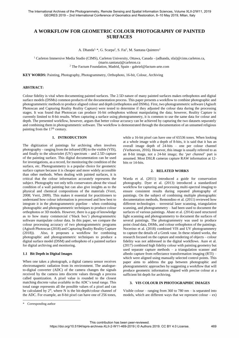
Figure 1 shows the sRGB, Colormatch RGB, Adobe RGB

(1998), ProPhoto RGB, and SWOP CMYK colour spaces

projected onto the 1931 CIE chromacity diagram – a 2D

projection of the XYZ colour model. See Wyszecki and Stiles

(1982), and Verhoeven (2016) for more information on the CIE

colour models.

Figure 1. Colour spaces projected onto the 1931 CIE chromacity

diagram (Wikimedia Commons contributors, 2014)

Dyer et al. (2013) introduced a workflow that uses a Macbeth

colour checker chart, and a uniformly reflective board to correct

images for exposure, colour representation, and inhomogeneous

lighting in VIS photography of painted surfaces They also

present workflows for UV and IR images, but they involve

additional equipment. The proposed workflow uses nip2, which

is a graphical user interface (GUI) for the free image processing

system known as VIPS. The workflow involves five main steps:

1) The RAW images are converted to linear RGB TIFF

images with a depth of 16-bits

2) The 16-bit images are imported into the workspace

made for nip2 – the colour checker image, the uniform

reflective board image, and the image to be corrected

3) The user identifies the 24-colour grid of the colour

checker, and selects the type of correction – ex) colour

and exposure

4) nip2 converts the linear RGB image to the XYZ colour

model, corrects the illumination inhomogeneities,

colour response and exposure and calculates the

average colour error from known values (∆E)

5) The 8 or 16-bit corrected image is exported in the

sRGB colour space

Dyer et al. (2013) recommend using a uniformly reflective board

to correct for inhomogeneous lighting distribution – a technique

known as ‘flat fielding’. However, it is not practical to have a

uniformly reflective board that matches every size of painting

that could be photographed. We use a more widely applicable,

but simplified, flat fielding method that is demonstrated in the

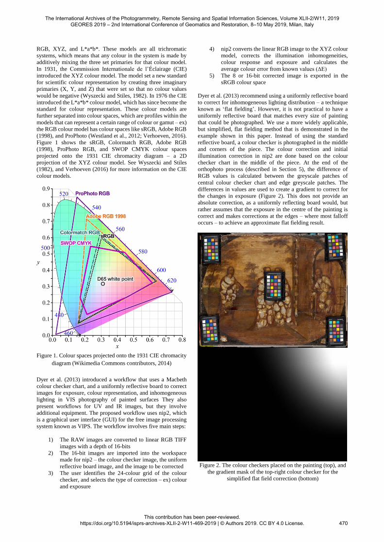
example shown in this paper. Instead of using the standard

reflective board, a colour checker is photographed in the middle

and corners of the piece. The colour correction and initial

illumination correction in nip2 are done based on the colour

checker chart in the middle of the piece. At the end of the

orthophoto process (described in Section 5), the difference of

RGB values is calculated between the greyscale patches of

central colour checker chart and edge greyscale patches. The

differences in values are used to create a gradient to correct for

the changes in exposure (Figure 2). This does not provide an

absolute correction, as a uniformly reflecting board would, but

rather assumes that the exposure in the centre of the painting is

correct and makes corrections at the edges – where most falloff

occurs – to achieve an approximate flat fielding result.

Figure 2. The colour checkers placed on the painting (top), and

the gradient mask of the top-right colour checker for the

simplified flat field correction (bottom)



470

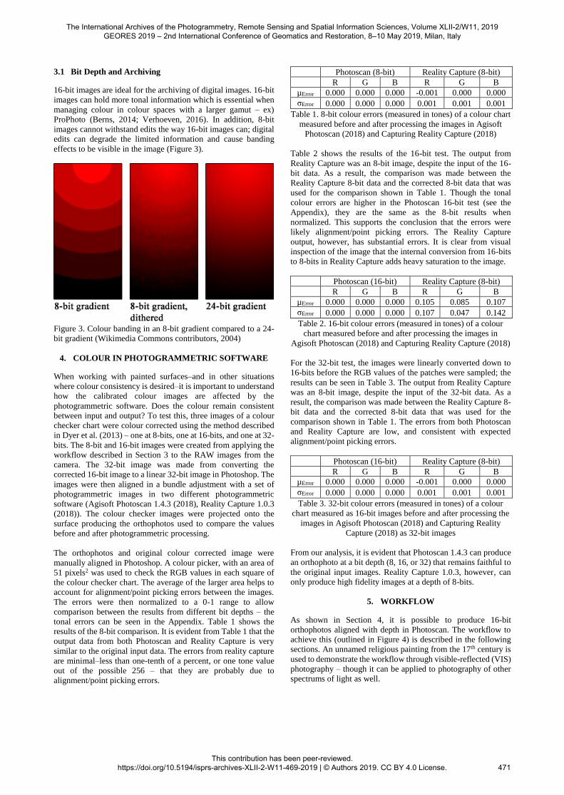
3.1 Bit Depth and Archiving

16-bit images are ideal for the archiving of digital images. 16-bit

images can hold more tonal information which is essential when

managing colour in colour spaces with a larger gamut – ex)

ProPhoto (Berns, 2014; Verhoeven, 2016). In addition, 8-bit

images cannot withstand edits the way 16-bit images can; digital

edits can degrade the limited information and cause banding

effects to be visible in the image (Figure 3).

Figure 3. Colour banding in an 8-bit gradient compared to a 24-

bit gradient (Wikimedia Commons contributors, 2004)

4. COLOUR IN PHOTOGRAMMETRIC SOFTWARE

When working with painted surfaces–and in other situations

where colour consistency is desired–it is important to understand

how the calibrated colour images are affected by the

photogrammetric software. Does the colour remain consistent

between input and output? To test this, three images of a colour

checker chart were colour corrected using the method described

in Dyer et al. (2013) – one at 8-bits, one at 16-bits, and one at 32-

bits. The 8-bit and 16-bit images were created from applying the

workflow described in Section 3 to the RAW images from the

camera. The 32-bit image was made from converting the

corrected 16-bit image to a linear 32-bit image in Photoshop. The

images were then aligned in a bundle adjustment with a set of

photogrammetric images in two different photogrammetric

software (Agisoft Photoscan 1.4.3 (2018), Reality Capture 1.0.3

(2018)). The colour checker images were projected onto the

surface producing the orthophotos used to compare the values

before and after photogrammetric processing.

The orthophotos and original colour corrected image were

manually aligned in Photoshop. A colour picker, with an area of

51 pixels2 was used to check the RGB values in each square of

the colour checker chart. The average of the larger area helps to

account for alignment/point picking errors between the images.

The errors were then normalized to a 0-1 range to allow

comparison between the results from different bit depths – the

tonal errors can be seen in the Appendix. Table 1 shows the

results of the 8-bit comparison. It is evident from Table 1 that the

output data from both Photoscan and Reality Capture is very

similar to the original input data. The errors from reality capture

are minimal–less than one-tenth of a percent, or one tone value

out of the possible 256 – that they are probably due to

alignment/point picking errors.

Photoscan (8-bit) Reality Capture (8-bit)

R G B R G B

µError 0.000 0.000 0.000 -0.001 0.000 0.000

σError 0.000 0.000 0.000 0.001 0.001 0.001

Table 1. 8-bit colour errors (measured in tones) of a colour chart

measured before and after processing the images in Agisoft

Photoscan (2018) and Capturing Reality Capture (2018)

Table 2 shows the results of the 16-bit test. The output from

Reality Capture was an 8-bit image, despite the input of the 16-

bit data. As a result, the comparison was made between the

Reality Capture 8-bit data and the corrected 8-bit data that was

used for the comparison shown in Table 1. Though the tonal

colour errors are higher in the Photoscan 16-bit test (see the

Appendix), they are the same as the 8-bit results when

normalized. This supports the conclusion that the errors were

likely alignment/point picking errors. The Reality Capture

output, however, has substantial errors. It is clear from visual

inspection of the image that the internal conversion from 16-bits

to 8-bits in Reality Capture adds heavy saturation to the image.


R G B R G B

µError 0.000 0.000 0.000 0.105 0.085 0.107

σError 0.000 0.000 0.000 0.107 0.047 0.142

Table 2. 16-bit colour errors (measured in tones) of a colour

chart measured before and after processing the images in

Agisoft Photoscan (2018) and Capturing Reality Capture (2018)

For the 32-bit test, the images were linearly converted down to

16-bits before the RGB values of the patches were sampled; the

results can be seen in Table 3. The output from Reality Capture

was an 8-bit image, despite the input of the 32-bit data. As a

result, the comparison was made between the Reality Capture 8-

bit data and the corrected 8-bit data that was used for the

comparison shown in Table 1. The errors from both Photoscan

and Reality Capture are low, and consistent with expected

alignment/point picking errors.


R G B R G B

µError 0.000 0.000 0.000 -0.001 0.000 0.000

σError 0.000 0.000 0.000 0.001 0.001 0.001


chart measured as 16-bit images before and after processing the

images in Agisoft Photoscan (2018) and Capturing Reality

Capture (2018) as 32-bit images

From our analysis, it is evident that Photoscan 1.4.3 can produce

an orthophoto at a bit depth (8, 16, or 32) that remains faithful to

the original input images. Reality Capture 1.0.3, however, can

only produce high fidelity images at a depth of 8-bits.

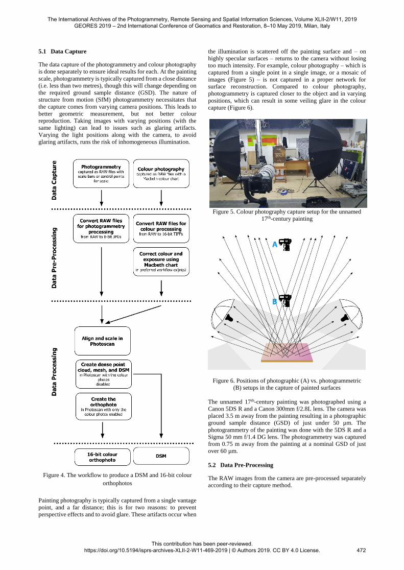
5. WORKFLOW

As shown in Section 4, it is possible to produce 16-bit

orthophotos aligned with depth in Photoscan. The workflow to

achieve this (outlined in Figure 4) is described in the following

sections. An unnamed religious painting from the 17th century is

used to demonstrate the workflow through visible-reflected (VIS)

photography – though it can be applied to photography of other

spectrums of light as well.



471

5.1 Data Capture

The data capture of the photogrammetry and colour photography

is done separately to ensure ideal results for each. At the painting

scale, photogrammetry is typically captured from a close distance

(i.e. less than two metres), though this will change depending on

the required ground sample distance (GSD). The nature of

structure from motion (SfM) photogrammetry necessitates that

the capture comes from varying camera positions. This leads to

better geometric measurement, but not better colour

reproduction. Taking images with varying positions (with the

same lighting) can lead to issues such as glaring artifacts.

Varying the light positions along with the camera, to avoid

glaring artifacts, runs the risk of inhomogeneous illumination.

Figure 4. The workflow to produce a DSM and 16-bit colour

orthophotos

Painting photography is typically captured from a single vantage

point, and a far distance; this is for two reasons: to prevent

perspective effects and to avoid glare. These artifacts occur when

the illumination is scattered off the painting surface and – on

highly specular surfaces – returns to the camera without losing

too much intensity. For example, colour photography – which is

captured from a single point in a single image, or a mosaic of

images (Figure 5) – is not captured in a proper network for

surface reconstruction. Compared to colour photography,

photogrammetry is captured closer to the object and in varying

positions, which can result in some veiling glare in the colour

capture (Figure 6).

Figure 5. Colour photography capture setup for the unnamed

17th-century painting

Figure 6. Positions of photographic (A) vs. photogrammetric

(B) setups in the capture of painted surfaces

The unnamed 17th-century painting was photographed using a

Canon 5DS R and a Canon 300mm f/2.8L lens. The camera was

placed 3.5 m away from the painting resulting in a photographic

ground sample distance (GSD) of just under 50 µm. The

photogrammetry of the painting was done with the 5DS R and a

Sigma 50 mm f/1.4 DG lens. The photogrammetry was captured

from 0.75 m away from the painting at a nominal GSD of just

over 60 µm.

5.2 Data Pre-Processing

The RAW images from the camera are pre-processed separately

according to their capture method.



472

5.2.1 Photogrammetric Images: The photogrammetric

images are converted to high-quality 8-bit JPEG images; the

accuracy of the image colour in these photos is not important

since they are only needed to calculate the geometry of the

subject.

5.2.2 Colour Photography Images: The RAW colour images

are converted to 16-bit TIFF images that are corrected for

exposure, white balance, and colour representation. The colour

photos of the painting were corrected using the method described

in Section 3.

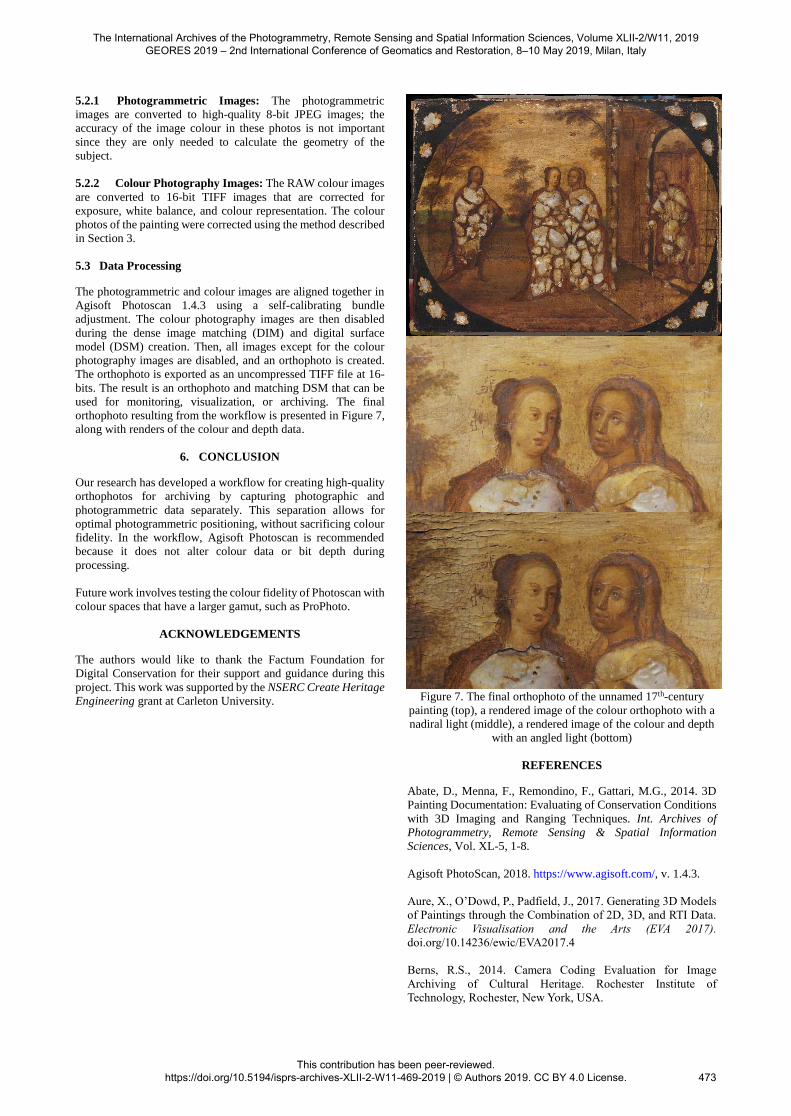
5.3 Data Processing

The photogrammetric and colour images are aligned together in

Agisoft Photoscan 1.4.3 using a self-calibrating bundle

adjustment. The colour photography images are then disabled

during the dense image matching (DIM) and digital surface

model (DSM) creation. Then, all images except for the colour

photography images are disabled, and an orthophoto is created.

The orthophoto is exported as an uncompressed TIFF file at 16-

bits. The result is an orthophoto and matching DSM that can be

used for monitoring, visualization, or archiving. The final

orthophoto resulting from the workflow is presented in Figure 7,

along with renders of the colour and depth data.

6. CONCLUSION

Our research has developed a workflow for creating high-quality

orthophotos for archiving by capturing photographic and

photogrammetric data separately. This separation allows for

optimal photogrammetric positioning, without sacrificing colour

fidelity. In the workflow, Agisoft Photoscan is recommended

because it does not alter colour data or bit depth during

processing.

Future work involves testing the colour fidelity of Photoscan with

colour spaces that have a larger gamut, such as ProPhoto.

ACKNOWLEDGEMENTS

The authors would like to thank the Factum Foundation for

Digital Conservation for their support and guidance during this

project. This work was supported by the NSERC Create Heritage

Engineering grant at Carleton University.

Figure 7. The final orthophoto of the unnamed 17th-century

painting (top), a rendered image of the colour orthophoto with a

nadiral light (middle), a rendered image of the colour and depth

with an angled light (bottom)

REFERENCES

Abate, D., Menna, F., Remondino, F., Gattari, M.G., 2014. 3D

Painting Documentation: Evaluating of Conservation Conditions

with 3D Imaging and Ranging Techniques. Int. Archives of

Photogrammetry, Remote Sensing & Spatial Information

Sciences, Vol. XL-5, 1-8.

Agisoft PhotoScan, 2018. https://www.agisoft.com/, v. 1.4.3.

Aure, X., O’Dowd, P., Padfield, J., 2017. Generating 3D Models

of Paintings through the Combination of 2D, 3D, and RTI Data.

Electronic Visualisation and the Arts (EVA 2017).

doi.org/10.14236/ewic/EVA2017.4

Berns, R.S., 2014. Camera Coding Evaluation for Image

Archiving of Cultural Heritage. Rochester Institute of

Technology, Rochester, New York, USA.



473

https://www.agisoft.com/

https://www.agisoft.com/

Capturing Reality Reality Capture, 2018.

https://www.capturingreality.com/, v. 1.0.3.

Dyer, J., Verri, G., Cupitt, J., 2013. Multispectral Imaging in

Reflectance and Photo-induced Luminescene Modes: A User

Manual. The British Museum, London.

Nocerino, E., Rieke-Zapp, D.H., Tinkl, E., Rosenbauer, R.,

Farella, E. M., Morabito, D., Remondino, F., 2018. Mapping

VIS and UVL Imagery on 3D Geometry for Non-Invasive, Non-

Contact Analysis of a Vase. Int. Archives of Photogrammetry,

Remote Sensing & Spatial Information Sciences, Vol. XLII-2,

773-780.

Remondino, F., Rizzi, A., Barazzetti, L., Scaioni, M., Fassi, F.,

Brumana, R. and Pelagotti, A., 2011. Review of Geometric and

Radiometric Analyses of Paintings. The Photogrammetric

Record, 26(136), 439-461.

Verhoeven, G., 2016. Basics of Photography for Cultural

Heritage Imaging. In: Stylianidis, E., Remondino, F. (Eds.), 3D

Recording, Documentation and Management of Cultural

Heritage. Whittles Publishing, 127-251.

Verri, G., 2008. The use and distribution of Egyptian blue: a

study by visible-induced luminescence imaging. In: K

Uprichard & A Middleton (eds), The Nebamun Wall Paintings.

Archetype, London, pp. 41-50 .

Verri, G., 2009. The spatially resolved characterisation of

Egyptian blue, Han blue and Han purple by photo-induced

luminescence digital imaging. In: Analytical and Bioanalytical

Chemistry, Vol 394(4), pp. 1011-1021.

https://doi.org/10.1007/s00216-009-2693-0

Warda, J. (Editor), Frey, F., Dawn Heller, D., Kushel, D.,

Vitale, T., Weaver, G., 2011. The AIC Guide to Digital

Photography and Conservation Documentation, Third Edition.

American Institute for Conservation of Historic and Artistic

Works, Washington, D.C..

Westland, S., Ripamonti, C., Cheung, V., 2012. Computational

Colour Science Using MATLAB, 2nd Edition. Wiley, Sussex, 4-

11.

Wikimedia Commons contributors, 2004. Colour banding

example01.png. Wikimedia Commons, the free media

repository,

https://commons.wikimedia.org/w/index.php?title=File:Colour_

banding_example01.png&oldid=129798746 (Last accessed

March, 2019).

Wikimedia Commons contributors, 2014. CIE1931xy gamut

comparison.svg. Wikimedia Commons, the free media

repository,

https://commons.wikimedia.org/w/index.php?title=File:CIE193

1xy_gamut_comparison.svg&oldid=324046804 (Last accessed

March, 2019).

Wyszecki, G., Stiles, W.S., 1982. Color Science: Concepts and

Methods, Quantitative Data and Formulae. Wiley, New York,

228-320.

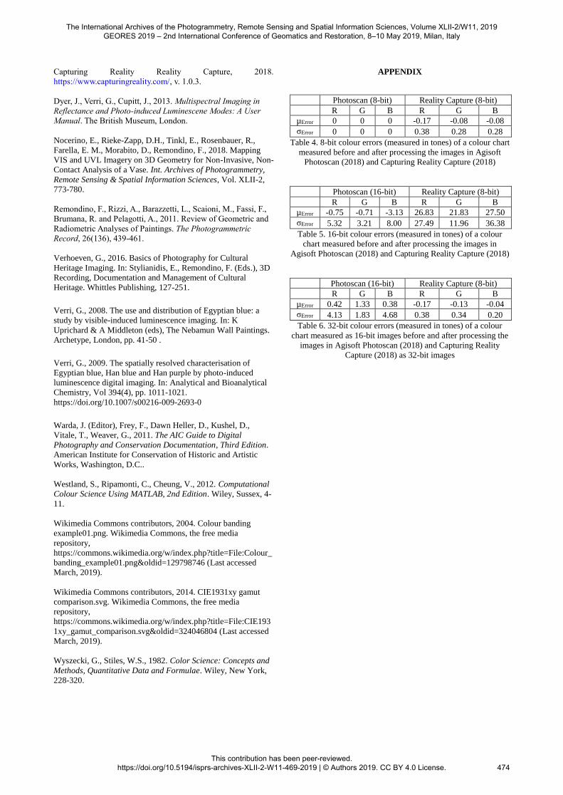
APPENDIX


R G B R G B

µError 0 0 0 -0.17 -0.08 -0.08

σError 0 0 0 0.38 0.28 0.28

Table 4. 8-bit colour errors (measured in tones) of a colour chart

measured before and after processing the images in Agisoft

Photoscan (2018) and Capturing Reality Capture (2018)


R G B R G B

µError -0.75 -0.71 -3.13 26.83 21.83 27.50

σError 5.32 3.21 8.00 27.49 11.96 36.38


chart measured before and after processing the images in

Agisoft Photoscan (2018) and Capturing Reality Capture (2018)


R G B R G B

µError 0.42 1.33 0.38 -0.17 -0.13 -0.04

σError 4.13 1.83 4.68 0.38 0.34 0.20


chart measured as 16-bit images before and after processing the

images in Agisoft Photoscan (2018) and Capturing Reality

Capture (2018) as 32-bit images



474

https://www.capturingreality.com/

https://www.capturingreality.com/

Documents

A WORKFLOW FOR GEOMETRIC COLOUR PHOTOGRAPHY OF … · 2019-05-05 · orthophoto process (described in Section 5), the difference of RGB values is calculated between the greyscale