IEEE TRANSACTIONS ON MICROWAVE THEORY AND TECHNIQUES, VOL. 43, NO. 8, AUGUST 1995 1961

A Wiener-Hopf-Type Analysis of Microstrips Printed on Uniaxial Substrates: Effects

of the Substrate Thickness George A. Kyriacou, Member, IEEE, and John N. Sahalos, Senior Member, IEEE

Abstract-A Wiener-Hopf-type analysis of the canonical prob- lem of a TEM wave obliquely incident at the edge of the truncated upper conductor of a parallel plate waveguide loaded with a uniaxial anisotropic dielectric is presented. A numerical inte- gration scheme as well as a thin substrate approximation for the reflection coefficient is given. The influence of the dielectric anisotropy and the slab thickness on the reflection coefficient and the edge admittance are investigated. Numerical results show the importance of the dielectric anisotropy and the expected effects in microstrip applications.

I. INTRODUCTION

LOT OF substrate materials used in the fabrication of A microstrip lines or patch antennas exhibit a dielectric anisotropy. The anisotropy is either intrinsic of the material or artificially caused by the substrate manufacturing process. Moreover, crystalline substrates are preferable in some appli- cations because they have certain advantages over ceramics, such as higher homogeneity, lower losses, and lower varia- tions from sample to sample. Examples of monocrystalline dielectrics suggested for use as substrates include: monocrys- talline sapphire, with relative permittivity along the principal crystal axis E ~ I =11.6, and perpendicular to that EL =9.4 and monocrystalline magnesium fluoride with E I ~ =4.826 and E L =S.S. Ceramic Impregnated teflon, like Epsilam 10 with ~ l l =10.2 and E L =13.0, is an example of artificially caused uniaxial anisotropy. The substrate anisotropy must be taken into account because it can be used to improve the performance of printed lines and antennas.

Although many studies have been presented on transmission lines (see an excellent review article written by Alexopoulos [ 11 and the references therein), there are rather few works (e.g., [2]-[4], [ 121) in the field of antennas. Also, some recent works are studying the characterization of microstrip discontinuities patterned on uniaxial anisotropic substrates (e.g., [ 131). At the same time the interest of the investigators is extending toward the inclusion of an also uniaxial superstrate [ 141, [ 151. In our previous study [4], the Wiener-Hopf technique has been applied to solve the canonical problem of a TEM wave obliquely incident on the truncation of the upper plate of a parallel plate waveguide loaded with a uniaxially anisotropic

Manuscript received November IO, 1994; revised April 24, 1995. G. A. Kyriacou is with the Department of Electrical Engineering, Demokri-

I. N. Sahalos is with the Department of Physics, University of Thessaloniki,

IEEE Log Number 9412676.

tos University of Thrace, 67100 Xanthi, Greece.

54006 Thessaloniki, Greece.

dielectric slab. Moreover, the integrals arising from the solu- tion of the Wiener-Hopf equations have been approximated in closed form for the usual case of electrically thin substrates. This work, [4], could be considered as an extension of the studies by Kuester and Chang [5], [6]. The validity of [4] has been tested in two ways. First, letting the anisotropy ratio be equal to one (or € 1 1 = E L = E ~ ) . It was verified that the infinite integrals and the closed form expressions were exactly reduced to the corresponding ones of the isotropic problem [SI, [6]. Second, by comparing the numerical results for the resonant frequency of rectangular patch antennas with those given by Nelson [3] and Pozar [2]. It was found that they were in very good agreement.

Our present effort has to do with the numerical evaluation of the infinite Sommerfeld-type integrals involved in the field expressions and the application of the theory in the analysis of microstrip antennas. The numerical integration will show the limits of the thin substrate approximation and will help investigate new applications with electrically thick substrates.

In order for this paper to be self-sustained, we first summa- rize the formulation given in [4].

11. FORMULATION OF THE WIENER-HOPF EQUATIONS FOR THE UNIAXIAL SUBSTRATE

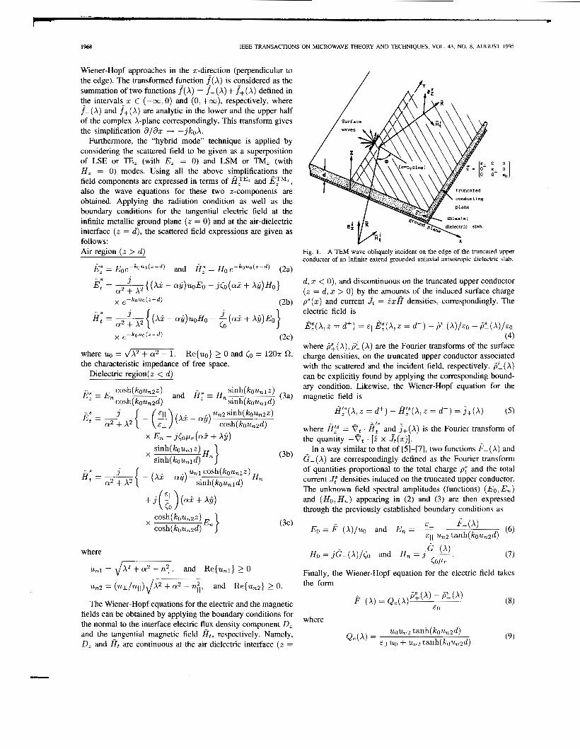
Consider a vertically polarized TEM wave obliquely in- cident (at an angle @) on the edge of the truncated upper conductor of an otherwise infinite parallel plate waveguide loaded with an infinitely extended uniaxial dielectric slab (see Fig. 1). The uniaxial dielectric is assumed to be fabricated (or cut) with its optical axis perpendicular to the conductor plane (along the z-axis). Let the relative dielectric constant along the optical axis be E , = € 1 1 and the one transverse to the optical axis be E, = cy = EL. The corresponding refraction indices are nil = and n1 = m. The vertically polarized TEM wave can be expressed as E4 = exp[jko(<s - cry)], where (Y = n11 sinp, < = lzll cosp and ko is the wavenumber in free space. The scattered field (reflected and radiated) by the edge can be obtained with the adoption of the continuous Fourier spectrum in conjunction with the Wiener-Hopf technique.

In order to get an analytical solution, Maxwell equations are first simplified by considering: 1) time harmonic fields of the form ,jut, 2) propagation of the incident and scattered field in the y-direction, as e - j k o a y , which gives d ldy + -jkocu, and 3) typical Fourier transform pair { f (A) , f(s)} used in

00 18-9480/95$04.00 0 1995 IEEE

IEEE TRANSACTIONS ON MICROWAVE THEORY AND TECHNIQUES. VOL. 43, NO. 8, AUGUST 1995

Wiener-Hopf approaches in the x-direction (perpendicular to the edge). The transformed function f ( A ) is considered as the summation of two functions f( A) = f- (A) + f+ (A) defined in the intervals x E (-00~0) and (0, +m), respectively, where f- (A) and f+ (A) are analytic in the lower and the upper half of the complex A-plane correspondingly. This transform gives the simplification d/dx + - j k o A .

Furthermore, the "hybrid mode" technique is applied by considering the scattered field to be given as a superposition of LSE or TE, (with E, = 0) and LSM or TM, (with H , = 0) modes. Using all the above simplifications the field components are expressed in terms of ,TEz and ETMz, also the wave equations for these two z-components are obtained. Applying the radiation condition as well as the boundary conditions for the tangential electric field at the infinite metallic ground plane ( z = 0) and at the air-dielectric interface ( z = d) , the scattered field expressions are given as follows: Air region ( z > d )

E: = E,e-buO("-d) and fiz = H , e--kOuO(z--d) (2a)

E" - ' { ( A i - a$)uoEo - j C 0 ( ~ i + Ajj)Ho} - cy2 + A2

j ff + A (0

kj = A{ ( A i - c ~ $ ) u ~ H ~ - -(ai + A$)Eo

the characteristic impedance of free space. Dielectric region(z < d )

X

where

un1 = dAz + cy2 - n:, and Re{u,l} 2 0

un2 = ( n ~ / q ) \ / A ~ + a2 - n t ,

The Wiener-Hopf equations for the electric and the magnetic fields can be obtained by applying the boundary conditions for the normal to the interface electric flux density component D, and the tangential magnetic field H,, respectively. Namely, D, and Ht are continuous at the air dielectric interface ( z =

and Re{u,2} 2 0.

Fig. I. A TEM wave obliquely incident on the edge of the truncated upper conductor of an infinite extend grounded uniaxial anisotropic dielectric slab.

d, x < 0), and discontinuous on the truncated upper conductor ( z = d ,x > 0) by the amounts of the induced surface charge p" (z ) and current jt = i x H densities, correspondingly. The electric field is

E p , z = d+) = &,lE:(A,a = d - ) - p y x ) / € , +&(A)/€, (4)

where 3; (A), pZ- (A) are the Fourier transforms of the surface charge densities, on the truncated upper conductor associated with the scattered and the incident field, respectively. pZ-(A) can be explicitly found by applying the corresponding bound- ary condition. Likewise, the Wiener-Hopf equation for the magnetic field is

( 5 ) ,;(A, z = d f ) - ,;(A, z = d - ) = j + ( A )

where fi; = V, . k; and j + ( A ) is the Fourier transform of the quantity -0, . [i x Jt(z)] .

In a way similar to that of [5]-[7], two functions F - ( A ) and G- (A) are correspondingly defined as the Fourier transform of quantities proportional to the total charge p: and the total current J f densities induced on the truncated upper conductor. The unknown field spectral amplitudes (functions) (Eo, E,) and (Ho, H,) appearing in (2) and (3) are then expressed through the previously established boundary conditions as

G - ( A ) HO = j G - ( A ) / C o and H , = j-. (OPL,. (7)

Finally, the Wiener-Hopf equation for the electric field takes the form

where

”.. - t ’1

KYRIACOU AND SAHALOS: A WIENER-HOPF-TYPE ANALYSIS OF MICROSTRIPS 1969

while, that for the magnetic field

where

For the solution of the Wiener-Hopf equations it is necessary to perform a factorization of the functions Qe(A) and Qm(A) into a product Q+(X)Q-(A), where &+(A) is a “positive” and Q-(A) is a “negative” function, in the sense that they are analytic in the upper and lower complex A-half planes. The factorization technique, given by Mittra and Lee [8], helps to find a solution of the following form:

~ - ( x ) = -jkod Jz X + j a tanh(A) 7r ‘ I { , / w - j a t a n h ( A )

where

€ 1 2 ~ 0 tanh(kou,zd)[~~uo + uni coth(kou,id)] { ~ , , Z [ E L U O + u,2 t a n h ( k o u d ) ] dA

A2 + a2’ x- (15c)

In order for the above integrals to have an efficient numerical convergence, the argument of the natural logarithm should approach unity as the integration variable (A) goes to infinity.

This is actually true for all of them except A ( a ) [see 15(c)] which, in order to satisfy these conditions, is modified to

dA A2 + a2

x-

From the above expressions all the components of the electric and magnetic fields can be obtained through the functions I? (A) and G- (A) in the Fourier spectrum domain. An inverse Fourier transform is needed to get their expressions in the real space domain. This is a quite complicated task, since the field spectral components are already expressed as Sommerfeld type integrals.

Near the edge, higher-order modes are excited, but most of them are evanescent type modes and they vanish at a practically small distance. Therefore, only the propagating modes will exist at some distance from the edge. The dominant mode which always exists is again a vertically polarized TEM- reflected wave. This wave can be obtained with the help of a reflection coefficient, as

= j7r F-(A = 4-1 - - , j X ( a ) (16) ko d d F

where X ( a ) after some algebraic manipulations turn out to be

The contribution of the integral involved in the f e ( A ) expres- sion at the pole w + X = + JF a is extracted and fe is expressed as a principal value integral more properly suited for numerical integration (since the pole singularity is extracted). That is

where for convenience the integration variable is changed from w :o A.

It is important to note that, by letting the anisotropy ratio equal to one, namely n l = 1211 = n or EL = E I I = E ~ , the expressions, either for the field components or the Wiener- Hopf equations solution, are exactly reduced to those of the isotropic case given by Chang and Kuester [ 5 ] .

~.. r - I970 IEEE TRANSACTIONS ON MICROWAVE THEORY AND TECHNIQUES, VOL 43, NO. 8, AUGUST 1995

The TEM reflection coefficient can be calculated either by using numerical integration or the thin substrate approx- imation. With the knowledge of r T E M the open end edge admittance Ye can be evaluated

1 - e j X ( a ) yo + = -jyo t a n ( X ( f f ) ) . (19) - -

G,, Be are the edge conductance and edge susceptance, re- spectively. YO is the characteristic admittance of the parallel plate waveguide ioaded with a uniaxial dielectric slab. The ad- mittance YO, related to the 2-polarized TEM wave propagating in this waveguide, can be defined as the ratio of the current per unit length flowing on the conductors in the direction of propagation to the voltage developed between them. Using for simplicity the incident TEM wave components (the same result can be obtained from the scattered TEM wave), it is found that yo = IH; I / (E ld ) or yo = n l l / ( P d o d ) .

111. SURFACE WAVES, CUTOFF FREQUENCIES, AND APPROXIMATE WAVENUMBERS

The LSE and LSM surface wave characteristic equations can be obtained by setting, respectively the denominators of Q, and Qm in (9) and (1 1) equal to zero. In order to determine their cutoff frequencies or the modes’ turn on conditions, a clarifying “graphical” solution of such transcendental equa- tions, used by many authors, e.g. [lo], is applied. For the LSE modes, let us define their wavenumber a as a;e = X2 + CY’, and let 4- = k,,/ko, ,/e = h,/lco, un2 =

j (n~/n11) . k,,/Ic~ and uo = h,/ko. Using these definitions the LSE modes characteristic equation becomes

Also the unknowns k,, and he are simply related as

The above two equations must be solved simultaneously. Re- arranging, we get a form more suitable for graphical solution

(204

In order to get a graphical representation (20c) and (20d) can be plotted (see [lo] for the isotropic case) on an axis system k,,d( n~ /nil ) versus h,d( n l /nil ). Equation (20d) represents a circle about the origin with radius T,. Moreover, recalling the restriction Re(u0) 2 0, the valid solutions (points where the two curves intercept each other) are only those giving he 2 0. Since the curve of (20c) passes always through the origin and is lying on the positke half plane, there is always a valid first-order solution. This solution corresponds to the first LSE mode, which is then always excited. Furthermore, as the

radius T, becomes larger (thicker substrate kod /” or larger anisotropy ratio (n l ln l l ) /), higher order LSE modes are excited. Valid solutions (he 2 0) are obtained for T , 2 p e r . The turn on condition of the p,th mode is defined as T, = p e r , which gives

k o d s J v = p e r with p , = 0, 1 , 2 , . . . (21a) nI I

with a cutoff frequency

f c , p , = ..e/{ 2 d z Jv} (21b)

c is the free space light velocity. The LSM modes excitation can also be examined in a

similar manner. Consider the wavenumber to be apm, defined as a:, = X2+a2 and ,/= = k, , /k~, d G =

The LSM characteristic equation along with the relation between IC,, and h, result in the following two simultaneous transcendental equations

h m / h , un1 = jkcm/ko and uo = h m / h .

- (kcmd) cot (kcmd) = p r ( h m d ) (22a)

(kc,d)2 + ( h m d ) 2 = kod n t - = ~ f . (22b) ( J-7 The above equations can be graphically examined by plotting them in a h,d versus k,,d system. Again we have to recall the restriction Re(u0) 2 0, which means that valid solutions must satisfy h, 2 0. This condition can only be met when the radius of the circle (about the origin) defined by (22b) becomes larger than r / 2 , namely T, 2 r / 2 . This fact gives the important result that there isn’t any LSM surface wave excitation until the slab thickness becomes thick so that T, 2 r / 2 . When the slab thickness increases even more, there is a possibility for higher-order LSM mode excitations. Their turn on condition is T, 2 (2q , - 1)r /2 , where qm is the LSM mode order. This mode can be expressed as

od nL - 1 2 (2q, - l ) r / 2 where qm = 1 , 2 , 3 , . . . (23)

k F

The corresponding cutoff frequencies can then defined as

fc, qm = (2qm - I)./ { 4 d JG}. (24)

For the first LSM mode the cutoff frequency can be expressed in prescribed units as fc,LSM1(GHz) = 75/ { d( mm) d m } .

Even more interesting expressions are the first LSM and the second LSE modes turn on conditions in terms of the normalized slab thickness d/X

LSMl turn on: d/X = l / { 4 J G } (25a)

LSE2 turn on: d/X = I/{ 2: Jv}. (25b)

For example, considering a non-magnetic dielectric slab, the LSMl turn on condition for E~ =9.6 is d/X 20.085 and for

~~

I ~~

KYRIACOU AND SAHALOS. A WIENER-HOPF-TYPE ANALYSIS OF MICROSTRIPS 1971

€1 =13 is d/X 20.072. Also, if €1 =13 and € 1 1 =10.2 the LSE2 turn on condition is d / X 20.146.

Summarizing, we can say that the first LSE mode is always excited. With an increase in the slab thickness, usually the first LSM can be turned on, followed by the second LSE mode.

During the numerical integration for the calculation of either the scattered field components or just the TEM reflection coefficient, the exact location of the surface wave poles ape and apm is always needed. The most convenient manner to solve the characteristic equations is the use of iterative schemes, like the Newton-Raphson. These schemes always need a suitable starting value for the root to achieve fast convergence. For this reason the first mode wavenumbers are estimated by using the electrically thin substrate (kod << 1) approximation, which gives

The corresponding expression for the first LSM mode is

Of course, before attempting to solve for the roots, we first have to check if the corresponding turn on condition has been established.

IV. A THIN SUBSTRATE APPROXIMATION

The electrically thin substrate (kod << 1) is often encoun- tered in practical applications. Moreover, in applications such as wide microstrip lines and patch antennas the characteristic equations for the effective dielectric constant, the resonant fre- quency and the input impedance involve the above-developed reflection coefficient with multiple arguments. Therefore, the calculation of r T E M must be effective and fast, which means that it cannot be achieved using numerical integration. So, a thin substrate approximation, in a manner similar to that of Kuester et al. [6], using a Mellin transform, is important. The closed form expressions obtained for the two integrals A ( c Y ) and fe(a) are given in [4].

In the general case of electrically thick substrate or when more accurate results are needed, this thin substrate approx- imation can be used as a first step in the solution of patch antennas transverse resonance characteristic equations.

v. INTEGRATION PATH AND EFFECTS OF SINGULARITY LOCATIONS

A numerical integration scheme to calculate the TEM reflec- tion coefficient as a function of the substrate thickness is used. The involved integrals to be evaluated numerically are A(a) and f e ( - , / F ) , which appear in (15d) and (18). First, the integrand singularities must be defined and the integration contour must then be properly deformed to avoid them.

Both integrands possess a pair of branch cuts at uo = 0 or X = * j d n as well as a set of LSE poles at

where ape is the corresponding

LSE mode wavenumber obtained from the solution of their characteristic equation. For the substrate thickness usually used in practical applications, only the first LSE mode is excited. The corresponding wavenumber ape 1 is calculated from the solution of the characteristic equation with a lop6 error tolerance by using a Newton-Raphson technique.

The contribution of the pole located at X = JF to the f, integral, has already been taken into account in (1 8) as a Cauchy principal value. For this last approach we have to keep in mind that an integration path along the real X-axis is assumed. Also, we must take into account that the substrate is considered to be lossless, so that this pole lies on the real axis, otherwise it will be shifted to the lower complex A-half plane.

Additionally, the integrand of the function A ( c Y ) possess a pair of simple poles on the Im(X) axis at X = &ja. Moreover, if the substrate is thick enough then a set of LSM poles will also appear on the real axis at X = fX, = 4=4-. Usually in practice none LSM mode is excited and only for quite thick substrates just the first one is turned on, according to the condition (23).

Furthermore, some terms are not singular (removable singu- larities) but they may cause numerical instabilities if they are not properly accounted for. Thus, in both integrands the term “tanh(koduL,2)/u,2” in the limit when u,2 -+ 0, must be replaced by its limiting value kod. Similarly, the f , integrand term u,1 . coth(kadunl) at the limit unl --+ 0 is replaced by

It is obvious that the location of the above singularities depends upon the value of the propagation constant along the y-axis Q = 1211 sin(p), where cp is the angle of incidence. Considering the usual practical case where the slab thickness is such that only LSEl is excited and keeping in mind that always ape 1 > 1. We distinguish three cases for the singularity locations.

l/kod.

First case aP,l < Q < 71.11: All singularities, except that of the f? pole at X = ,/F, are located on the Im(X) axis. Since, it is CY > 1,uo is purely real. From (2) we can see that the electromagnetic field in the air region decays exponentially, which means that there isn’t any “sky wave radiation.” Also, it has been proved by Chang et al. [5], that the surface wave propagating in the dielectric away from the open edge (area without upper conductor, negative 2-direction) behaves as exp(k0 a2 - a2 2 ) . So, for the case CY > CY^,^, it decays exponentially as it propagates away from the edge. Moreover, as can be seen in the next section, X ( a ) is real and consequently, the reflection coefficient magni- tude becomes unity. This phenomenon corresponds to a total reflection and can be utilized to guide electromag- netic waves in the y-direction. Such an application is the study of wide microstrip lines. Second case 1 < CY < ap,l < 1211: Again there is no sky wave radiation since uo remains purely real and the corresponding branch cut lies on the Im(X) axis. The surface wave pole is moved on the Re( A) axis and

J--

1972 IEEE TRANSACTIONS ON MICROWAVE THEORY AND TECHNIQUES, VOL. 43, NO. 8, AUGUST 1995

A 0

#

(b)

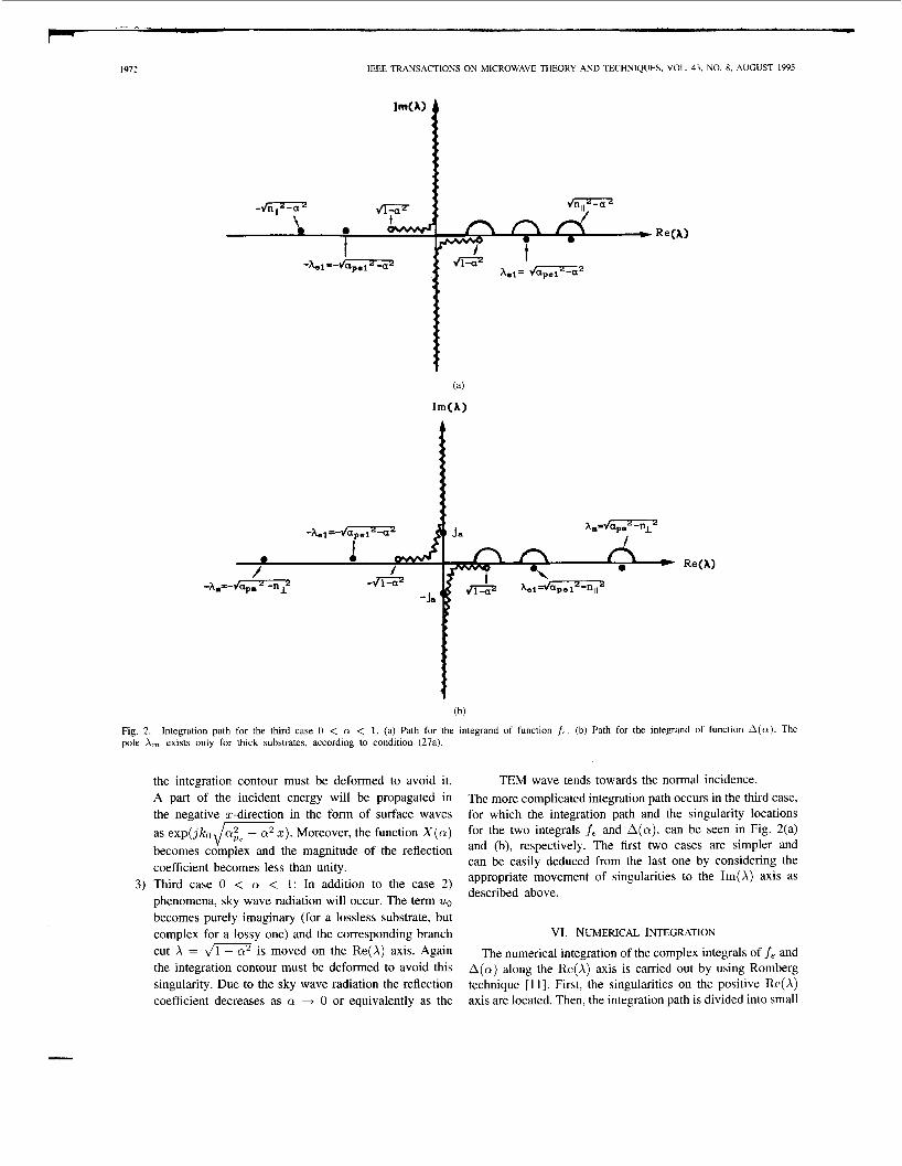
Fig. 2. pole A, exists only for thick substrates, according to condition (27a).

Integration path for the third case 0 < n < 1. (a) Path for the integrand of function f<. (b) Path for the integrand of function ~ ( c u ) . The

the integration contour must be deformed to avoid it. A part of the incident energy will be propagated in the negative z-direction in the form of surface waves as exp(jk0 , / w z ) . Moreover, the function X ( a ) becomes complex and the magnitude of the reflection coefficient becomes less than unity.

3 ) Third case 0 < Q < 1: In addition to the case 2 ) phenomena, sky wave radiation will occur. The term uo becomes purely imaginary (for a lossless substrate, but complex for a lossy one) and the corresponding branch cut X = d m is moved on the Re(X) axis. Again the integration contour must be deformed to avoid this singularity. Due to the sky wave radiation the reflection coefficient decreases as (Y + 0 or equivalently as the

TEM wave tends towards the normal incidence. The more complicated integration path occurs in the third case, for which the integration path and the singularity locations for the two integrals fe and A(a) , can be seen in Fig. 2(a) and (b), respectively. The first two cases are simpler and can be easily deduced from the last one by considering the appropriate movement of singularities to the Im(X) axis as described above.

VI. NUMERICAL INTEGRATION

The numerical integration of the complex integrals of f e and A(a) along the Re(A) axis is carried out by using Romberg technique [ 1 11. First, the singularities on the positive Re( A) axis are located. Then, the integration path is divided into small

r- KYRIACOU AND SAHALOS: A WIENER-HOPF-TYPE ANALYSIS OF MICROSTRIPS

/ - 4-18.2 - 4-13.8 - 4-6.8

1973

2-10.2 2-10.2 2-10.2

sections, especially on the neighborhood of the singularities. An adaptive Romberg integration is applied to each of these finite intervals with a lou6 error tolerance. The integration is performed upto a point close to the singularity and continues from a point just after the singularity. Logarithmic singularities can be approached easier and more closely, because of the slowly varying nature of the logarithm. Considering to be such a logarithmic singularity, the interval on one side is taken within the points 0.9A0 and (1 - 10-5)X~ and the integration resumes on the other side from the point (1 + 10-5)X0 to 1.lX0 and continues. On the other hand, functions are varying very fast at pole singularities, like fe at the pole A, = dw. So, this pole must be approached gradually, while at the same time its location must be “exactly” determined. In the scheme used, A, is approached by intervals defined by the points 0.8A,,0.99Xp and 0.9999X, on one side and by l .OOOIXp, l . O I X p and 1.2X, on the other side. In this manner the pole is approached to and as we previously mentioned its location is estimated with a lop6 tolerance. Also, the contribution on the pole itself is taken as a Cauchy principal value. Finally, some more intervals are taken as fractions of the [0, max(n1, nil)] where the integrals contribution is expected to be more significant.

For the semi-infinite interval well beyond the singularities, a progressive Romberg integration is used. Namely, integration is performed on subintervals of length l/kod, until the last subinterval contribution is less than IOp5.

Even though the integration technique described in the last two sections refers to a lossless substrate, it can also be applied to lossy ones.

VII. NUMERICAL RESULTS AND DISCUSSIONS

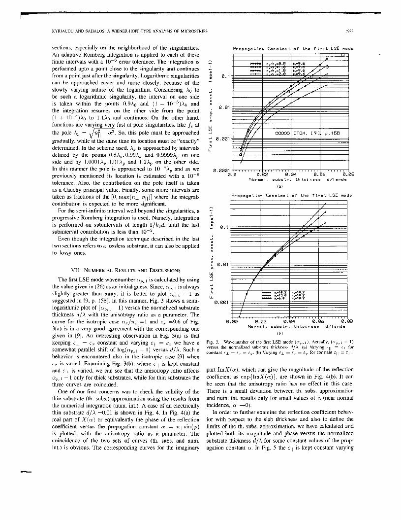
The first LSE mode wavenumber cy,, 1 is calculated by using the value given in (26) as an initial guess. Since, c y p , 1 is always slightly greater than unity, it is better to plot ap,l - 1 as suggested in [9, p. 1.581. In this manner, Fig. 3 shows a semi- logarithmic plot of ( c y p e 1 - 1) versus the normalized substrate thickness d/X with the anisotropy ratio as a parameter. The curve for the isotropic case n,/n, =1 and E, =9.6 of Fig. 3(a) is in a very good agreement with the corresponding one given in [9]. An interesting observation in Fig. 3(a) is that keeping E L = E, constant and varying E I I = E, we have a somewhat parallel shift of log(apel - 1) versus d/A. Such a behavior is encountered also in the isotropic case [9] when E, is varied. Examining Fig. 3(b), where ~ l l is kept constant and E L is varied, we can see that the anisotropy ratio affects c y p , 1 - 1 only for thick substrates, while for thin substrates the three curves are coincided.

One of our first concerns was to check the validity of the thin substrate (th. subs.) approximation using the results from the numerical integration (num. int.). A case of an electrically thin substrate d/X =0.01 is shown in Fig. 4. In Fig. 4(a) the real part of X(a) or equivalently the phase of the reflection coefficient versus the propagation constant cy = 7211 sin(cp) is plotted, with the anisotropy ratio as a parameter. The coincidence of the two sets of curves (th. subs. and num. int.) is obvious. The corresponding curves for the imaginary

P r o p a g o t t o n C o n s t a n t o f t h e f l r s t LSE mode

I I I I V I - 7

I - m : 0.1 v

3

c m 0 0 . 0.01 n

n w v) -J

0 L

3 0 L d

IL

0.001

0.0001 0.0 0.02 0.04 0.06 0.08

Norma I . s u b s tr , t h lck n e s s d / l amda

(a)

P r o p a g o t t o n C o n s t a n t o f t h e f t r s t LSE mode

n a Y

3 0 C 0 0

n

n w v) -I

0 L

0.1

0.01

e) I / I I I 0

LL L d

0. 00 1

0.00 0.02 0.04 0.06 0.08 N o r m a l . e u b s t r . t h l c t n e s s d / l o m d o

(b)

Fig. 3. Wavenumber of the first LSE mode ( m P , 1 ). Actually, (nPei - 1) versus the normalized substrate thickness d / A . (a) Varying E I I = E ; for constant E= = E~ = c y . (b) Varying EL = = sy for constant E I I = E = .

part ImX(a ) , which can give the magnitude of the reflection coefficient as exp{ImX(a)}, are shown in Fig. 4(b). It can be seen that the anisotropy ratio has no effect in this case. There is a small deviation between th. subs. approximation and num. int. results only for small values of cy (near normal incidence, cy +O).

In order to further examine the reflection coefficient behav- ior with respect to the slab thickness and also to define the limits of the th. subs. approximation, we have calculated and plotted both its magnitude and phase versus the normalized substrate thickness d/X for some constant values of the prop- agation constant a. In Fig. 5 the ~ l l is kept constant varying

r

1974 IEEE TRANSACTIONS ON MICROWAVE THEORY AND TECHNIQUES, VOL. 43, NO. 8, AUGUST 1995

R e f I e c t t o n

Norm. s u b s t r . t h t c t . d/lamdo=8.01, F r e q . f=3GHz

c o e f f IC ten t Gamma=eJx*) sol I d I l n e : T h l n s u b s t r o t e o p p r o x . d t s c r e t e s y m b o l s : Numer l c o l I n t s g a t Lon

1.50

1 .OO

h A

a 5 0.50 d

0.00

0

sol I d I t n e : T h l n s u b s t r a t e o p p r o x . d l s c r e t e s y m b o l s : N u m e r l c o l I n t e g r o t l o n

Norm. S u b s tr. t h l c t . d / l omda=0.01, F r e q . f=3GHz 0.03 I 0.02

0.02 h - 0 5 0.01 E +I

0.01

0.00

I I I I 0.00 1 .OO 2.00 3.00 4.00

P r o p . c o n s t . o = n ( p o r o l . ) * s l n ( p h l )

(b)

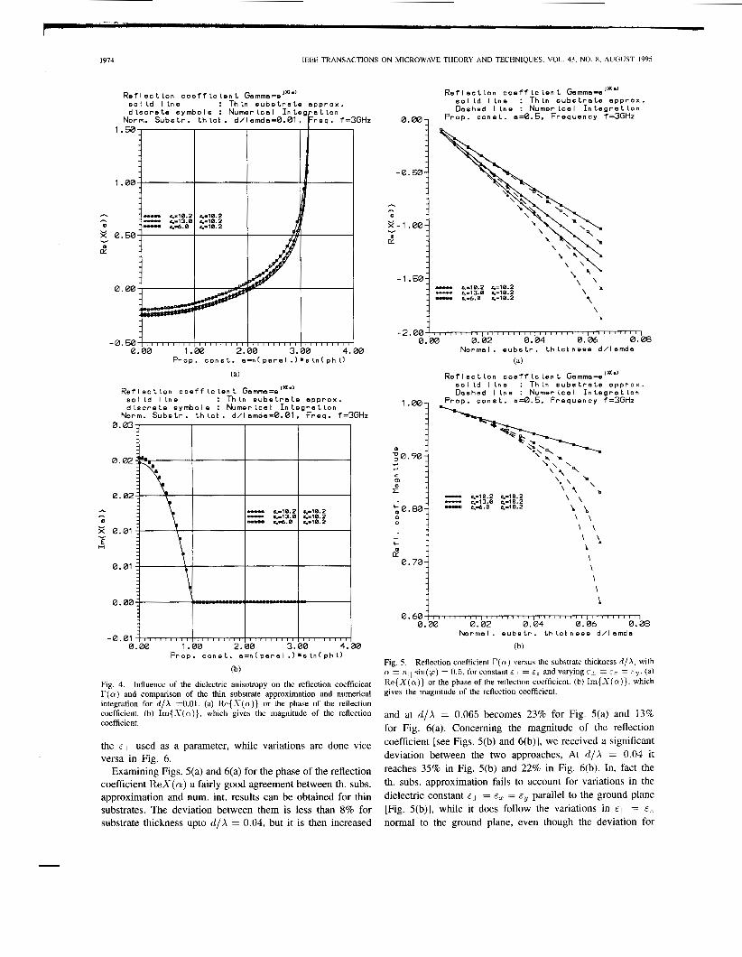
Fig. 4. Influence of the dielectric anisotropy on the reflection coefficient T ( a ) and comparison of the thin substrate approximation and numerical integration for d/X =0.01. (a) R e { X ( a ) } or the phase of the reflection coefficient. (b) Im(X(cy)}, which gives the magnitude of the reflection coefficient.

the E L used as a parameter, while variations are done vice versa in Fig. 6.

Examining Figs. 5(a) and 6(a) for the phase of the reflection coefficient R e X ( a ) a fairly good agreement between th. subs. approximation and num. int. results can be obtained for thin substrates. The deviation between them is less than 8% for substrate thickness upto d/X = 0.04, but it is then increased

R e f I e c t l o n c o e f f IC t e n t Gamma=e’X’) s o l I d I l n e : T h t n s u b s t r a t e a p p r o x . D a s h e d I t n e : Numer t c a l I n t e g r o t l o n

P r o p . c o n s t . a=0.5. F r e q u e n c y f=3GHz

1 -0.50

h

v 5-1 .OO B

\ \ \> \ ‘ \ b

\

- 4-10.2 4-10.2 - 4-6.8 4-10.2 - 4-13.0 q-10.2

-1.50

\ b

-2.00: I 1 1 1 1 1 1 1 1 ~ 1 1 , I I I I I I I I I I I I I I I 0.06 I , I I I I I I I I 0.08 I 1

0.00 0.02 0.04 N o r m a l . s u b s t r . t h l c t n e s s d / l o m d a

1*001 (a)

R e f I e c t t o n c o e f f IC t e n t Gamma=e”” s o l I d I t n e : T h l n s u b s t r a t e o p p r o x . D a s h e d I \ n e : N u m e r l c a l I n t e g r o t l o n

P r o p . c o n s t . a=0.5. F r e q u e n c y f=3GHz

B 0.70

\ \

k \ \

\ \a

1 , , , , , , , , , , , , , , , ( , , I , , , , ( , , , , I(! , , , , I , , I

0.60 0.00 0.02 0.04 0.06 0.08

N o r m a l . s u b s t r . t h l c t n e s s d / l amda

(b)

Fig. 5. Reflection coefficient I?(@) versus the substrate thickness d / A , with a = R I I sin(cp) = 0.5, for constant € 1 1 = c z and varying E L = = c y . (a) R e { X ( a ) } or the phase of the reflection coefficient. (b) Im{X(cy)}, which gives the magnitude of the reflection coefficient.

and at d / X = 0.065 becomes 23% for Fig. 5(a) and 13% for Fig. 6(a). Concerning the magnitude of the reflection coefficient [see Figs. 5(b) and 6(b)], we received a significant deviation between the two approaches, At d / X = 0.04 it reaches 35% in Fig. 5(b) and 22% in Fig. 6(b). In, fact the th. subs. approximation fails to account for variations in the dielectric constant E~ = E, = sy parallel to the ground plane [Fig. 5(b)], while it does follow the variations in € 1 1 = E*

normal to the ground plane, even though the deviation for

KYRIACOU AND SAHALOS: A WIENER-HOPF-TYPE ANALYSIS OF MICROSTRIPS 1915

R e f I e c t ton c o e f f tc t e n t Gomma=eJn" 801 I d I l n e : Th In s u b s t r a t e o p p r o x . D a s h e d I tne : Numer l c a l I n t e g r a t ton

-0 .m2 P r o p . c o n s t . a=0.5. F r e q u e n c y f=3GHz

-0.40-

h - a

z -0.801

c? Y

7

i -1.20

0.00 0.02 0.04 0.06 0.08 Norma I . s u b s t r . t h t c t n e s s d / l amda

(a)

Ref I e c t ton c o e f f IC ten t Gommo=eJn0' 801 I d I l n o : T h t n s u b s t r a t e o p p r o x . D a s h e d I tne : Numer t c o l I n t e g r a t t o n

k0.80

s \ \ - n./n.=0.5 ~ e 9 . 6 ' \

\ - n,/n.=1.5 ~ ~ 9 . 6 - n./n.=2.0 e,=9.6

- n . / n , = l . 0 ~ = 9 . 6 \ \

b

0 . 6 0 1 0.00 0.02 0.04 0.06 0.08

Norma I . s u b s t r . t h t c t n e s e d / l omda

(b)

Fig. 6. Reflection coefficient r(a) versus the substrate thickness d / X , with o = r t , , sin(+) = 0.5, for constant €1 = and varying € 1 1 = E * . (a) R e { S ( a ) } or the phase of the reflection coefficient. (b) Im{X(cu)}, which gives the magnitude of the reflection coefficient.

=

thick substrate is still significant [Fig. 6(b)]. Moreover, the deviation between th. subs. approximation and num. int. seems to increase monotonically with E L starting from EL = 1.

Furthermore, a monotonic decrease of the reflection coef- ficient magnitude [Figs. 5(b) and 6(b)] as a function of an increasing slab thickness is observed. This is just the expected behavior, since more energy will be radiated through the edge opening as the substrate gets thicker. A similar behavior is observed when E L is increased, as shown in Fig. 5(b).

Moreover, a similar behavior of the reflection coefficient phase versus d/X and E L can be deduced from Figs. 5(a) and 6(a). This phase reduction could make impossible the establishment of transverse resonance conditions in microstrip structures. For example, the phase could remain negative for all possible values of the propagation constant (a = 0 to rill), as we have found for the case: n,/n, = 2 and E, = 9.6 (which gives

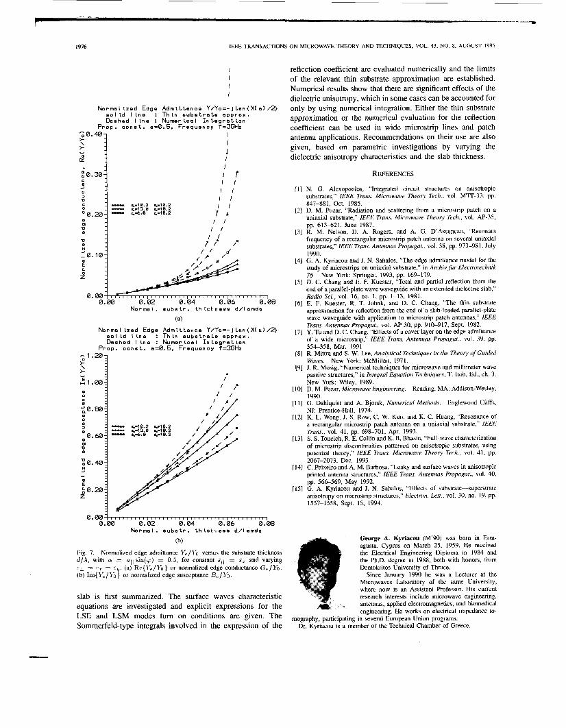
An example showing the dependence of the real (conduc- tance G,) and imaginary (susceptance) part of the normalized edge admittance Y,/Y, from the normalized substrate thick- ness d /X , appears in Fig. 7(a) and (b), respectively. The absolute values of G, and B, can be deduced from these curves by recalling the expression of Yo = nl l / (p&d) . For these curves we have ,uT =1, E ~ I =10.2, f = 3 GHz and G, = 0.0847 . Re(Y,/Yo)/(d/X). Similarly for Be we use the Im(Y,/Yo) instead of the Re part. The effects of the dielectric anisotropy on the edge admittance are quite similar to the above described for the phase and the magnitude of the reflection coefficient.

The above observations and conclusions could be used as a guide in applying this reflection coefficient in the analysis of microstrip lines and patch antennas printed on uniaxial substrate.

The phase of the reflection coefficient R e X ( a ) is involved in the estimation of the propagation constants or the resonant frequencies by establishing transverse resonance conditions. This task requires the solution of transcendental characteristic equations, which in tum involves the reflection coefficient and in some cases more than once with different arguments (Le. triangular patch antennas). Since the th. subs. approximation behaves quite well for the Rex("), even at its worst case with thick substrate and large E L it can be used without any serious doubts within the solution of such equations. In the case when better accuracy is required or when d /X and E L are large, the th. subs. approximation must be used first to get a solution quite close to the actual one. Afterwards a solution scheme employing numerical integration for X ( a ) should be used to improve the accuracy of the solution. In this manner time consuming calculations which require the iterative use of numerical integration are kept at a minimum.

The magnitude of the reflection coefficient is involved in the calculations of the normalized edge admittance, the normalized radiated power (1 - lrl2) and the input impedance of patch antennas. Since these quantities are usually calculated only once at each frequency (or for a specified set of input data) and significant deviations in II'l values between th. subs. approximation and num. integration are observed, the use of the numerical integration in the case of thick substrates is strongly recommended. In the case of electrically thin substrates ( d / X 5 0.02) the th. subs. approximation can be safely used with an error less than 8%.

E I ~ = 2.4).

VIII. CONCLUSION

A Wiener-Hopf-type solution of the canonical problem of a TEM wave falling upon the edge of the truncated upper conductor of a grounded uniaxial anisotropic dielectric

t ”..

L I

2 0.40-

B

* + v

0.30- c a

0 J

J -0

0 c I 00.20: m

m

0 -0

1

1976 IEEE TRANSACTIONS ON MICROWAVE THEORY AND TECHNIQUES, VOL. 43, NO. 8, AUGUST 1995

I I

I I

1

I t I f

I I I !

I / c.-10.2 c.’10.2 - q-13.0 c.=10.2 - 4.6.0 4-10.2 f L I f

I f I ,

;0.10/,,/,> +/< 2’ , , , , I ,

E

0.00 0.00 0.02 0.04 0.06 0.08

N o r m a l . e u b s t r . t h l c t n e s s d / l amda

(a)

N o r m a l l z e d E d g e A d m l t t a n c e Y/Yo=-J t a n { X ( a ) / 2 } s o l I d I l n e : T h l n s u b s t r a t e o p p r o x . D a s h e d I l n e : N u m e r l c o l I n t e g r o t l o n

P r o p . c o n s t . a=0.5. F r e a u e n c v f=3GHz

m 0 c a J ,0.801 m

m

m

0

J

0.601 0 0 m

m 0.401 -0

N d - ; ,L0.20: z

f f #*

4-10.2 4-10.2 - 4-6.8 4-10.2 -c11 4-13.8 q-10.2

0.001 3 I I I I I I I , I I I r I I I I I 8 I I I I I I 8 1 I I I I I I I v I I I I 1 0.00 0.02 0.04 0.06 0.08

Norma I . s u b s t r . t h l c t i , e s s d / l amda

(b)

Fig. 7. Normalized edge admittance Y,/Yo versus the substrate thickness d / A , with cy = nil s in(p) = 0.5, for constant € 1 1 = cr and varying cl = E~ = E ~ . (a) Re{Ye/Yo} or normalized edge conductance G,/Yo. (b) Im{ Ye /YO } or normalized edge susceptance Be /Yo.

slab is first summarized. The surface waves characteristic equations are investigated and explicit expressions for the LSE and LSM modes turn on conditions are given. The Sommerfeld-type integrals involved in the expression of the

reflection coefficient are evaluated numerically and the limits of the relevant thin substrate approximation are established. Numerical results show that there are significant effects of the dielectric anisotropy, which in some cases can be accounted for only by using numerical integration. Either the thin substrate approximation or the numerical evaluation for the reflection coefficient can be used in wide microstrip lines and patch antenna applications. Recommendations on their use are also given, based on parametric investigations by varying the dielectric anisotropy characteristics and the slab thickness.

REFERENCES

N. G. Alexopoulos, “Integrated circuit structures on anisotropic substrates,” IEEE Trans. Microwave Theory Tech., vol. MTI-33, pp. 847-881, Oct. 1985. D. M. Pozar, “Radiation and scattering from a microstrip patch on a uniaxial substrate,” IEEE Trans. Microwave Theory Tech., vol. AP-35, pp. 613-621, June 1987. R. M. Nelson, D. A. Rogers, and A. G. D’Assuncao, “Resonant frequency of a rectangular microstrip patch antenna on several uniaxial substrates,” IEEE Trans. Antennas Propagat., vol. 38, pp. 973-981, July 1990. G. A. Kyriacou and J. N. Sahalos, “The edge admittance model for the study of microstrips on uniaxial substrate,” in Archiv fur Electrotechnik 76. D. C. Chang and E. F. Kuester, “Total and partial reflection from the end of a parallel-plate wave waveguide with an extended dielectric slab,” Radio Sci., vol. 16, no. 1, pp. 1-13, 1981. E. F. Kuester, R. T. Johnk, and D. C. Chang, “The thin substrate approximation for reflection from the end of a slab-loaded parallel-plate wave waveguide with application to microstrip patch antennas,” IEEE Trans. Antennas Propagat., vol. AP-30, pp. 91&917, Sept. 1982. Y. Tu and D. C. Chang, “Effects of a cover layer on the edge admittance of a wide microstrip,” IEEE Trans. Antennas Propagat., vol. 39, pp. 354-358, Mar. 1991. R. Mittra and S. W. Lee, Analytical Techniques in the Theory of Guided Waves. New York: McMillan, 1971. J. R. Mosig, “Numerical techniques for microwave and millimeter wave passive structures,” in Integral Equation Techniques, T. Itoh, Ed., ch. 3. New York: Wiley, 1989. D. M. Pozar, Microwave Engineering. Reading, MA: Addison-Wesley, 1990. G. Dahlquist and A. Bjorsk, Numerical Methods. Englewood Cliffs, NJ: Prentice-Hall, 1974. K. L. Wong, J. S. Row, C. W. Kuo, and K. C. Huang, “Resonance of a rectangular microstrip patch antenna on a uniaxial substrate,” IEEE Trans., vol. 41, pp. 698-701, Apr. 1993. S. S. Toncich, R. E. Collin and K. B. Bhasin, “Full-wave characterization of microstrip discontinuities pattemed on anisotropic substrates, using Dotential theory,” IEEE Trans. Microwave Theory Tech., vol. 41, pp.

New York: Springer, 1993, pp. 169-179.

5067-2073, Dec. 1993. C. Peixeiro and A. M. Barbosa, “Leaky and surface waves in anisotropic printed antenna structures,” IEEE Trans. Antennas Propagat., vol. 40, pp. 566-569, May 1992. G. A. Kyriacou and J. N. Sahalos, “Effects of substrate-superstrate anisotropy on microstrip structures,” Electron. Lett., vol. 30, no. 19, pp. 1557-1558, Sept. 15, 1994.

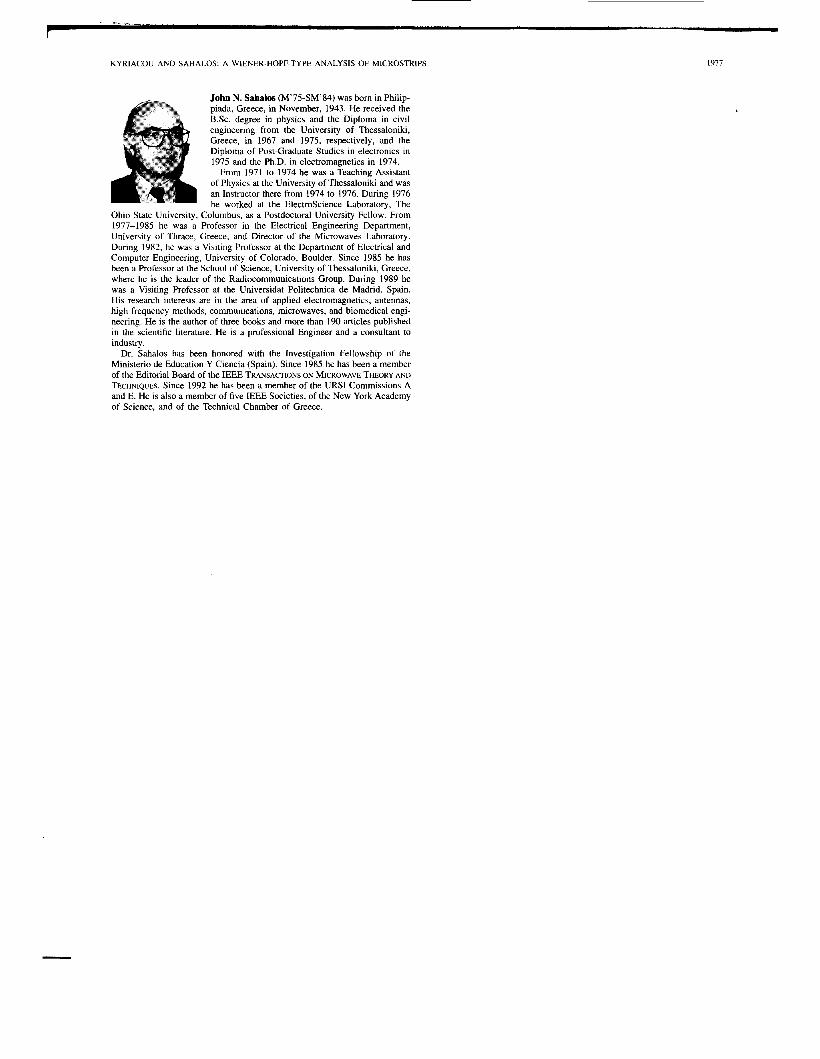
George A. Kyriacou (M’90) was bom in Fam- agusta, Cyprus on March 25, 1959 He received the Electrical Engineenng Diploma in 1984 and the P h D degree in 1988, both wlth honors, from Demokntos University of Thrace

Since January 1990 he was a Lecturer at the Microwaves Laboratory of the same University, where now is an Assistant Professor His current research interests include rmcrowave engineenng, antennas, applied electromagnetics, and biomedical engineenng He works on electncal impedance to-

mography, participating in several European Union programs Dr. Kyriacou IS a member of the Technical Chamber of Greece

KYRIACOU AND SAHALOS: A WIENER-HOPF-TYPE ANALYSIS OF MICROSTRIPS 1977

John N. Sahalos (M’75-SM’84) was born in Philip- piada, Greece, in November, 1943. He received the BSc. degree in physics and the Diploma in civil engineering from the University of Thessaloniki, Greece, in 1967 and 1975, respectively, and the Diploma of Post-Graduate Studies in electronics in 1975 and the Ph.D. in electromagnetics in 1974.

From 1971 to 1974 he was a Teaching Assistant of Physics at the University of Thessaloniki and was an Instructor there from 1974 to 1976 During 1976 he worked at the ElectroScience Laboratory, The

Ohio State University, Columbus, as a Postdoctoral University Fellow. From 1977-1985 he was a Professor in the Electrical Engineering Department, University of Thrace, Greece, and Director of the Microwaves Laboratory. During 1982, he was a Visiting Professor at the Department of Electrical and Computer Engineering, University of Colorado, Boulder. Since 1985 he has been a Professor at the School of Science, University of Thessaloniki, Greece, where he is the leader of the Radiocommunications Group. During 1989 he was a Visiting Professor at the Universidat Politechnica de Madrid, Spain. His research interests are in the area of applied electromagnetics, antennas, high frequency methods, communications, microwaves, and biomedical engi- neering. He is the author of three books and more than 190 articles published in the scientific literature He is a professional Engineer and a consultant to industry.

Dr. Sahalos has been honored with the Investigation Fellowship of the Ministerio de Education Y Ciencia (Spain). Since 1985 he has been a member of the Editorial Board of the IEEE TRANSACTIONS ON MICROWAVE THEORY AND TECHNIQUES. Since 1992 he has been a member of the URSI Comrmssions A and E. He is also a member of five IEEE Societies, of the New York Academy of Science. and of the Technical Chamber of Greece.