Embed Size (px)
Citation preview
JOURNAL OF COMPUTATIONAL PHYSICS 132, 3–11 (1997)ARTICLE NO. CP965514
A Well-Behaved TVD Limiter for High-Resolution Calculations ofUnsteady Flow
Mohit Arora and Philip L. Roe
Department of Aerospace Engineering, University of Michigan, Ann Arbor, Michigan 48109-2118
Received October 16, 1995; revised May 13, 1996
For the most part, the analysis was subsequently appliedto finding steady solutions as the large-time limit of aA total variation diminishing (TVD) limiter is proposed that at-
tempts to maximize performance given that the inherent limitation (pseudo) unsteady flow. Retaining the dependence on theof TVD formulations is peak loss. For the scalar advection and Burg- Courant number shows little advantage in these circum-er’s equation, the present results are qualitatively superior to those stances, and the simplified conditionusing the harmonic and superbee limiters, balancing well the com-peting effects of skewing, smearing, and squaring. In the case of the
F(r) # min(2, 2r)Euler equations, the current results appear to significantly improveupon previous TVD results and are quite comparable with moreelaborate algorithms. Q 1997 Academic Press is more economical. Additionally, if the limiter has the
symmetry property
1. INTRODUCTION
F S1rD5
1r
F(r),Control of oscillations in high-resolution schemes con-
tinues to be a topic of interest and importance. Manymethods are based on Harten’s concept of a total varia- then simplified reconstruction techniques [23] can be usedtion diminishing (TVD) scheme, which prevents, in the that reduce the computational cost.scalar case, any values being generated after n 1 1 time These simplifications do, however, reduce the effective-steps that lie outside the range of those present after n ness of TVD schemes in their original setting of unsteadytime steps. There are several other properties that are flow, and it is these simplified schemes that have usuallyloosely equivalent—positivity [21], the characteristic in- been compared with ENO schemes, much to the advantageterpolation property [15], or local extremum diminishing of the latter. The object of the present paper is to point[7]. If any of these conditions apply, then the amplitude out that TVD schemes, as originally conceived, are not inof any genuine extremum can only decrease, and there fact inferior to the simpler kinds of ENO schemes and canis a progressive loss of information concerning high- be substantially cheaper. We do not wish to over-sell thefrequency waves. product and readily concede that elaborate ENO schemes
To remedy this, Harten et al. [4, 5] introduced the idea can give superior performance. We do, however, wish toof essentially nonoscillatory (ENO) schemes, which allow correct the impression that TVD schemes are without meritthe loss of amplitude at one step to be regained at another. for unsteady flow.Numerous comparison studies show that ENO schemes The cost of the proposed limiter is one call each to thepreserve the high-frequency information better than TVD max and min functions, the same as for the minmod limiter.schemes. Usually, however, the comparison is made with This limiter is now new [12, 16] and has recently beenan inferior TVD method. suggested by Jeng and Payne [8] as a basis for an adaptive
This seems to have an historical origin. Early studies of limiter with shock-detection features. Neither is it perfect;flux-limiter schemes [13, 16, 17, 22] were based on unsteady there is a limit (pun intended) to what can be accomplishedanalysis of the advection equation and retained the with the fixed stencil of a TVD scheme. Having said that,Courant number n 5 a Dt/Dx as a parameter in the analysis, it does perform much better than the TVD schemes pres-leading to constraints (the notation is defined later) ently in common use.
2. DESIGNING THE LIMITER
F(r) # min S 21 2 n
,2rn D .
Ideally, a limiter should possess the following properties:
30021-9991/97 $25.00
Copyright 1997 by Academic PressAll rights of reproduction in any form reserved.
4 ARORA AND ROE
1. be a homogeneous function to be the slope corresponding to the third order schemeat the point (1, 1) in (r, F) coordinates, viz.,2. satisfy the TVD constraints
3. be as accurate as possible in smooth regions
4. revert to the underlying first-order scheme at ex- s2 5 S1 1 n3 D , (2.1)
trema and discontinuities
5. be computationally simple and economicalwhich fully determines the proposed limiter function. This6. convert smooth profiles without undue distortionlimiter function was used by Roe and Baines [12, 16] almost
7. convect discontinuities without much smearing 15 years ago. More recently, this function was utilized by8. accomplish all of the above for a wide range of Jeng and Payne [8] in the context of an adaptive limiter;
Courant numbers. because of the stress placed on discontinuity capturing in[8], the authors perhaps undervalued it as a general-pur-To be successful at all Courant numbers, it is highlypose limiter. Although TVD schemes in general cannot beprobable that some dependence on this parameter mustbetter than second-order accurate, this particular limiterbe retained. The behavior of the superbee limiter near thebestows some properties characteristic of third-orderpoint (1, 1) is designed [13] to bestow a discontinuity-schemes. Experiments reported in [12] demonstrated thatcapturing property for linear waves. It has proved difficultfor linear advection the width of a discontinuity in theto retain this without also having to accept a tendencyinitial data spreads like t1/4, rather than the t1/3 typicalto ‘‘square off’’ smooth profiles, but if this is tolerable,of second-order methods. This is reflected in the excellentsuperbee remains a good choice. An alternative criterionresolution of contact discontinuities in the results below.for the behavior near (1, 1), also noted in [13], is to choose
Note that the stability restriction on the method is simplythe unique slope at that point that gives third-order accu-unu # 1.0.racy in the one-dimensional constant coefficient case. This
For non-linear systems, the full TVD region has beenleads to a class of limiters given byempirically found to be too compressive and hence we usethe more restrictive TVD constraints of s1 5 Fmax 5 2 for
F(s1 , s2 , Fmax , r) 5 max[0, minhs1r, 1 1 s2(r 2 1), Fmaxj]. the nonlinear waves while using the full TVD region forthe linear waves. This bound could probably be relaxedfor problems involving only weak shocks. This is analogousThis function is made up of three straight-line segments,
two of which are fully determined by the TVD constraints, to the popular implementation of using the harmonic lim-iter on the non-linear waves and the Superbee limiter oni.e., s1 5 2/n and Fmax 5 2/(1 2 n). The segment that
remains to be determined is the middle one. Observe that the linear waves. Researchers who follow this practicemight find that the present limiter would also be an appro-it must pass through the point (1, 1) in order to revert to
the second-order scheme in smooth regions. We choose s2 priate choice for the linear fields.
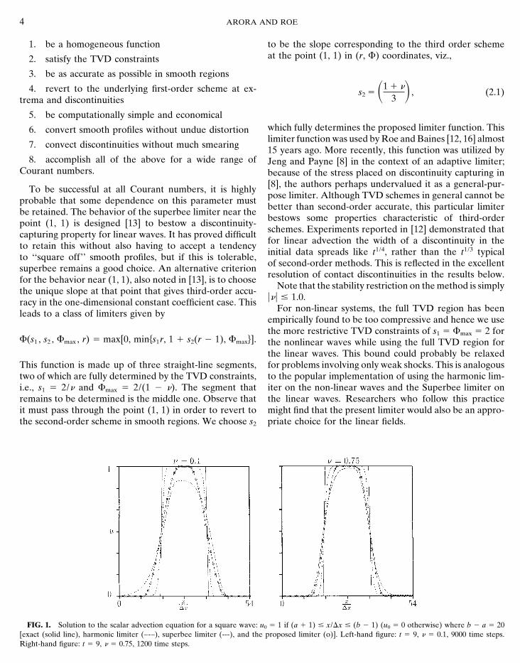
FIG. 1. Solution to the scalar advection equation for a square wave: u0 5 1 if (a 1 1) # x/Dx # (b 2 1) (u0 5 0 otherwise) where b 2 a 5 20[exact (solid line), harmonic limiter (–-–), superbee limiter (---), and the proposed limiter (o)]. Left-hand figure: t 5 9, n 5 0.1, 9000 time steps.Right-hand figure: t 5 9, n 5 0.75, 1200 time steps.
HIGH-RESOLUTION UNSTEADY FLOW CALCULATIONS 5
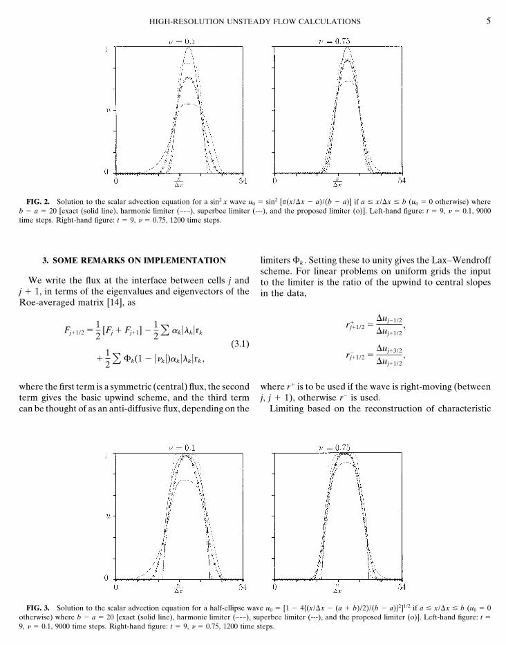
FIG. 2. Solution to the scalar advection equation for a sin2 x wave u0 5 sin2 [f(x/Dx 2 a)/(b 2 a)] if a # x/Dx # b (u0 5 0 otherwise) whereb 2 a 5 20 [exact (solid line), harmonic limiter (–-–), superbee limiter (---), and the proposed limiter (o)]. Left-hand figure: t 5 9, n 5 0.1, 9000time steps. Right-hand figure: t 5 9, n 5 0.75, 1200 time steps.
3. SOME REMARKS ON IMPLEMENTATION limiters Fk . Setting these to unity gives the Lax–Wendroffscheme. For linear problems on uniform grids the input
We write the flux at the interface between cells j and to the limiter is the ratio of the upwind to central slopesj 1 1, in terms of the eigenvalues and eigenvectors of the in the data,Roe-averaged matrix [14], as
r1j11/2 5
Duj21/2
Duj11/2,
Fj11/2 512
[Fj 1 Fj11] 212 O akulkurk
(3.1)r2
j11/2 5Duj13/2
Duj11/2,1
12 O Fk(1 2 unku)akulkurk ,
where the first term is a symmetric (central) flux, the second where r1 is to be used if the wave is right-moving (betweenj, j 1 1), otherwise r2 is used.term gives the basic upwind scheme, and the third term
can be thought of as an anti-diffusive flux, depending on the Limiting based on the reconstruction of characteristic
FIG. 3. Solution to the scalar advection equation for a half-ellipse wave u0 5 [1 2 4h(x/Dx 2 (a 1 b)/2)/(b 2 a)j2]1/2 if a # x/Dx # b (u0 5 0otherwise) where b 2 a 5 20 [exact (solid line), harmonic limiter (–-–), superbee limiter (---), and the proposed limiter (o)]. Left-hand figure: t 5
9, n 5 0.1, 9000 time steps. Right-hand figure: t 5 9, n 5 0.75, 1200 time steps.
6 ARORA AND ROE
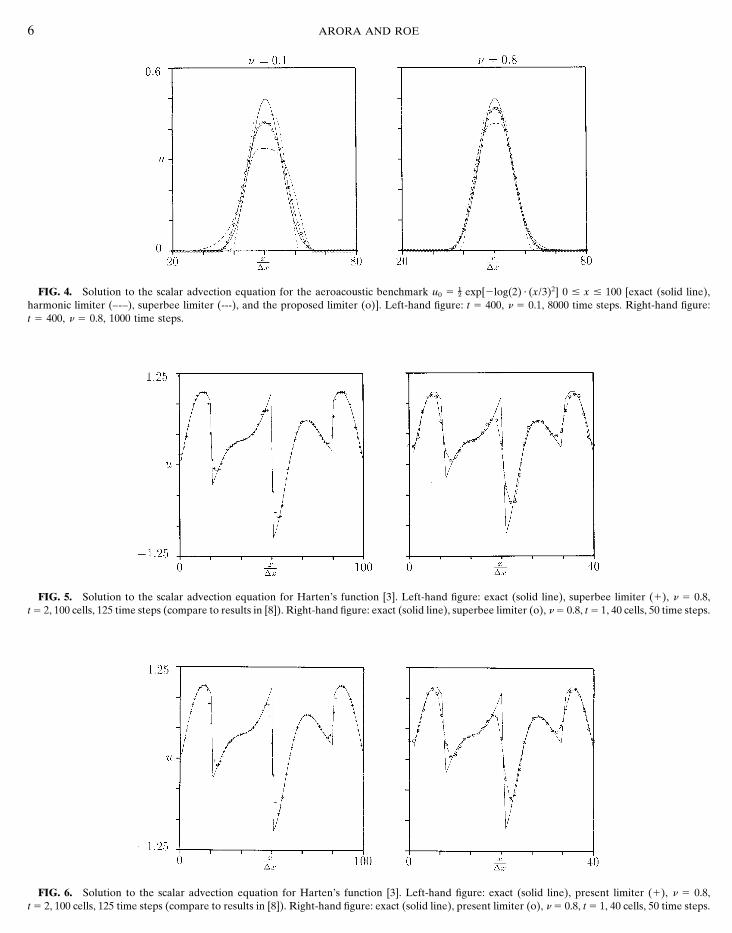
FIG. 4. Solution to the scalar advection equation for the aeroacoustic benchmark u0 5 As exp[2log(2) ? (x/3)2] 0 # x # 100 [exact (solid line),harmonic limiter (–-–), superbee limiter (---), and the proposed limiter (o)]. Left-hand figure: t 5 400, n 5 0.1, 8000 time steps. Right-hand figure:t 5 400, n 5 0.8, 1000 time steps.
FIG. 5. Solution to the scalar advection equation for Harten’s function [3]. Left-hand figure: exact (solid line), superbee limiter (1), n 5 0.8,t 5 2, 100 cells, 125 time steps (compare to results in [8]). Right-hand figure: exact (solid line), superbee limiter (o), n 5 0.8, t 5 1, 40 cells, 50 time steps.
FIG. 6. Solution to the scalar advection equation for Harten’s function [3]. Left-hand figure: exact (solid line), present limiter (1), n 5 0.8,t 5 2, 100 cells, 125 time steps (compare to results in [8]). Right-hand figure: exact (solid line), present limiter (o), n 5 0.8, t 5 1, 40 cells, 50 time steps.
HIGH-RESOLUTION UNSTEADY FLOW CALCULATIONS 7
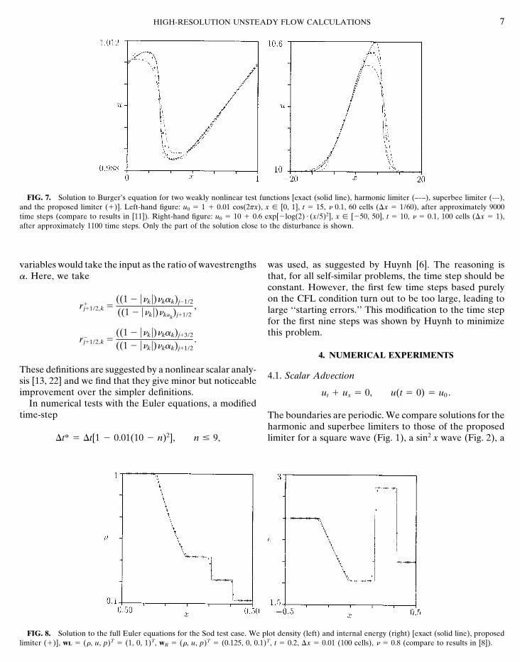
FIG. 7. Solution to Burger’s equation for two weakly nonlinear test functions [exact (solid line), harmonic limiter (–-–), superbee limiter (---),and the proposed limiter (1)]. Left-hand figure: u0 5 1 1 0.01 cos(2fx), x [ [0, 1], t 5 15, n 0.1, 60 cells (Dx 5 1/60), after approximately 9000time steps (compare to results in [11]). Right-hand figure: u0 5 10 1 0.6 exp[2log(2) ? (x/5)2], x [ [250, 50], t 5 10, n 5 0.1, 100 cells (Dx 5 1),after approximately 1100 time steps. Only the part of the solution close to the disturbance is shown.
variables would take the input as the ratio of wavestrengths was used, as suggested by Huynh [6]. The reasoning isthat, for all self-similar problems, the time step should bea. Here, we takeconstant. However, the first few time steps based purelyon the CFL condition turn out to be too large, leading to
r1j11/2,k 5
((1 2 unku)nkak)j21/2
((1 2 unku)nkak)j11/2
, large ‘‘starting errors.’’ This modification to the time stepfor the first nine steps was shown by Huynh to minimizethis problem.
r2j11/2,k 5
((1 2 unku)nkak)j13/2
((1 2 unku)nkak)j11/2.
4. NUMERICAL EXPERIMENTS
These definitions are suggested by a nonlinear scalar analy-4.1. Scalar Advectionsis [13, 22] and we find that they give minor but noticeable
improvement over the simpler definitions. ut 1 ux 5 0, u(t 5 0) 5 u0 .In numerical tests with the Euler equations, a modified
time-step The boundaries are periodic. We compare solutions for theharmonic and superbee limiters to those of the proposedlimiter for a square wave (Fig. 1), a sin2 x wave (Fig. 2), aDt* 5 Dt[1 2 0.01(10 2 n)2], n # 9,
FIG. 8. Solution to the full Euler equations for the Sod test case. We plot density (left) and internal energy (right) [exact (solid line), proposedlimiter (1)], wL 5 (r, u, p)T 5 (1, 0, 1)T, wR 5 (r, u, p)T 5 (0.125, 0, 0.1)T, t 5 0.2, Dx 5 0.01 (100 cells), n 5 0.8 (compare to results in [8]).
8 ARORA AND ROE
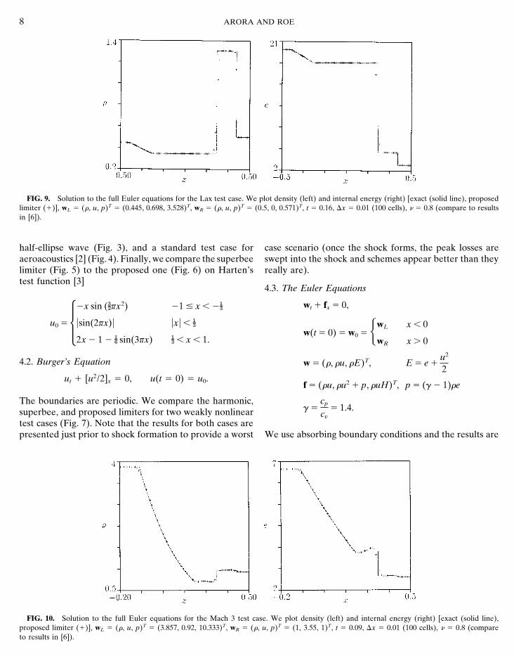
FIG. 9. Solution to the full Euler equations for the Lax test case. We plot density (left) and internal energy (right) [exact (solid line), proposedlimiter (1)], wL 5 (r, u, p)T 5 (0.445, 0.698, 3.528)T, wR 5 (r, u, p)T 5 (0.5, 0, 0.571)T, t 5 0.16, Dx 5 0.01 (100 cells), n 5 0.8 (compare to resultsin [6]).
half-ellipse wave (Fig. 3), and a standard test case for case scenario (once the shock forms, the peak losses areswept into the shock and schemes appear better than theyaeroacoustics [2] (Fig. 4). Finally, we compare the superbee
limiter (Fig. 5) to the proposed one (Fig. 6) on Harten’s really are).test function [3]
4.3. The Euler Equations
wt 1 fx 5 0,
u0 5 52x sin (Dsfx2) 21 # x , 2Ad
usin(2fx)u uxu , Ad
2x 2 1 2 Ah sin(3fx) Ad , x , 1.w(t 5 0) 5 w0 5HwL x , 0
wR x . 0
4.2. Burger’s Equation w 5 (r, ru, rE)T, E 5 e 1u2
2ut 1 [u2/2]x 5 0, u(t 5 0) 5 u0. f 5 (ru, ru2 1 p, ruH)T, p 5 (c 2 1)re
The boundaries are periodic. We compare the harmonic,c 5
cp
cv5 1.4.superbee, and proposed limiters for two weakly nonlinear
test cases (Fig. 7). Note that the results for both cases arepresented just prior to shock formation to provide a worst We use absorbing boundary conditions and the results are
FIG. 10. Solution to the full Euler equations for the Mach 3 test case. We plot density (left) and internal energy (right) [exact (solid line),proposed limiter (1)], wL 5 (r, u, p)T 5 (3.857, 0.92, 10.333)T, wR 5 (r, u, p)T 5 (1, 3.55, 1)T, t 5 0.09, Dx 5 0.01 (100 cells), n 5 0.8 (compareto results in [6]).
HIGH-RESOLUTION UNSTEADY FLOW CALCULATIONS 9
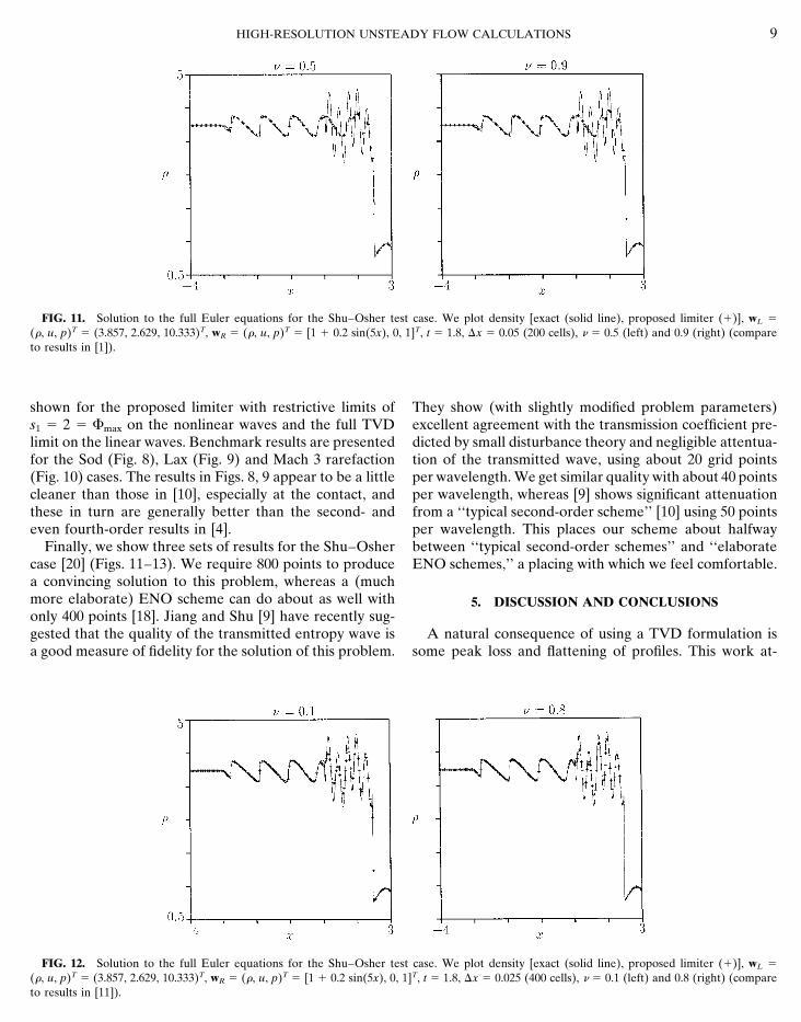
FIG. 11. Solution to the full Euler equations for the Shu–Osher test case. We plot density [exact (solid line), proposed limiter (1)], wL 5
(r, u, p)T 5 (3.857, 2.629, 10.333)T, wR 5 (r, u, p)T 5 [1 1 0.2 sin(5x), 0, 1]T, t 5 1.8, Dx 5 0.05 (200 cells), n 5 0.5 (left) and 0.9 (right) (compareto results in [1]).
shown for the proposed limiter with restrictive limits of They show (with slightly modified problem parameters)excellent agreement with the transmission coefficient pre-s1 5 2 5 Fmax on the nonlinear waves and the full TVD
limit on the linear waves. Benchmark results are presented dicted by small disturbance theory and negligible attentua-tion of the transmitted wave, using about 20 grid pointsfor the Sod (Fig. 8), Lax (Fig. 9) and Mach 3 rarefaction
(Fig. 10) cases. The results in Figs. 8, 9 appear to be a little per wavelength. We get similar quality with about 40 pointsper wavelength, whereas [9] shows significant attenuationcleaner than those in [10], especially at the contact, and
these in turn are generally better than the second- and from a ‘‘typical second-order scheme’’ [10] using 50 pointsper wavelength. This places our scheme about halfwayeven fourth-order results in [4].
Finally, we show three sets of results for the Shu–Osher between ‘‘typical second-order schemes’’ and ‘‘elaborateENO schemes,’’ a placing with which we feel comfortable.case [20] (Figs. 11–13). We require 800 points to produce
a convincing solution to this problem, whereas a (muchmore elaborate) ENO scheme can do about as well with 5. DISCUSSION AND CONCLUSIONSonly 400 points [18]. Jiang and Shu [9] have recently sug-gested that the quality of the transmitted entropy wave is A natural consequence of using a TVD formulation is
some peak loss and flattening of profiles. This work at-a good measure of fidelity for the solution of this problem.
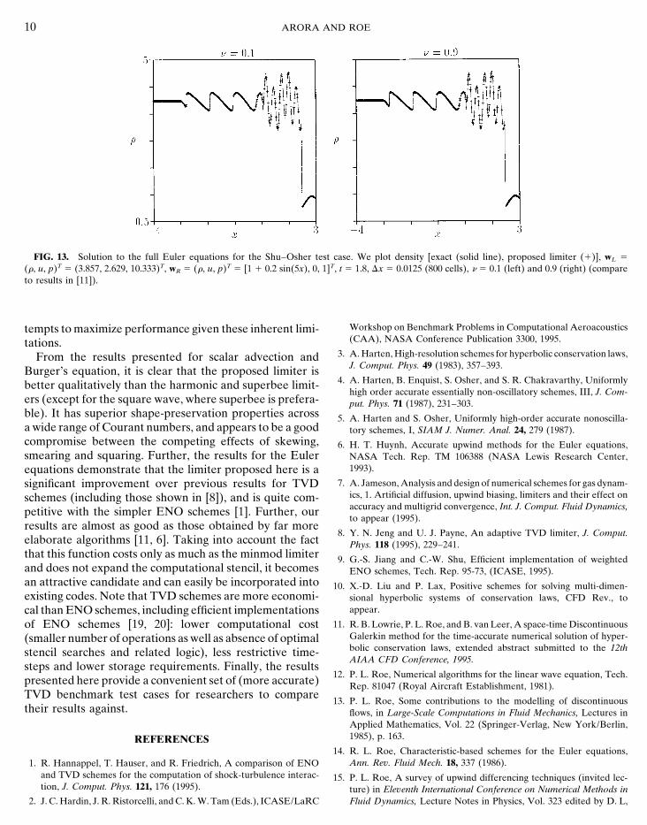
FIG. 12. Solution to the full Euler equations for the Shu–Osher test case. We plot density [exact (solid line), proposed limiter (1)], wL 5
(r, u, p)T 5 (3.857, 2.629, 10.333)T, wR 5 (r, u, p)T 5 [1 1 0.2 sin(5x), 0, 1]T, t 5 1.8, Dx 5 0.025 (400 cells), n 5 0.1 (left) and 0.8 (right) (compareto results in [11]).
10 ARORA AND ROE
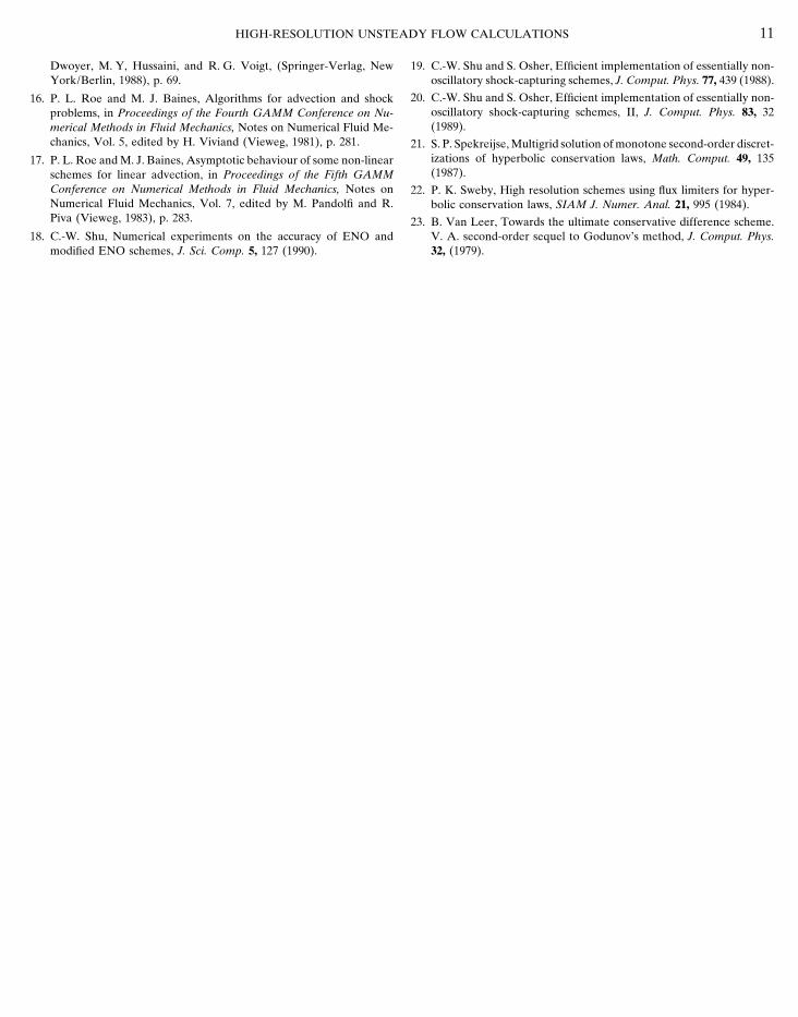
FIG. 13. Solution to the full Euler equations for the Shu–Osher test case. We plot density [exact (solid line), proposed limiter (1)], wL 5
(r, u, p)T 5 (3.857, 2.629, 10.333)T, wR 5 (r, u, p)T 5 [1 1 0.2 sin(5x), 0, 1]T, t 5 1.8, Dx 5 0.0125 (800 cells), n 5 0.1 (left) and 0.9 (right) (compareto results in [11]).
Workshop on Benchmark Problems in Computational Aeroacousticstempts to maximize performance given these inherent limi-(CAA), NASA Conference Publication 3300, 1995.tations.
3. A. Harten, High-resolution schemes for hyperbolic conservation laws,From the results presented for scalar advection andJ. Comput. Phys. 49 (1983), 357–393.Burger’s equation, it is clear that the proposed limiter is
4. A. Harten, B. Enquist, S. Osher, and S. R. Chakravarthy, Uniformlybetter qualitatively than the harmonic and superbee limit-high order accurate essentially non-oscillatory schemes, III, J. Com-
ers (except for the square wave, where superbee is prefera- put. Phys. 71 (1987), 231–303.ble). It has superior shape-preservation properties across 5. A. Harten and S. Osher, Uniformly high-order accurate nonoscilla-a wide range of Courant numbers, and appears to be a good tory schemes, I, SIAM J. Numer. Anal. 24, 279 (1987).compromise between the competing effects of skewing, 6. H. T. Huynh, Accurate upwind methods for the Euler equations,smearing and squaring. Further, the results for the Euler NASA Tech. Rep. TM 106388 (NASA Lewis Research Center,
1993).equations demonstrate that the limiter proposed here is a7. A. Jameson, Analysis and design of numerical schemes for gas dynam-significant improvement over previous results for TVD
ics, 1. Artificial diffusion, upwind biasing, limiters and their effect onschemes (including those shown in [8]), and is quite com-accuracy and multigrid convergence, Int. J. Comput. Fluid Dynamics,petitive with the simpler ENO schemes [1]. Further, ourto appear (1995).
results are almost as good as those obtained by far more8. Y. N. Jeng and U. J. Payne, An adaptive TVD limiter, J. Comput.
elaborate algorithms [11, 6]. Taking into account the fact Phys. 118 (1995), 229–241.that this function costs only as much as the minmod limiter 9. G.-S. Jiang and C.-W. Shu, Efficient implementation of weightedand does not expand the computational stencil, it becomes ENO schemes, Tech. Rep. 95-73, (ICASE, 1995).an attractive candidate and can easily be incorporated into 10. X.-D. Liu and P. Lax, Positive schemes for solving multi-dimen-existing codes. Note that TVD schemes are more economi- sional hyperbolic systems of conservation laws, CFD Rev., to
appear.cal than ENO schemes, including efficient implementations11. R. B. Lowrie, P. L. Roe, and B. van Leer, A space-time Discontinuousof ENO schemes [19, 20]: lower computational cost
Galerkin method for the time-accurate numerical solution of hyper-(smaller number of operations as well as absence of optimalbolic conservation laws, extended abstract submitted to the 12thstencil searches and related logic), less restrictive time-AIAA CFD Conference, 1995.
steps and lower storage requirements. Finally, the results12. P. L. Roe, Numerical algorithms for the linear wave equation, Tech.presented here provide a convenient set of (more accurate) Rep. 81047 (Royal Aircraft Establishment, 1981).
TVD benchmark test cases for researchers to compare13. P. L. Roe, Some contributions to the modelling of discontinuous
their results against. flows, in Large-Scale Computations in Fluid Mechanics, Lectures inApplied Mathematics, Vol. 22 (Springer-Verlag, New York/Berlin,1985), p. 163.REFERENCES
14. R. L. Roe, Characteristic-based schemes for the Euler equations,Ann. Rev. Fluid Mech. 18, 337 (1986).1. R. Hannappel, T. Hauser, and R. Friedrich, A comparison of ENO
and TVD schemes for the computation of shock-turbulence interac- 15. P. L. Roe, A survey of upwind differencing techniques (invited lec-tion, J. Comput. Phys. 121, 176 (1995). ture) in Eleventh International Conference on Numerical Methods in
Fluid Dynamics, Lecture Notes in Physics, Vol. 323 edited by D. L,2. J. C. Hardin, J. R. Ristorcelli, and C. K. W. Tam (Eds.), ICASE/LaRC
HIGH-RESOLUTION UNSTEADY FLOW CALCULATIONS 11
Dwoyer, M. Y, Hussaini, and R. G. Voigt, (Springer-Verlag, New 19. C.-W. Shu and S. Osher, Efficient implementation of essentially non-oscillatory shock-capturing schemes, J. Comput. Phys. 77, 439 (1988).York/Berlin, 1988), p. 69.
20. C.-W. Shu and S. Osher, Efficient implementation of essentially non-16. P. L. Roe and M. J. Baines, Algorithms for advection and shockoscillatory shock-capturing schemes, II, J. Comput. Phys. 83, 32problems, in Proceedings of the Fourth GAMM Conference on Nu-(1989).merical Methods in Fluid Mechanics, Notes on Numerical Fluid Me-
chanics, Vol. 5, edited by H. Viviand (Vieweg, 1981), p. 281. 21. S. P. Spekreijse, Multigrid solution of monotone second-order discret-izations of hyperbolic conservation laws, Math. Comput. 49, 13517. P. L. Roe and M. J. Baines, Asymptotic behaviour of some non-linear(1987).schemes for linear advection, in Proceedings of the Fifth GAMM
Conference on Numerical Methods in Fluid Mechanics, Notes on 22. P. K. Sweby, High resolution schemes using flux limiters for hyper-Numerical Fluid Mechanics, Vol. 7, edited by M. Pandolfi and R. bolic conservation laws, SIAM J. Numer. Anal. 21, 995 (1984).Piva (Vieweg, 1983), p. 283. 23. B. Van Leer, Towards the ultimate conservative difference scheme.
V. A. second-order sequel to Godunov’s method, J. Comput. Phys.18. C.-W. Shu, Numerical experiments on the accuracy of ENO andmodified ENO schemes, J. Sci. Comp. 5, 127 (1990). 32, (1979).