Embed Size (px)
Citation preview
A Welch-Satterthwaite Relation for Correlated Errors1
Dr. Howard Castrup Integrated Sciences Group 14608 Casitas Canyon Rd.
Bakersfield, CA 93306 661-872-1683
[email protected] Abstract
The Welch-Satterthwaite relation provides a useful tool for estimating the degrees of freedom for uncertainty estimates for measurement errors comprised of a linear sum of s-independent normally distributed quantities with different variances. Working from a derivation for the degrees of freedom of Type B uncertainty estimates, a variation of the Welch-Satterthwaite relation is developed that is applicable to combinations of errors that are both s-independent and correlated. Expressions for each case are provided for errors arising from both direct and multivariate measurements. 1. Introduction
1.1 Background
The Welch-Satterthwaite relation provides a means of computing the degrees of freedom for an uncertainty estimate uT of an error T composed of a linear combination of s-independent errors. If T is comprised of n errors, with respective uncertainties ui, i = 1, 2,…, n, the Welch-Satterthwaite relation can be found in the GUM [1] and elsewhere. It is expressed as
4
4
1
Tn
i
ii
u
u
, (1)
where i is the degrees of freedom for the ith estimate ui. The derivation of this expression is given later in Section 3.1. Since a central purpose of this paper is to provide a variation of Eq. (1) that applies to correlated as well as uncorrelated errors, we stress the point that that Eq. (1) is strictly applicable only to the former. The development of a more generalized form has been attempted in previous work [2, 3]. In this paper we employ a direct error modeling approach, often applied to building error models for multivariate measurements [1, 4, 5, 6].2 This involves obtaining statistical variances of errors in uncertainty estimates which are used to generalize Eq. (1) to correlated errors. The error modeling approach is given in Section 2.3.1.
1.2 Note to Readers
The use of statistical language and operators in the derivations in this paper suggests that it be read in detail only by those familiar with such technical matter. However, readers interested in just the results of the work will find the essential analytical relations presented in Eq. (9), Eqs. (41) - (43) and in Section 3.3.3. For readers without formal statistical training who wish to follow the derivations, the essential concepts are those of s-independence, expectation value, correlation and covariance, along with some familiarity with the chi-square and normal distributions. The necessary background information can be found in beginning texts on mathematical statistics.
1 Revised March 27, 2010 and May 8, 2020 from Castrup, H., “A Welch-Satterthwaite Relation for Correlated Errors,” Proc. 2010 Meas. Sci. Conf., Pasadena, March 26, 2010. 2 Chapter 6 of Ref. [6] provides a particularly clear and comprehensive discussion of this topic.
- 1 -
2. Degrees of Freedom
The amount of information used to estimate the uncertainty in a given measurement error is quantified by the degrees of freedom. The degrees of freedom is required, among other things, to employ an uncertainty estimate in computing confidence limits and in conducting statistical tests. 2.1 Type A Degrees of Freedom
A Type A uncertainty estimate is a standard deviation computed from a sample of data. Often, the sample standard deviation represents the uncertainty due to random error or repeatability accompanying a measurement. The degrees of freedom for this uncertainty is given by
1n , (2)
where n is the sample size. 2.2 Type B Degrees of Freedom
A Type B estimate is, by definition, an estimate obtained without recourse to a sample of data. Accordingly, for a Type B estimate, a sample size is not directly available but can be estimated. 2.3 Estimating the Degrees of Freedom for a Type B Uncertainty Estimate
In the late 1980s and early 1990s it was recognized that a Type B estimate could not be rigorously applied in computing confidence intervals or in statistical hypothesis testing. The principal reason for this is because, although a Type B estimate of a population standard deviation could be computed, the accompanying degrees of freedom was not readily forthcoming. Without the degrees of freedom, appropriate confidence multipliers, such as t-statistics, commensurate with specified confidence levels, could not be applied, and confidence limits could not be developed. This led to the introduction of such things as “coverage factors” and “expanded uncertainties” to serve as loose substitutes for confidence multipliers and confidence limits. As has been pointed out [7], the use of non-statistical coverage factors to obtain expanded uncertainties is not equivalent to applying t-statistics to obtain confidence limits. In the author's experience, using nominal (often arbitrary) coverage factors and applying the term "expanded uncertainty" have led to incorrect inferences and expensive miscommunications. Clearly, what is needed is a method for obtaining Type B uncertainty estimates and degrees of freedom in such a way that we can return to the development of confidence limits and restore statistical meaning to uncertainty estimates. Such a method is outlined in the next section. 2.3.1 The Derivation
In measurement uncertainty analysis, the uncertainty u in the value of an error x is given by the standard deviation of the error’s probability distribution. To be consistent with articles written of the subject of Type B degrees of freedom [7, 10], we use the notation u = (x). Accordingly, 2(x) represents the distribution variance
2 ( ) var( ) ( )2x x E x , (3)
where the function E(.) represents the statistical expectation value.3 Let s represent the standard deviation computed for a sample of size n of a N(0, 2
) variable x. Since x is N(0, 2 ),
a variable y = 2 /s2 is 2-distributed with = n – 1 degrees of freedom. The pdf is given by
( 2)/2 /2
/2( )
22
xy ef y
. (4)
2 2 2( ) var( ) ( ) ( )
3 The complete expression is
x x E x E x .
However, for measurement errors, the expectation value E(x) is ordinarily assumed to be zero and Eq. (3) is applicable.
- 2 -
Accordingly, since
y = 2 2/s ,
then
2 2 /s y ,
and
4
22
var vars y
. (5)
Note that, for a 2-distributed variable y, var 2y , (6)
so that
4
2 2var s
, (7)
and
4
22
var( )s
. (8)
We now generalize Eq. (8) to any standard deviation estimate u with nonzero var(u2) and write
4
22
var( )u
.
Finally, we estimate the population standard deviation with the uncertainty estimate u and write
4
2 22
( )
u
u
, (9)
where the shorthand notation 2(u2) = var(u2) is used as before. Clearly, the key to applying Eq. (9) is obtaining an estimate of (u2). The lack of a rigorous method for doing this has been the obstacle in determining the degrees of freedom for Type B estimates that has led to the aforementioned use of arbitrary multipliers and the virtual abandonment of confidence limits in favor or expanded uncertainties. To obtain the variance 2(u2) for a Type B estimate u, we employ a simple relation between error containment limits ±L and a containment probability p
( )
Lu
p . (10)
For N(0, 2) errors, the function (p) is given by
1 1( )
2
pp
, (11)
where is the normal distribution function.
Let L and p represent errors in L and p, respectively. Then the error in u2 can be obtained in terms of the errors in L and p using the first-order Taylor series expansion
2 2
2( ) L p
u uu
L p
. (12)
Note that the variance in u2 is synonymous with the variance in (u2). Hence, in keeping with Eq. (3),
- 3 -
2 2 2 2 2 2
2 22 22 2
2 22 2
2 22 22 2
( ) var( ) var[ ( )] [ ( )]
( ) ( )
var( ) var( )
,
L p
L p
L p
u u u E u
u uE E
L p
u u
L p
u uu u
L p
(13)
whereL and p are assumed to be s-independent, and where uL is the uncertainty in the containment limit L and up is the uncertainty in the containment probability p. In Eq. (13), the relations
2 2 2var( ) ( )LL L Lu u E
and 2 2 2var( ) ( )
pp p pu u E
were used. It now remains to determine the partial derivates. From Eq. (10) we get
2
2
2
( )
u
L p
L (14)
and
2 2
3
2
( )
u L
p p
d
dp
. (15)
The derivative d /dp is obtained easily. We first establish that
2( )
/21 1( )
2 2
pp
p e
.
Then, taking the derivative of both sides of this expression yields
2 ( ) / 21 1
2 2p d
edp
,
from which we get
2 ( ) / 2
2pd
edp
. (16)
Substituting in Eq. (15) gives
2
2 2( ) / 2
3
2
( ) 2pu L
ep p
. (17)
Combining Eqs. (17) and (14) in Eq. (13), yields
2
242 2 ( ) 2
4 2 2
4 1( )
( ) ( ) 2pL
p
uLu
p L p
e u
, (18)
and substituting Eq. (18) in Eq. (9) and using Eq. (10) yields
2
12( ) 2
2 2
1 1.
2 2( )pL
pu
e uL p
(19)
- 4 -
2.3.2 Comparison with Eq. G3 of the GUM
Eq. G3 of Annex G of the GUM [1] provides an expression for the degrees of freedom for a Type B estimate4
2
2
1
2
u
u
. (20)
From Eq. (10), we have
2
( )
1.
( ) ( )
L p
L p
u uu
L p
L d
p p dp
(21)
Substituting from Eq. (16) gives
2 ( )/22
1( )
( ) ( ) 2p
L p
Lu e
p p
.
Applying the variance operator, we have
2
2
2 2
22
222 2
22 (
2 4
22 (
2 2
( ) var( ) var[ ( )] ( )
var( ) var( )
1
( ) ( ) 2
1.
( ) ( ) 2
) 2
) 2
L p
L p
pL p
pL p
u u u E u
u u
L p
u uu u
L p
Lu e
p p
Lu e
p p
u
u
(22)
Substituting from Eqs. (10) and (22) in Eq. (20) gives
2
12( ) 2
2 2
1 1
2 2( )pL
pu
e uL p
. (23)
Comparison of Eq. (23) with Eq. (19) shows that using either Eq. (9), derived in this paper, or Eq. G3 of the GUM yields the same result. 2.3.3 Estimating uL and up
The process of assembling the recollected experience and other technical data needed for developing Type B degrees of freedom estimates can be facilitated through the use of standardized formats. Rather than forcing us to estimate error standard deviations and degrees of freedom directly, these formats construct such estimates from information that is readily available to experienced metrologists, calibration technicians and calibration engineers. Three formats are have been found useful.5 In all three formats, the uncertainty is computed using Eq. (10). 2.3.3.1 Format 1
In applying Format 1, we obtain the necessary information by employing the statement
4 Eq. G3 of the GUM can be obtained from Eq. (9). The derivation is presented in Appendix A of this paper. 5 These formats are embodied in the software applications UncertaintyAnalyzer [8] and Uncertainty Sidekick Pro [9] and in the Type B Degrees of Freedom Calculator [10] and Uncertainty Sidekick [11] freeware applications.
- 5 -
“Approximately C% of values ( ±c% ) have been observed to lie within ±L ( ±L )”
In Format 1, c and L represent the lack of information available for the parameters p and L. In this usage, the containment limits are expressed as “L give or take L” and the percent containment is expressed as “C% give or take c%.”6 The estimated containment probability p is given by
p = C / 100,
and a variable p is obtained from p = c / 100.
And, as before, we have
1( ) (1 ) / 2p p .
If error limits L and p can be estimated for L and p, respectively, then the uncertainties uL and up can be estimated using the uniform distribution7
3L
Lu
and
3p
pu
.
Substituting in Eq. (23) gives
2
2 2
2 2 2
3
2 ( ) ( )
L
L L e p
2
.
Note that if L and p are set to zero, the Type B degrees of freedom become infinite. 2.3.3.2 Format 2
In applying Format 2, we obtain the necessary information from the statement
“Approximately x out of n values have been observed to lie within ±L ( ±L )”
In Format 2, the containment probability is p = x / n, where n is a number of observations of a value and x is the number of values observed to fall within ±L (±L). For this format, we estimate uL from
3L
Lu
,
as before and estimate up from (1 )
p
p pu
n
,
6 In conformance testing, the limits ±L are often given as tolerance limits and the quantity C% represents an in-tolerance percentage. This percentage may be contained within some limits ±c%, while L would be fixed, i.e., we would set L = 0. In cases of conformance testing, this also applies in Formats 2 and 3.
7 Use of the uniform distribution is not ordinarily recommended for any but a restricted set of certain types of random variables. However, the information available for estimating the uncertainties in L and p typically consists of bounding limits without knowledge of central tendencies or probabilities of containment, i.e., errors in L and p are masked in much the same way as errors due to digital resolution. For such errors, the uniform distribution is appropriate.
- 6 -
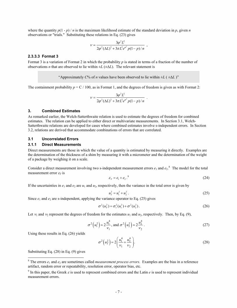
where the quantity p(1 - p) / n is the maximum likelihood estimate of the standard deviation in p, given n observations or "trials." Substituting these relations in Eq. (23) gives
2
2 2
2 2 2
3
2 ( ) 3 (1 ) /
L
L L e p p
n
,
2.3.3.3 Format 3
Format 3 is a variation of Format 2 in which the probability p is stated in terms of a fraction of the number of observations n that are observed to lie within ±L (±L). The relevant statement is
“Approximately C% of n values have been observed to lie within ±L ( ±L )”
The containment probability p = C / 100, as in Format 1, and the degrees of freedom is given as with Format 2:
2
2 2
2 2 2
3
2 ( ) 3 (1 ) /
L
L L e p p
n
2
.
3. Combined Estimates
As remarked earlier, the Welch-Satterthwaite relation is used to estimate the degrees of freedom for combined estimates. The relation can be applied to either direct or multivariate measurements. In Section 3.1, Welch-Satterthwaite relations are developed for cases where combined estimates involve s-independent errors. In Section 3.2, relations are derived that accommodate combinations of errors that are correlated. 3.1 Uncorrelated Errors
3.1.1 Direct Measurements
Direct measurements are those in which the value of a quantity is estimated by measuring it directly. Examples are the determination of the thickness of a shim by measuring it with a micrometer and the determination of the weight of a package by weighing it on a scale. Consider a direct measurement involving two s-independent measurement errors e1 and e2.
8 The model for the total measurement error T is 1T e e .9 (24)
If the uncertainties in e1 and e2 are u1 and u2, respectively, then the variance in the total error is given by
2 21Tu u u2
2 . (25)
Since e1 and e2 are s-independent, applying the variance operator to Eq. (25) gives
. (26) 2 2 2 2 2 21 1 2( ) ( ) ( )Tu u u
Let 1 and 2 represent the degrees of freedom for the estimates u1 and u2, respectively. Then, by Eq. (9),
4 4
2 2 2 211 2
1 2
2 , and 2u
u u 2u
. (27)
Using these results in Eq. (26) yields
4 4
2 2 1 2
1 2
2Tu u
u
. (28)
Substituting Eq. (28) in Eq. (9) gives
8 The errors e1 and e2 are sometimes called measurement process errors. Examples are the bias in a reference artifact, random error or repeatability, resolution error, operator bias, etc. 9 In this paper, the Greek is used to represent combined errors and the Latin e is used to represent individual measurement errors.
- 7 -
4
4 41 2
1 2
Tu
u u
, (29)
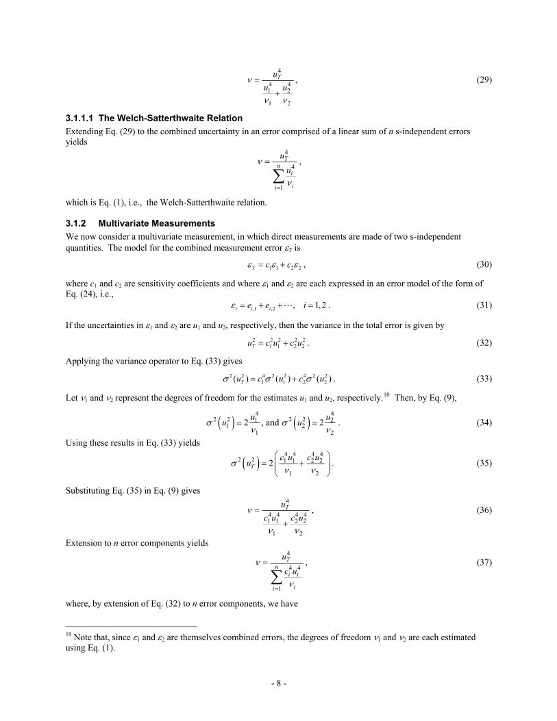
3.1.1.1 The Welch-Satterthwaite Relation
Extending Eq. (29) to the combined uncertainty in an error comprised of a linear sum of n s-independent errors yields
4
4
1
Tn
i
ii
u
u
,
which is Eq. (1), i.e., the Welch-Satterthwaite relation. 3.1.2 Multivariate Measurements
We now consider a multivariate measurement, in which direct measurements are made of two s-independent quantities. The model for the combined measurement error T is
1 1 2 2T c c , (30)
where c1 and c2 are sensitivity coefficients and where 1 and 2 are each expressed in an error model of the form of Eq. (24), i.e., ,1 ,2 , 1,i i ie e i 2 . (31)
If the uncertainties in 1 and 2 are u1 and u2, respectively, then the variance in the total error is given by
. (32) 2 2 2 21 1 2 2Tu c u c u 2
Applying the variance operator to Eq. (33) gives
. (33) 2 2 4 2 2 4 2 21 1 2 2( ) ( ) ( )Tu c u c u
Let 1 and 2 represent the degrees of freedom for the estimates u1 and u2, respectively.10 Then, by Eq. (9),
4 4
2 2 2 211 2
1 2
2 , and 2u
u u 2u
. (34)
Using these results in Eq. (33) yields
4 4 4 4
2 2 1 1 2 2
1 2
2Tc u c u
u
. (35)
Substituting Eq. (35) in Eq. (9) gives
4
4 4 4 41 1 2 2
1 2
Tu
c u c u
, (36)
Extension to n error components yields
4
4 4
1
Tn
i i
ii
u
c u
, (37)
where, by extension of Eq. (32) to n error components, we have
10 Note that, since 1 and 2 are themselves combined errors, the degrees of freedom 1 and 2 are each estimated using Eq. (1).
- 8 -
2 2
1
n
T ii
u c
2iu
2
2
2 2
.
3.2 Correlated Errors
3.2.1 Direct Measurements
Consider now a case where the measurement error T is the sum of two errors, as in Eq. (24), whose respective standard deviations are u1 and u2 and whose correlation coefficient is 12. The variance in the total error is given by
. (38) 2 2 21 2 12 12Tu u u u u
From Eq. (38) and the “variance addition rule,” we have11
(39) 2 2 2 2 2 2 2 2
1 2 12 1 2
2 2 2 21 2 12 1 1 2 12 2 1 2
( ) ( ) ( ) 4 ( )
2cov( , ) 4 cov( , ) 4 cov( , ) .
Tu u u u u
u u u u u u u u
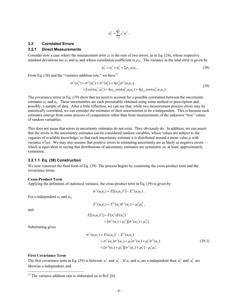
The covariance terms in Eq. (39) show that we need to account for a possible correlation between the uncertainty estimates u1 and u2. These uncertainties are each presumably obtained using some method or prescription and, possibly, a sample of data. After a little reflection, we can see that, while two measurement process errors may be statistically correlated, we can consider the estimates of their uncertainties to be s-independent. This is because such estimates emerge from some process of computation rather than from measurements of the unknown “true” values of random variaables. This does not mean that errors in uncertainty estimates do not exist. They obviously do. In addition, we can assert that the errors in the uncertainty estimates can be considered random variables, whose values are subject to the vagaries of available knowledge, so that each uncertainty estimate u is distributed around a mean value with variance 2(u). We may also assume that positive errors in estimating uncertainty are as likely as negative errors — which is equivalent to saying that distributions of uncertainty estimates are symmetric or, at least, approximately symmetric. 3.2.1.1 Eq. (39) Construction
We now construct the final form of Eq. (39) The process begins by examining the cross-product term and the covariance terms. Cross-Product Term Applying the definition of statistical variance, the cross-product term in Eq. (39) is given by
2 21 2 1 2 1 2( ) [( ) ] ( )u u E u u E u u .
For s-independent u1 and u2,
2 2 21 2 1 2 1 2( ) ( ) ( )E u u E u E u ,
and 2 2 2
1 2 1 2
2 2 21 1 2 2
[( ) ] ( ) ( )
[ ( ) ][ ( ) ].
E u u E u E u
u u 2
Substituting gives
(39.1)
2 2 21 2 1 2 1 2
2 2 2 2 2 21 2 2 1 1
2 2 2 2 2 21 1 2 2 1 2
( ) ( ) ( )
( ) ( ) ( ) ( )
[ ( ) ][ ( ) ] .
u u E u u E u u
u u u u
u u
2
First Covariance Term The first covariance term in Eq. (39) is between and . If u1 and u2 are s-independent then and are
likewise s-independent, and
21u 2
2u 21u 2
2u
11 The variance addition rule is elaborated on in Ref. [6].
- 9 -
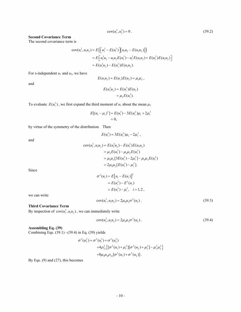
2 21 2cov( , ) 0u u . (39.2)
Second Covariance Term The second covariance term is
2 2 21 1 2 1 1 1 2 1 2
3 2 2 21 2 1 2 1 1 1 2 1 1 2
3 21 2 1 1 2
cov( , ) ( ) ( )
( ) ( ) ( ) ( )
( ) ( ) ( ).
u u u E u E u u u E u u
E u u u u E u u E u u E u E u u
E u u E u E u u
For s-independent u1 and u2, we have
1 2 1 2 1 2( ) ( ) ( )E u u E u E u ,
and 3 31 2 1 2
32 1
( ) ( ) (
( ).
E u u E u E u
E u
)
3
To evaluate , we first expand the third moment of u1 about the mean 1 31( )E u
3 3 21 1 1 1 1 1[( ) ] ( ) 3 ( ) 2
0,
E u E u E u
by virtue of the symmetry of the distribution. Then
3 21 1 1( ) 3 ( ) 2E u E u 3
1 ,
and 2 3 21 1 2 1 2 1 1 2
3 22 1 1 2 1
2 21 2 1 1 1 2 1
2 21 2 1 1
cov( , ) ( ) ( ) ( )
( ) ( )
[3 ( ) 2 ] ( )
2 [ ( ) ].
u u u E u u E u E u u
E u E u
E u E u
E u
2
2
2
Since
22
2 2
2 2
( ) ( )
( ) ( )
( ) , 1,2 ,
i i i
i i
i i
u E u E u
E u E u
E u i
we can write . (39.3) 2
1 1 2 1 2 1cov( , ) 2 ( )u u u u Third Covariance Term By inspection of , we can immediately write 2
1 1 2cov( , )u u u
. (39.4) 22 1 2 1 2 2cov( , ) 2 ( )u u u u
Assembling Eq. (39) Combining Eqs. (39.1) –(39.4) in Eq. (39) yields
2 2 2 2 2 2
1 2
2 2 2 2 2 2 212 1 1 2 2 1 2
2 21 2 12 1 2
( ) ( ) ( )
4 [ ( ) ][ ( ) ]
8 [ ( ) ( )] .
Tu u u
u u
u u
By Eqs. (9) and (27), this becomes
- 10 -
4 42 2 1 2
1 2
2 2 2 2 2 2 212 1 1 2 2 1 2
2 21 2 12 1 2
( ) 2 2
4 [ ( ) ][ ( ) ]
8 [ ( ) ( )] .
T
u uu
u u
u u
. (40)
Our best estimates for the distribution mean values 1 and 2 are the uncertainty estimates u1 and u2, respectively, and we write Eq. (40) as
4 4
2 2 2 2 2 2 2 2 2 2 21 212 1 1 2 2 1 2 1 2 12 1 2
1 2
( ) 2 2 4 [ ( ) ][ ( ) ] 8 [ ( ) ( )]T
u uu u u u u u u u u
u u
3.2.1.2 The Effective Degrees of Freedom
Using this expression we can write a Welch-Satterthwaite relation for the degrees of freedom of a total uncertainty estimate for a combined error comprised of the sum of n measurement process errors in which two or more are correlated. By Eq. (9), we have
4
1 142 2 2 2 2 2 2 2 2
1 1 1
2 [ ( ) ][ ( ) ] 4 [ ( ) (
Tn n n n n
iij i i j j i j ij i j i j
ii i j i i j i
u
uu u u u u u u u u u
)]
, (41)
where is determined from , given in Eq. (38), and, 2(ui), i = 1, 2,…, n is given in Eq. (22), for Type B
estimates and is obtained for Type A estimates from Eq. (20) as
4Tu 2
Tu12
2
2
2i
ii
uu
. (42)
If it is desired to work with the degrees of freedom for both Type A and Type B estimates, then we can employ the observed degrees of freedom for Type A and the computed degrees of freedom for Type B estimates in Eq. (42). If so, then Eq. (41) can be written
4
2 21 14 2 22
1 1 1
12
2
Tn n n n n
j ji i iij i j ij i j
i i j ii i j i i j i
u
u uu u uu u
j
. (43)
3.2.2 Multivariate Measurements
By Eq. (22) and by comparison of Eqs. (41) and (30), we can see, that Eq. (41) can be extended to give the effective degrees of freedom for a multivariate measurement with correlated error components
4
1 14 42 2 2 2 2 2 2 2 2 2 2 2 2
1 1 1
2 [ ( ) ][ ( ) ] 4 [ ( ) ( )]
Tn n n n n
i iij i j i i j j i j ij i j i j i i j j
ii i j i i j i
u
c uc c u u u u u u c c u u c u c u
, (44)
where, by extension of Eqs. (32) and (38),
. (45) 1
2 2 2
1 1
2n n n
T i i ij i j ii i j i
u c u c c u
ju
Note that the degrees of freedom i for the ith uncertainty component ui, i = 1, 2, …, n, are computed using either Eq. (36), if the constituent errors of the ith component are s-independent, or Eq. (41) if correlations exist between constituent errors.
12 Substitution of Eq. (42) in Eq. (41) for both Type A and Type B estimates is made in Appendix B.
- 11 -
If it is desired to work with the degrees of freedom for both Type A and Type B estimates, then Eq. (44) can be written
4
2 21 14 4 2 2 22 2 2
1 1 1
12
2
Tn n n n n 2
j j ji i i i iij i j i j ij i j i j
i i j ii i j i i j i
u
u cc u u c uc c c c u u
j
u
. (46)
4. Conclusion
The Welch-Satterthwaite relation is used to compute the degrees of freedom for uncertainty estimates of combinations of s-independent errors. The relation is applicable whether the estimates are Type A, Type B or mixed. For the computed degrees of freedom to be useful in developing confidence limits or for other statistical uses, such as hypothesis testing, the degrees of freedom values for both Type A and Type B estimates must be developed in a rigorous way that quantifies the amount of knowledge available in developing the estimates. Obtaining the degrees of freedom for Type A estimates is straightforward. Typically, this has not been the case for Type B estimates. Nevertheless, valid Type B degrees of freedom estimates are obtainable through the use of appropriate methods. In this paper, such a method has been derived and embodied in three formats that facilitate its implementation. With regard to the Welch-Satterthwaite relation itself, its restricted applicability to combinations of s-independent errors has been found to be a drawback in cases where errors are correlated (see Appendix B). A method for overcoming this drawback has been presented, the result of which is a refinement of the Welch-Satterthwaite relation for cases involving combinations of correlated errors. References
[1] ANSI/NCSL Z540-2-1997 (R2002), U.S. Guide to the Expression of Uncertainty in Measurement (ISBN 1-58464-005-7). October 1997.
[2] Castrup, H., "Advanced Topics in Uncertainty Analysis," Tutorial, NCSLI 2005, Washington, D.C.
[3] Willink, R., “A generalization of the Welch–Satterthwaite formula for use with correlated uncertainty components,” Metrologia, 44, September 2007, pp. 340-349.
[4] Castrup, H., “Uncertainty Analysis for Risk Management,” Proc., Meas. Sci. Conf., Anaheim, January 1995.
[5] NCSLI, “Determining & Reporting Measurement Uncertainty,” Recommended Practice RP-12, Under Revision.
[6] NASA, “Measurement Uncertainty Analysis Principles and Methods,” NASA-HNBK-8739.19-3, 2009.
[7] Castrup, H., “Estimating Category B Degrees of Freedom,” Proc. Meas. Sci. Conf., Anaheim, January 2000.
[8] ISG, UncertaintyAnalyzer 3.0, © 2006-2009, Integrated Sciences Group, www.isgmax.com.
[9] ISG, Uncertainty Sidekick Pro, © 2006-2009, Integrated Sciences Group, www.isgmax.com.
[10] ISG, Type B Degrees of Freedom Calculator, © 1999-2004, Integrated Sciences Group, www.isgmax.com.
[11] ISG, Uncertainty Sidekick, © 2006-2009, Integrated Sciences Group, www.isgmax.com. Appendix A
The following presents the derivation of Eq. G3 of the GUM from Eq. (9). By Eq. (9),
4
2 22
( )
u
u
, (A-1)
and, by Eq. G3,
2
22 ( )
u
u
. (A-2)
- 12 -
As before, we work with the chi-square distributed variable 2 /y s2 , where s represent the standard deviation
computed for a sample of size n of a N(0, 2 ) variable x. Since x is N(0, 2
), the variable y is 2-distributed with = n – 1 degrees of freedom. The pdf is given by Eq. (4), repeated here for convenience
( 2)/2 /2
/2( )
22
yy ef y
. (A-3)
Then, as before,
2 2 /s y ,
and
/s y ,
with variance
2var( ) / vars y (A-4)
The variance of square root of y can be approximated using a first-order expansion, i.e.,
var var ( )
1 1var ( ) var[ ( )].
42
yy y
y
y yyy
(A-5)
By Eq. (6), var[ ( )] var( ) 2y y ,
and Eq. (A-5) becomes
var2
yy
.
Substituting this result in Eq. (A-4) gives
2
2
2 4
2 2 2
var( ) /2 2
.2 / 2
sy y
s s
If we now approximate with s and write var(s) as 2(s), we get
22 ( )
2
ss
,
which yields
2
22 ( )
s
s
. (A-6)
Generalizing this expression to apply to Type B as well as Type A estimates, we can write Eq. (A-6) as
2
22 ( )
u
u
,
which is Eq. G3 of the GUM.
- 13 -
Appendix B
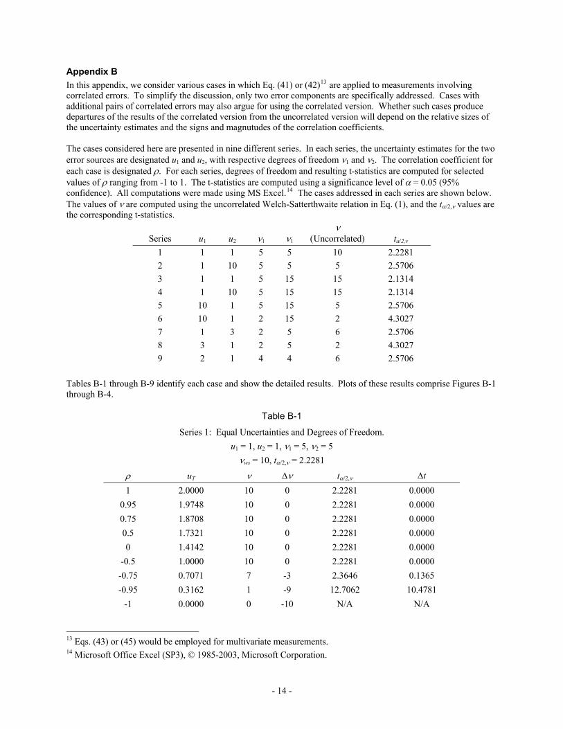
In this appendix, we consider various cases in which Eq. (41) or (42)13 are applied to measurements involving correlated errors. To simplify the discussion, only two error components are specifically addressed. Cases with additional pairs of correlated errors may also argue for using the correlated version. Whether such cases produce departures of the results of the correlated version from the uncorrelated version will depend on the relative sizes of the uncertainty estimates and the signs and magnutudes of the correlation coefficients. The cases considered here are presented in nine different series. In each series, the uncertainty estimates for the two error sources are designated u1 and u2, with respective degrees of freedom 1 and 2. The correlation coefficient for each case is designated . For each series, degrees of freedom and resulting t-statistics are computed for selected values of ranging from -1 to 1. The t-statistics are computed using a significance level of = 0.05 (95% confidence). All computations were made using MS Excel.14 The cases addressed in each series are shown below. The values of are computed using the uncorrelated Welch-Satterthwaite relation in Eq. (1), and the t/2, values are the corresponding t-statistics.
Series u1 u2 1 1
Uncorrelated) ta/2,v
1 1 1 5 5 10 2.2281
2 1 10 5 5 5 2.5706
3 1 1 5 15 15 2.1314
4 1 10 5 15 15 2.1314
5 10 1 5 15 5 2.5706
6 10 1 2 15 2 4.3027
7 1 3 2 5 6 2.5706
8 3 1 2 5 2 4.3027
9 2 1 4 4 6 2.5706
Tables B-1 through B-9 identify each case and show the detailed results. Plots of these results comprise Figures B-1 through B-4.
Table B-1
Series 1: Equal Uncertainties and Degrees of Freedom.
u1 = 1, u2 = 1, 1 = 5, 2 = 5ws = 10, t/2, = 2.2281
uT t/2, t
1 2.0000 10 0 2.2281 0.0000
0.95 1.9748 10 0 2.2281 0.0000
0.75 1.8708 10 0 2.2281 0.0000
0.5 1.7321 10 0 2.2281 0.0000
0 1.4142 10 0 2.2281 0.0000
-0.5 1.0000 10 0 2.2281 0.0000
-0.75 0.7071 7 -3 2.3646 0.1365
-0.95 0.3162 1 -9 12.7062 10.4781
-1 0.0000 0 -10 N/A N/A
13 Eqs. (43) or (45) would be employed for multivariate measurements. 14 Microsoft Office Excel (SP3), © 1985-2003, Microsoft Corporation.
- 14 -
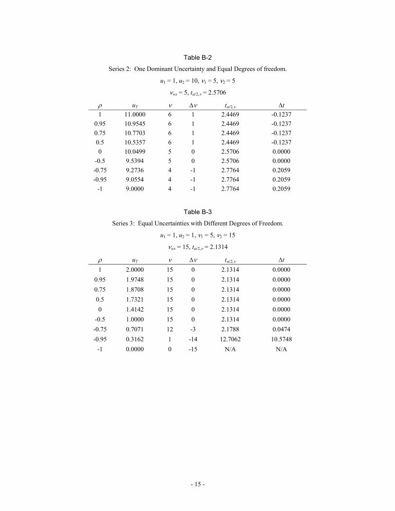
Table B-2
Series 2: One Dominant Uncertainty and Equal Degrees of freedom.
u1 = 1, u2 = 10, 1 = 5, 2 = 5
ws = 5, t/2, = 2.5706
uT t/2, t
1 11.0000 6 1 2.4469 -0.1237
0.95 10.9545 6 1 2.4469 -0.1237
0.75 10.7703 6 1 2.4469 -0.1237
0.5 10.5357 6 1 2.4469 -0.1237
0 10.0499 5 0 2.5706 0.0000
-0.5 9.5394 5 0 2.5706 0.0000
-0.75 9.2736 4 -1 2.7764 0.2059
-0.95 9.0554 4 -1 2.7764 0.2059
-1 9.0000 4 -1 2.7764 0.2059
Table B-3
Series 3: Equal Uncertainties with Different Degrees of Freedom.
u1 = 1, u2 = 1, 1 = 5, 2 = 15
ws = 15, t/2, = 2.1314
uT t/2, t
1 2.0000 15 0 2.1314 0.0000
0.95 1.9748 15 0 2.1314 0.0000
0.75 1.8708 15 0 2.1314 0.0000
0.5 1.7321 15 0 2.1314 0.0000
0 1.4142 15 0 2.1314 0.0000
-0.5 1.0000 15 0 2.1314 0.0000
-0.75 0.7071 12 -3 2.1788 0.0474
-0.95 0.3162 1 -14 12.7062 10.5748
-1 0.0000 0 -15 N/A N/A
- 15 -
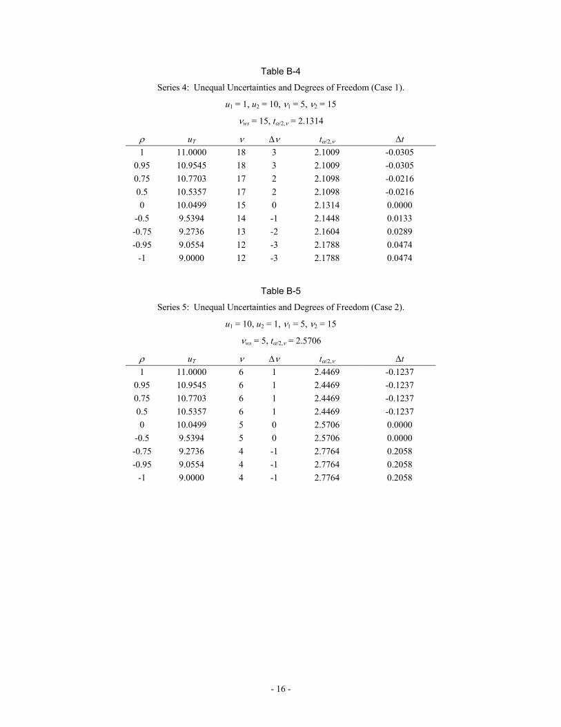
Table B-4
Series 4: Unequal Uncertainties and Degrees of Freedom (Case 1).
u1 = 1, u2 = 10, 1 = 5, 2 = 15
ws = 15, t/2, = 2.1314
uT t/2, t
1 11.0000 18 3 2.1009 -0.0305
0.95 10.9545 18 3 2.1009 -0.0305
0.75 10.7703 17 2 2.1098 -0.0216
0.5 10.5357 17 2 2.1098 -0.0216
0 10.0499 15 0 2.1314 0.0000
-0.5 9.5394 14 -1 2.1448 0.0133
-0.75 9.2736 13 -2 2.1604 0.0289
-0.95 9.0554 12 -3 2.1788 0.0474
-1 9.0000 12 -3 2.1788 0.0474
Table B-5
Series 5: Unequal Uncertainties and Degrees of Freedom (Case 2).
u1 = 10, u2 = 1, 1 = 5, 2 = 15
ws = 5, t/2, = 2.5706
uT t/2, t
1 11.0000 6 1 2.4469 -0.1237
0.95 10.9545 6 1 2.4469 -0.1237
0.75 10.7703 6 1 2.4469 -0.1237
0.5 10.5357 6 1 2.4469 -0.1237
0 10.0499 5 0 2.5706 0.0000
-0.5 9.5394 5 0 2.5706 0.0000
-0.75 9.2736 4 -1 2.7764 0.2058
-0.95 9.0554 4 -1 2.7764 0.2058
-1 9.0000 4 -1 2.7764 0.2058
- 16 -
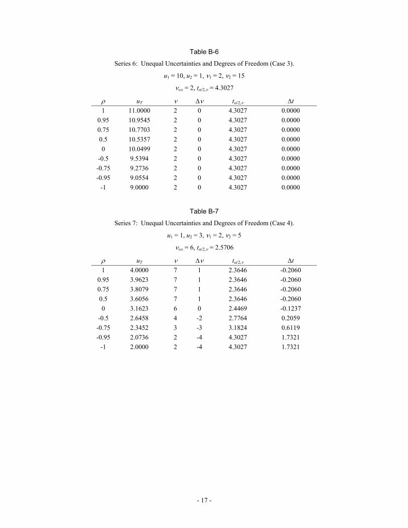
Table B-6
Series 6: Unequal Uncertainties and Degrees of Freedom (Case 3).
u1 = 10, u2 = 1, 1 = 2, 2 = 15
ws = 2, t/2, = 4.3027
uT t/2, t
1 11.0000 2 0 4.3027 0.0000
0.95 10.9545 2 0 4.3027 0.0000
0.75 10.7703 2 0 4.3027 0.0000
0.5 10.5357 2 0 4.3027 0.0000
0 10.0499 2 0 4.3027 0.0000
-0.5 9.5394 2 0 4.3027 0.0000
-0.75 9.2736 2 0 4.3027 0.0000
-0.95 9.0554 2 0 4.3027 0.0000
-1 9.0000 2 0 4.3027 0.0000
Table B-7
Series 7: Unequal Uncertainties and Degrees of Freedom (Case 4).
u1 = 1, u2 = 3, 1 = 2, 2 = 5
ws = 6, t/2, = 2.5706
uT t/2, t
1 4.0000 7 1 2.3646 -0.2060
0.95 3.9623 7 1 2.3646 -0.2060
0.75 3.8079 7 1 2.3646 -0.2060
0.5 3.6056 7 1 2.3646 -0.2060
0 3.1623 6 0 2.4469 -0.1237
-0.5 2.6458 4 -2 2.7764 0.2059
-0.75 2.3452 3 -3 3.1824 0.6119
-0.95 2.0736 2 -4 4.3027 1.7321
-1 2.0000 2 -4 4.3027 1.7321
- 17 -
Table B-8
Series 8: Unequal Uncertainties and Degrees of Freedom (Case 5).
u1 = 3, u2 = 1, 1 = 2, 2 = 5
ws = 2, t/2, = 4.3027
uT t/2, t
1 4.0000 3 1 3.1824 -1.1202
0.95 3.9623 3 1 3.1824 -1.1202
0.75 3.8079 3 1 3.1824 -1.1202
0.5 3.6056 3 1 3.1824 -1.1202
0 3.1623 2 0 4.3027 0.0000
-0.5 2.6458 2 0 4.3027 0.0000
-0.75 2.3452 1 -1 12.7062 8.4036
-0.95 2.0736 1 -1 12.7062 8.4036
-1 2.0000 1 -1 12.7062 8.4036
Table B-9
Series 9: Unequal Uncertainties and Degrees of Freedom (Case 6).
u1 = 2, u2 = 1, 1 = 4, 2 = 4
ws = 6, t/2, = 2.5706
uT t/2, t
1 3.0000 7 1 2.3646 -0.2060
0.95 2.9665 7 1 2.3646 -0.2060
0.75 2.8284 7 1 2.3646 -0.2060
0.5 2.6458 7 1 2.3646 -0.2060
0 2.2361 6 0 2.4469 -0.1237
-0.5 1.7321 4 -2 2.7764 0.2059
-0.75 1.4142 2 -4 4.3027 1.7321
-0.95 1.0954 1 -5 12.7062 10.1356
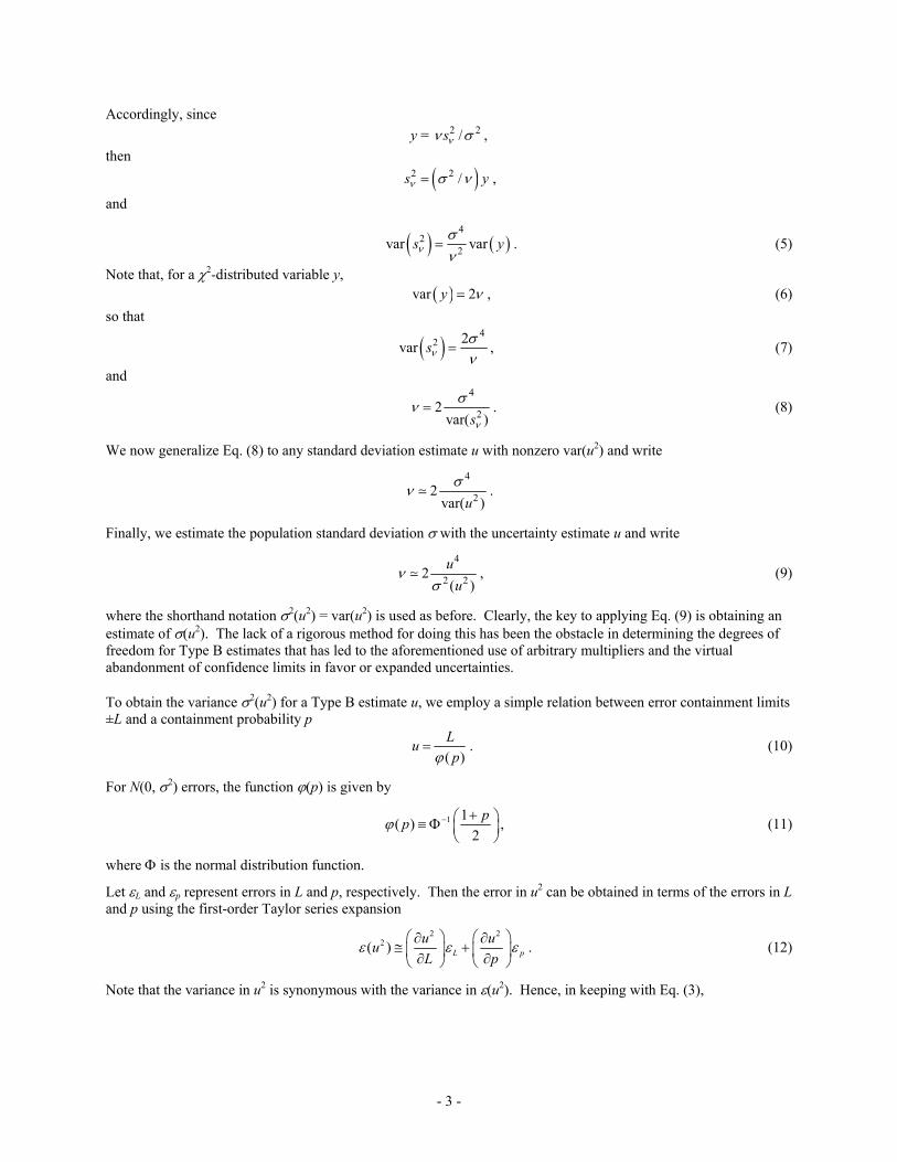
-1 1.0000 1 -5 12.7062 10.1356 While Tables B-1 through B-9 are informative, readers may derive additional insights from depictions of the results in graphic format. These depictions are provided below in Figures B-1 through B-4.
- 18 -
Series 1
Series 2 and 5Series 7
Series 3
Series 4
Series 9Series 8
Series 6
0
2
4
6
8
10
12
14
16
18
20
-1 -0.75 -0.5 -0.25 0 0.25 0.5 0.75 1
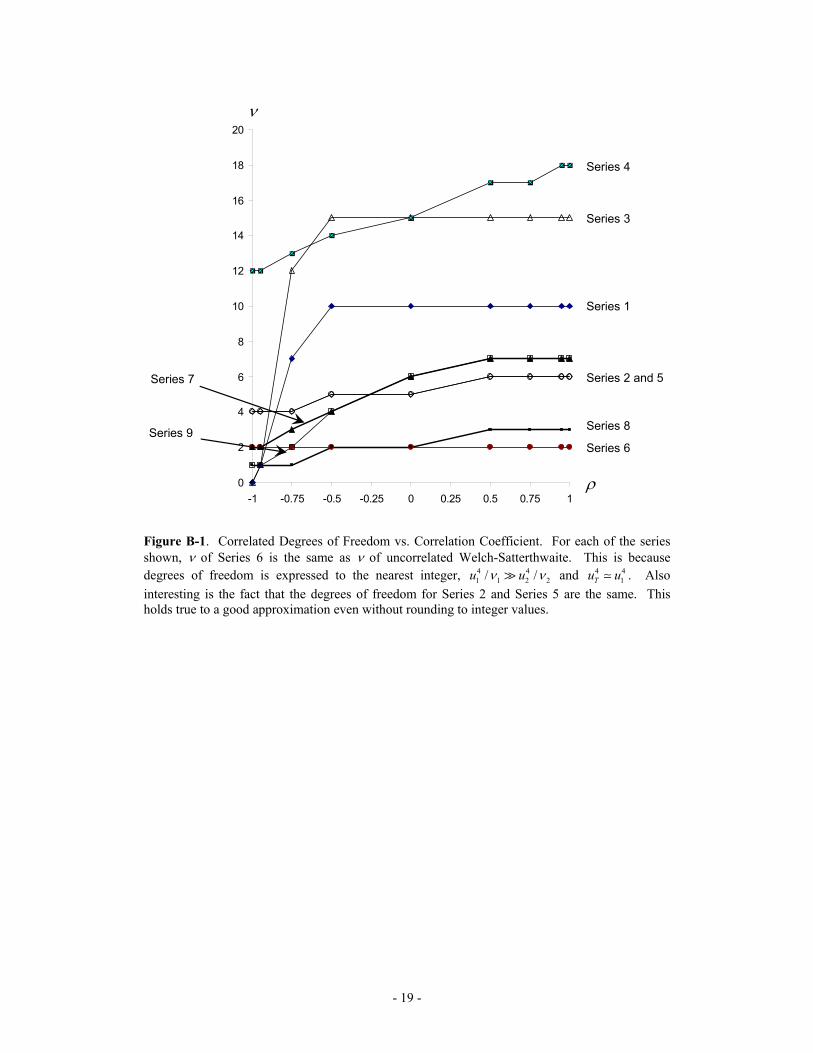
Figure B-1. Correlated Degrees of Freedom vs. Correlation Coefficient. For each of the series shown, of Series 6 is the same as of uncorrelated Welch-Satterthwaite. This is because degrees of freedom is expressed to the nearest integer, 4 4
1 1 2/u u 2/ and . Also
interesting is the fact that the degrees of freedom for Series 2 and Series 5 are the same. This holds true to a good approximation even without rounding to integer values.
41Tu u 4
- 19 -
-15
-14
-13
-12
-11
-10
-9
-8
-7
-6
-5
-4
-3
-2
-1
0
1
2
3
-1 -0.75 -0.5 -0.25 0 0.25 0.5 0.75 1
Series1
Series2
Series3
Series4
Series5
Series6
Series7
Series8
Series9
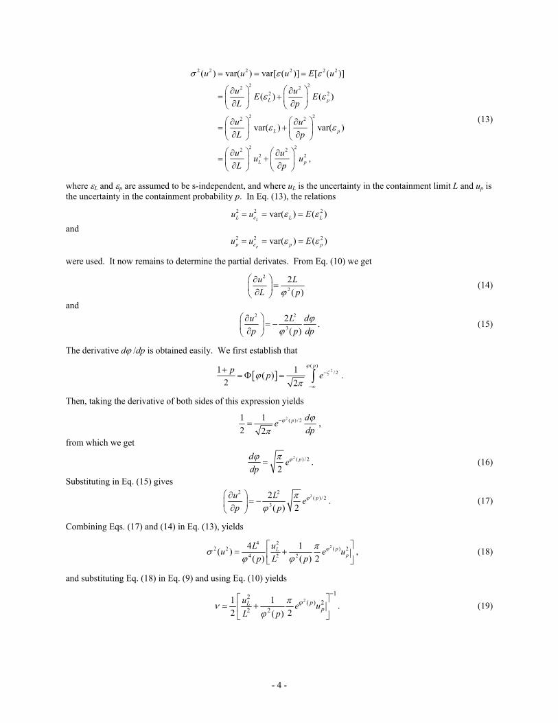
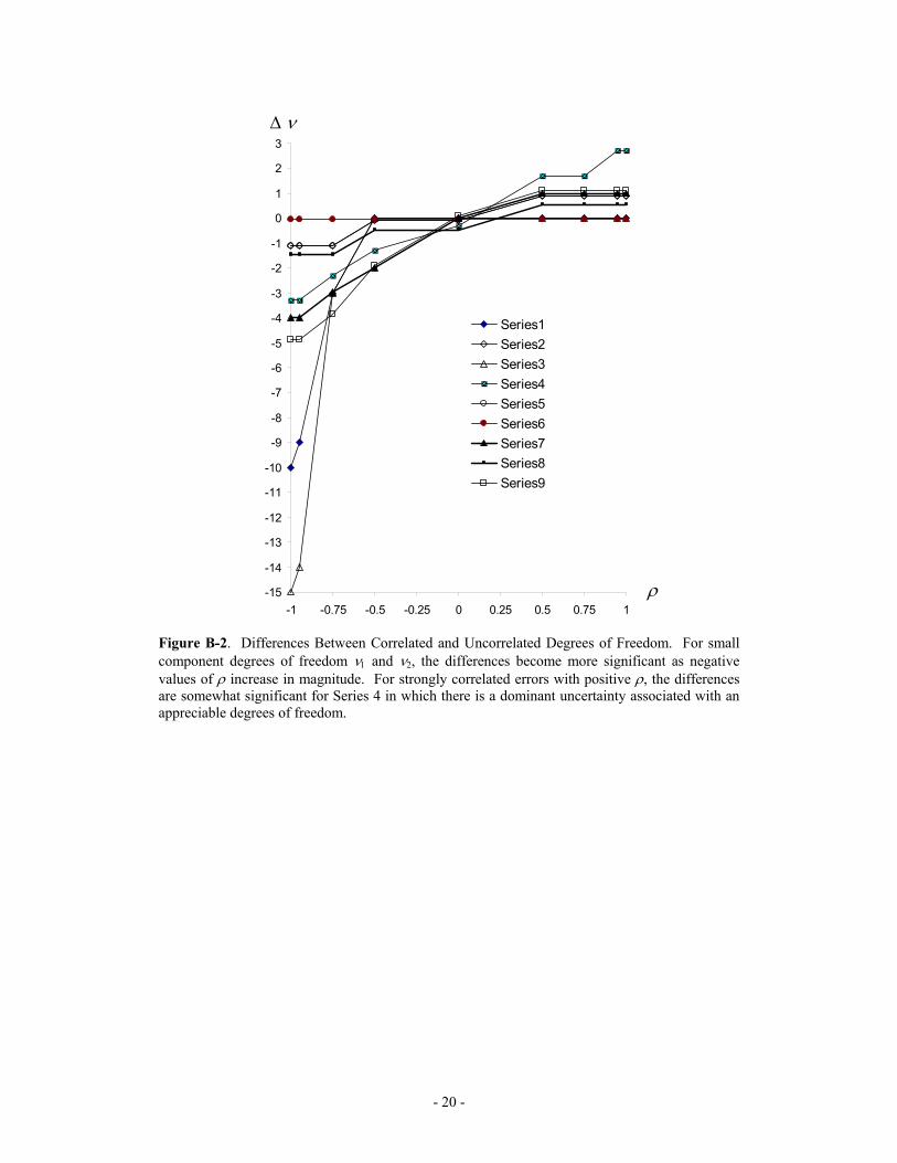
Figure B-2. Differences Between Correlated and Uncorrelated Degrees of Freedom. For small component degrees of freedom and , the differences become more significant as negative values of increase in magnitude. For strongly correlated errors with positive , the differences are somewhat significant for Series 4 in which there is a dominant uncertainty associated with an appreciable degrees of freedom.
- 20 -
t
1.00
2.00
3.00
4.00
5.00
6.00
7.00
8.00
9.00
10.00
11.00
12.00
13.00
-1 -0.75 -0.5 -0.25 0 0.25 0.5 0.75 1
Series1
Series2
Series3
Series4
Series5
Series6
Series7
Series8
Series9
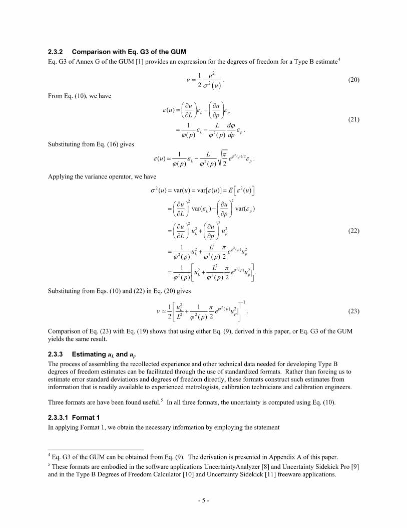
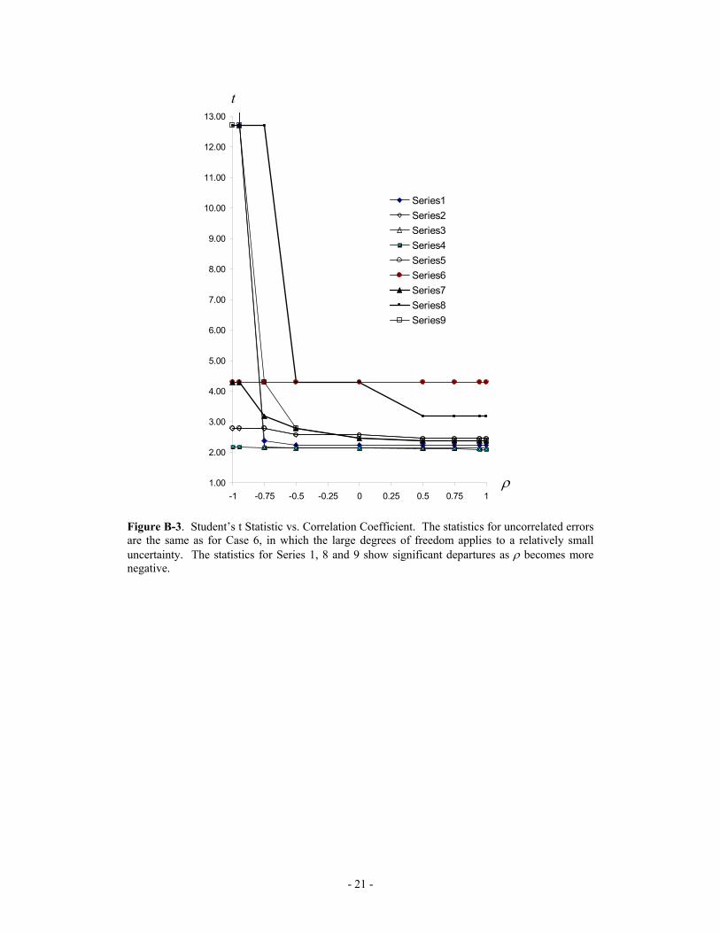
Figure B-3. Student’s t Statistic vs. Correlation Coefficient. The statistics for uncorrelated errors are the same as for Case 6, in which the large degrees of freedom applies to a relatively small uncertainty. The statistics for Series 1, 8 and 9 show significant departures as becomes more negative.
- 21 -
t
-2.00
-1.00
0.00
1.00
2.00
3.00
4.00
5.00
6.00
7.00
8.00
9.00
10.00
11.00
-1 -0.75 -0.5 -0.25 0 0.25 0.5 0.75 1
Series1
Series2
Series3
Series4
Series5
Series6
Series7
Series8
Series9
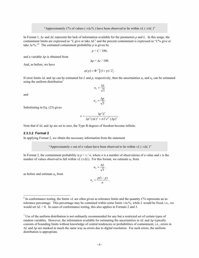
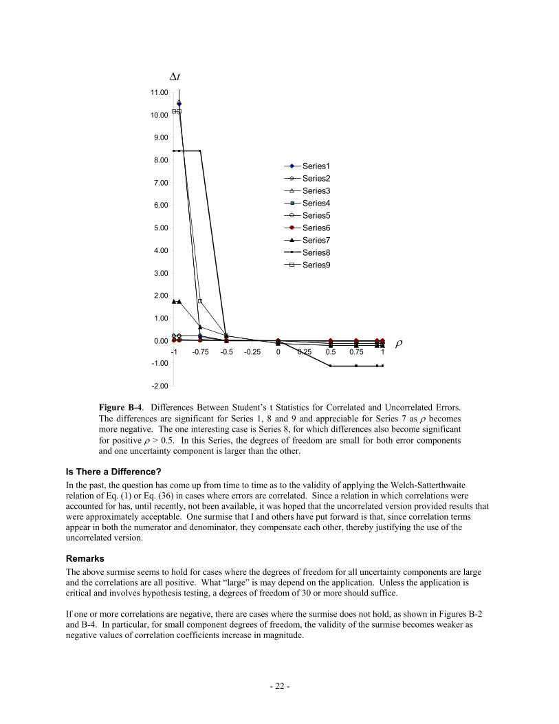
Figure B-4. Differences Between Student’s t Statistics for Correlated and Uncorrelated Errors. The differences are significant for Series 1, 8 and 9 and appreciable for Series 7 as becomes more negative. The one interesting case is Series 8, for which differences also become significant for positive > 0.5. In this Series, the degrees of freedom are small for both error components and one uncertainty component is larger than the other.
Is There a Difference?
In the past, the question has come up from time to time as to the validity of applying the Welch-Satterthwaite relation of Eq. (1) or Eq. (36) in cases where errors are correlated. Since a relation in which correlations were accounted for has, until recently, not been available, it was hoped that the uncorrelated version provided results that were approximately acceptable. One surmise that I and others have put forward is that, since correlation terms appear in both the numerator and denominator, they compensate each other, thereby justifying the use of the uncorrelated version. Remarks
The above surmise seems to hold for cases where the degrees of freedom for all uncertainty components are large and the correlations are all positive. What “large” is may depend on the application. Unless the application is critical and involves hypothesis testing, a degrees of freedom of 30 or more should suffice. If one or more correlations are negative, there are cases where the surmise does not hold, as shown in Figures B-2 and B-4. In particular, for small component degrees of freedom, the validity of the surmise becomes weaker as negative values of correlation coefficients increase in magnitude.
- 22 -
- 23 -
In addition, even for cases where the correlation coefficients are positive, the surmise does not hold if two or more errors are strongly correlated and there are dominant uncertainties associated with appreciable degrees of freedom. While the use of the uncorrelated version of the Welch-Satterthwaite relation is likely to be justified in many cases where correlations between errors exist, use of the correlated version seems to be appropriate under various circumstances, particularly those involving negative correlations. As we have seen, the advisability of using the correlated version is affected by whether correlations are negative. We may ask if such correlations are encountered in practice. The answer is “yes” in cases where difference measurements are made. A provincial example is determining whether differences between the diameter of a cannonball and the bore of a cannon are acceptable for desired performance. Other examples encountered in testing and calibration can be found. It would seem, then, that the recommended approach is to use the correlated version if correlations are present. One argument against this is that the correlated version is more complicated than the uncorrelated version. However, once the appropriate algorithm is embedded in computer code or a spreadsheet application, who cares, unless perhaps they work in a cave on a remote island without a laptop or electricity to run it?