A web service based tool to plan atmospheric research ... · 1 Introduction 1 2 First steps with the Mission Support User Interface1 ... our module using the netcdf4-python package7,

Supplementary document to

“A web service based tool to plan atmospheric research flights”

Basic usage and implementation of the Mission Support System

Marc Rautenhaus

Deutsches Zentrum fur Luft- und Raumfahrt, Institut fur Physik der Atmosphare

Oberpfaffenhofen, Germany

July 2011

A web service based tool to plan atmospheric research flights – basic usage and implementation

Contents

1 Introduction 1

2 First steps with the Mission Support User Interface 1

2.1 Starting the MSUI . . . . . . . . . . . . . . . . . . . . . . . . . . . . . . . . . . . . . . . . 1

2.2 Editing a flight track . . . . . . . . . . . . . . . . . . . . . . . . . . . . . . . . . . . . . . . 2

2.3 Loading forecast imagery from the Web Map Service . . . . . . . . . . . . . . . . . . . . . 3

3 Implementation of the Mission Support System 4

3.1 Open-source implementation using Python . . . . . . . . . . . . . . . . . . . . . . . . . . . 4

3.2 Web Map Service . . . . . . . . . . . . . . . . . . . . . . . . . . . . . . . . . . . . . . . . . 5

3.2.1 Implementation overview . . . . . . . . . . . . . . . . . . . . . . . . . . . . . . . . 5

3.2.2 Batch imagery . . . . . . . . . . . . . . . . . . . . . . . . . . . . . . . . . . . . . . 7

3.2.3 Modules . . . . . . . . . . . . . . . . . . . . . . . . . . . . . . . . . . . . . . . . . . 8

3.3 Mission Support User Interface . . . . . . . . . . . . . . . . . . . . . . . . . . . . . . . . . 10

3.3.1 Implementation overview . . . . . . . . . . . . . . . . . . . . . . . . . . . . . . . . 10

3.3.2 Modules . . . . . . . . . . . . . . . . . . . . . . . . . . . . . . . . . . . . . . . . . . 12

1 Introduction

This supplementary document extends the main article “A web service based tool to plan atmospheric

research flights” by providing usage guidelines for and implementation details of the Mission Support

System (MSS). Sect. 2 provides a description of the basic functionality of the Mission Support User

Interface (MSUI) for first-time users of the application. Sect. 3 introduces the implementation structure

of the MSS. Section 3.2 covers the MSS Web Map Service (WMS), Sect. 3.3 the MSUI. Both sections

first give an overview of the implementation, then list details of the implemented modules.

2 First steps with the Mission Support User Interface

This section introduces the basic functionality of the Mission Support User Interface and describes

how a flight plan can be drafted with the application. In the following, we assume a successful installation;

installation notes for deployment of both WMS and MSUI on Linux platforms are provided with the

source code.

2.1 Starting the MSUI

The start-up script for the user interface application is called startmss. It does not provide any

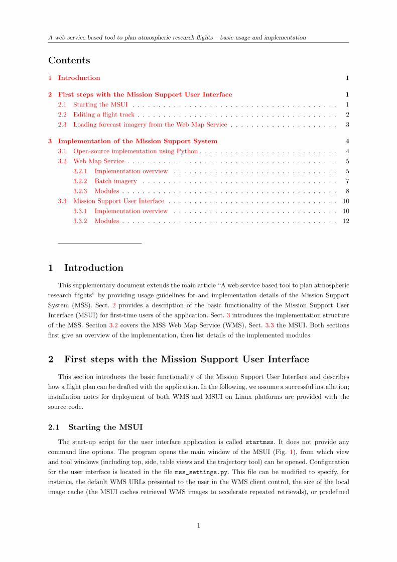
command line options. The program opens the main window of the MSUI (Fig. 1), from which view

and tool windows (including top, side, table views and the trajectory tool) can be opened. Configuration

for the user interface is located in the file mss_settings.py. This file can be modified to specify, for

instance, the default WMS URLs presented to the user in the WMS client control, the size of the local

image cache (the MSUI caches retrieved WMS images to accelerate repeated retrievals), or predefined

1


Figure 1: Screenshot of the Mission Support User Interface main window. New view windows can beopened from the “Views” menu. The application can open multiple flight tracks, however, only oneflight track can be edited at a time. Use the “set selected flight track active” button to edit an opentrack.

locations that the user can select in the table view. A number of options influencing the appearance of

the displayed plots and flight tracks (colours etc.) can be set directly in the application user interface.

2.2 Editing a flight track

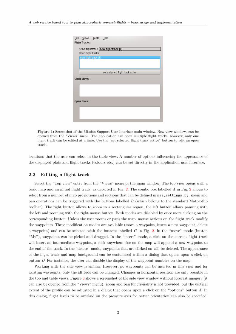
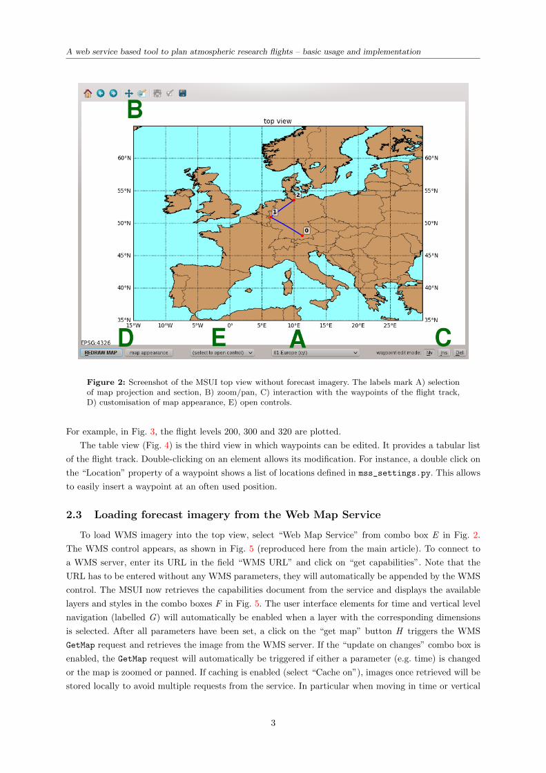
Select the “Top view” entry from the “Views” menu of the main window. The top view opens with a

basic map and an initial flight track, as depicted in Fig. 2. The combo box labelled A in Fig. 2 allows to

select from a number of map projections and sections that can be defined in mss_settings.py. Zoom and

pan operations can be triggered with the buttons labelled B (which belong to the standard Matplotlib

toolbar). The right button allows to zoom to a rectangular region, the left button allows panning with

the left and zooming with the right mouse button. Both modes are disabled by once more clicking on the

corresponding button. Unless the user zooms or pans the map, mouse actions on the flight track modify

the waypoints. Three modification modes are available (move a waypoint, insert a new waypoint, delete

a waypoint) and can be selected with the buttons labelled C in Fig. 2. In the “move” mode (button

“Mv”), waypoints can be picked and dragged. In the “insert” mode, a click on the current flight track

will insert an intermediate waypoint, a click anywhere else on the map will append a new waypoint to

the end of the track. In the “delete” mode, waypoints that are clicked on will be deleted. The appearance

of the flight track and map background can be customised within a dialog that opens upon a click on

button D. For instance, the user can disable the display of the waypoint numbers on the map.

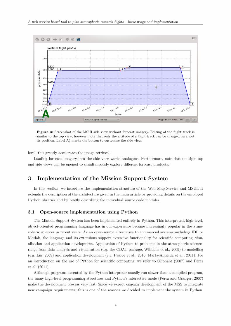
Working with the side view is similar. However, no waypoints can be inserted in this view and for

existing waypoints, only the altitude can be changed. Changes in horizontal position are only possible in

the top and table views. Figure 3 shows a screenshot of the side view window without forecast imagery (it

can also be opened from the “Views” menu). Zoom and pan functionality is not provided, but the vertical

extent of the profile can be adjusted in a dialog that opens upon a click on the “options” button A. In

this dialog, flight levels to be overlaid on the pressure axis for better orientation can also be specified.

2


Figure 2: Screenshot of the MSUI top view without forecast imagery. The labels mark A) selectionof map projection and section, B) zoom/pan, C) interaction with the waypoints of the flight track,D) customisation of map appearance, E) open controls.

For example, in Fig. 3, the flight levels 200, 300 and 320 are plotted.

The table view (Fig. 4) is the third view in which waypoints can be edited. It provides a tabular list

of the flight track. Double-clicking on an element allows its modification. For instance, a double click on

the “Location” property of a waypoint shows a list of locations defined in mss_settings.py. This allows

to easily insert a waypoint at an often used position.

2.3 Loading forecast imagery from the Web Map Service

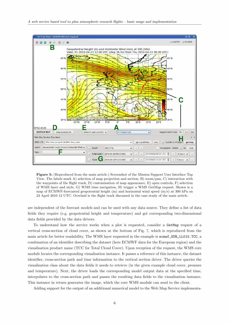
To load WMS imagery into the top view, select “Web Map Service” from combo box E in Fig. 2.

The WMS control appears, as shown in Fig. 5 (reproduced here from the main article). To connect to

a WMS server, enter its URL in the field “WMS URL” and click on “get capabilities”. Note that the

URL has to be entered without any WMS parameters, they will automatically be appended by the WMS

control. The MSUI now retrieves the capabilities document from the service and displays the available

layers and styles in the combo boxes F in Fig. 5. The user interface elements for time and vertical level

navigation (labelled G) will automatically be enabled when a layer with the corresponding dimensions

is selected. After all parameters have been set, a click on the “get map” button H triggers the WMS

GetMap request and retrieves the image from the WMS server. If the “update on changes” combo box is

enabled, the GetMap request will automatically be triggered if either a parameter (e.g. time) is changed

or the map is zoomed or panned. If caching is enabled (select “Cache on”), images once retrieved will be

stored locally to avoid multiple requests from the service. In particular when moving in time or vertical

3


Figure 3: Screenshot of the MSUI side view without forecast imagery. Editing of the flight track issimilar to the top view, however, note that only the altitude of a flight track can be changed here, notits position. Label A) marks the button to customise the side view.

level, this greatly accelerates the image retrieval.

Loading forecast imagery into the side view works analogous. Furthermore, note that multiple top

and side views can be opened to simultaneously explore different forecast products.

3 Implementation of the Mission Support System

In this section, we introduce the implementation structure of the Web Map Service and MSUI. It

extends the description of the architecture given in the main article by providing details on the employed

Python libraries and by briefly describing the individual source code modules.

3.1 Open-source implementation using Python

The Mission Support System has been implemented entirely in Python. This interpreted, high-level,

object-oriented programming language has in our experience become increasingly popular in the atmo-

spheric sciences in recent years. As an open-source alternative to commercial systems including IDL or

Matlab, the language and its extensions support extensive functionality for scientific computing, visu-

alisation and application development. Application of Python to problems in the atmospheric sciences

range from data analysis and visualisation (e.g. the CDAT package, Williams et al., 2009) to modelling

(e.g. Lin, 2009) and application development (e.g. Pascoe et al., 2010; Marta-Almeida et al., 2011). For

an introduction on the use of Python for scientific computing, we refer to Oliphant (2007) and Perez

et al. (2011).

Although programs executed by the Python interpreter usually run slower than a compiled program,

the many high-level programming structures and Python’s interactive mode (Perez and Granger, 2007)

make the development process very fast. Since we expect ongoing development of the MSS to integrate

new campaign requirements, this is one of the reasons we decided to implement the system in Python.

4


Figure 4: Screenshot of the MSUI table view. Waypoints can be inserted and deleted, coordinatesand flight levels for the individual waypoints can be directly edited. Waypoint locations can be given aname, the “comments” field allows the user to store additional remarks along with a waypoint. Here,the latitude value of waypoint 2 has just been changed.

Additional reasons are the wide range of available libraries making Python suitable for many tasks

from replacing shell scripts to designing graphical user interfaces and web applications, the option to

include time-critical methods implemented in a compiled language, and that Python and its libraries are

open-source.

The major extension libraries we use include NumPy (van der Walt et al., 2011) and SciPy1 for data

processing, Matplotlib with its basemap toolkit (Hunter, 2007; Tosi, 2009) for visualisation, and PyQt4

(Summerfield, 2007) for the graphical user interface.

3.2 Web Map Service

3.2.1 Implementation overview

The WMS module has been implemented as a WSGI (Web Server Gateway Interface2) application

using the PASTE toolkit3. It can thus be run with the PASTE HTTP-server, or be integrated into an

Apache4 installation. Prediction data are transferred from ECMWF to DLR via ftp and converted from

GRIB to CF-compliant NetCDF5 with Unidata’s NetCDF Java library6. The resulting files are read in

our module using the netcdf4-python package7, plotting is done with Matplotlib.

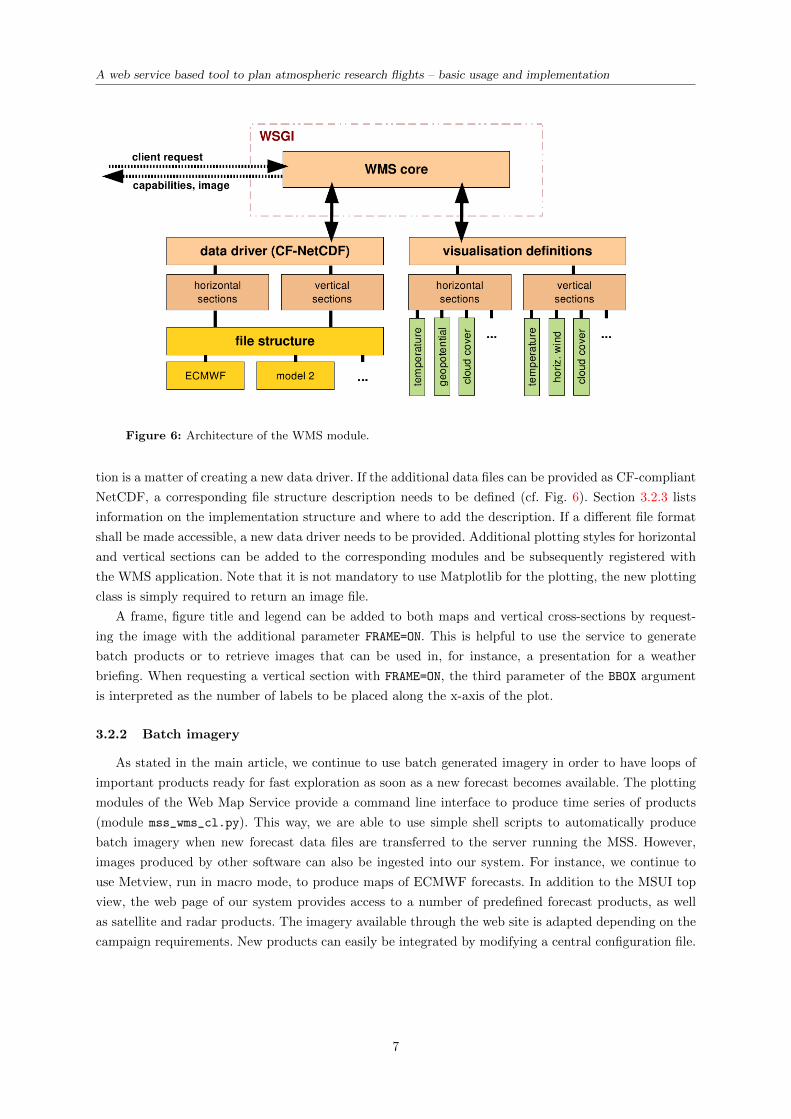
The architecture is based on the concept of separating data access and plotting logic (Fig. 6). The

core module, implementing the WSGI handler, keeps instances of data driver classes responsible for

loading and interpolating NWP data, and to visualisation classes defining the WMS layers that are

available by the service. For both data drivers and visualisations, a corresponding superclass providing

common methods is subclassed to implement methods specific to horizontal map sections and vertical

cross-sections. Should other data types be required at a later time (for example, vertical profiles or time

series), additional subclasses can be defined. The data drivers can locate the data files they need to open

through a set of classes describing the file structure of the available prediction data. For each forecast

model registered with the WMS, one such class describes how the model output dataset is organised.

This modularity allows for straightforward integration of additional datasets. The visualisation classes

1http://www.scipy.org2http://www.wsgi.org3http://pythonpaste.org4http://httpd.apache.org5http://cf-pcmdi.llnl.gov6http://www.unidata.ucar.edu/software/netcdf-java7http://code.google.com/p/netcdf4-python

5

http://www.scipy.org

http://www.wsgi.org

http://pythonpaste.org

http://httpd.apache.org

http://cf-pcmdi.llnl.gov

http://www.unidata.ucar.edu/software/netcdf-java

http://code.google.com/p/netcdf4-python


Figure 5: (Reproduced from the main article.) Screenshot of the Mission Support User Interface TopView. The labels mark A) selection of map projection and section, B) zoom/pan, C) interaction withthe waypoints of the flight track, D) customisation of map appearance, E) open controls, F) selectionof WMS layer and style, G) WMS time navigation, H) trigger a WMS GetMap request. Shown is amap of ECMWF-forecasted geopotential height (m) and horizontal wind speed (m/s) at 300 hPa on23 April 2010 12 UTC. Overlaid is the flight track discussed in the case study of the main article.

are independent of the forecast models and can be used with any data source. They define a list of data

fields they require (e.g. geopotential height and temperature) and get corresponding two-dimensional

data fields provided by the data drivers.

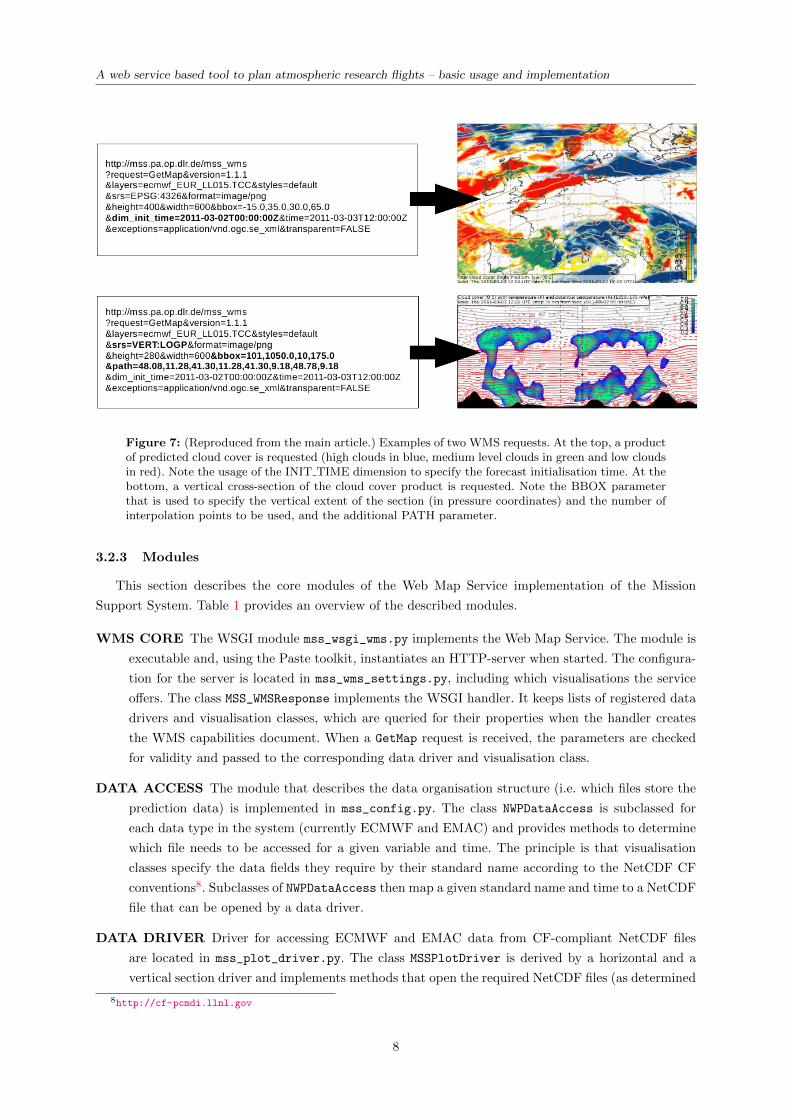
To understand how the service works when a plot is requested, consider a GetMap request of a

vertical cross-section of cloud cover, as shown at the bottom of Fig. 7, which is reproduced from the

main article for better readability. The WMS layer requested in the example is ecmwf_EUR_LL015.TCC, a

combination of an identifier describing the dataset (here ECMWF data for the European region) and the

visualisation product name (TCC for Total Cloud Cover). Upon reception of the request, the WMS core

module locates the corresponding visualisation instance. It passes a reference of this instance, the dataset

identifier, cross-section path and time information to the vertical section driver. The driver queries the

visualisation class about the data fields it needs to retrieve (in the given example cloud cover, pressure

and temperature). Next, the driver loads the corresponding model output data at the specified time,

interpolates to the cross-section path and passes the resulting data fields to the visualisation instance.

This instance in return generates the image, which the core WMS module can send to the client.

Adding support for the output of an additional numerical model to the Web Map Service implementa-

6


Figure 6: Architecture of the WMS module.

tion is a matter of creating a new data driver. If the additional data files can be provided as CF-compliant

NetCDF, a corresponding file structure description needs to be defined (cf. Fig. 6). Section 3.2.3 lists

information on the implementation structure and where to add the description. If a different file format

shall be made accessible, a new data driver needs to be provided. Additional plotting styles for horizontal

and vertical sections can be added to the corresponding modules and be subsequently registered with

the WMS application. Note that it is not mandatory to use Matplotlib for the plotting, the new plotting

class is simply required to return an image file.

A frame, figure title and legend can be added to both maps and vertical cross-sections by request-

ing the image with the additional parameter FRAME=ON. This is helpful to use the service to generate

batch products or to retrieve images that can be used in, for instance, a presentation for a weather

briefing. When requesting a vertical section with FRAME=ON, the third parameter of the BBOX argument

is interpreted as the number of labels to be placed along the x-axis of the plot.

3.2.2 Batch imagery

As stated in the main article, we continue to use batch generated imagery in order to have loops of

important products ready for fast exploration as soon as a new forecast becomes available. The plotting

modules of the Web Map Service provide a command line interface to produce time series of products

(module mss_wms_cl.py). This way, we are able to use simple shell scripts to automatically produce

batch imagery when new forecast data files are transferred to the server running the MSS. However,

images produced by other software can also be ingested into our system. For instance, we continue to

use Metview, run in macro mode, to produce maps of ECMWF forecasts. In addition to the MSUI top

view, the web page of our system provides access to a number of predefined forecast products, as well

as satellite and radar products. The imagery available through the web site is adapted depending on the

campaign requirements. New products can easily be integrated by modifying a central configuration file.

7


Figure 7: (Reproduced from the main article.) Examples of two WMS requests. At the top, a productof predicted cloud cover is requested (high clouds in blue, medium level clouds in green and low cloudsin red). Note the usage of the INIT TIME dimension to specify the forecast initialisation time. At thebottom, a vertical cross-section of the cloud cover product is requested. Note the BBOX parameterthat is used to specify the vertical extent of the section (in pressure coordinates) and the number ofinterpolation points to be used, and the additional PATH parameter.

3.2.3 Modules

This section describes the core modules of the Web Map Service implementation of the Mission

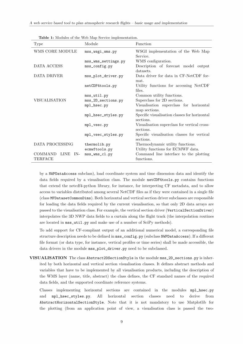
Support System. Table 1 provides an overview of the described modules.

WMS CORE The WSGI module mss_wsgi_wms.py implements the Web Map Service. The module is

executable and, using the Paste toolkit, instantiates an HTTP-server when started. The configura-

tion for the server is located in mss_wms_settings.py, including which visualisations the service

offers. The class MSS_WMSResponse implements the WSGI handler. It keeps lists of registered data

drivers and visualisation classes, which are queried for their properties when the handler creates

the WMS capabilities document. When a GetMap request is received, the parameters are checked

for validity and passed to the corresponding data driver and visualisation class.

DATA ACCESS The module that describes the data organisation structure (i.e. which files store the

prediction data) is implemented in mss_config.py. The class NWPDataAccess is subclassed for

each data type in the system (currently ECMWF and EMAC) and provides methods to determine

which file needs to be accessed for a given variable and time. The principle is that visualisation

classes specify the data fields they require by their standard name according to the NetCDF CF

conventions8. Subclasses of NWPDataAccess then map a given standard name and time to a NetCDF

file that can be opened by a data driver.

DATA DRIVER Driver for accessing ECMWF and EMAC data from CF-compliant NetCDF files

are located in mss_plot_driver.py. The class MSSPlotDriver is derived by a horizontal and a

vertical section driver and implements methods that open the required NetCDF files (as determined

8http://cf-pcmdi.llnl.gov

8

http://cf-pcmdi.llnl.gov


Table 1: Modules of the Web Map Service implementation.

Type Module Function

WMS CORE MODULE mss_wsgi_wms.py WSGI implementation of the Web MapService.

mss_wms_settings.py WMS configuration.DATA ACCESS mss_config.py Description of forecast model output

datasets.DATA DRIVER mss_plot_driver.py Data driver for data in CF-NetCDF for-

mat.netCDF4tools.py Utility functions for accessing NetCDF

files.mss_util.py Common utility functions.

VISUALISATION mss_2D_sections.py Superclass for 2D sections.mpl_hsec.py Visualisation superclass for horizontal

map sections.mpl_hsec_styles.py Specific visualisation classes for horizontal

sections.mpl_vsec.py Visualisation superclass for vertical cross-

sections.mpl_vsec_styles.py Specific visualisation classes for vertical

sections.DATA PROCESSING thermolib.py Thermodynamic utility functions.

ecmwftools.py Utility functions for ECMWF data.COMMAND LINE IN-TERFACE

mss_wms_cl.py Command line interface to the plottingfunctions.

by a NWPDataAccess subclass), load coordinate system and time dimension data and identify the

data fields required by a visualisation class. The module netCDF4tools.py contains functions

that extend the netcdf4-python library, for instance, for interpreting CF metadata, and to allow

access to variables distributed among several NetCDF files as if they were contained in a single file

(class MFDatasetCommonDims). Both horizontal and vertical section driver subclasses are responsible

for loading the data fields required by the current visualisation, so that only 2D data arrays are

passed to the visualisation class. For example, the vertical section driver (VerticalSectionDriver)

interpolates the 3D NWP data fields to a curtain along the flight track (the interpolation routines

are located in mss_util.py and make use of a number of SciPy methods).

To add support for CF-compliant output of an additional numerical model, a corresponding file

structure description needs to be defined in mss_config.py (subclass NWPDataAccess). If a different

file format (or data type, for instance, vertical profiles or time series) shall be made accessible, the

data drivers in the module mss_plot_driver.py need to be subclassed.

VISUALISATION The class Abstract2DSectionStyle in the module mss_2D_sections.py is inher-

ited by both horizontal and vertical section visualisation classes. It defines abstract methods and

variables that have to be implemented by all visualisation products, including the description of

the WMS layer (name, title, abstract) the class defines, the CF standard names of the required

data fields, and the supported coordinate reference systems.

Classes implementing horizontal sections are contained in the modules mpl_hsec.py

and mpl_hsec_styles.py. All horizontal section classes need to derive from

AbstractHorizontalSectionStyle. Note that it is not mandatory to use Matplotlib for

the plotting (from an application point of view, a visualisation class is passed the two-

9


dimensional data fields it requires and returns an image file with the corresponding plot).

AbstractHorizontalSectionStyle-derivative MPLBasemapHorizontalSectionStyle sets up a

Matplotlib Basemap instance and serves as superclass for the Matplotlib-based products described

here. The visualisation classes implementing the individual WMS layers hence are mainly

responsible for calling the appropriate plotting methods, for instance, contouring.

Vertical cross-sections are implemented in a similar manner in the modules mpl_vsec.py

and mpl_vsec_styles.py. A vertical visualisation class needs to inherit from

AbstractVerticalSectionStyle.

Additional visualisation classes for horizontal and vertical sections can be added to the modules

mpl_hsec_styles.py and mpl_vsec_styles.py, respectively. In mss_wms_settings.py, each vi-

sualisation class can be registered with datasets it shall visualise to create new WMS layers. Hence,

to make a new class accessible through the WMS, specify the NWPDataAccess instances that shall

be plottable by the class.

DATA PROCESSING The modules thermolib.py and ecmwftools.py implement a number of

methods for the manipulation of ECMWF data and the computation of common atmospheric

quantities (for instance, computation of equivalent potential temperature).

COMMAND LINE INTERFACE The executable module mss_wms_cl.py implements a command

line interface to access plotting functionality. The user can specify the plots to be generated by a

number of command line parameters. In addition to the WMS interface, specification of loops over

time and/or elevation is possible. The module can hence be used to create, for instance, a time

series of a vertical cross-section. It can also be called from shell scripts that trigger the generation

of batch products for the web page.

3.3 Mission Support User Interface

3.3.1 Implementation overview

The architecture of the MSUI is illustrated in Fig. 8, which is reproduced from the main article.

Similar to the Web Map Service module, the MSUI is built in a modular fashion. Recall from the main

article that the central elements are the views, application modules that allow the user to view a data

model, in particular the flight track, from different perspectives. Top, side and table view allow interacting

with the flight track. The loop view provides access to batch imagery. Tools are the modules that allow

to manage additional data models and that do not provide visualisations. For instance, we implemented

a trajectory tool that allows to load time series of past research flights and trajectory data from the

LAGRANTO model. A corresponding time series view provides the visualisation functionality.

The graphical user interface has been implemented with the PyQt4 bindings to Nokia’s Qt library.

We make use of a number of Qt mechanisms, for instance, signals and slots and the model-view-controller

concept (e.g. Summerfield, 2007, Chs. 4 and 14). This way, top, side and table view can provide syn-

chronised views of the flight track – if one waypoint is changed in one of the views, the other views are

automatically updated.

The implementation of the top view is based on the following principles: Plotting is implemented

with Matplotlib, which can directly be integrated into the PyQt4 user interface (Tosi, 2009, Ch. 6). A

subclass of the Basemap class (Matplotlib Basemap Toolkit) provides functionality exceeding Basemap’s

methods, for instance, to automatically draw the graticule, to redraw on zoom and pan and to manage

10


Figure 8: (Reproduced from the main article.) The architecture of the Mission Support User Interfaceapplication.

colour schemes. Interactive flight track elements have been realised with Matplotlib’s event handling

mechanisms9.

Two controls can be opened to load additional data into the view, a WMS client and a module to

load predicted satellite tracks obtained from the web-based NASA LaRC Satellite Overpass Predictor10.

Controls are modules that allow data from external sources to be loaded into a view. They are designed

as Qt widgets, so that they can be used in multiple views. The most complex control in the MSUI is the

WMS client. It is based on the OWSLib library11, which we modified to handle our WMS extensions

described in Sect. 3 of the main article. Retrieved images are loaded into the Python Imaging Library12

(PIL) and passed to Matplotlib. We also use PIL to store the images in a file cache in order to accelerate

the retrieval of already requested maps.

The side view is designed in a similar fashion to the top view, with Matplotlib used for plotting and

interactive modification of the waypoints and the WMS client control to retrieve cross-section imagery.

Exact coordinates and flight levels of the waypoints can be specified in the table view . In this module,

the flight planner can obtain information on the length of the flight track and its individual segments.

Furthermore, access to the flight performance web service is provided. The control implementing the

performance client reuses large parts of the code of the WMS client. Instead of WMS layer, style, and

time and elevation parameters, the user selects computation mode, aircraft configuration, time and

aircraft weight. Performance data returned by the Flight Performance Service are read by the control

and passed to the flight track data model, so they can be displayed to the user.

The loop view implements an image viewer to explore up to four loops of batch imagery. It thus

extends the functionality provided by the web site, in which two image loops can be displayed side-by-

side. In the loop view, all images are displayed synchronised in valid time, that is the images of all loops

9http://matplotlib.sourceforge.net/users/event_handling.html10http://www-air.larc.nasa.gov/tools/predict.htm11http://pypi.python.org/pypi/OWSLib/0.3.112http://www.pythonware.com/products/pil

11

http://matplotlib.sourceforge.net/users/event_handling.html

http://www-air.larc.nasa.gov/tools/predict.htm

http://pypi.python.org/pypi/OWSLib/0.3.1

http://www.pythonware.com/products/pil


are changed simultaneously. This includes forecasts from different initialisation times, so that subsequent

forecasts can be compared. For navigation, the user can use the mouse wheel to navigate in time and

use the mouse wheel with the shift key pressed to navigate in vertical elevation. Thus, by “scrolling”

through elevation, the loop view simplifies the exploration of the vertical structure of the forecasted

atmosphere. By means of the time synchronisation, a feature of interest can be conveniently tracked in

multiple forecast products (for example, a front in the equivalent potential temperature product, the

relative humidity product and the cloud product).

Functionality to load trajectory data and to display time series of the trajectories is implemented in

the trajectory tool and the time series view. The implementation follows the concept of encapsulating

data management logic in a tool and visualisation logic in a view. The trajectory tool allows to load

simulated particle trajectories from the LAGRANTO model as well as measurement data in NASA Ames

format13 (by using the NAppy package14). In addition to visualisation in the time series view, horizontal

tracks of the trajectories can be displayed in the top view, for instance, to visualise the movement of a

particular air mass.

The MSUI design allows new views or tools to be developed largely as stand-alone applications.

Depending on the purpose, the corresponding Qt signals have to be observed in order to communicate

with the flight track data model or other modules.

3.3.2 Modules

Analogous to Sect. 3.2.3, this section describes the core modules of the Mission Support User Interface

implementation. Table 2 provides an overview of the described modules.

MAIN The executable Python module mss_pyui.py implements the main window of the user interface

application. It manages view and tool windows (the user can open multiple windows) and provides

functionality to open, save, and switch between flight tracks.

SETTINGS The user interface configuration is contained in the module mss_settings.py, including

map projections, predefined URLs of WMS servers, cache settings and the configuration of the loop

view. The user can modify this module to customise the application.

FLIGHTTRACK Flight tracks are modelled by the WaypointsTableModel class in flighttrack.py,

a subclass of Qt’s QAbstractTableModel (thus following the model-view-controller concept). All

open views keep a reference to the currently active flight track data model, so that changes are

immediately synchronised. The flight track data model keeps a list of Waypoint instances that

describe the individual waypoints of the flight track. It also provides methods to store the waypoints

to and load them from an XML file. Distances between waypoints are computed by using the geopy

toolbox15. Results from a performance computation can be parsed. The performance service might

introduce additional waypoints in ascending and descending flight track segments, hence its results

are kept in a second list of waypoints. This way, the views can request the contents of either list,

depending on what shall be displayed to the user (currently only implemented for the table view).

VIEWS All views are derived from MSSViewWindow, contained in the module mss_qt.py. This super-

class provides methods to manage the displayed flight track model and control widgets.

13http://badc.nerc.ac.uk/help/formats/NASA-Ames14http://home.badc.rl.ac.uk/astephens/software/nappy15http://code.google.com/p/geopy

12

http://badc.nerc.ac.uk/help/formats/NASA-Ames

http://home.badc.rl.ac.uk/astephens/software/nappy

http://code.google.com/p/geopy


Table 2: Modules of the User Interface (MSUI) implementation.

Type Module Function

MAIN mss_pyui.py Main window of the user interface appli-cation.

SETTINGS mss_settings.py MSUI configuration.VIEWS mss_qt.py Superclass for view windows.

topview.py Top view user interface.sideview.py Side view user interface.tableview.py Table view user interface.loopview.py Loop view user interface.timeseriesview.py Time series view user interface.mpl_qtwidget.py Integration of Matplotlib canvas into Qt

user interface.mpl_map.py Map canvas for the top view.mpl_pathinteractor.py Interactive flight track elements for top

and side view.loopviewer_widget.py Loop view component displaying a single

time series of batch images.FLIGHTTRACK flighttrack.py Flight track data model.CONTROLS wms_control.py Control to access a WMS server.

satellite_control.py Control to load satellite track predictions.performance_control.py Control to access the flight performance

service.TOOLS trajectories_tool.py Tool to load NASA Ames files and LA-

GRANTO output data.lagranto_output_reader.py Utility functions to load LAGRANTO

output data.trajectory_item_tree.py Data model for trajectory data.

TOP VIEW The top view is implemented in topview.py. The class MSSTopViewWindow manages the

Qt elements of the graphical user interface. Map plotting functionality is implemented in a number

of classes. The underlying principle has been adapted from Tosi (2009, Ch. 6). We make use of Mat-

plotlib’s Qt4Agg backend for rendering. The Matplotlib class FigureCanvasQTAgg16 is inherited by

MplCanvas, which sets up a figure canvas and provides methods common to both horizontal and ver-

tical views. MplCanvas in turn is subclassed by MplTopViewCanvas. This class manages the Basemap

instance, the interactive flight track, WMS images and legends. The canvas class is embedded in

a Qt widget (MplTopViewWidget) that is an element of the top view GUI. MplTopViewWidget is

derived from MplNavBarWidget, which provides the Matplotlib typical navigation toolbar to zoom,

pan or save the plot. Canvas and widget classes are implemented in the module mpl_qtwidget.py.

As Matplotlib’s Basemap is primarily designed to produce static plots, we derived a class MapCanvas

to allow for a certain degree of interactivity (module mpl_map.py). MapCanvas extends Basemap

by functionality to, for instance, automatically draw a graticule. It also keeps references to plotted

map elements to allow the user to toggle their visibility, or to redraw when map section (zoom/pan)

or projection have been changed.

The flight track the user can interact with is implemented in the module mpl_pathinteractor.py.

WaypointsPath inherits from Matplotlib’s Path17 class and adds methods to insert and delete

vertices (in particular to find the correct insertion point of a new waypoint in the path), to syn-

16http://matplotlib.sourceforge.net/api/backend_qt4agg_api.html17http://matplotlib.sourceforge.net/api/path_api.html

13

http://matplotlib.sourceforge.net/api/backend_qt4agg_api.html

http://matplotlib.sourceforge.net/api/path_api.html


chronise with a flight track data model and to transform the waypoint coordinates to projection

coordinates. In particular, the subclass PathH_GC, which is used for the top view, connects the way-

points by means of great circles instead of straight lines. The class PathInteractor, for the top

view subclassed by HPathInteractor, implements the interactive editor for the path. It observes

both Matplotlib’s mouse events and Qt signals emitted when the flight track data model is changed

by another view and correspondingly updates a PathH_GC instance. The class also manages the plot

appearance of the path (i.e. colours and line styles).

WMS CLIENT The Web Map Service client control is implemented in the module wms_control.py.

The class WMSControlWidget manages the user interface and is used for both top and side

view, as functionality for both views only differs in what application actions are triggered

by a GetMap request. WMSControlWidget uses a subclass of the OWSLib WebMapService class

(MSSWebMapService, extending the OWSLib class by the WMS extensions described in the main

article for communication with the WMS server. The capabilities document returned by a WMS

is parsed by the OWSLib class, however, interpretation of, for instance, time values, is done by

WMSControlWidget. The central methods retrieveImage() and retrieveLegendGraphic() re-

trieve a specified WMS image and, if available, the corresponding legend. Requests are carried

out in separate threads in order to keep the GUI alive in the case of long response times. Im-

ages retrieved by both requests are cached on the local hard disk in files named by the MD5

hash value of the WMS request URL. Cache settings (size, maximum number of files) can be

configured in mss_settings.py. Support for basic HTTP authentication is provided (the user is

asked for user name and password should a server require these information). For the top view,

HSecWMSControlWidget implements the program logic that passes a retrieved image to the view’s

MapCanvas instance. Note that an image retrieval can be either triggered by clicking the “get map”

button (Fig. 5H, reproduced from the main article) or, if the “update on changes” check box is

enabled, by any GUI element changing the WMS parameters (including time and map section).

SATELLITE TRACKS The second control accessible from the top view is the satellite track

control implemented in satellite_control.py. It reads text files produced by the NASA

LaRC Satellite Overpass Predictor. The predicted satellite tracks are plotted on the map with

SatelliteOverpassPatch, implemented in mpl_map.py.

SIDE VIEW The side view (module sideview.py) is implemented in a similar manner to the top view.

The class MSSSideViewWindow manages the user interface. The Matplotlib canvas is implemented

in MplSideViewCanvas in mpl_qtwidget.py. It provides functionality to render the side view plot

(vertical axis, labelling of the x-axis with coordinate values) and manages WMS images and the

overlay of the flight levels lines. The WMS client widget is subclassed by VSecWMSControlWidget,

in which only layers offering the coordinate reference system VERT:LOGP are displayed to the user.

TABLE VIEW Module tableview.py accommodates the table view of the flight track. It contains a

QTableView instance that is registered with the flight track data model in flighttrack.py. The ta-

ble view uses the control PerformanceControlWidget, implemented in performance_control.py,

to access the flight performance service. The control reuses large parts of the WMS control. Re-

sults from the flight performance service are passed to the flight track data model. The table view

provides a button “view performance” to toggle the view between the two waypoint lists managed

by the flight track data model.

14


LOOP VIEW The loop view is implemented in the modules loopview.py and

loopviewer_widget.py. The class MSSLoopWindow manages the layout of the GUI. By using Qt’s

QSplitter, the user can modify the layout to view up to four instances of ImageLoopWidget.

This class implements the functionality to load batch imagery from an HTTP server. For a chosen

product, all available time steps and vertical levels are loaded. While this may require a large

amount of memory, it makes navigation through the images very fast. All images are stored with

a time stamp for time synchronisation. Similar to the WMS control, basic HTTP authentication

is supported to load the imagery. Maps are displayed in instances of LoopLabel, subclasses of

QLabel that observe mouse wheel events. When the mouse wheel is moved on top of one of the

displayed images, signals are emitted that notify all instances of ImageLoopWidget to synchronise

their images.

TRAJECTORY TOOL The modules trajectories_tool.py and timeseriesview.py accommo-

date the tool and view to load trajectory data and to display time series of the trajectories.

MSSTrajectoriesToolWindow implements the GUI to load trajectories. Flight tracks in NASA

Ames format are read by using the NAppy package, the module lagranto_output_reader.py

contains logic to read output from the LAGRANTO model. Loaded data are organised in a sub-

class of QAbstractItemModel (module trajectory_item_tree.py) and displayed to the user in

an instance of QTreeView. Elements selected in this tree view can be plotted either in a time series

view or in a top view. MapCanvas (mpl_map.py) provides the necessary methods to plot trajectories

on the map.

References

Hunter, J. D.: Matplotlib: A 2D Graphics Environment, Computing in Science and Engineering, 9, 90–95,doi:10.1109/MCSE.2007.55, 2007.

Lin, J. W. B.: qtcm 0.1.2: a Python implementation of the Neelin-Zeng Quasi-Equilibrium TropicalCirculation Model, Geoscientific Model Development, 2, 1–11, URL http://www.geosci-model-dev.

net/2/1/2009/, 2009.

Marta-Almeida, M., Ruiz-Villarreal, M., Otero, P., Cobas, M., Peliz, A., Nolasco, R., Cirano, M., andPereira, J.: OOF: A Python engine for automating regional and coastal ocean forecasts, EnvironmentalModelling & Software, 26, 680–682, doi:10.1016/j.envsoft.2010.11.015, 2011.

Oliphant, T. E.: Python for Scientific Computing, Computing in Science & Engineering, 9, 10–20, 2007.

Pascoe, S., Stephens, A., and Lowe, D.: Pragmatic service development and customisation with theCEDA OGC Web Services framework, EGU General Assembly 2010, held 2-7 May, 2010 in Vienna,Austria, p.9325, 12, 2010.

Perez, F. and Granger, B. E.: IPython: A System for Interactive Scientific Computing, Computing inScience and Engineering, 9, 21–29, doi:10.1109/MCSE.2007.53, 2007.

Perez, F., Granger, B. E., and Hunter, J. D.: Python: An Ecosystem for Scientific Computing, Computingin Science and Engineering, 13, 13–21, doi:10.1109/MCSE.2010.119, 2011.

Summerfield, M.: Rapid GUI Programming with Python and Qt (Prentice Hall Open Source SoftwareDevelopment), Prentice Hall, 1 edn., 2007.

Tosi, S.: Matplotlib for Python Developers, Packt Publishing, 2009.

van der Walt, S., Colbert, S. C., and Varoquaux, G.: The NumPy Array: A Structure for EfficientNumerical Computation, Computing in Science and Engineering, 13, 22–30, doi:10.1109/MCSE.2011.37, 2011.

15

http://www.geosci-model-dev.net/2/1/2009/

http://www.geosci-model-dev.net/2/1/2009/


Williams, D. N., Doutriaux, C. M., Drach, R. S., and McCoy, R. B.: The Flexible Climate Data Anal-ysis Tools (CDAT) for Multi-model Climate Simulation Data, Data Mining Workshops, InternationalConference on, 0, 254–261, doi:10.1109/ICDMW.2009.64, 2009.

16

Documents

A web service based tool to plan atmospheric research ... · 1 Introduction 1 2 First steps with the Mission Support User Interface1 ... our module using the netcdf4-python package7,