A water wave mixed type problem: existence of periodic ... · En este artículo establecemos un resultado de existencia de ondas periódicas para un sistema 2D del tipo Boussinesq

6

Rev. Acad. Colomb. Cienc. Ex. Fis. Nat. 39(150):6-17, enero-marzo de 2015

Matemáticas

Rev. Acad. Colomb. Cienc. 39(150): 6–17, enero–marzo de 2015

Matemáticas

A water wave mixed type problem: existence of periodictravelling waves for a 2D Boussinesq system

José R. Quintero∗

Departamento de Matemáticas, Universidad del Valle, Cali, Colombia

Abstract

In this paper we establish the existence of periodic travelling waves for a 2D Boussinesq type system in three-dimensional water-wave dynamics in the weakly nonlinear long-wave regime. For wave speed |c| > 1 and largesurface tension, we are able to characterize these solutions through spatial dynamics by reducing a linearly ill-posedmixed type initial value problem to a center manifold of finite dimension and infinite codimension. We will see thatthis center manifold contains all globally defined small-amplitude solutions of the travelling wave equation for theBoussinesq system that are periodic in the direction of propagation.

Key words: periodic travelling waves, center manifold approach, stability

Un problema de ondas de agua de tipo mixto: la existencia de ondas viajeras periódicas para un sistemaBoussinesq 2D

Resumen

En este artículo establecemos un resultado de existencia de ondas periódicas para un sistema 2D del tipo Boussinesqque describe la evolución de ondas de agua de gran elongación y pequeña ampitud que son débilmente lineales.Para velocidad de onda |c| > 1 y tensión superficial suficientemente grande, estas soluciones son caracterizadas através de dinámica espacial al reducir el problema de valor inicial (mal puesto a nivel lineal) a una variedad centralde dimensión finita y codimensión infinita. Se mostrará que dicha variedad central contiene todas las solucionesde onda viajera de pequenã amplitud para el sistema tipo Boussinesq que son periódicas en la dirección de propa-gación de la onda.

Palabras clave: ondas viajeras periódicas, método de variedad central, estabilidad.

1. IntroductionThis paper presents an existence result of nonlinear trav-elling water waves which are periodic in their directionof propagation and have a pulse structure in the un-bounded transverse spatial direction. As done for a widerange of applications, we use spatial dynamics and cen-ter manifold reduction to obtain such a result in a modelrelated with the water-wave problem. Here the expres-sion “spatial dynamics" means to perform a method inwhich a system of partial differential equations govern-ing a physical problem is formulated as a evolutionaryequation (in general ill-posed)

uζ = A(u) + G(u). (1.1)

in which an unbounded spatial coordinate plays the roleof the timelike variable ζ (see Kirchgässner (1982)). Inthis paper the method is applied to studying the ex-istence of non trivial periodic travelling wave for theBoussinesq type system related with the water waveproblem

⎧⎪⎪⎨⎪⎪⎩

ηt + �∇ ·�

η�

Φpx , Φp

y��

+ ΔΦ − μ6 Δ2Φ = 0,

Φt + η − μ�

σ − 12

�Δη + �

p+1

�Φp+1

x + Φp+1y

�= 0,

(1.2)where

√μ = h0/L is the ratio of undisturbed fluid depth

to typical wave length (long-wave parameter or disper-∗Correspondencia: J. R. Quintero: [email protected]. Recibido marzo 2014; aceptado diciembre 2014.

6

A water wave mixed type problem: existence of periodictravelling waves for a 2D Boussinesq system

A water wave mixed type problem

7

Rev. Acad. Colomb. Cienc. Ex. Fis. Nat. 39(150):6-17, enero-marzo de 2015Rev. Acad. Colomb. Cienc. 39(150): 6–17, enero–marzo de 2015 A water wave mixed type problem

sion coefficient), and � is the ratio of typical wave am-plitude to fluid depth (amplitude parameter or nonlin-earity coefficient), σ−1 is the Bond number (associatedwith the surface tension), Φ is the rescale nondimen-sional velocity potential on the bottom z = 0, and η is therescaled free surface elevation. We consider waves whichare periodic in a moving frame of reference, so that theyare periodic in the variable x − ct, where t denotes thetemporal variable. For this physical problem, we havea bounded spacelike coordinates (the vertical direction),which is bounded because the fluid has finite depth, andthe coordinate x − ct which is considered bounded be-cause we are looking for periodic wave in this variable.So, since there is not any restriction upon the behav-ior of the waves in the spatial direction y transverse totheir direction of propagation, we are allowed to use itas timelike variable. We apply spatial dynamics to theproblem by formulating this as an evolutionary systemof the form (1.1) with ζ = y in an infinite-dimensionalphase space consisting of periodic functions of x− ct (seeGrover & Schneider (2001), Sandstede & Scheel (1999),Sandstede & Scheel (2004), and Haragus-Courcelle &Schneider (1999) for applications to respectively non-linear wave equations, reaction-diffusion equations, andTaylor-Couette problems, and Quintero & Pego (2002)for periodic nonlinear travelling for the Benney–Lukemodel).In the case of wave speed |c| > 1 and bond numberσ > 1

2 , the Boussinesq system (1.2) under considera-tion in this paper has a very close relationship withthe Benney–Luke model derived in Quintero & Pego(1999) when a > b and also with the KP-II model(σ > 1

3 ), in the sense that travelling waves for the Boussi-nesq system (1.2) can generate travelling waves for theBenney–Luke model and the KP-II model, up to someorder. Event tough this fact, in the regime of wavespeed |c| > 1 and bond number σ > 1

2 , the Boussi-nesq system (1.2) seems to be closer to the linearizedsystem of the exact water wave problem with surface ten-sion (see Grover (2001), Grover & Mielke (2001)) sinceboth models share ill-posed spatial evolution equationswith finite-dimensional center manifolds, while for theBenney–Luke model in the same regime and also for theKP-II model there are ill-posed spatial evolution equa-tions with infinite-dimensional center manifolds.It is well known that a finite-dimensional dynamical sys-tem whose linear part has purely imaginary eigenval-ues admits an invariant manifold called the center mani-fold which contains all its small, bounded solutions. Thedimension of the center manifold is determined by thenumber of purely imaginary eigenvalues (e.g., see Van-derbauwhede (1989)). This type of results under specialhypotheses has been extended for infinite-dimensional

evolutionary systems whose linear part has either finiteor even infinite number of purely imaginary eigenvalues,showing in particular that the original problem is locallyequivalent to a system of ordinary differential equationswhose solutions can be expressed in terms of the solutionon the center space (tangent to the center manifold). Ageneralization regarding invariant manifolds of infinitedimension and codimension in nonautonomous systemswas obtained by Scarpellini (1990), but his hypothesesrequire that the operator A1 (A restricted to the hyper-bolic space) be bounded from H to H. We also have someworks by Mielke (1991) and Vanderbauwhede & Iooss(1982), Quintero & Pego (2002), among others. The gen-eral strategy of our proof will follow closely the linesof Vanderbauwhede (1989) (also see Quintero & Pego(2002), Kirchgässner (1982), Mielke (1988), Mielke(1992) for the case of a finite-dimensional center mani-fold in an ill-posed system for which the spectrum of A1is unbounded on both sides of the imaginary axis. Inorder to accomplish this, we need to transform the trav-elling wave system into an integral equation that mustcontain all small bounded solutions. By modifying thenonlinearity f outside a neighborhood of 0 using a cutofffunction, we are able to obtain an invariant local mani-fold as a consequence of the contraction mapping argu-ment.

The main differences between our results and those inVanderbauwhede & Iooss (1982) are that our cutoff oc-curs in a space with less regularity than the space regu-larity and also that the nonlinear part has a smoothingproperty. This facts are clever to control the norm ofsolutions in the right space using an indefinite energywhich turns out to be ”definite” on the center manifold.The stronger assumption on the nonlinear term f im-posed in the present work is completely natural for thepresent application to the Boussinesq system.

In this paper we describe all small travelling waves thattranslate steadily for σ > 1

2 with supercritical speed|c| > 1, which are periodic in the direction of transla-tion (or orthogonal to it). In this regime, after rescaling �and μ, the traveling-wave system for (1.2) takes the form⎛⎝ Δv − 1

6 Δ2v +∇ ·�

u�

vpx , vp

y��

− cux

u −�

σ − 12

�Δu + 1

p+1

�vp+1

x + vp+1y

�− cvx

⎞⎠ =

�00

�.

(1.3)Existence of periodic travelling waves follows by consid-

ering the system (1.3) as an evolution equation where yacts as the “time” variable. In this case when we seekfor x-periodic travelling wave solutions, the initial-valueproblem for the system (1.3) considered as an evolutionequation in the variable y has mixed type due to the factthat the Cauchy problem turns out to be linearly ill-posedfor wave speed |c| large enough and large bond number

7

Quintero JR

8

Rev. Acad. Colomb. Cienc. Ex. Fis. Nat. 39(150):6-17, enero-marzo de 2015Quintero JR Rev. Acad. Colomb. Cienc. 39(150): 6–17, enero–marzo de 2015

(σ > 12 ). To be more precise, at the linear level there

are finite many central modes (pure imaginary eigenval-ues) and infinitely many hyperbolic modes. As a conse-quence of this fact, the existence result of x-periodic trav-elling wave solutions involves using an invariant centermanifold of finite dimension and infinite codimension.This center manifold contains all globally defined small-amplitude solutions of the travelling wave equation forthe Boussinesq system that are x-periodic in the directionof propagation.

2. Periodic travelling waves for |c| > 1 andσ > 1

2

Recall that x-periodic travelling-wave profile (u, v)should satisfy the system (1.3). In order to look for theexistence of x-periodic travelling waves of period 2π, weset the new variables

u1 = ∂xv, u2 = ∂yv,

u3 = ∂yyv, u4 = ∂yyyv,

u5 = u, u6 = ∂yu,

then we have for γ�

σ − 12

�= 1 that

∂yu1 = ∂xu2, ∂yu2 = u3, ∂yu2 = u4 (2.4)

∂yu4 = 6∂xu1∂3xu1 + 6u3 − 2∂2

xu3 − 6c∂xu5+

6∂x(u5up1 ) + 6u6up

2 + 6pu5up−12 u3 (2.5)

∂yu5 = u6 (2.6)

∂yu6 = −cγu1 + γu5 − ∂2xu5+

+γ

p + 1

�up+1

1 + up+12

�(2.7)

In terms of the new variable Ut = (u1, u2, u3, u4, u5, u6),we see that this system can be rewritten as an evolutionin which y is considered as the time variable

∂yU = AU + G(U), (2.8)

where we have that

A =

⎛⎜⎜⎜⎜⎜⎜⎝

0 ∂x 0 0 0 00 0 I 0 0 00 0 0 I 0 0

6∂x − ∂3x 0 6I − ∂2

x 0 −6c∂x 00 0 0 0 0 I

−cγ 0 0 0 γ − 2∂2x 0

⎞⎟⎟⎟⎟⎟⎟⎠

and also

G(U) =

⎛⎜⎜⎜⎜⎜⎜⎜⎜⎝

000

6∂x(u5up1 ) + 6u6up

2 + 6pu5up−12 u3

0γ

p+1

�up+1

1 + up+12

�

⎞⎟⎟⎟⎟⎟⎟⎟⎟⎠

Now, for a given integer r ≥ 0, let Hr denote the Sobolevspace of 2π-periodic functions on R whose weak deriva-tives up to order k are square-integrable. Then Hr is aHilbert space with norm given by

�u�2Hk =

k∑j=0

� 2π

0|∂j

xu|2 dx

We will study the existence of x-periodic solutions for(2.8) in the Hilbert spaces H and X defined by

H = H1 × H1 × H0 × H−1, (2.9)

X = H2 × H2 × H1 × H0. (2.10)

Note that X is densely embedded in H. If we assumethat U(x; y) = ∑

n∈Z

�U(n, y)einx, then we see that

∂y �U(n) = �A(n) �U(n, y) + �Gn(U),

where the matrix �A(n) has the form

�A(n) =

⎛⎜⎜⎜⎜⎜⎜⎝

0 in 0 0 0 00 0 1 0 0 00 0 0 1 0 0

6in + in3 0 6 + 2n2 0 −6icn 00 0 0 0 0 1

−cγ 0 0 0 γ + 2n2 0

⎞⎟⎟⎟⎟⎟⎟⎠

It is straightforward to see that the characteristic polyno-mial P(n, β) of �A(n) is given by

P(n, β) = β6 − (6 + 3n2 + γ)β4 + [(6+ 2n2)(n2 + γ)

+ n2(6+ n2)]β2 + n2[6γc2 − (6 + n2)(n2 + γ)],(2.11)

where γ > 0, |c| > 0 and n ∈ Z. We note that the eigen-values for �A(n) are roots of the cubic polynomial pn inthe variable λ = β2 given by

pn(λ) = λ3 + a2(n)λ2 + a1(n)λ + a0(n), (2.12)

where a0(n), a1(n) and a2(n) are defined as

a2(n) = −(3n2 + 6 + γ) (2.13)

a1(n) = (6+ 2n2)(n2 + γ) + n2(6+ n2)

= 3n4 + 2(6+ γ)n2 + 6γ (2.14)

a0(n) = n2[6γc2 − (6 + n2)(n2 + γ)] (2.15)

= −n2[n4 + (6+ γ)n2 + 6γ(1− c2)]

8


9


Eigenvalues of A(n)

We want to compute the eigenvalues of A(n). Forn = 0, we have that a0(0) = 0, a1(0) = 6γ > 0,a2(0) = −(6 + γ) < 0 and the cubic equation (2.12) canbe easily solve since

λ3 − (6+ γ)λ2 + 6γλ = λ(λ2 − (6+ γ)λ + 6γ)

= λ(λ − γ)(λ − 6) = 0.

In other words, we have the existence of six eigenvaluesfor A(0) given by,

β1(0) = β2(0) = 0,

β3(0) =√

γ = −β4(0),

β5(0) =√

6 = −β6(0).

Assume now that n �= 0. We will see that for γ > 0and c2 > 1 large enough, the polynomial pn has a realroot λ1(n) which is negative for a finite number of n’sand positive for infinitely many n’s. To do this we needsomehow to localize the roots of the polynomial p�n forn �= 0. Note that

p�n(λ) = 3λ2 + 2a2(n)λ + a1(n)

has real roots given by

ρ+(n) = − a2(n)3

+

√a2

2(n)− 3a1(n)3

,

ρ−(n) = − a2(n)3

−√

a22(n)− 3a1(n)

3

since

a22(n)− 3a1(n) = γ2 − 6γ + 36 = (γ − 3)2 + 27 > 0.

Moreover, a direct computation shows that

pn(ρ±) =2a3

2(n)27

− a1(n)a2(n)3

+ a0(n)± 227

(3a1(n)

− a22(n))

√a2

2(n)− 3a1(n)

=2a3

2(n)27

− a1(n)a2(n)3

+ a0(n)

∓ 227

(γ2 − 6γ + 36)32

From this, we conclude for any n �= 0 that

pn(ρ−)− pn(ρ+) =427

(γ2 − 6γ + 36)32 > 0.

On the other hand, we have that

2a32(n)27

− a1(n)a2(n)3

+ a0(n)

=127

(162γc2n2 + 54γ(6+ γ)− 2(6+ γ)3

)

=127

(162γc2n2 − 2(6+ γ)(γ − 3)(γ − 12)

).

(2.16)

Using this we have that

pn(ρ±) =1

27

(162γc2n2 − 2(6+ γ)(γ − 3)(γ − 12)

∓2(γ2 − 6γ + 36)32

)

We set f (γ) = (γ2 − 6γ + 36)3 −((6+ γ)(γ − 3)(γ − 12))2 . We see that f (0) = f (6) = 0and that f �(0) = f �(6) = 0, so we have that

f (γ) = 35γ2(

γ2 − 6)2

> 0,

which implies that

(γ2 − 6γ + 36)32 > (6+ γ)(γ − 3)(γ − 12)

and so, we have for γ > 0 that

pn(ρ−) =1

27

(162γc2n2 + 2(γ2 − 6γ + 36)

32

−2(6+ γ)(γ − 3)(γ − 12)) >16227

γc2n2 > 0.

Now we note that

pn(ρ+) =1

27

(162γc2n2 − 2 ((6+ γ)(γ − 3)(γ − 12)

+(γ2 − 6γ + 36)32

)),

so, we have that pn(ρ+) is positive for |n| large and couldbe negative for a finite number of n’s. As a consequenceof this, for n �= 0 the polynomial pn has a real root λ1(n),whose sign depends on the sign of a0(n). In the casepn(ρ+) > 0, there are two conjugate complex roots λ2(n)and λ3(n) = λ2(n), and in the case pn(ρ+) < 0 there aretwo positive real root λ2(n) ≥ λ3(n) > 0. Finally, wewant to determine the sign of λ1(n) for γ > 0. We firstobserve for c2 > 1 large enough and γ > 0 that there isn0 �= 0 such that

a0(n) > 0 for 0 < n ≤ n0, and a0(n) < 0 for n > n0.

From this fact, we conclude for c2 > 1 large enough andγ > 0 that

λ1(n) < 0 for 0 < n ≤ n0, and λ1(n) > 0 for n > n0.

9

Quintero JR

10


Right and left eigenvectors of �A(n)

As we established above, β1(0) = β2(0) = 0 is an eigen-value. We see directly that the eigenvectors are

v1(0) = (1, 0, 0, 0, c, 0) t, v2(0) = (0, 1, 0, 0, 0, 0) t.

and left eigenvectors

z1(0) = (1, 0, 0, 0, c, 0) t, z2(0) = ((0, 1, 0,−1/6, 0, 0)t.

The eigenvalue β3(0) =√

γ = −β4(0) are single eigen-values with right eigenvectors

v3(0) = (0, 0, 0, 0, 1,√

γ)t, v4(0) = (0, 0, 0, 0, 1,−√γ)t.


z3(0) =1

2√

γ(c√

γ, 0, 0, 0,√

γ, 1)t,

z4(0) =−1

2√

γ(c√

γ, 0, 0, 0,−√γ, 1)t.

On the other hand, the eigenvalue β5(0) =√

6 = −β6(0)are single eigenvalues with right eigenvectors

v5(0) = (0, 1,√

6, 0, 1, 0)t, v6(0) = ((0, 1,−√6, 0, 1, 0)t.


z5(0) =112

(0, 0,√

6, 1, 0, 0)t,

z6(0) =112

(0, 0,−√6, 1, 0, 0)t.

Now, we will describe the form of the eigenvalues for�A(n) for n �= 0. In this case, we have that

β3(n) = −β4(n) =�

λ2(n) ∈ C,

β5(n) = −β6(n) =�

λ3(n) ∈ C

and for γ > 0 we have that

β1(n) = −β2(n) =�

λ1(n) ∈ iR, 0 ≤| n |≤ n0,

β1(n) = −β2(n) =�

λ1(n) ∈ R, | n |> n0.

A direct computation shows for 1 ≤ m ≤ 6 that βm(n) isa single eigenvalue with right eigenvector

vm(n) =�

in, βm(n), β2m(n), β3

m(n),

− cnγiΘm(n)

,− cnγβm(n)iΘm(n)

�t,

where Θm(n) = β2m(n)− (γ + n2). It is also straightfor-

ward to show that left eigenvector zm(n) is given by

zm(n) = Q(m, n)�

qm(n)inβm(n)

,qm(n)β2

m(n), βm(n), 1,

− cnβm(n)iΘm(n)

,− 6cniΘm(n)

�,

where qm(n) = β2m(n)(β2

m(n)− (6 + n2)) and Q(m, n) istaken such that

zm(n)vl(n) = δlm.

If we introduce the matrices Z(n) and V(n) given by

Z(n) =

⎛⎜⎜⎜⎜⎜⎜⎝

z1(n)z2(n)z3(n)z4(n)z5(n)z6(n)

⎞⎟⎟⎟⎟⎟⎟⎠

,

V(n) = (v1(n), v2(n), v3(n), v4(n), v5(n), v6(n)),

we have Z(n) · V(n) = I6 and

Z(n) �A(k)V(k) = diag (β1(n), β2(n), β3(n),β4(n), β5(n), β6(n)) , n ∈ Z.

Now, we observe that given any vector �U(n) ∈ R6, wemay write

�U(n) = V(n) · Z(n) �U(n) = V(n)U#(n),

where

U#(n) = Z(n)�U(n) =

⎛⎜⎜⎜⎜⎝

U#1(n)U#

2(n)U#

3(n)U#

4(n)U#

5(n)U#

6(n)

⎞⎟⎟⎟⎟⎠

.

Using this representation, we have for U = ∑n∈Z

�U(n)einx

that⎧⎪⎨⎪⎩

U = ∑n∈Z ∑6m=1 vm(n)U#

m(k)einx,

AU = ∑n∈Z ∑6m=1 βm(n)vm(n)U#

m(n)eikx.

(2.17)

We define the projections π0 and π1 for γ > 0 by

π0U = ∑0≤|n|≤n0

2

∑m=1

vm(n)U#m(k)einx (2.18)

π1U = ∑0≤|n|≤n0

6

∑m=3

vm(n)U#m(k)einx

+ ∑|n|>n0

6

∑m=1

vm(n)U#m(k)einx. (2.19)

10


11


We see directly from the explicit form of the roots ofthe polynomial pn that |βm(n)| grows asymptotically lin-early in |n|. In fact, we must recall that the roots λm(n)of �A(n) for 1 ≤ m ≤ 3 depend on the discriminant D(n)of pn defined as

D(n) = Q3(n) + R2(n).

where Q and R are defined by

Q(n) =3a1(n)− a2

2(n)9

R(n) =9a1(n)a2(n)− 27a0(n)− 2a3

2(n)54

More concretely, we have the following known result thatcharacterizes the roots for a cubic polynomial

1. if D(n) is positive, then pn has one real root(λ1(n)) and two are complex conjugates (λ2(n) andλ3(n) = λ2(n)).

2. if D(n) is negative, then pn has three different realroots, and

3. if D(n) = 0, then pn has three real roots, with twoof them are equal (λ2(n) = λ3(n)).

Moreover, the roots of the polynomial pn defined in(2.12) are explicitly given by

λ1 = −13

a2(n) + (S(n) + T(n)) (2.20)

λ2 = −13

a2(n)− 12(S(n) + T(n)) + i

√3

2(S(n) + T(n))

(2.21)

λ3 = −13

a2(n)− 12(S(n) + T(n))− i

√3

2(S(n) + T(n))

(2.22)

where S(n) and R(n) are numbers defined as

S(n) = 3

�R(n) +

�D(n), T(n) = 3

�R(n)−

�D(n),

such that S(n) + T(n) ∈ R and that S(n)− T(n) ∈ R forD(n) ≥ 0, and S(n) + T(n) ∈ R and that S(n)− T(n) ∈iR for D(n) < 0. In this particular case, we have forn �= 0 that

Q(n) = γ2 − 6γ + 369

= − (γ − 3)2 + 279

< 0

R(n) = −81γc2n2 + (6+ γ)(γ2 − 15γ + 36)27

.

Using this we see that Q(n) = O(1) and R(n) = O(n2)for |n| large enough, meaning that D(n) = O(n4) for |n|

large enough, and that |S(n)| = |T(n)| = O(n2) for |n|large enough. Using previous facts and formulas (2.20)-(2.22) for |n| large enough, we conclude for 1 ≤ m ≤ 3and |n| large enough

|λm(n)| � O(n2), (2.23)

and so, for |n| large enough and 1 ≤ m ≤ 6, we have that

|βm(n)| � O(|n|). (2.24)

Using this fact it is not difficult to verify that in termsof the coefficient vectors U#(n) we have the followingequivalence of norms:

⎧⎪⎨⎪⎩

�U�2H ∼ ∑n∈Z(1+ n2)2|U#(n)|2,

�U�2X ∼ ∑n∈Z(1+ n2)3|U#(n)|2.

(2.25)

From the equivalences in (2.25) it is evident that π0 andπ1 are bounded on H and on X with π0 + π1 = I, andit is clear that AXj ⊂ Hj where Xj = πjX and Hj = πj Hfor j = 0, 1. This yields the spectral decompositionsH = H0 ⊕ H1 and X = X0 ⊕ X1.

2.1. Center manifolds of finite dimension and infinitecodimension

Here we consider an abstract differential equations of theform

dudy (y) = Au(y) + f (u(y)). (2.26)

where X and H are Banach spaces with X densely em-bedded in H, A ∈ L(X, H), the space of bounded linearoperators from X to H, and f is continuously differen-tiable from H into H with f (0) = 0 and D f (0) = 0.We will assume that the nonlinear part f has the reg-ularizing effect: f (H) ⊂ X. This hypothesis on f is astronger condition than those imposed in many worksrelated with the existence center manifolds, but this com-pletely natural for the Boussinesq type system consid-ered in this paper. Existence of a local finite dimensionalcenter manifold can be established in the same fashionas the approach used in Quintero & Pego (2002) in thecase of having a center space with infinite dimension andinfinite codimension for the Benney–Luke model. As inthe later model, we must observe that the cutoff will beperformed in the H norm, and not in the X norm asin Quintero & Pego (2002). This is important since weneed to use an energy functional which is defined on H,which is conserved in time for classical solutions (takingvalues in X), but is indefinite in general. Fortunately forus, this energy controls the H norm for solutions on thecenter manifold. So, we require obtaining a center mani-fold that contains solutions with large X norm but smallH norm. This is a consequence that the nonlinearity fhas a smoothing property, mapping H into X.

11

Quintero JR

12


We will state the result for the existence of a locally in-variant center manifold of classical solutions for the sys-tem (2.26) under certain conditions which allow the cen-ter subspace (that associated with the purely imaginaryspectrum of A) to have finite dimension and infinite codi-mension. We start with some basic definitions and somehypotheses:

Definition 2.1. Let J ⊂ R be an open interval and u : R →H be a function. We say that u is a classical solution of (2.26)on J if the mapping y �→ u(y) is continuous from J into X, isdifferentiable from J into H and (2.26) holds for all y ∈ J.

Let β > 0, let Y and Z be Banach spaces and U be anopen set in Y. We define the Banach spaces Cb(U, Z),Lip(U, Z) and Yβ by

Cb(U, Z) :=

{f ∈ C(U, Z) : sup

u∈Z� f (u)�Z < ∞

}

Lip(U, Z) := { f ∈ C(U, Z) : � f (u)− f (v)�Z

≤ Mf �u − v�Y for all u, v ∈ U}Yβ := {u ∈ C(R, Y) : ||u||Yβ := sup

te−β|t|�u(t)�Y < ∞}.

Throughout this section we assume that there arebounded projections π0 and π1 on H such that

(i) (i) H = H0 ⊕ H1 with Hi := πi(H),

(ii) πi|X is bounded from X to X, and

(iii) AXi ⊆ Hi where Xi := πi(X), for i = 0, 1.

We see that equation (2.26) can be rewritten as the firstorder system

ddy u0(y) = A0u0(y) + π0 f (u(y)),

ddy u1(y) = A1u1(y) + π1 f (u(y)),

(2.27)

where Ai ∈ L(Xi, Hi) with Aiy = πi Ay for y ∈ Xi.We assume the following splitting properties for the op-erator A1, associated with the linear evolution equationdu/dy = Au.

(H1) There exists α > 0 and a positive function M1on [0, α) such that for any β ∈ [0, α) and for anyg1 ∈ C(R, X1) ∩ Hβ

1 the equation

ddy u1 = A1u1 + g1 (2.28)

has a unique solution in Hβ1 given by u1 = K1g1,

where K1 ∈ L(Hβ1 ) with �K1�L(Hβ

1 )≤ M1(β). Fur-

thermore �K1�L(Xβ1 )

≤ M1(β).

As done by J. Quintero and R. Pego in the case of theBenney–Luke model (see Quintero & Pego (2002)), weeasily have that

Theorem 2.1 (Local Center Manifold Theorem). Let H,X, A, π0, π1 and f be as above, and let

B(δ) = {y ∈ H0 : �y�H < δ}.

Then for all sufficiently small δ > 0 there exists φδ : H0 → X1such that

(i) φδ(0) = 0 and Dφδ(0) = 0.

(ii) φδ ∈ Cb(H0, X1)∩Lip(H0, X1), and on any ball B(δ�),φδ has Lipschitz constant L(δ�) satisfying L(δ�) < 1

2and L(δ�) → 0 as δ� → 0+.

(iii) The manifold Mδ ⊂ X given by

Mδ := {ξ + φδ(ξ) : ξ ∈ X0} (2.29)

is a local integral manifold for (2.26) over B(δ) ∩ X0.That is, given any y ∈ Mδ there is a continuous mapu : R → Mδ with u(0) = y, such that for any openinterval J containing 0 with π0u(J) ⊂ B(δ) it followsthat u is a classical solution of (2.26) on J. Moreover,u0 := π0u is the unique classical solution on J withu0(0) = π0y to the reduced equation

ddy u0(y) = A0u0(y) + Fδ(u0(y)), (2.30)

where Fδ : H0 → X0 is locally Lipschitz and is given byFδ(w) := π0 f (w + φδ(w)).

(iv) For any open interval J ⊂ R, every classical solu-tion u0 ∈ C1(J, H0) ∩ C(J, X0) of the reduced equation(2.30) such that u0(y) ∈ B(δ) for all y ∈ J yields, viau = u0 + φδ(u0), a classical solution u of the full equa-tion (2.26) on J.

(v) The manifold Mδ contains all classical solutions on R

that satisfy �u(y)�H ≤ δ for all y.

2.2. Linear dynamics analysis.

Now we are interested in establishing the solvabilityconditions to the linear level. First we consider thecenter subspace H0. We define the bounded C0-group{S0(y)}y∈R on H0 with infinitesimal generator A0 =A |X0 by

S0(y)U = ∑0≤|n|≤n0

2

∑m=1

vm(n)U#m(n)eβm(n)yeinx. (2.31)

12


13


Now, we want to determine the Green function to solvethe problem in the hyperbolic subspace H1. Let us con-sider the inhomogeneous linear equation

ddy U(t) = A1U(y) + G(y) (2.32)

where A1 = A|X1 . We need to observe that |�(λm(n)| ≥α > 0 for all n ∈ Z, except for m = 1, 2 when n �= 0.Let 0 ≤ � < α and let G ∈ C(R, X1) ∩ H�

1 , where for anyBanach space Y,

Y� = {u ∈ C(R, Y) | �u�Y� := supy

e−�|y|�u�Y < ∞}.

(2.33)Hereafter we will assume m and n are such that 1 ≤ m ≤6 and n ∈ Z \ {0}, or m = 5, 6 for n = 0. SupposeU ∈ C1(R, H1) ∩ C(R, X1) is a solution belonging to H�

1 .Then using the Fourier series expansion in x and multi-plying by the matrix Z(n) yields the differential equation

ddy U#

m(n, y) = βm(n)U#m(n, y) + G#

m(n, y) (2.34)

The functions G#m(n, ·) and U#

m(n, ·) belong to R� (Y = R

in (2.33)). From the fact that |βm(n)| ≥ α > �, we con-clude necessarily that

⎧⎪⎨⎪⎩

U#u(n, y) =

� y∞ eβu(k)(y−τ)G#

u(n, τ) dτ,

U#s (n, y) =

� y−∞ eβs(n)(y−τ)G#

s (n, τ) dτ.

(2.35)

where for 0 <| n |≤ n0 we have u = 3, 5 and s = 4, 6,and for | n |> n0 we have u = 1, 3, 5 and s = 2, 4, 6.As a direct consequence any solution of (2.32) in H�

1 isunique. We will see that the formulas (2.35) togetherwith the representation for U = π1U in (2.19) allow usto establish the existence of a solution in H1

� . To see this,we decompose equation (2.32) using projections into the“unstable" and “stable" subspaces. The projections forU ∈ H are

πuU = ∑0≤|n|≤n0

∑m=3,5

vm(n)U#m(n)einx

+ ∑|n|>n0

∑m=1,3,5

vm(n)U#m(n)einx. (2.36)

πsU = ∑0≤|n|≤n0

∑m=4,6

vm(n)U#m(n)einx

+ ∑|n|>n0

∑m=2,4,6

vm(n)U#m(n)einx. (2.37)

Clearly πu and πs are bounded on H and X and πu +πs = π1. Now, we introduce a Green’s function operator

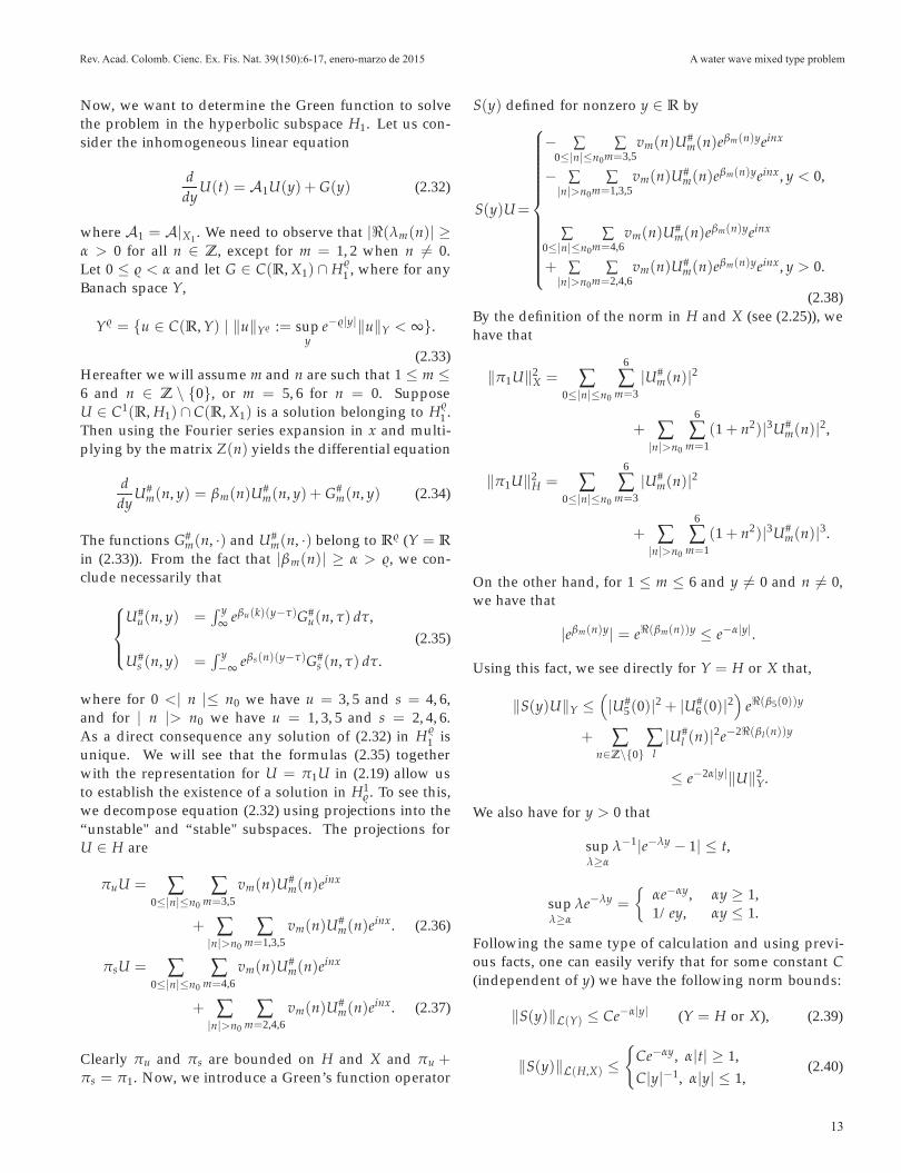
S(y) defined for nonzero y ∈ R by

S(y)U=

⎧⎪⎪⎪⎪⎪⎪⎪⎪⎪⎪⎪⎪⎨⎪⎪⎪⎪⎪⎪⎪⎪⎪⎪⎪⎪⎩

− ∑0≤|n|≤n0

∑m=3,5

vm(n)U#m(n)eβm(n)yeinx

− ∑|n|>n0

∑m=1,3,5

vm(n)U#m(n)eβm(n)yeinx, y < 0,

∑0≤|n|≤n0

∑m=4,6

vm(n)U#m(n)eβm(n)yeinx

+ ∑|n|>n0

∑m=2,4,6

vm(n)U#m(n)eβm(n)yeinx, y > 0.

(2.38)By the definition of the norm in H and X (see (2.25)), wehave that

�π1U�2X = ∑

0≤|n|≤n0

6

∑m=3

|U#m(n)|2

+ ∑|n|>n0

6

∑m=1

(1 + n2)|3U#m(n)|2,

�π1U�2H = ∑

0≤|n|≤n0

6

∑m=3

|U#m(n)|2

+ ∑|n|>n0

6

∑m=1

(1 + n2)|3U#m(n)|3.

On the other hand, for 1 ≤ m ≤ 6 and y �= 0 and n �= 0,we have that

|eβm(n)y| = e�(βm(n))y ≤ e−α|y|.

Using this fact, we see directly for Y = H or X that,

�S(y)U�Y ≤�|U#

5(0)|2 + |U#6(0)|2

�e�(β5(0))y

+ ∑n∈Z\{0}

∑l|U#

l (n)|2e−2�(βl(n))y

≤ e−2α|y|�U�2Y.

We also have for y > 0 that

supλ≥α

λ−1|e−λy − 1| ≤ t,

supλ≥α

λe−λy =

�αe−αy, αy ≥ 1,1/ey, αy ≤ 1.

Following the same type of calculation and using previ-ous facts, one can easily verify that for some constant C(independent of y) we have the following norm bounds:

�S(y)�L(Y) ≤ Ce−α|y| (Y = H or X), (2.39)

�S(y)�L(H,X) ≤�

Ce−αy, α|t| ≥ 1,C|y|−1, α|y| ≤ 1,

(2.40)

13

Quintero JR

14


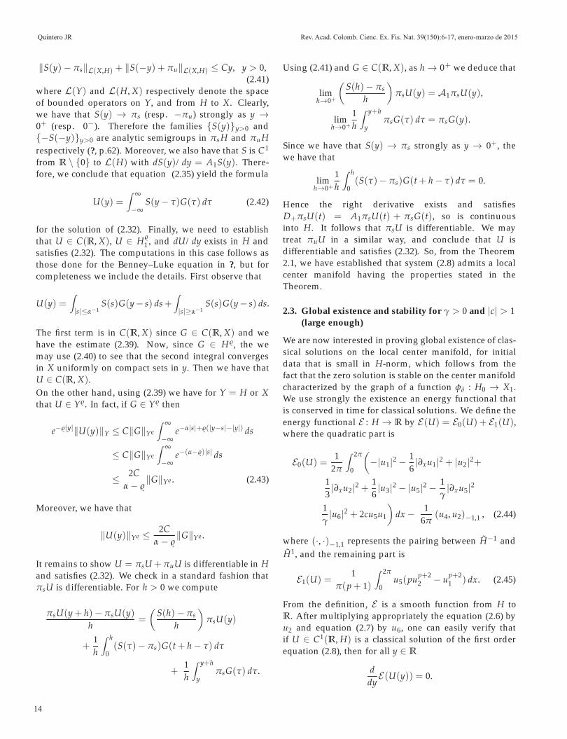
�S(y)− πs�L(X,H) + �S(−y) + πu�L(X,H) ≤ Cy, y > 0,(2.41)

where L(Y) and L(H, X) respectively denote the spaceof bounded operators on Y, and from H to X. Clearly,we have that S(y) → πs (resp. −πu) strongly as y →0+ (resp. 0−). Therefore the families {S(y)}y>0 and{−S(−y)}y>0 are analytic semigroups in πs H and πuHrespectively (?, p.62). Moreover, we also have that S is C1

from R \ {0} to L(H) with dS(y)/dy = A1S(y). There-fore, we conclude that equation (2.35) yield the formula

U(y) =∫ ∞

−∞S(y − τ)G(τ) dτ (2.42)

for the solution of (2.32). Finally, we need to establishthat U ∈ C(R, X), U ∈ H�

1 , and dU/dy exists in H andsatisfies (2.32). The computations in this case follows asthose done for the Benney–Luke equation in ?, but forcompleteness we include the details. First observe that

U(y) =∫

|s|≤α−1S(s)G(y− s) ds+

∫

|s|≥α−1S(s)G(y− s) ds.

The first term is in C(R, X) since G ∈ C(R, X) and wehave the estimate (2.39). Now, since G ∈ H�, the wemay use (2.40) to see that the second integral convergesin X uniformly on compact sets in y. Then we have thatU ∈ C(R, X).On the other hand, using (2.39) we have for Y = H or Xthat U ∈ Y�. In fact, if G ∈ Y� then

e−�|y|�U(y)�Y ≤ C�G�Y�

∫ ∞

−∞e−α|s|+�(|y−s|−|y|) ds

≤ C�G�Y�

∫ ∞

−∞e−(α−�)|s| ds

≤ 2Cα − �

�G�Y� . (2.43)

Moreover, we have that

�U(y)�Y� ≤ 2Cα − �

�G�Y� .

It remains to show U = πsU +πuU is differentiable in Hand satisfies (2.32). We check in a standard fashion thatπsU is differentiable. For h > 0 we compute

πsU(y + h)− πsU(y)h =

(S(h)− πs

h

)πsU(y)

+1h

∫ h

0(S(τ)− πs)G(t + h − τ) dτ

+1h

∫ y+h

yπsG(τ) dτ.

Using (2.41) and G ∈ C(R, X), as h → 0+ we deduce that

limh→0+

(S(h)− πs

h

)πsU(y) = A1πsU(y),

limh→0+

1h

∫ y+h

yπsG(τ) dτ = πsG(y).

Since we have that S(y) → πs strongly as y → 0+, thewe have that

limh→0+

1h

∫ h

0(S(τ)− πs)G(t + h − τ) dτ = 0.

Hence the right derivative exists and satisfiesD+πsU(t) = A1πsU(t) + πsG(t), so is continuousinto H. It follows that πsU is differentiable. We maytreat πuU in a similar way, and conclude that U isdifferentiable and satisfies (2.32). So, from the Theorem2.1, we have established that system (2.8) admits a localcenter manifold having the properties stated in theTheorem.

2.3. Global existence and stability for γ > 0 and |c| > 1(large enough)

We are now interested in proving global existence of clas-sical solutions on the local center manifold, for initialdata that is small in H-norm, which follows from thefact that the zero solution is stable on the center manifoldcharacterized by the graph of a function φδ : H0 → X1.We use strongly the existence an energy functional thatis conserved in time for classical solutions. We define theenergy functional E : H → R by E (U) = E0(U) + E1(U),where the quadratic part is

E0(U) =1

2π

∫ 2π

0

(−|u1|2 − 1

6|∂xu1|2 + |u2|2+

13|∂xu2|2 + 1

6|u3|2 − |u5|2 − 1

γ|∂xu5|2

1γ|u6|2 + 2cu5u1

)dx − 1

6π(u4, u2)−1,1 , (2.44)

where (·, ·)−1,1 represents the pairing between H−1 andH1, and the remaining part is

E1(U) =1

π(p + 1)

∫ 2π

0u5(pup+2

2 − up+21 ) dx. (2.45)

From the definition, E is a smooth function from H toR. After multiplying appropriately the equation (2.6) byu2 and equation (2.7) by u6, one can easily verify thatif U ∈ C1(R, H) is a classical solution of the first orderequation (2.8), then for all y ∈ R

ddyE (U(y)) = 0.

14


15


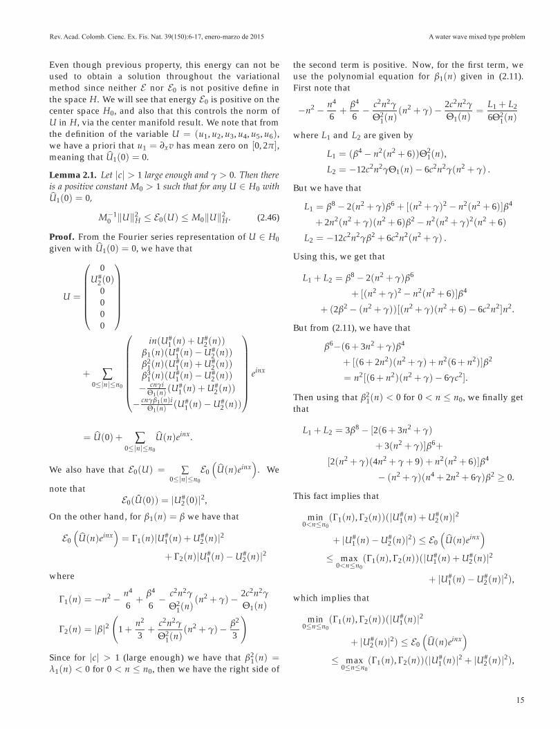
Even though previous property, this energy can not beused to obtain a solution throughout the variationalmethod since neither E nor E0 is not positive define inthe space H. We will see that energy E0 is positive on thecenter space H0, and also that this controls the norm ofU in H, via the center manifold result. We note that fromthe definition of the variable U = (u1, u2, u3, u4, u5, u6),we have a priori that u1 = ∂xv has mean zero on [0, 2π],meaning that �U1(0) = 0.

Lemma 2.1. Let |c| > 1 large enough and γ > 0. Then thereis a positive constant M0 > 1 such that for any U ∈ H0 with�U1(0) = 0,

M−10 �U�2

H ≤ E0(U) ≤ M0�U�2H. (2.46)

Proof. From the Fourier series representation of U ∈ H0given with �U1(0) = 0, we have that

U =

⎛⎜⎜⎜⎜⎜⎜⎝

0U#

2(0)0000

⎞⎟⎟⎟⎟⎟⎟⎠

+ ∑0≤|n|≤n0

⎛⎜⎜⎜⎜⎜⎜⎜⎜⎝

in(U#1(n) + U#

2(n))β1(n)(U#

1(n)− U#2(n))

β21(n)(U

#1(n) + U#

2(n))β3

1(n)(U#1(n)− U#

2(n))− cnγi

Θ1(n) (U#1(n) + U#

2(n))− cnγβ1(n)i

Θ1(n) (U#1(n)− U#

2(n))

⎞⎟⎟⎟⎟⎟⎟⎟⎟⎠

einx

= �U(0) + ∑0≤|n|≤n0

�U(n)einx.

We also have that E0(U) = ∑0≤|n|≤n0

E0

� �U(n)einx�

. We

note thatE0(U(0)) = |U#

2(0)|2,

On the other hand, for β1(n) = β we have that

E0

� �U(n)einx�= Γ1(n)|U#

1(n) + U#2(n)|2

+ Γ2(n)|U#1(n)− U#

2(n)|2

where

Γ1(n) = −n2 − n4

6+

β4

6− c2n2γ

Θ21(n)

(n2 + γ)− 2c2n2γ

Θ1(n)

Γ2(n) = |β|2�

1 +n2

3+

c2n2γ

Θ21(n)

(n2 + γ)− β2

3

�

Since for |c| > 1 (large enough) we have that β21(n) =

λ1(n) < 0 for 0 < n ≤ n0, then we have the right side of

the second term is positive. Now, for the first term, weuse the polynomial equation for β1(n) given in (2.11).First note that

−n2 − n4

6+

β4

6− c2n2γ

Θ21(n)

(n2 + γ)− 2c2n2γ

Θ1(n)=

L1 + L2

6Θ21(n)

where L1 and L2 are given by

L1 = (β4 − n2(n2 + 6))Θ21(n),

L2 = −12c2n2γΘ1(n)− 6c2n2γ(n2 + γ) .

But we have that

L1 = β8 − 2(n2 + γ)β6 + [(n2 + γ)2 − n2(n2 + 6)]β4

+ 2n2(n2 + γ)(n2 + 6)β2 − n2(n2 + γ)2(n2 + 6)

L2 = −12c2n2γβ2 + 6c2n2(n2 + γ) .

Using this, we get that

L1 + L2 = β8 − 2(n2 + γ)β6

+ [(n2 + γ)2 − n2(n2 + 6)]β4

+ (2β2 − (n2 + γ))[(n2 + γ)(n2 + 6)− 6c2n2]n2.

But from (2.11), we have that

β6−(6 + 3n2 + γ)β4

+ [(6+ 2n2)(n2 + γ) + n2(6+ n2)]β2

= n2[(6+ n2)(n2 + γ)− 6γc2].

Then using that β21(n) < 0 for 0 < n ≤ n0, we finally get

that

L1 + L2 = 3β8 − [2(6+ 3n2 + γ)

+ 3(n2 + γ)]β6+

[2(n2 + γ)(4n2 + γ + 9) + n2(n2 + 6)]β4

− (n2 + γ)(n4 + 2n2 + 6γ)β2 ≥ 0.

This fact implies that

min0<n≤n0

(Γ1(n), Γ2(n))(|U#1(n) + U#

2(n)|2

+ |U#1(n)− U#

2(n)|2) ≤ E0

� �U(n)einx�

≤ max0<n≤n0

(Γ1(n), Γ2(n))(|U#1(n) + U#

2(n)|2

+ |U#1(n)− U#

2(n)|2),which implies that

min0≤n≤n0

(Γ1(n), Γ2(n))(|U#1(n)|2

+ |U#2(n)|2) ≤ E0

� �U(n)einx�

≤ max0≤n≤n0

(Γ1(n), Γ2(n))(|U#1(n)|2 + |U#

2(n)|2),

15

Quintero JR

16


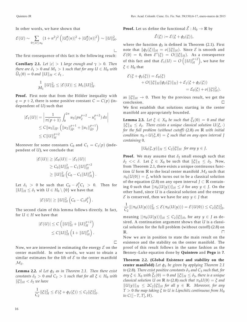
In other words, we have shown that

E (U) ∼ ∑0≤n≤n0

(1 + n2)2(|U#

1(n)|2 + |U#2(n)|2

)∼ �U�2

H .

The first consequence of this fact is the following result:

Corollary 2.1. Let |c| > 1 large enough and γ > 0. Thenthere are δ1 > 0 and M1 > 1 such that for any U ∈ H0 withU1(0) = 0 and �U�H < δ1 ,

1M1

�U�2H ≤ |E (U)| ≤ M1�U�2

H.

Proof. First note that from the Hölder inequality withq = p + 2, there is some positive constant C = C(p) (in-dependent of U) such that

|E1(U)| =∣∣∣∣

1π(p + 1)

∫ 2π

0u5(pup+2

2 − up+21 ) dx

∣∣∣∣≤ C�u5�H1

(�u2�p+1

H1 + �u1�p+1H1

)

≤ C�U�p+2H

Moreover for some constants C0 and C1 = C1(p) (inde-pendent of U), we conclude that

|E (U)| ≥ |E0(U)| − |E1(U)|≥ C0�U�2

H − C1�U�p+2H

≥ �U�2H

(C0 − C1�U�p

H

).

Let δ1 > 0 be such that C0 − δp1 C1 > 0. Then for

�U�H ≤ δ1 with U ∈ H0 \ {0} we have that

|E (U)| ≥ �U�2H

(C0 − C1δ

p1

).

The second claim of this lemma follows directly. In fact,for U ∈ H we have that

|E (U)| ≤ C(�U�2

H + �U�p+2H

)

≤ C�U�2H

(1 + �U�p

H

).

Now, we are interested in estimating the energy E on thecenter manifold. In other words, we want to obtain asimilar estimates for the lift of E to the center manifoldMδ.

Lemma 2.2. sl Let φδ as in Theorem 2.1. Then there existconstants δ2 > 0 and C2 > 1 such that for all ξ ∈ H0 with�ξ�H < δ2 we have

1C2

�ξ�2H ≤ E (ξ + φδ(ξ)) ≤ C2�ξ�2

H .

Proof. Let us define the functional E : H0 → R by

E(ξ) := E (ξ + φδ(ξ)),

where the function φδ is defined in Theorem (2.1). Firstnote that �φδ(ξ)�H = o(�ξ�H). Since E is smooth andE (0) = 0, then E �(ξ) = O(�ξ�H). As a consequence

of this fact and that E1(U) = O(�U�p+2

H

), we have for

ξ ∈ H0 that

E (ξ + φδ(ξ)) = E0(ξ)

+ O(�ξ�H�φδ(ξ)�H) + E1(ξ + φδ(ξ))

= E0(ξ) + o(�ξ�2H).

as �ξ�H → 0. Then by the previous result, we get theconclusion.We first establish that solutions starting in the centermanifold are appropriately bounded.

Lemma 2.3. Let ξ ∈ X0 be such that ξ1(0) = 0 and that�ξ�X ≤ δ2. There exists a unique classical solution U(ξ, ·)for the full problem (without cutoff) (2.8) on R with initialcondition π0 ◦ U(ξ, 0) = ξ such that on any open interval Jcontaining 0,

�U0(ξ, y)�H ≤ C2�ξ�H for any y ∈ J.

Proof. We may assume that δ2 small enough such thatδ2 << δ. Let ξ ∈ X0 be such that �ξ�X ≤ δ2. Now,from Theorem 2.1, there exists a unique continuous func-tion U form R to the local center manifold Mδ such thatπ0(U(0)) = ξ, which turns out to be a classical solutionof the equation (2.8) on any open interval J ⊂ R contain-ing 0 such that �π0(U(y))�H ≤ δ for any y ∈ J. On theother hand, since U is a classical solution and the energyE is conserved, then we have for any y ∈ J that

1C2

�|π0(U(y))�2H ≤ E (π0(U(y))) = E (U(0)) ≤ C2�ξ�2

H ,

meaning ||π0(U(y))�H ≤ C2�ξ�H , for any y ∈ J as de-sired. A continuation argument shows that U is a classi-cal solution for the full problem (without cutoff) (2.8) onR.Now we are in position to state the main result on theexistence and the stability on the center manifold. Theproof of this result follows in the same fashion as theBenney–Luke equation done by Quintero and Pego in ?.

Theorem 2.2. (Global Existence and stability on thecenter manifold) Let φδ be given by applying Theorem 2.1to (2.8). There exist positive constants δ3 and C3 such that, forany ξ ∈ X0 with ξ1(0) = 0 and �ξ�H ≤ δ3, there is a uniqueclassical solution U on R to (2.8) such that π0U(0) = ξ and�U(y)�H ≤ 2C2�ξ�H for all y ∈ R. Moreover, for anyT > 0 the map taking ξ to U is Lipschitz continuous from H0to C([−T, T], H).

16


17


Acknowledgments. J. R. Quintero was supported bythe Mathematics Department at Universidad del Valle(Colombia) under the project C.I. 7910.

References

Grover, M. (2001). An existence theory for three-dimensionalperiodic travelling gravity-capillary water waves withbounded transverse profiles. Physica D 152(1): 295–415.

Grover, M., Mielke, A. (2001). A spatial dynamics approachto three-dimensional gravity-capillary steady water waves.Proc. Royal Soc. Edin. A131(1): 83–136.

Grover, M., Schneider, A. (2001). Modulating pulse solutionsfor a class of nonlinear wave equations. Commun. Math. Phys.219: 489–522.

Haragus–Courcelle M., Schneider G. (1999). Bifurcating frontsfor the Taylor-Couette problem in infinite cylinders. Z.Angew. Math. Phys. 50: 120–151.

Kirchgässner, A. (1982). Wave solutions of reversible systemsand applications. J. Diff. Eqns. 45: 113–127.

Mielke, A. (1988). Reduction of quasilinear elliptic equationsin cylindrical domains with applications. Math. Meth. Appli.Sci. 101: 51–56.

Mielke, A. (1991). Hamiltonian and Lagrangian Flows on CenterManifolds. Berlin: Springer–Verlag.

Mielke, A. (1992). On nonlinear problems of mixed type: aqualitative theory using infinite-dimensional center mani-folds. J. Dyn. Diff. Eqns. 4 (1): 419–443.

Pazy, A. (1983). Semigroups of Linear Operators and Applicationsto Partial Differential Equations. Springer–Verlag, New York.

Quintero J., Pego R. (1999). Two–dimensional solitary wavesfor a Benney–Luke equation. Physica D 132: 476–496.

Quintero J., Pego R. (2002). A host of Travelling Waves in aModel of Three-Dimensional Water-Wave Dynamics. Non-linear Science 12: 59–83.

Sandstede B., Scheel A. (1999). An Essential instability ofpulses and bifurcations to modulated travelling waves. Proc.Roy. Soc. Edin. A 129: 1263–1290.

Sandstede B., Scheel A. (2004). Defects in oscillatory media:Toward a classification. SIAM J. Appl. Dynam. Syst. 3: 1–68.

Scarpellini, B. (1990). On nonlinear problems of mixed type:a qualitative theory using infinite-dimensional center mani-fold. I and II. J. Appl. Math. Phys. (ZAMP). 42: 289–314.

Vanderbauwhede, A., and Iooss, G. (1982). On nonlinearproblems of mixed type: a qualitative theory using infinite-dimensional center manifold. I and II. Dynamics Reported,New Series 1: 125–163.

Vanderbauwhede A. (1989). Centre manifolds, normal formsand elementary bifurcations. Dynamics Reported, New Series2: 89-169.

17

Documents

A water wave mixed type problem: existence of periodic ... · En este artículo establecemos un resultado de existencia de ondas periódicas para un sistema 2D del tipo Boussinesq