1

1

A Walk through"Bildverarbeitung WS 2007/08"

2

Definition of Image Understanding

Image understanding is the task-oriented reconstruction andinterpretation of a scene by means of images

Image understanding is the task-oriented reconstruction andinterpretation of a scene by means of images

scene: section of the real worldstationary (3D) or moving (4D)

image: view of a sceneprojection, density image (2D)depth image (2 1/2D)image sequence (3D)

reconstruction computer-internal scene descriptionand interpretation: quantitative + qualitative + symbolic

task-oriented: for a purpose, to fulfill a particular taskcontext-dependent, supporting actions of an agent

2

3

Technical Colour ModelsRGB colour model

R

G

B

magentacyan

yellowTypical discretization:8 bits per colour dimension=> 16,77,216 colours

CMY colour model

C 1 RM = 1 - GY 1 B

HSI colour model

Hue:

H = Θ if B ≤ G360 - Θ if B > G

1/2 [(R-G) + (R-B)]Θ = cos-1

[(R-G)2 + (R-B)(G-B)]1/2

Saturation: 3

S = 1 - [min (R, G, B)](R + G + B)

Intensity:I = 1/3 (R + G + B)

4

Sampling Theorem

Shannon´s Sampling Theorem:

A bandlimited function with bandwidth W can be exactlyreconstructed from equally spaced samples, if the samplingdistance is not larger than 1

2W

bandwidth = largest frequency contained in signal(=> Fourier decomposition of a signal)

Analogous theorem holds for 2D signals with limited spatialfrequencies Wx and Wy

3

5

Perspective Projection Geometry

Projective geometry relates the coordinates of a point in a scene to thecoordinates of its projection onto an image plane.Perspective projection is an adequate model for most cameras.

•

••

xy

xpyp

zp = f

v = xyz

image plane

optical center

x f zxp =

y f zyp=

scene pointimage point

Projection equations:

focal distance f

z = optical axis

Vp = xpypzp

6

Connectivity in Digital Images

Connectivity is an important property of subsets of pixels. It is basedon adjacency (or neighbourhood):

Pixels are 4-neighboursif their distance is D4 = 1

Pixels are 8-neighboursif their distance is D8 = 1

A path from pixel P to pixel Q is a sequence of pixels beginning atQ and ending at P, where consecutive pixels are neighbours.In a set of pixels, two pixels P and Q are connected, if there is apath between P and Q with pixels belonging to the set.A region is a set of pixels where each pair of pixels is connected.

all 4-neighbours ofcenter pixel

all 8-neighbours ofcenter pixel

4

7

Principle of Greyvalue Interpolation

• •• •

• •

••

•••

•

••• •Greyvalue interpolation = computation of

unknown greyvalues at locations (u´v´) fromknown greyvalues at locations (x´y´)

Two ways of viewing interpolation in the context of geometrictransformations:

A Greyvalues at grid locations (x y) in old image are placed atcorresponding locations (x´y´) in new image: g(x´y´) = g(T(x y))=> interpolation in new image

B Grid locations (u´v´) in new image are transformed intocorresponding locations (u v) in old image: g(u v) = g(T-1(u´v´))=> interpolation in old image

We will take view B:Compute greyvalues between grid from greyvalues at grid locations.

8

Global Image Properties

Global image properties refer to an image as a whole rather thancomponents. Computation of global image properties is often requiredfor image enhancement, preceding image analysis.We treat

• empirical mean and variance• histograms• projections• cross-sections• frequency spectrum

5

9

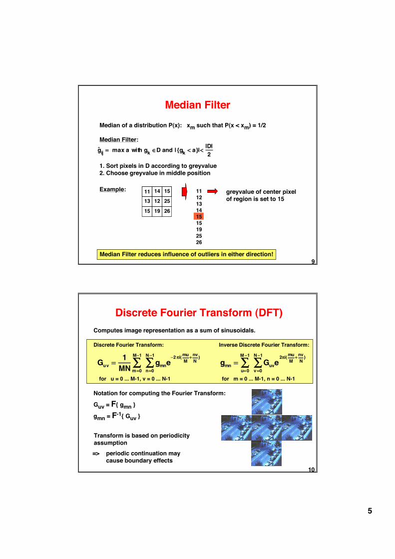
Median FilterMedian of a distribution P(x): xm such that P(x < xm) = 1/2

Median Filter:ˆ g ij = max a with gk ∈D and | {gk < a}|< |D|

2

1. Sort pixels in D according to greyvalue2. Choose greyvalue in middle position

Example: 11 14 15

13 12 25

15 19 26

111213141515192526

greyvalue of center pixelof region is set to 15

Median Filter reduces influence of outliers in either direction!

10

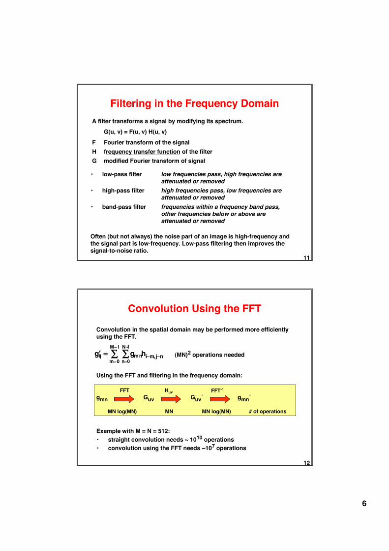
Discrete Fourier Transform (DFT)

Guv =1

MN gmn

n=0

N−1

∑m=0

M−1

∑ e−2πi( mu

M+nv

N)

gmn = Guvv=0

N−1

∑u=0

M −1

∑ e2πi( mu

M+nv

N)

Transform is based on periodicityassumption

Discrete Fourier Transform: Inverse Discrete Fourier Transform:

=> periodic continuation maycause boundary effects

for u = 0 ... M-1, v = 0 ... N-1 for m = 0 ... M-1, n = 0 ... N-1

Notation for computing the Fourier Transform:

Guv = F{ gmn }

gmn = F-1{ Guv }

Computes image representation as a sum of sinusoidals.

6

11

Filtering in the Frequency DomainA filter transforms a signal by modifying its spectrum.

G(u, v) = F(u, v) H(u, v)F Fourier transform of the signalH frequency transfer function of the filterG modified Fourier transform of signal

• low-pass filter low frequencies pass, high frequencies areattenuated or removed

• high-pass filter high frequencies pass, low frequencies areattenuated or removed

• band-pass filter frequencies within a frequency band pass,other frequencies below or above are attenuated or removed

Often (but not always) the noise part of an image is high-frequency andthe signal part is low-frequency. Low-pass filtering then improves thesignal-to-noise ratio.

12

Convolution Using the FFT

Convolution in the spatial domain may be performed more efficientlyusing the FFT.

′ g ij = gmnn=0

N -1∑

m= 0

M−1∑ hi−m,j−n (MN)2 operations needed

Using the FFT and filtering in the frequency domain:

gmn Guv Guv´ gmn´FFT Huv FFT-1

MN log(MN) MN MN log(MN) # of operations

Example with M = N = 512:• straight convolution needs ~ 1010 operations• convolution using the FFT needs ~107 operations

7

13

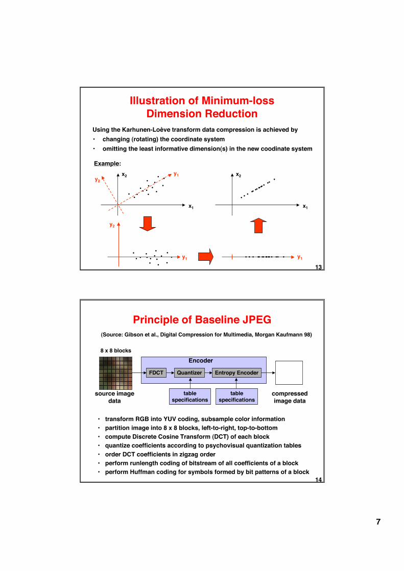
Illustration of Minimum-lossDimension Reduction

Using the Karhunen-Loève transform data compression is achieved by• changing (rotating) the coordinate system• omitting the least informative dimension(s) in the new coodinate system

Example:

x1

x2

• •••

• • •• •

•••

•

••

x1

x2

• • • •• •••••• •• •

•

y1y2

• •••• •

•

••

•• • •• • y1

y2

• • • •• ••••• • •• •• y1

14

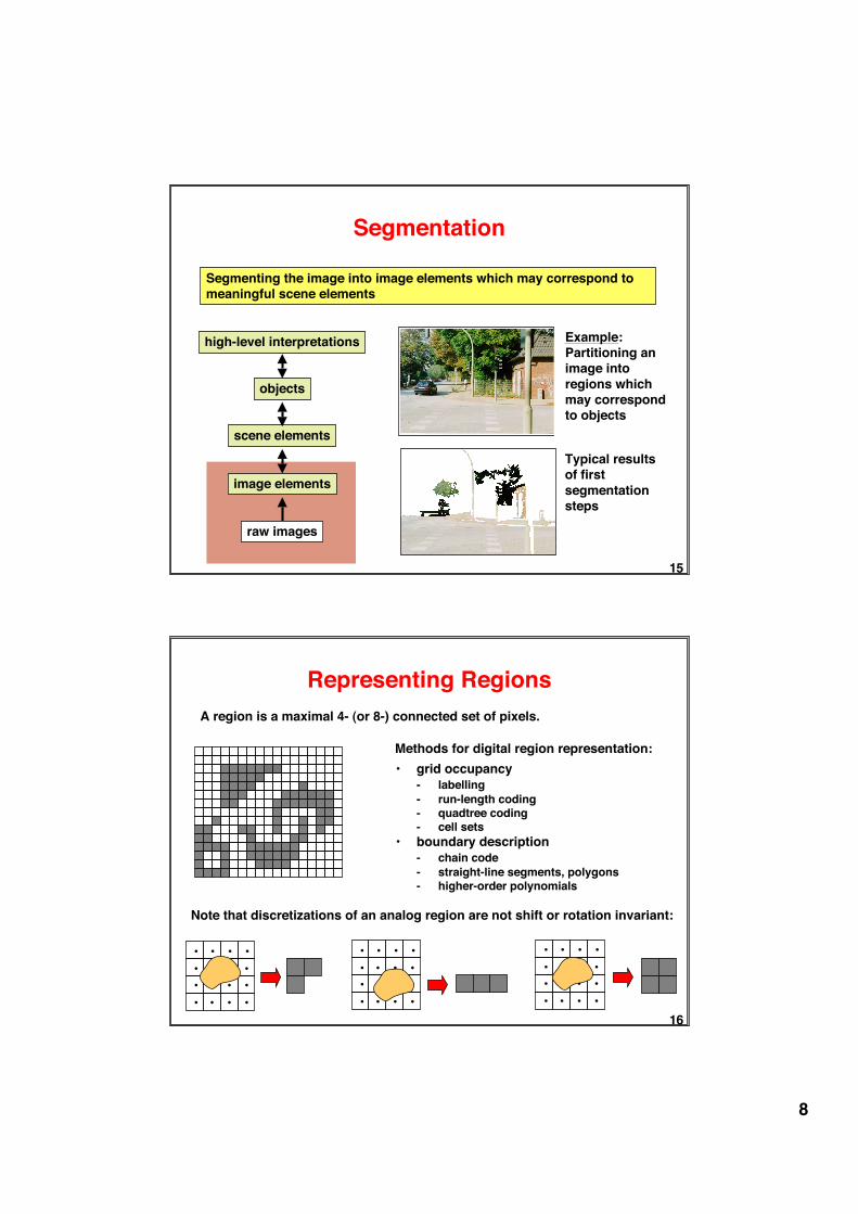
Principle of Baseline JPEG

FDCT Quantizer Entropy Encoder

Encoder

tablespecifications

tablespecifications

8 x 8 blocks

source imagedata

compressedimage data

(Source: Gibson et al., Digital Compression for Multimedia, Morgan Kaufmann 98)

• transform RGB into YUV coding, subsample color information• partition image into 8 x 8 blocks, left-to-right, top-to-bottom• compute Discrete Cosine Transform (DCT) of each block• quantize coefficients according to psychovisual quantization tables• order DCT coefficients in zigzag order• perform runlength coding of bitstream of all coefficients of a block• perform Huffman coding for symbols formed by bit patterns of a block

8

15

Segmentation

Segmenting the image into image elements which may correspond tomeaningful scene elements

high-level interpretations

objects

scene elements

image elements

raw images

Typical resultsof firstsegmentationsteps

Example:Partitioning animage intoregions whichmay correspondto objects

16

Representing RegionsA region is a maximal 4- (or 8-) connected set of pixels.

Methods for digital region representation:• grid occupancy

- labelling- run-length coding- quadtree coding- cell sets

• boundary description- chain code- straight-line segments, polygons- higher-order polynomials

Note that discretizations of an analog region are not shift or rotation invariant:

• • • •• • • •• • • •• • • •

• • • •• • • •• • • •• • • •

• • • •• • • •• • • •• • • •

9

17

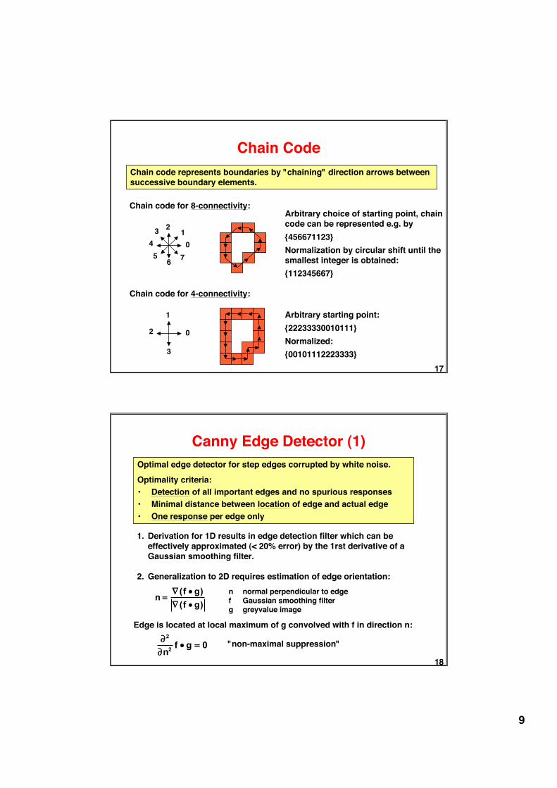
Chain CodeChain code represents boundaries by "chaining" direction arrows betweensuccessive boundary elements.

01

2345

6 7

Arbitrary choice of starting point, chaincode can be represented e.g. by{456671123}Normalization by circular shift until thesmallest integer is obtained:{112345667}

Chain code for 8-connectivity:

0

1

2

3

Chain code for 4-connectivity:

Arbitrary starting point:{22233330010111}Normalized:{00101112223333}

18

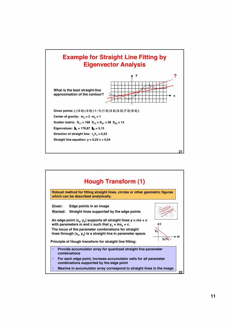
Canny Edge Detector (1)Optimal edge detector for step edges corrupted by white noise.Optimality criteria:• Detection of all important edges and no spurious responses• Minimal distance between location of edge and actual edge• One response per edge only

1. Derivation for 1D results in edge detection filter which can beeffectively approximated (< 20% error) by the 1rst derivative of aGaussian smoothing filter.

2. Generalization to 2D requires estimation of edge orientation:

n =

∇ (f • g)∇ (f • g)

n normal perpendicular to edgef Gaussian smoothing filterg greyvalue image

Edge is located at local maximum of g convolved with f in direction n:

∂2

∂n2 f • g = 0 "non-maximal suppression"

10

19

Canny Edge Detector (2)Algorithm includes- choice of scale σ- hysteresis thresholding to avoid streaking (breaking up edges)- "feature synthesis" by selecting large-scale edges dependent on

lower-scale support

1. Convolve image g with Gaussian filter f of scale σ 2. Estimate local edge normal direction n for each point in the image3. Find edge locations using non-maximal suppression4. Compute magnitude of edges by5. Threshold edges with hysteresis to eliminate spurious edges6. Repeat steps (1) through (5) for increasing values of σ 7. Aggregate edges at multiple scales using feature synthesis

∇ (f • g)

20

GroupingTo make sense of image elements, they first have to be grouped intolarger structures.

Example: Grouping noisy edge elements into a straight edge

Important methods:• Fitting• Clustering• Hough Transform• Relaxation

Essential problem:Obtaining globally valid results bylocal decisions

- locally compatible- globally incompatible

11

21

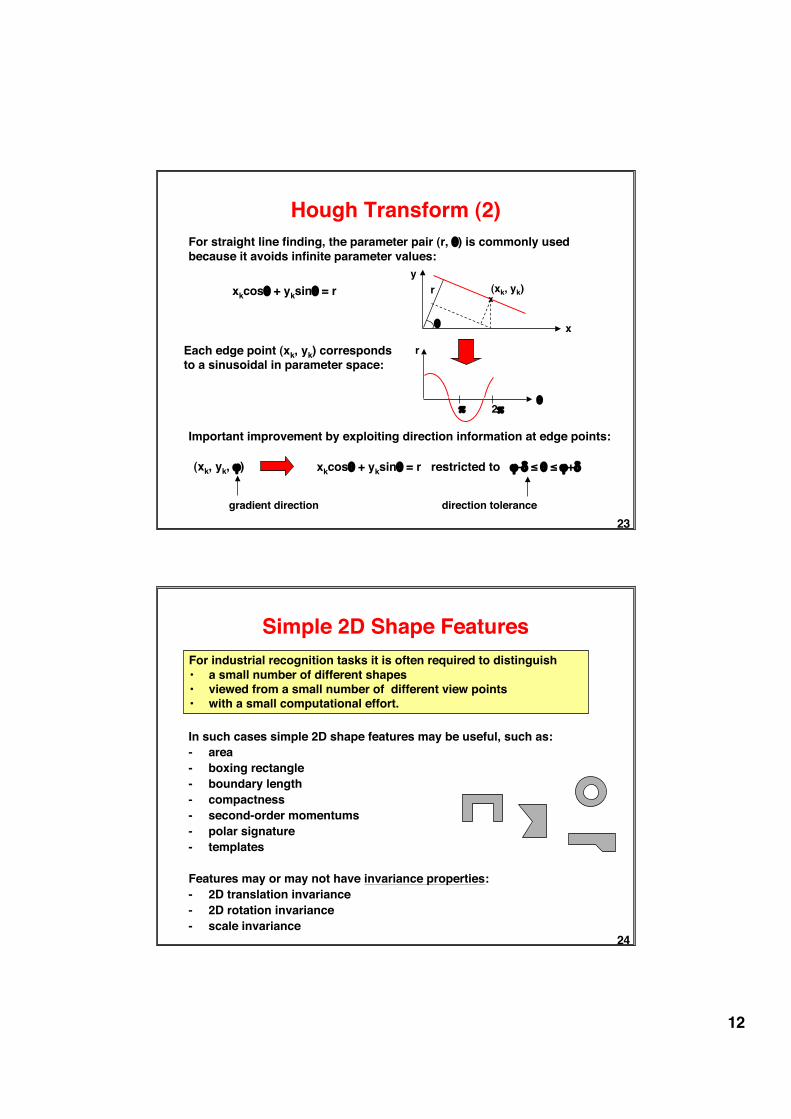
Example for Straight Line Fitting byEigenvector Analysis

••

••

•• •

• x

y

What is the best straight-lineapproximation of the contour?

Given points: { (-5 0) (-3 0) (-1 -1) (1 0) (3 2) (5 3) (7 2) (9 2) }

Scatter matrix: S11 = 168 S12 = S21 = 38 S22 = 14

Eigenvalues: λ1 = 176,87 λ2 = 5,13

Straight line equation: y = 0,23 x + 0,54

?

Center of gravity: mx = 2 my = 1

•

Direction of straight line: ry/rx = 0,23

22

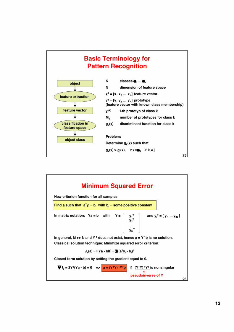
Hough Transform (1)Robust method for fitting straight lines, circles or other geometric figureswhich can be described analytically.

Given: Edge points in an imageWanted: Straight lines supported by the edge points

An edge point (xk, yk) supports all straight lines y = mx + cwith parameters m and c such that yk = mxk + c.The locus of the parameter combinations for straightlines through (xk, yk) is a straight line in parameter space.

m

c

yk/xk

yk

• Provide accumulator array for quantized straight line parametercombinations

• For each edge point, increase accumulator cells for all parametercombinations supported by the edge point

• Maxima in accumulator array correspond to straight lines in the image

Principle of Hough transform for straight line fitting:

12

23

Hough Transform (2)For straight line finding, the parameter pair (r, θ) is commonly usedbecause it avoids infinite parameter values:

xkcosθ + yksinθ = rx

r

θ

(xk, yk)

x

y

Each edge point (xk, yk) correspondsto a sinusoidal in parameter space:

π 2πθ

r

Important improvement by exploiting direction information at edge points:

(xk, yk, ϕ) xkcosθ + yksinθ = r restricted to ϕ-δ ≤ θ ≤ ϕ+δ

direction tolerancegradient direction

24

Simple 2D Shape FeaturesFor industrial recognition tasks it is often required to distinguish• a small number of different shapes• viewed from a small number of different view points• with a small computational effort.

In such cases simple 2D shape features may be useful, such as:- area- boxing rectangle- boundary length- compactness- second-order momentums- polar signature- templates

Features may or may not have invariance properties:- 2D translation invariance- 2D rotation invariance- scale invariance

13

25

Basic Terminology forPattern Recognition

feature extraction

feature vector

object

classification infeature space

object class

K classes ω1 ... ωK

N dimension of feature spacexT = [x1 x2 ... xN] feature vectoryT = [y1 y2 ... yN] prototype(feature vector with known class membership)yi

(k) i-th prototyp of class kMk number of prototypes for class kgk(x) discriminant function for class k

Problem:Determine gk(x) such that

gk(x) > gj(x), ∀ x eωK ∀ k ≠ j

26

Minimum Squared ErrorNew criterion function for all samples:

Find a such that aTyi = bi with bi = some positive constant

In matrix notation: Ya = b with Y = y1T

y2T

...

yMT

and yiT = [ yi1 ... yiN ]

In general, M >> N and Y-1 does not exist, hence a = Y-1b is no solution.Classical solution technique: Minimize squared error criterion:

Js(a) = ||Ya - b||2 = Σ (aTyi - bi)2

Closed-form solution by setting the gradient equal to 0.

„Js = 2YT(Ya - b) = 0 => a = (YTY)-1YTb if (YTY)-1YT is nonsingular

pseudoinverse of Y

�

∇

14

27

Statistical Decision Theory

Generating decision functions from a statistical characterization of classes(as opposed to a characterization by prototypes)

Advantages:1. The classification scheme may be designed to satisfy an objective

optimality criterion:Optimal decisions minimize the probability of error.

2. Statistical descriptions may be much more compact than a collectionof prototypes.

3. Some phenomena may only be adequately described using statistics,e.g. noise.

28

General Framework forBayes Classification

Statistical decision theory which minimizes the probability of error forclassifications based on uncertain evidence

ω1 ... ωK K classesP(ωk) prior probability that an object of class k will be observedx = [x1 ... xN] N-dimensional feature vector of an objectp(x|ωk) conditional probability ("likelihood") of observing x given

that the object belongs to class ωK

P(ωk|x) conditional probability ("posterior probability") that an object belongs to class ωK given x is observed

Bayes decision rule:Classify given evidence x as class ω´ such that ω´ minimizes theprobability of error P(ω ≠ ω´| x) => Choose ω´ which maximizes the posterior probability P(ω | x)gi(x) = P(ωi|x) are discriminant functions.

15

29

Motion Analysis

Motion detectionRegister locations in an image sequence which have change due to motionMoving object detection and trackingDetect individual moving objects, determine and predict object trajectories,track objects with a moving cameraDerivation of 3D object propertiesDetermine 3D object shape from multiple views ("shape from motion")

Motion analysis of digital images is based on a temporal sequence ofimage frames of a coherent scene."sparse sequence" => few frames, temporally spaced apart,

considerable differences between frames"dense sequence" => many frames, incremental time steps,

incremental differences between framesvideo => 50 half frames per sec, interleaving,

line-by-line sampling

30

Kalman Filters (1)A Kalman filter provides an iterative scheme for (i) predicting an event and(ii) incorporating new measurements.

prediction measurement

Assume a linear system with observations depending linearly on thesystem state, and white Gaussian noise disturbing the system evolutionand the observations:

xk+1 = Akxk + wkzk = Hkxk + vk

xk quantity of interest ("state") at time kAk model for evolution of xkwk zero mean Gaussian noise with

covariance Qkzk observations at time kHk relation of observations to statevk zero mean Gaussian noise with

covariance RkOften, Ak, Qk, Hk and Rk are constant.

What is the best estimate of xkbased on the previous estimatexk-1 and the observation zk?

16

31

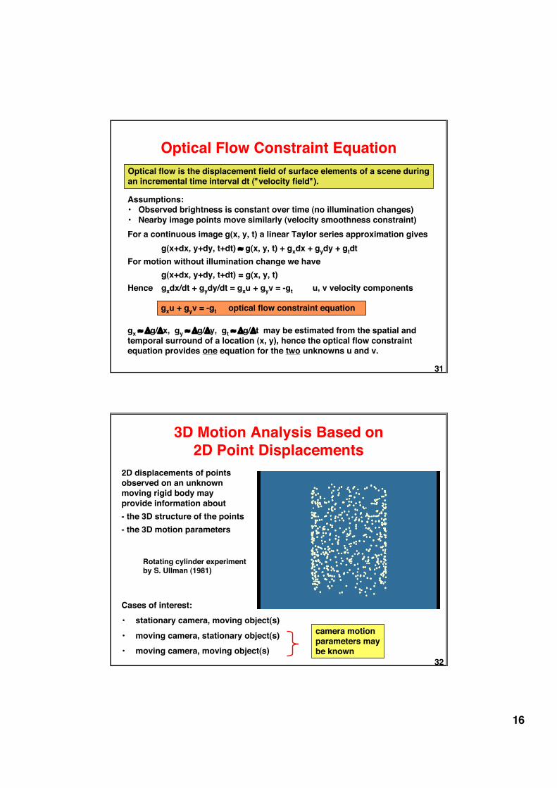
Optical Flow Constraint EquationOptical flow is the displacement field of surface elements of a scene duringan incremental time interval dt ("velocity field").

Assumptions:• Observed brightness is constant over time (no illumination changes)• Nearby image points move similarly (velocity smoothness constraint) For a continuous image g(x, y, t) a linear Taylor series approximation gives

g(x+dx, y+dy, t+dt) ≈ g(x, y, t) + gxdx + gydy + gtdtFor motion without illumination change we have

g(x+dx, y+dy, t+dt) = g(x, y, t)Hence gxdx/dt + gydy/dt = gxu + gyv = -gt u, v velocity components

gxu + gyv = -gt optical flow constraint equation

gx ≈ Δg/Δx, gy ≈ Δg/Δy, gt ≈ Δg/Δt may be estimated from the spatial andtemporal surround of a location (x, y), hence the optical flow constraintequation provides one equation for the two unknowns u and v.

32

3D Motion Analysis Based on2D Point Displacements

2D displacements of pointsobserved on an unknownmoving rigid body mayprovide information about- the 3D structure of the points- the 3D motion parameters

Cases of interest:• stationary camera, moving object(s)• moving camera, stationary object(s)• moving camera, moving object(s)

camera motionparameters maybe known

Rotating cylinder experimentby S. Ullman (1981)

17

33

Essential MatrixGeometrical constraints derived from 2 views of a point in motion

z

x

y

• vm • vm+1Rmtm

•

• motion between image m and m+1may be decomposed into1) rotation Rm about origin ofcoordinate system (= optical center)2) translation tm

• observations are given by directionvectors nm and nm+1 along projectionrays

Rmnm, tm and nm are coplanar: [tm x Rmnm]T nm+1 = 0

After some manipulation: nmT Em nm+1 = 0 E = essential matrix

with Em = and Rm =

nm

nm+1

tmxr1 tmxr2 tmxr3

|

|

|

|

|

|r1 r2 r3

|

|

|

|

|

|

34

Principle of Shape from Shading

Physical surface properties, surface orientation, illumination and viewingdirection determine the greyvalue of a surface patch in a sensor signal.For a single object surface viewed in one image, greyvalue changes aremainly caused by surface orientation changes.The reconstruction of arbitrary surface shapes is not possible becausedifferent surface orientations may give rise to identical greyvalues.Surface shapes may be uniquely reconstructed from shading information ifpossible surface shapes are constrained by smoothness assumptions.

See "Shape from Shading" (B.K.P. Horn, M.J. Brooks, eds.), MIT Press 1989

a: patch with known orientationb, c: neighbouring patches with similar orientationsb´: radical different orientation may not be

neighbour of a

Principle of incremental procedure for surface shape reconstruction:

ab

cb´

18

35

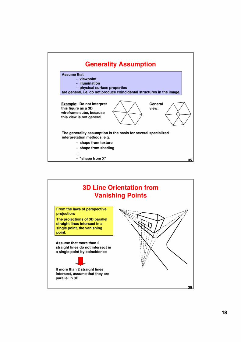
Generality AssumptionAssume that

- viewpoint- illumination- physical surface properties

are general, i.e. do not produce coincidental structures in the image.

Example: Do not interpretthis figure as a 3Dwireframe cube, becausethis view is not general.

Generalview:

The generality assumption is the basis for several specializedinterpretation methods, e.g.

- shape from texture- shape from shading...- "shape from X"

36

3D Line Orientation fromVanishing Points

From the laws of perspectiveprojection:The projections of 3D parallelstraight lines intersect in asingle point, the vanishingpoint.

Assume that more than 2straight lines do not intersect ina single point by coincidence

If more than 2 straight linesintersect, assume that they areparallel in 3D

19

37

Object Recognition byRelational Matching

Principle:• construct relational model(s) for object class(es)• construct relational image description• compute R-morphism (best partial match) between image and

model(s)• top-down verification with extended model

AB

CD

E

FG

r1r2

r1

r1

r3

r3

r2

r4

r1r2

r4

a

b

c

d e

f

g

h

i

jr1

r2r3

r1

r2

r3

r1

r4

r4

r1

r2r2

r2r3

r3

r1r1

r1model image

38

Partonomy of Object Parts

shaft dimensioning

cylinder dimensioning arrow

symmetry line

closed contour

auxiliarydimensioning line

double arrow

line arrow text

graphic primitives

20

39

SIFT Features Summary

• SIFT features are reasonably invariant to rotation, scaling, andillumination changes.

• They can be used for matching and object recognition (among otherthings).

• Robust to occlusion: as long as we can see at least 3 features fromthe object we can compute the location and pose.

• Efficient on-line matching: recognition can be performed in close-to-real time (at least for small object databases).

40

Implicit Shape Model - Recognition (2)Interest Points Matched Codebook Entries Probabilistic Voting

Voting Space(continuous)

Backprojectionof Maxima

BackprojectedHypotheses

Refined Hypotheses(uniform sampling)

Segmentation

• Spatial feature configurations• Interleaved object recognition

and segmentation

21

41

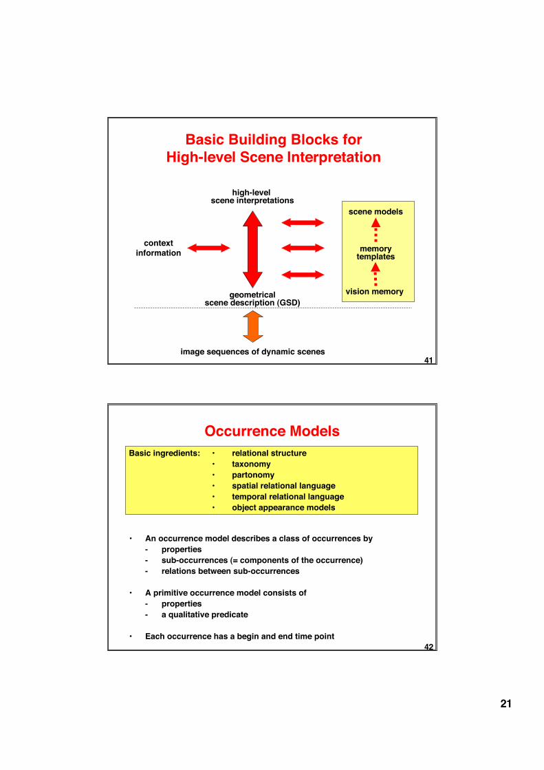
Basic Building Blocks forHigh-level Scene Interpretation

geometricalscene description (GSD)

image sequences of dynamic scenes

high-level scene interpretations

scene models

vision memory

memorytemplates

contextinformation

42

Occurrence Models

• An occurrence model describes a class of occurrences by- properties- sub-occurrences (= components of the occurrence)- relations between sub-occurrences

• A primitive occurrence model consists of- properties- a qualitative predicate

• Each occurrence has a begin and end time point

Basic ingredients: • relational structure• taxonomy• partonomy• spatial relational language• temporal relational language• object appearance models

22

43

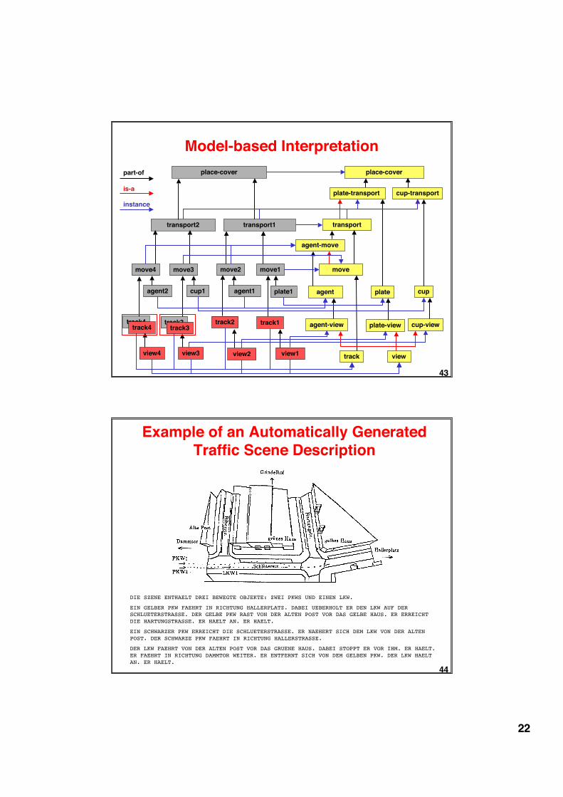
Model-based Interpretationplace-cover

plate

move

plate-transport

transport

plate-view

agent cup

cup-view

cup-transport

agent-view

agent-move

move1move2

place-cover

transport2 transport1

plate1agent1

viewtrack

track2 track1

view2 view1

move3move4

cup1

track3track4

agent2

view3view4

track4 track3

part-of

is-a

instance

44

Example of an Automatically GeneratedTraffic Scene Description

DIE SZENE ENTHAELT DREI BEWEGTE OBJEKTE: ZWEI PKWS UND EINEN LKW.

EIN GELBER PKW FAEHRT IN RICHTUNG HALLERPLATZ. DABEI UEBERHOLT ER DEN LKW AUF DERSCHLUETERSTRASSE. DER GELBE PKW RAST VON DER ALTEN POST VOR DAS GELBE HAUS. ER ERREICHTDIE HARTUNGSTRASSE. ER HAELT AN. ER HAELT.

EIN SCHWARZER PKW ERREICHT DIE SCHLUETERSTRASSE. ER NAEHERT SICH DEM LKW VON DER ALTENPOST. DER SCHWARZE PKW FAEHRT IN RICHTUNG HALLERSTRASSE.

DER LKW FAEHRT VON DER ALTEN POST VOR DAS GRUENE HAUS. DABEI STOPPT ER VOR IHM. ER HAELT.ER FAEHRT IN RICHTUNG DAMMTOR WEITER. ER ENTFERNT SICH VON DEM GELBEN PKW. DER LKW HAELTAN. ER HAELT.

23

45

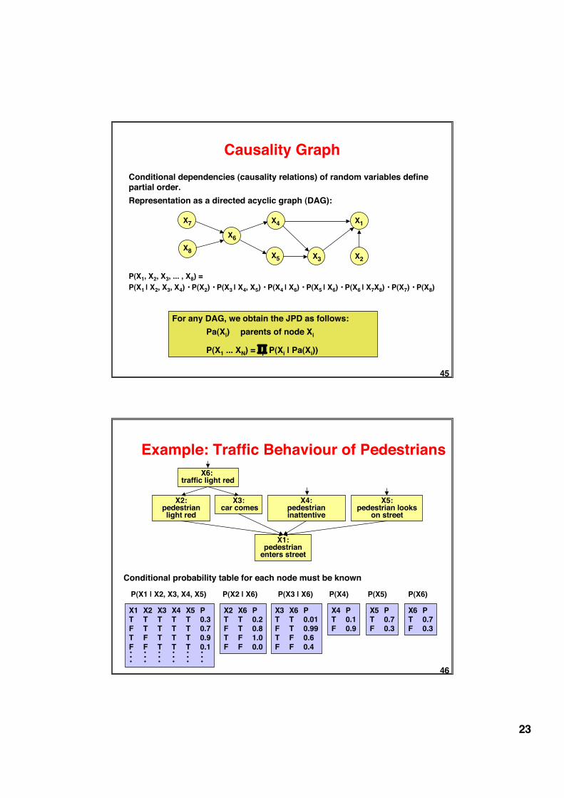
Causality GraphConditional dependencies (causality relations) of random variables definepartial order.Representation as a directed acyclic graph (DAG):

X7

X8

X6

X4

X5 X3

X1

X2

P(X1, X2, X3, ... , X8) = P(X1 | X2, X3, X4) • P(X2) • P(X3 | X4, X5) • P(X4 | X6) • P(X5 | X6) • P(X6 | X7X8) • P(X7) • P(X8)

For any DAG, we obtain the JPD as follows:Pa(Xi) parents of node Xi

P(X1 ... XN) = Π P(Xi | Pa(Xi))i

46

Example: Traffic Behaviour of Pedestrians

X4:pedestrianinattentive

X3: car comes

X2:pedestrianlight red

X5:pedestrian looks

on street

X1:pedestrian

enters street

X6: traffic light red

Conditional probability table for each node must be known

P(X1 | X2, X3, X4, X5) P(X2 | X6) P(X3 | X6) P(X4) P(X5) P(X6)

X1 X2 X3 X4 X5 PT T T T T 0.3F T T T T 0.7T F T T T 0.9F F T T T 0.1• • • • • •• • • • • •• • • • • •

X2 X6 PT T 0.2F T 0.8T F 1.0F F 0.0

X3 X6 PT T 0.01F T 0.99T F 0.6F F 0.4

X6 PT 0.7F 0.3

X4 PT 0.1F 0.9

X5 PT 0.7F 0.3

24

47

Computing InferencesWe want to use a Bayes Net for probabilistic inferences of the following kind:

Given a joint probability P(X1, ... , XN) represented by a Bayes Net,and evidence Xm1

=am1, ... , XmK

=amK for some of the variables, what is

the probability P(Xn= ai | Xm1=am1

, ... , XmK=amK

) of an unobservedvariable to take on a value ai ?

P(Xn= ai, Xm1=am1

, ... , XmK=amK

)P(Xn= ai | Xm1

=am1, ... , XmK

=amK) =

P(Xm1=am1

, ... , XmK=amK

)

In general this requires- expressing a conditional probability by a quotient of joint probabilities

- determining partial joint probabilities from the given total joint probabilityby summing out unwanted variables

P(Xm1=am1

, ... , XmK=amK

) = Σ P(Xm1=am1

, ... , XmK=amK

, Xn1, ... , XnK

)Xn1

, ... , XnK

48

What Kind of Bayes Net is a HMM?

X1 X2 X3 X4

•••Y1 Y2 Y3 Y4 •••

states

observations

Bayes Net structure:

Finding most probable paths:X1 X2 X3 X4

Y1 Y2 Y3 Y4

hidden states

given observations

P(X = a | Y = b) = ?

Evaluating likelihood of model:

X1 X2 X3 X4

Y1 Y2 Y3 Y4

hidden states

given observations

P(Y = b | model) = ?

25

49

How come, you seewhat you see?