Information Sciences 180 (2010) 2925–2939

Contents lists available at ScienceDirect

Information Sciences

journal homepage: www.elsevier .com/locate / ins

A visual shape descriptor using sectors and shape context of contour lines

Shao-Hu Peng a, Deok-Hwan Kim a,*, Seok-Lyong Lee b, Chin-Wan Chung c

a Department of Electronic Engineering, Inha University, South Koreab School of Industrial and Management Engineering, Hankuk University of Foreign Studies, South Koreac Division of Computer Science, Department of EECS, KAIST, South Korea

a r t i c l e i n f o

Article history:Received 15 May 2008Received in revised form 20 January 2010Accepted 26 April 2010

Keywords:Local descriptorShape contextImage matchingObject recognitionImage retrieval

0020-0255/$ - see front matter � 2010 Elsevier Incdoi:10.1016/j.ins.2010.04.026

* Corresponding author. Address: #814 High-Tech+82 32 868 3654.

E-mail addresses: pengshaohu@hotmail.com (S.-Chung).

a b s t r a c t

This paper describes a visual shape descriptor based on the sectors and shape context ofcontour lines to represent the image local features used for image matching. The proposeddescriptor consists of two-component feature vectors. First, the local region is separatedinto sectors and their gradient magnitude and orientation values are extracted; a featurevector is then constructed from these values. Second, local shape features are obtainedusing the shape context of contour lines. Another feature vector is then constructed fromthese contour lines. The proposed approach calculates the local shape feature withoutneeding to consider the edges. This can overcome the difficulty associated with texturedimages and images with ill-defined edges. The combination of two-component feature vec-tors makes the proposed descriptor more robust to image scale changes, illumination vari-ations and noise. The proposed visual shape descriptor outperformed other descriptors interms of the matching accuracy: 14.525% better than SIFT, 21% better than PCA-SIFT,11.86% better than GLOH, and 25.66% better than the shape context.

� 2010 Elsevier Inc. All rights reserved.

1. Introduction

Image matching plays an important role in intelligent systems, such as human face recognition [8,19,21], intelligent cars[1,9] and unmanned air vehicles [2,17]. Some of the most important considerations in image matching are the robustnesswith respect to the image scale, illumination and noise. Interest region identification and descriptor computation have pro-ven successful in overcoming these problems, and they are used widely in object recognition [4,6,13,18] and image retrieval[3,5,10,16,20] systems.

For image matching, the interest regions are first identified through the use of effective detectors, such as Harris-Laplace[16] and difference-of-Gaussian (DoG) [12]. Local descriptors are then calculated for the interest region to represent the im-age features. Finding effective local descriptors is very important not only for the matching accuracy but also for the match-ing efficiency. Several effective descriptors, such as the scale-invariant feature transform (SIFT) [12] and shape context [4],have been developed in recent years.

The SIFT proposed by Lowe is designed for robust image feature detection, and has been proven to be invariant with re-spect to scale, noise and affine transformations. Several new descriptors based on SIFT have been proposed to improve thematching performance, for example PCA-SIFT [7], GLOH [15], etc. These were evaluated by Mikolajczyk and Schmid, whodemonstrated that these new descriptors perform well under scale transformations, illumination variation and noise.

. All rights reserved.

, Inha University, Yonghyun-dong, Nam-gu Incheon 402 751, South Korea. Tel.: +82 32 860 7424; fax:

H. Peng), deokhwan@inha.ac.kr (D.-H. Kim), sllee@hufs.ac.kr (S.-L. Lee), chungcw@kaist.ac.kr (C.-W.

2926 S.-H. Peng et al. / Information Sciences 180 (2010) 2925–2939

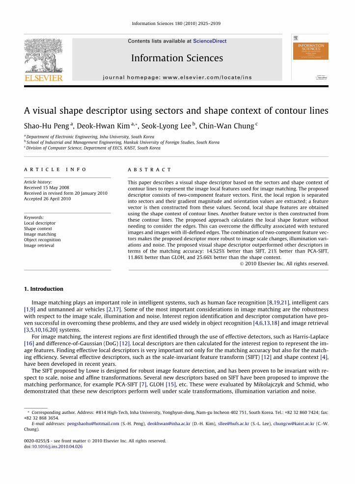
This paper presents a visual shape descriptor based on the sectors and shape context of contour lines. Fig. 1 shows a sche-matic of the process used to compute this descriptor.

The scale-space extreme points are first detected and the keypoint is located by removing the unstable ones. The keypointorientation is then assigned. For feature calculation, a circular region is then set around each keypoint. Finally, a sector-basedfeature vector and a feature vector based on shape context of contour lines are calculated. Both vectors are then combined toform a new descriptor.

For the sector-based feature vector, the region is separated into sectors of equal radii and angles similar to log-polar [22].The gradient magnitude and orientation of the pixels in each sector are calculated and mapped to a gradient histogram. Afeature vector is then generated using the histograms from all sectors around the keypoint. For the feature vector basedon the shape context of contour lines, the gray value of the keypoint is projected into the sea level of the geographicalmap. The altitude of each point in the circular region is then obtained by comparing the gray value of the point to that ofthe keypoint. Contour lines are then formed by grouping the points of similar altitude and the shape context of each contourline in the region is obtained. Similarly, the feature vector is generated using the shape context histograms of all contourlines. Finally, both feature vectors are combined to form a new descriptor.

The main contribution of the proposed method is as follows:

� The dimensionality of the descriptor is reduced using the sectors to calculate the gradient magnitude and orientation.� The shape features of the region without edge detection are obtained using the shape context of the contour lines.

A combination of the above feature vectors makes the proposed descriptor more robust with respect to image scale, illu-mination and noise. This new descriptor can achieve better matching accuracy and lower dimensionality than the SIFTdescriptor.

The remainder of this paper is organized as follows: Section 2 presents the background of the paper. Section 3 introducesthe new approach. The experiments and conclusions are discussed in Sections 4 and 5, respectively.

2. Background

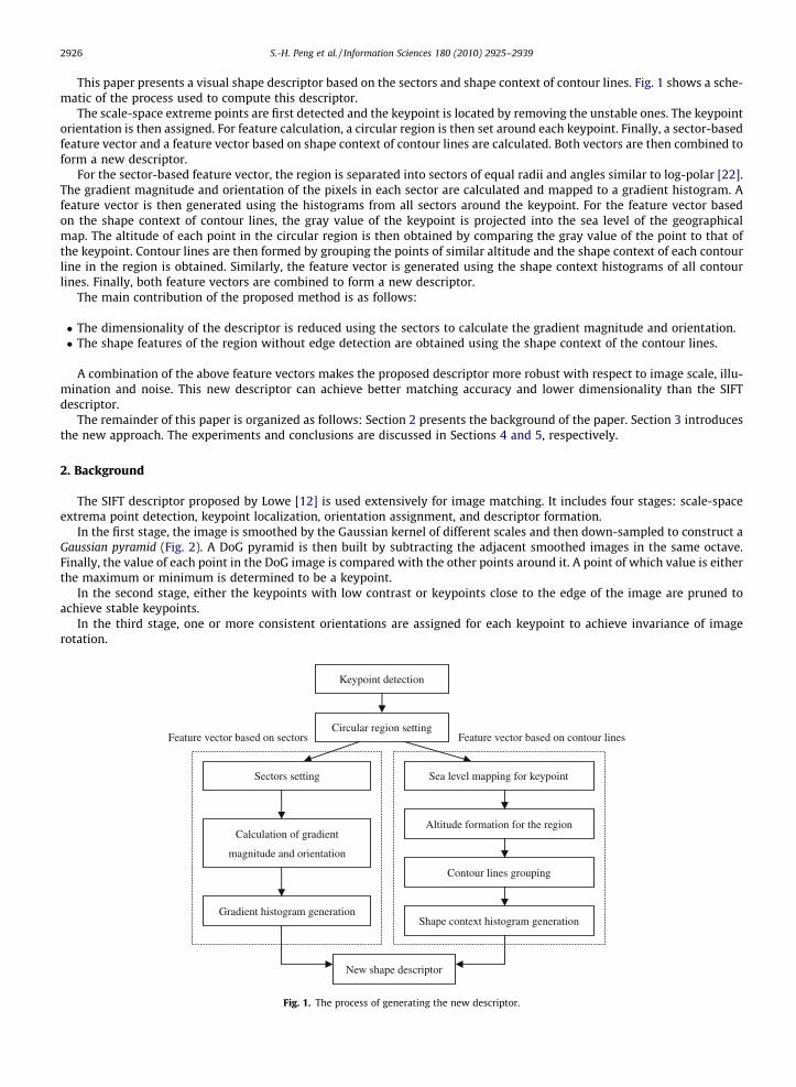
The SIFT descriptor proposed by Lowe [12] is used extensively for image matching. It includes four stages: scale-spaceextrema point detection, keypoint localization, orientation assignment, and descriptor formation.

In the first stage, the image is smoothed by the Gaussian kernel of different scales and then down-sampled to construct aGaussian pyramid (Fig. 2). A DoG pyramid is then built by subtracting the adjacent smoothed images in the same octave.Finally, the value of each point in the DoG image is compared with the other points around it. A point of which value is eitherthe maximum or minimum is determined to be a keypoint.

In the second stage, either the keypoints with low contrast or keypoints close to the edge of the image are pruned toachieve stable keypoints.

In the third stage, one or more consistent orientations are assigned for each keypoint to achieve invariance of imagerotation.

Feature vector based on contour lines Feature vector based on sectors

Keypoint detection

Circular region setting

Sectors setting

Calculation of gradient

magnitude and orientation

Gradient histogram generation

Sea level mapping for keypoint

Altitude formation for the region

Contour lines grouping

Shape context histogram generation

New shape descriptor

Fig. 1. The process of generating the new descriptor.

σ

kσ

2k σ

3k σ

4k σ

2k σ

3k σ

4k σ

5k σ

6k σ

Down sample

σ is the smooth scale of octave 1, interval 1.

1k >

……

Octave 1 Octave 2

……

Fig. 2. The process of building the Gaussian pyramid.

S.-H. Peng et al. / Information Sciences 180 (2010) 2925–2939 2927

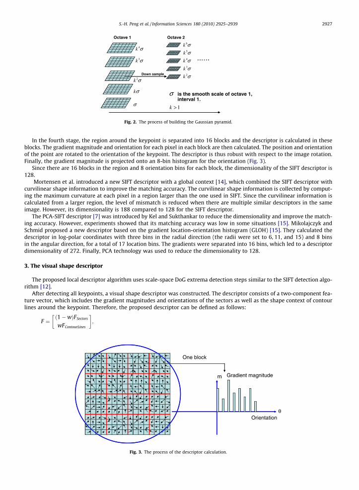
In the fourth stage, the region around the keypoint is separated into 16 blocks and the descriptor is calculated in theseblocks. The gradient magnitude and orientation for each pixel in each block are then calculated. The position and orientationof the point are rotated to the orientation of the keypoint. The descriptor is thus robust with respect to the image rotation.Finally, the gradient magnitude is projected onto an 8-bin histogram for the orientation (Fig. 3).

Since there are 16 blocks in the region and 8 orientation bins for each block, the dimensionality of the SIFT descriptor is128.

Mortensen et al. introduced a new SIFT descriptor with a global context [14], which combined the SIFT descriptor withcurvilinear shape information to improve the matching accuracy. The curvilinear shape information is collected by comput-ing the maximum curvature at each pixel in a region larger than the one used in SIFT. Since the curvilinear information iscalculated from a larger region, the level of mismatch is reduced when there are multiple similar descriptors in the sameimage. However, its dimensionality is 188 compared to 128 for the SIFT descriptor.

The PCA-SIFT descriptor [7] was introduced by Kel and Sukthankar to reduce the dimensionality and improve the match-ing accuracy. However, experiments showed that its matching accuracy was low in some situations [15]. Mikolajczyk andSchmid proposed a new descriptor based on the gradient location-orientation histogram (GLOH) [15]. They calculated thedescriptor in log-polar coordinates with three bins in the radial direction (the radii were set to 6, 11, and 15) and 8 binsin the angular direction, for a total of 17 location bins. The gradients were separated into 16 bins, which led to a descriptordimensionality of 272. Finally, PCA technology was used to reduce the dimensionality to 128.

3. The visual shape descriptor

The proposed local descriptor algorithm uses scale-space DoG extrema detection steps similar to the SIFT detection algo-rithm [12].

After detecting all keypoints, a visual shape descriptor was constructed. The descriptor consists of a two-component fea-ture vector, which includes the gradient magnitudes and orientations of the sectors as well as the shape context of contourlines around the keypoint. Therefore, the proposed descriptor can be defined as follows:

F ¼ð1�wÞFSectors

wFContourLines

� �;

m

Orientation

Gradient magnitude

One block

θ

Fig. 3. The process of the descriptor calculation.

2928 S.-H. Peng et al. / Information Sciences 180 (2010) 2925–2939

where FSectors is a 64-dimensional feature vector based on sectors, FContourLines is a 48-dimensional feature vector based on thelocal shape context, and w is the weight of two components according to user’s preference [11]. Hence, the proposed descrip-tor algorithm consists of three parts:

1. Find the feature vector using the gradient magnitude and orientation of pixels in the sectors around the keypoint.2. Find the feature vector using the shape context of the contour lines in a circular region centered at the keypoint.3. Combine both feature vectors to construct the visual shape descriptor.

First, a circular region is defined from which a two-component feature vector is extracted. Since the keypoint is detectedby the DoG detector [12], within different scales, the size of the circular region is defined as being relative to the scale of thekeypoint. The keypoint is also set as the center of the circular region because it is the most stable point in that region. There-fore, the radius of the circular region is set by the following equation:

R ¼ D � S; ð1Þ

where D is an experimentally determined multiplier, and S is a smoothing scale of the octave that the keypoint belongs to.Fig. 4 shows the circular region centered at the keypoint.

3.1. Feature vector based on sectors

In this section, the gradient magnitude and the orientation are extracted in Cartesian coordinates. However, instead ofusing Cartesian coordinates to separate the local region into 4-by-4 sub-regions [12], the local region is separated accordingto the sectors to reduce the dimensionality of the descriptor. Since the points close to the keypoint are more important thanthose farther away from it, the former can be viewed within small grids, whereas the latter can be viewed within large gridsusing polar coordinates to separate the circular region. Furthermore, a Gaussian weighting function with r equal to R is as-signed to each point to emphasize that the points are close to the keypoint. Therefore, the size of the grid can be enlarged toreduce the dimensionality of the descriptor without degrading its performance.

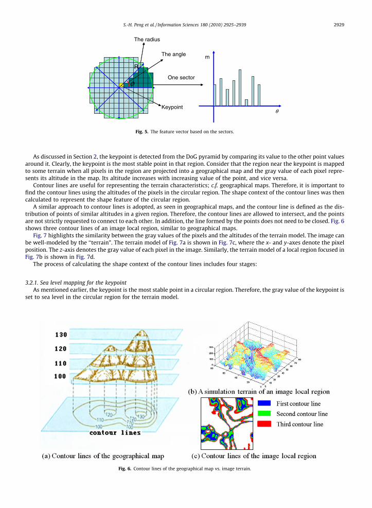
The circular region is separated into N sectors. A sector is a sub-region divided by the same angle and radius (Fig. 5). Thegradient magnitudes and orientations of the points in the sector are then calculated to form a histogram with M bins. Thegradient magnitude and orientation can be computed as follows:

mðx; yÞ ¼ffiffiffiffiffiffiffiffiffiffiffiffiffiffiffiffiffiffiffiffiffiffiffiffiffiffiffiffiffiffiffiffiffiffiffiffiffiffiffiffiffiffiffiffiffiffiffiffiffiffiffiffiffiffiffiffiffiffiffiffiffiffiffiffiffiffiffiffiffiffiffiffiffiffiffiffiffiffiffiffiffiffiffiffiffiffiffiffiffiffiffiffiffiffiffiffiffiffiffiffiffiffiffiffiffiffiffiffiffiffiffiffiffiffiffiffiðLðxþ 1; yÞ � Lðx� 1; yÞÞ2 þ ðLðx; yþ 1Þ � Lðx; y� 1ÞÞ2

q; ð2Þ

hðx; yÞ ¼ tan�1ðLðx; yþ 1Þ � Lðx; y� 1ÞLðxþ 1; yÞ � Lðx� 1; yÞÞ; ð3Þ

where x and y are the Cartesian coordinates of a point, m(x,y) is its gradient magnitude, h(x,y) is its orientation, and L(x,y) isits gray value. For each point in the sector, its gradient magnitude is mapped to the histogram bins corresponding to its ori-entation. Note that the position and orientation of the point are aligned to the orientation of the keypoint, invariance withrespect to the image rotation. Finally, all histograms of N sectors around the keypoint are concatenated to form the featurevector FSectors with N*M-dimension.

3.2. The shape context of the contour lines

Mikolajczyk and Schmid [15] showed that the shape context [4] achieved high performance for the images with clearedges. However, its performance suffered when applied to textured scenes or ill-defined edge images. Our innovative ap-proach utilizes the shape context in the circular region without edge detection to overcome the performance problems asso-ciated with the problematic edges of textured scenes.

The radius

Keypoint

Fig. 4. The circular region.

The radius

The angle

Keypoint

m

θ

One sector

R

φ

R

φ

Fig. 5. The feature vector based on the sectors.

S.-H. Peng et al. / Information Sciences 180 (2010) 2925–2939 2929

As discussed in Section 2, the keypoint is detected from the DoG pyramid by comparing its value to the other point valuesaround it. Clearly, the keypoint is the most stable point in that region. Consider that the region near the keypoint is mappedto some terrain when all pixels in the region are projected into a geographical map and the gray value of each pixel repre-sents its altitude in the map. Its altitude increases with increasing value of the point, and vice versa.

Contour lines are useful for representing the terrain characteristics; c.f. geographical maps. Therefore, it is important tofind the contour lines using the altitudes of the pixels in the circular region. The shape context of the contour lines was thencalculated to represent the shape feature of the circular region.

A similar approach to contour lines is adopted, as seen in geographical maps, and the contour line is defined as the dis-tribution of points of similar altitudes in a given region. Therefore, the contour lines are allowed to intersect, and the pointsare not strictly requested to connect to each other. In addition, the line formed by the points does not need to be closed. Fig. 6shows three contour lines of an image local region, similar to geographical maps.

Fig. 7 highlights the similarity between the gray values of the pixels and the altitudes of the terrain model. The image canbe well-modeled by the ‘‘terrain”. The terrain model of Fig. 7a is shown in Fig. 7c, where the x- and y-axes denote the pixelposition. The z-axis denotes the gray value of each pixel in the image. Similarly, the terrain model of a local region focused inFig. 7b is shown in Fig. 7d.

The process of calculating the shape context of the contour lines includes four stages:

3.2.1. Sea level mapping for the keypointAs mentioned earlier, the keypoint is the most stable point in a circular region. Therefore, the gray value of the keypoint is

set to sea level in the circular region for the terrain model.

Fig. 6. Contour lines of the geographical map vs. image terrain.

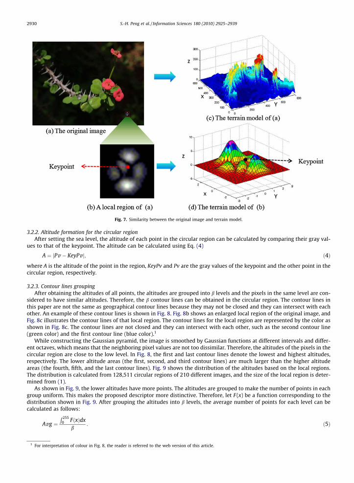
Fig. 7. Similarity between the original image and terrain model.

2930 S.-H. Peng et al. / Information Sciences 180 (2010) 2925–2939

3.2.2. Altitude formation for the circular regionAfter setting the sea level, the altitude of each point in the circular region can be calculated by comparing their gray val-

ues to that of the keypoint. The altitude can be calculated using Eq. (4)

1 For

A ¼ jPv � KeyPv j; ð4Þ

where A is the altitude of the point in the region, KeyPv and Pv are the gray values of the keypoint and the other point in thecircular region, respectively.

3.2.3. Contour lines groupingAfter obtaining the altitudes of all points, the altitudes are grouped into b levels and the pixels in the same level are con-

sidered to have similar altitudes. Therefore, the b contour lines can be obtained in the circular region. The contour lines inthis paper are not the same as geographical contour lines because they may not be closed and they can intersect with eachother. An example of these contour lines is shown in Fig. 8. Fig. 8b shows an enlarged local region of the original image, andFig. 8c illustrates the contour lines of that local region. The contour lines for the local region are represented by the color asshown in Fig. 8c. The contour lines are not closed and they can intersect with each other, such as the second contour line(green color) and the first contour line (blue color).1

While constructing the Gaussian pyramid, the image is smoothed by Gaussian functions at different intervals and differ-ent octaves, which means that the neighboring pixel values are not too dissimilar. Therefore, the altitudes of the pixels in thecircular region are close to the low level. In Fig. 8, the first and last contour lines denote the lowest and highest altitudes,respectively. The lower altitude areas (the first, second, and third contour lines) are much larger than the higher altitudeareas (the fourth, fifth, and the last contour lines). Fig. 9 shows the distribution of the altitudes based on the local regions.The distribution is calculated from 128,511 circular regions of 210 different images, and the size of the local region is deter-mined from (1).

As shown in Fig. 9, the lower altitudes have more points. The altitudes are grouped to make the number of points in eachgroup uniform. This makes the proposed descriptor more distinctive. Therefore, let F (x) be a function corresponding to thedistribution shown in Fig. 9. After grouping the altitudes into b levels, the average number of points for each level can becalculated as follows:

Avg ¼R 255

0 FðxÞdxb

: ð5Þ

interpretation of colour in Fig. 8, the reader is referred to the web version of this article.

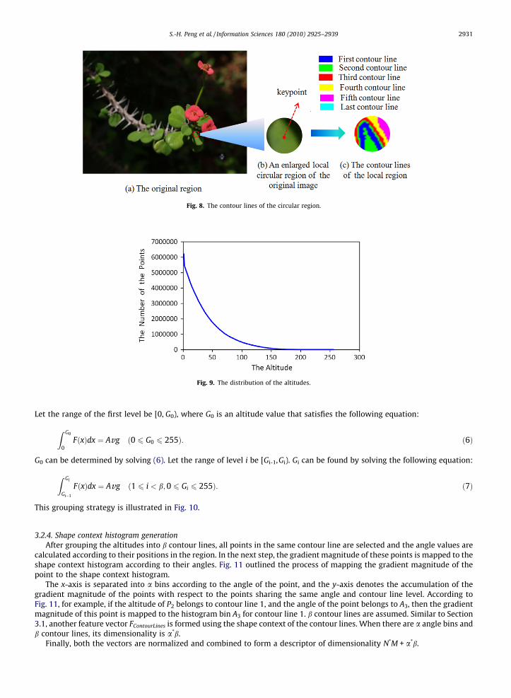
Fig. 8. The contour lines of the circular region.

Fig. 9. The distribution of the altitudes.

S.-H. Peng et al. / Information Sciences 180 (2010) 2925–2939 2931

Let the range of the first level be [0, G0), where G0 is an altitude value that satisfies the following equation:

Z G0

0FðxÞdx ¼ Avg ð0 6 G0 6 255Þ: ð6Þ

G0 can be determined by solving (6). Let the range of level i be [Gi-1,Gi). Gi can be found by solving the following equation:

Z Gi

Gi�1

FðxÞdx ¼ Avg ð1 6 i < b;0 6 Gi 6 255Þ: ð7Þ

This grouping strategy is illustrated in Fig. 10.

3.2.4. Shape context histogram generationAfter grouping the altitudes into b contour lines, all points in the same contour line are selected and the angle values are

calculated according to their positions in the region. In the next step, the gradient magnitude of these points is mapped to theshape context histogram according to their angles. Fig. 11 outlined the process of mapping the gradient magnitude of thepoint to the shape context histogram.

The x-axis is separated into a bins according to the angle of the point, and the y-axis denotes the accumulation of thegradient magnitude of the points with respect to the points sharing the same angle and contour line level. According toFig. 11, for example, if the altitude of P2 belongs to contour line 1, and the angle of the point belongs to A3, then the gradientmagnitude of this point is mapped to the histogram bin A3 for contour line 1. b contour lines are assumed. Similar to Section3.1, another feature vector FContourLines is formed using the shape context of the contour lines. When there are a angle bins andb contour lines, its dimensionality is a*b.

Finally, both the vectors are normalized and combined to form a descriptor of dimensionality N*M + a*b.

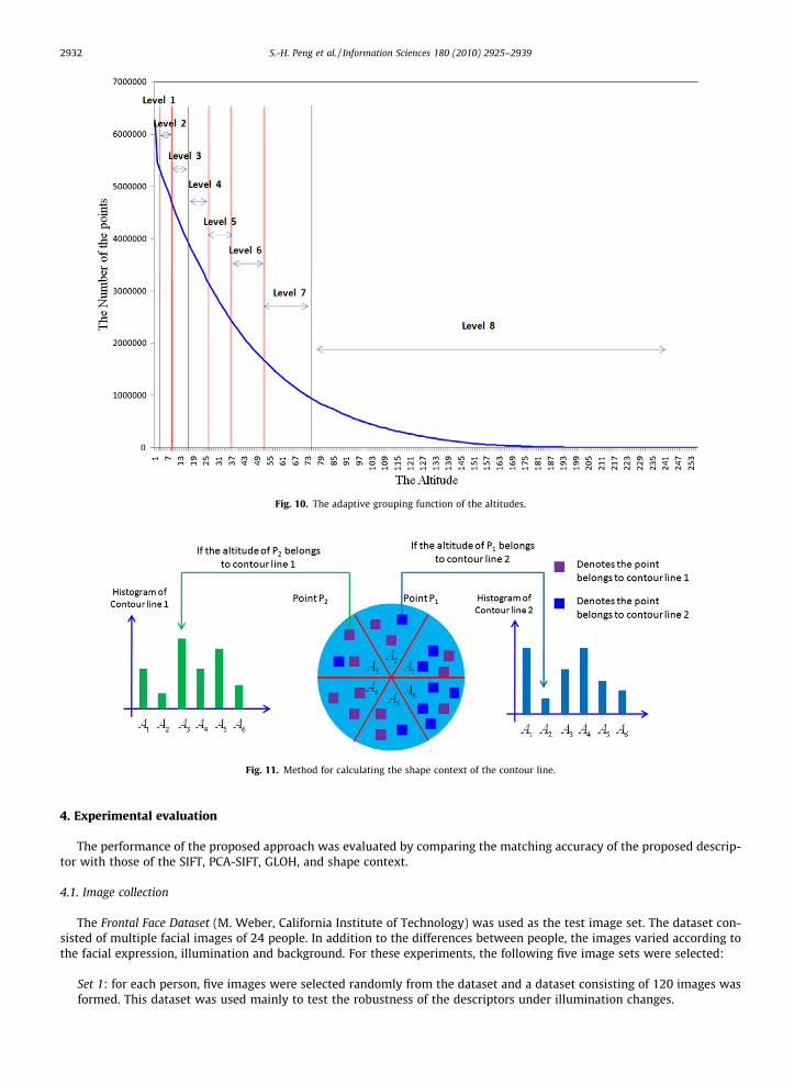
Fig. 10. The adaptive grouping function of the altitudes.

Fig. 11. Method for calculating the shape context of the contour line.

2932 S.-H. Peng et al. / Information Sciences 180 (2010) 2925–2939

4. Experimental evaluation

The performance of the proposed approach was evaluated by comparing the matching accuracy of the proposed descrip-tor with those of the SIFT, PCA-SIFT, GLOH, and shape context.

4.1. Image collection

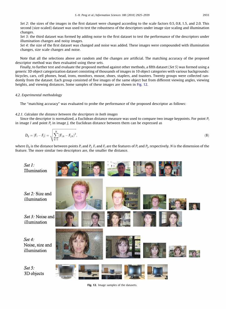
The Frontal Face Dataset (M. Weber, California Institute of Technology) was used as the test image set. The dataset con-sisted of multiple facial images of 24 people. In addition to the differences between people, the images varied according tothe facial expression, illumination and background. For these experiments, the following five image sets were selected:

Set 1: for each person, five images were selected randomly from the dataset and a dataset consisting of 120 images wasformed. This dataset was used mainly to test the robustness of the descriptors under illumination changes.

S.-H. Peng et al. / Information Sciences 180 (2010) 2925–2939 2933

Set 2: the sizes of the images in the first dataset were changed according to the scale factors 0.5, 0.8, 1.5, and 2.0. Thissecond (size-scaled) dataset was used to test the robustness of the descriptors under image size scaling and illuminationchanges.Set 3: the third dataset was formed by adding noise to the first dataset to test the performance of the descriptors underillumination changes and noisy images.Set 4: the size of the first dataset was changed and noise was added. These images were compounded with illuminationchanges, size scale changes and noise.

Note that all the selections above are random and the changes are artificial. The matching accuracy of the proposeddescriptor method was then evaluated using these sets.

Finally, to further test and evaluate the proposed method against other methods, a fifth dataset (Set 5) was formed using ageneric 3D object categorization dataset consisting of thousands of images in 10 object categories with various backgrounds:bicycles, cars, cell phones, head, irons, monitors, mouse, shoes, staplers, and toasters. Twenty groups were collected ran-domly from the dataset. Each group consisted of five images of the same object but from different viewing angles, viewingheights, and viewing distances. Some samples of these images are shown in Fig. 12.

4.2. Experimental methodology

The ‘‘matching accuracy” was evaluated to probe the performance of the proposed descriptor as follows:

4.2.1. Calculate the distance between the descriptors in both imagesSince the descriptor is normalized, a Euclidean distance measure was used to compare two image keypoints. For point Pi

in image I and point Pj in image J, the Euclidean distance between them can be expressed as

Dij ¼ jFi � Fjj ¼

ffiffiffiffiffiffiffiffiffiffiffiffiffiffiffiffiffiffiffiffiffiffiffiffiffiffiffiffiffiffiffiffiXN

k¼1

ðFi;k � Fj;kÞ2vuut ; ð8Þ

where Dij is the distance between points Pi and Pj. Fi and Fj are the features of Pi and Pj, respectively. N is the dimension of thefeature. The more similar two descriptors are, the smaller the distance.

Fig. 12. Image samples of the datasets.

2934 S.-H. Peng et al. / Information Sciences 180 (2010) 2925–2939

4.2.2. Calculate the number of matching image pairsFor a single keypoint Pi in image I, the distance values between Pi and all keypoints in the other image J were calculated.

The distances were ranked in order of closest to farthest. To determine if Pi is matched to any point in image J, ambiguityrejection metric is used, which is the ratio of the closest to the second closest distance. If the ratio is smaller than 0.8, theimage pair I and J are considered to be matched. Therefore, to match the two images, I and J, the number of matching pointpairs between the images is counted. The more matching point pairs found, the more similar the two images.

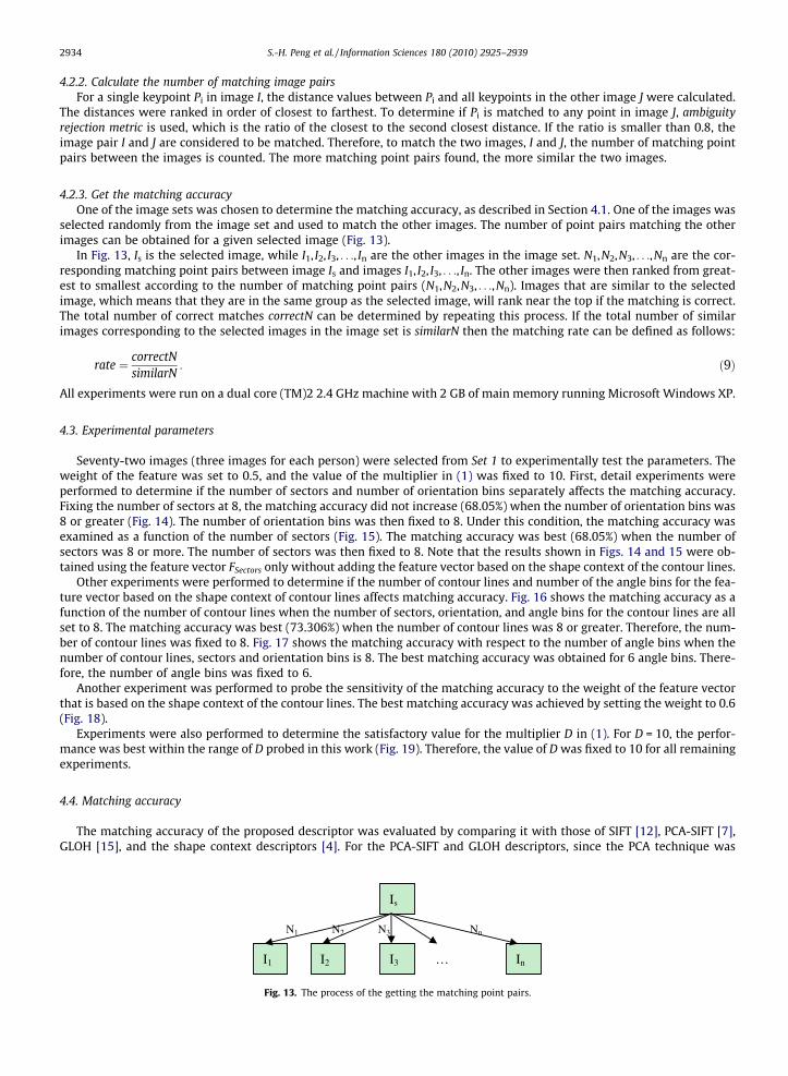
4.2.3. Get the matching accuracyOne of the image sets was chosen to determine the matching accuracy, as described in Section 4.1. One of the images was

selected randomly from the image set and used to match the other images. The number of point pairs matching the otherimages can be obtained for a given selected image (Fig. 13).

In Fig. 13, Is is the selected image, while I1, I2, I3, . . ., In are the other images in the image set. N1,N2,N3, . . .,Nn are the cor-responding matching point pairs between image Is and images I1, I2, I3, . . ., In. The other images were then ranked from great-est to smallest according to the number of matching point pairs (N1,N2,N3, . . .,Nn). Images that are similar to the selectedimage, which means that they are in the same group as the selected image, will rank near the top if the matching is correct.The total number of correct matches correctN can be determined by repeating this process. If the total number of similarimages corresponding to the selected images in the image set is similarN then the matching rate can be defined as follows:

rate ¼ correctNsimilarN

: ð9Þ

All experiments were run on a dual core (TM)2 2.4 GHz machine with 2 GB of main memory running Microsoft Windows XP.

4.3. Experimental parameters

Seventy-two images (three images for each person) were selected from Set 1 to experimentally test the parameters. Theweight of the feature was set to 0.5, and the value of the multiplier in (1) was fixed to 10. First, detail experiments wereperformed to determine if the number of sectors and number of orientation bins separately affects the matching accuracy.Fixing the number of sectors at 8, the matching accuracy did not increase (68.05%) when the number of orientation bins was8 or greater (Fig. 14). The number of orientation bins was then fixed to 8. Under this condition, the matching accuracy wasexamined as a function of the number of sectors (Fig. 15). The matching accuracy was best (68.05%) when the number ofsectors was 8 or more. The number of sectors was then fixed to 8. Note that the results shown in Figs. 14 and 15 were ob-tained using the feature vector FSectors only without adding the feature vector based on the shape context of the contour lines.

Other experiments were performed to determine if the number of contour lines and number of the angle bins for the fea-ture vector based on the shape context of contour lines affects matching accuracy. Fig. 16 shows the matching accuracy as afunction of the number of contour lines when the number of sectors, orientation, and angle bins for the contour lines are allset to 8. The matching accuracy was best (73.306%) when the number of contour lines was 8 or greater. Therefore, the num-ber of contour lines was fixed to 8. Fig. 17 shows the matching accuracy with respect to the number of angle bins when thenumber of contour lines, sectors and orientation bins is 8. The best matching accuracy was obtained for 6 angle bins. There-fore, the number of angle bins was fixed to 6.

Another experiment was performed to probe the sensitivity of the matching accuracy to the weight of the feature vectorthat is based on the shape context of the contour lines. The best matching accuracy was achieved by setting the weight to 0.6(Fig. 18).

Experiments were also performed to determine the satisfactory value for the multiplier D in (1). For D = 10, the perfor-mance was best within the range of D probed in this work (Fig. 19). Therefore, the value of D was fixed to 10 for all remainingexperiments.

4.4. Matching accuracy

The matching accuracy of the proposed descriptor was evaluated by comparing it with those of SIFT [12], PCA-SIFT [7],GLOH [15], and the shape context descriptors [4]. For the PCA-SIFT and GLOH descriptors, since the PCA technique was

NnN3N2N1

I1 I2 I3 In

Is

…

Fig. 13. The process of the getting the matching point pairs.

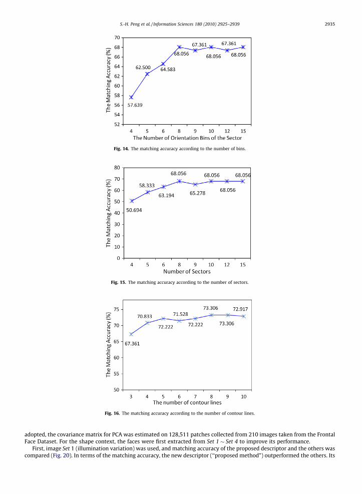
Fig. 14. The matching accuracy according to the number of bins.

Fig. 15. The matching accuracy according to the number of sectors.

Fig. 16. The matching accuracy according to the number of contour lines.

S.-H. Peng et al. / Information Sciences 180 (2010) 2925–2939 2935

adopted, the covariance matrix for PCA was estimated on 128,511 patches collected from 210 images taken from the FrontalFace Dataset. For the shape context, the faces were first extracted from Set 1 � Set 4 to improve its performance.

First, image Set 1 (illumination variation) was used, and matching accuracy of the proposed descriptor and the others wascompared (Fig. 20). In terms of the matching accuracy, the new descriptor (‘‘proposed method”) outperformed the others. Its

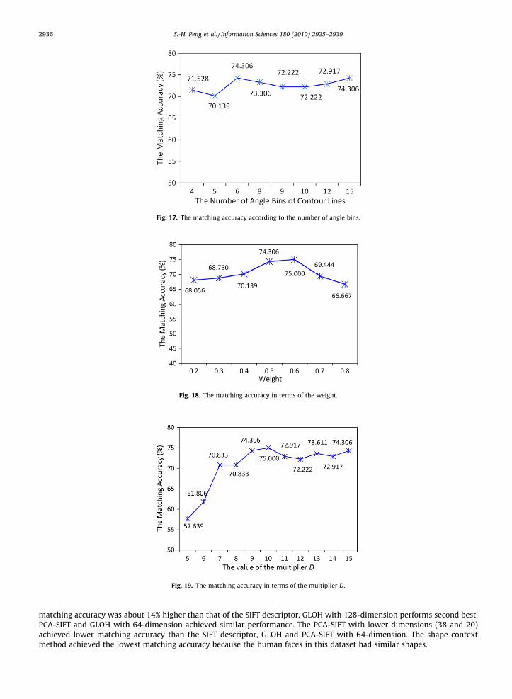
Fig. 17. The matching accuracy according to the number of angle bins.

Fig. 18. The matching accuracy in terms of the weight.

Fig. 19. The matching accuracy in terms of the multiplier D.

2936 S.-H. Peng et al. / Information Sciences 180 (2010) 2925–2939

matching accuracy was about 14% higher than that of the SIFT descriptor. GLOH with 128-dimension performs second best.PCA-SIFT and GLOH with 64-dimension achieved similar performance. The PCA-SIFT with lower dimensions (38 and 20)achieved lower matching accuracy than the SIFT descriptor, GLOH and PCA-SIFT with 64-dimension. The shape contextmethod achieved the lowest matching accuracy because the human faces in this dataset had similar shapes.

S.-H. Peng et al. / Information Sciences 180 (2010) 2925–2939 2937

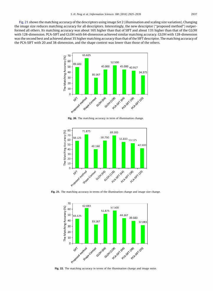
Fig. 21 shows the matching accuracy of the descriptors using image Set 2 (illumination and scaling size variation). Changingthe image size reduces matching accuracy for all descriptors. Interestingly, the new descriptor (‘‘proposed method”) outper-formed all others. Its matching accuracy was about 16% higher than that of SIFT and about 13% higher than that of the GLOHwith 128-dimension. PCA-SIFT and GLOH with 64-dimension achieved similar matching accuracy. GLOH with 128-dimensionwas the second best and achieved about 3% higher matching accuracy than that of the SIFT descriptor. The matching accuracy ofthe PCA-SIFT with 20 and 38-dimension, and the shape context was lower than those of the others.

Fig. 20. The matching accuracy in term of illumination change.

Fig. 21. The matching accuracy in terms of the illumination change and image size change.

Fig. 22. The matching accuracy in terms of the illumination change and image noise.

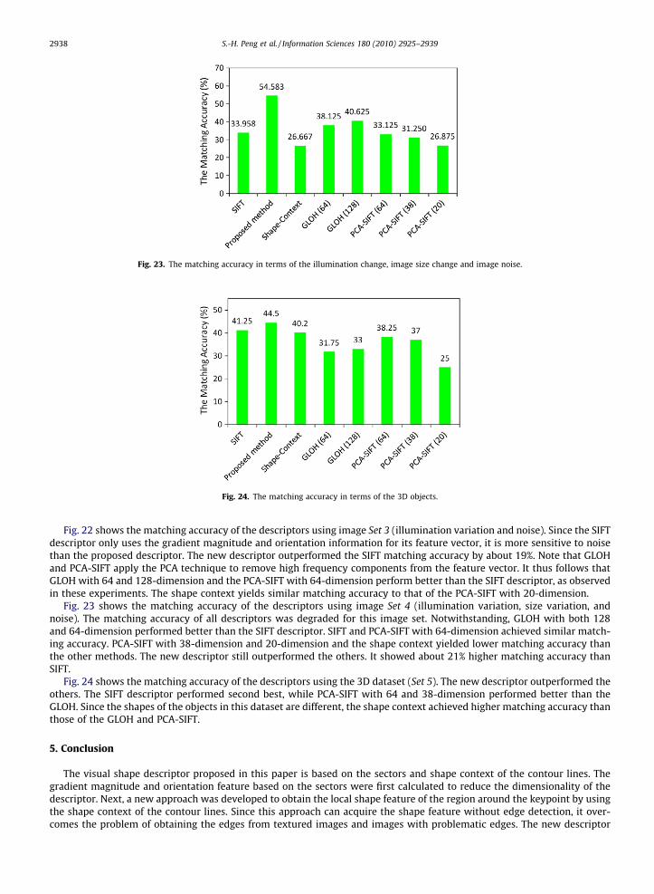
Fig. 23. The matching accuracy in terms of the illumination change, image size change and image noise.

Fig. 24. The matching accuracy in terms of the 3D objects.

2938 S.-H. Peng et al. / Information Sciences 180 (2010) 2925–2939

Fig. 22 shows the matching accuracy of the descriptors using image Set 3 (illumination variation and noise). Since the SIFTdescriptor only uses the gradient magnitude and orientation information for its feature vector, it is more sensitive to noisethan the proposed descriptor. The new descriptor outperformed the SIFT matching accuracy by about 19%. Note that GLOHand PCA-SIFT apply the PCA technique to remove high frequency components from the feature vector. It thus follows thatGLOH with 64 and 128-dimension and the PCA-SIFT with 64-dimension perform better than the SIFT descriptor, as observedin these experiments. The shape context yields similar matching accuracy to that of the PCA-SIFT with 20-dimension.

Fig. 23 shows the matching accuracy of the descriptors using image Set 4 (illumination variation, size variation, andnoise). The matching accuracy of all descriptors was degraded for this image set. Notwithstanding, GLOH with both 128and 64-dimension performed better than the SIFT descriptor. SIFT and PCA-SIFT with 64-dimension achieved similar match-ing accuracy. PCA-SIFT with 38-dimension and 20-dimension and the shape context yielded lower matching accuracy thanthe other methods. The new descriptor still outperformed the others. It showed about 21% higher matching accuracy thanSIFT.

Fig. 24 shows the matching accuracy of the descriptors using the 3D dataset (Set 5). The new descriptor outperformed theothers. The SIFT descriptor performed second best, while PCA-SIFT with 64 and 38-dimension performed better than theGLOH. Since the shapes of the objects in this dataset are different, the shape context achieved higher matching accuracy thanthose of the GLOH and PCA-SIFT.

5. Conclusion

The visual shape descriptor proposed in this paper is based on the sectors and shape context of the contour lines. Thegradient magnitude and orientation feature based on the sectors were first calculated to reduce the dimensionality of thedescriptor. Next, a new approach was developed to obtain the local shape feature of the region around the keypoint by usingthe shape context of the contour lines. Since this approach can acquire the shape feature without edge detection, it over-comes the problem of obtaining the edges from textured images and images with problematic edges. The new descriptor

S.-H. Peng et al. / Information Sciences 180 (2010) 2925–2939 2939

combines the gradient magnitude, orientation and shape context feature of the local region around the keypoint. Therefore,it represents richer feature information of the local region with lower dimension of 112, whereas the dimension of the SIFTdescriptor is 128. Experimental results demonstrate that the new visual shape descriptor is more robust than the others,namely SIFT, PCA-SIFT, and GLOH, in terms of the matching accuracy with respect to illumination variations, scale variations,and noise.

Acknowledgement

The authors thank the Editor and the anonymous reviewers for their valuable comments in improving the quality of thispaper. This research was supported in part by Basic Science Research Program through the National Research Foundation ofKorea (NRF) funded by the Ministry of Education, Science and Technology (Grant No. 2009-0081365), in part by the NationalResearch Foundation of Korea (NRF) grant funded by the Korea government (MEST) (R01-2008-000-20685-0) and in part bythe Ministry of Knowledge Economy (MKE) and Korea Institute for Advancement in Technology (KIAT) through theWorkforce Development Program in Strategic Technology.

References

[1] C.Y. Chen, H.M. Feng, Hybrid intelligent vision-based car-like vehicle backing systems design, Expert Systems with Applications 36 (2009) 7500–7509.[2] G. Conte, P. Doherty, An integrated UAV navigation system based on aerial image matching, in: IEEE Conference on Aerospace, Montana, USA, 2008, pp.

1–10.[3] A. El-ghazal, O. Basir, S. Belkasim, A consensus-based fusion algorithm in shape-based image retrieval, in: 10th International Conference on

Information Fusion, Québec City, 2007, pp. 1–8.[4] S.B. Elongie, J. Malik, J. Puzicha, Shape matching and object recognition using shape contexts, In: IEEE Transactions on Pattern Analysis and Machine

Intelligent, 2002, pp. 509–522.[5] J.J. Foo, R. Sinha, J. Zobel, SICO: a system for detection of near-duplicate image during search, in: IEEE International Conference of Multimedia and Expo,

Beijing, China, 2007, pp. 595–598.[6] R. Fergus, P. Perona, A. Zisserman, Object class recognition by unsupervised scale-invariant learning, in: IEEE Computer Society Conference on

Computer Vision and Pattern Recognition, Madison, Wisconsin, 2003, pp. 264–271.[7] Y. Ke1, R. Sukthankar, PCA-SIFT: a more distinctive representation for local image descriptors, in: IEEE Computer Society Conference on Image

Processing and Pattern Recognition, 2004, pp. 506–513.[8] Z.K. Huang, W.Z. Zhang, H.M. Huang, L.Y. Hou, Using gabor filters features for multi-pose face recognition in color images, in: Intelligent Information

Technology Application, 2008, pp. 399–402.[9] C. Liu, J. Chen, Y. Xu, F. Luo, Intelligent vehicle road recognition based on the CMOS camera, in: Vehicle Power and Propulsion Conference, 2008, pp. 1–5.

[10] D.H. Kim, J.W. Song, J.H. Lee, B.G. Choi, Support vector machine learning for region-based image retrieval with relevance feedback, ETRI Journal 29 (5)(2007) 700–702.

[11] D.H. Kim, S.H. Yu, A new region filtering and region weighting approach to relevance feedback in content-based image retrieval, The Journal of Systemsand Software 81 (2008) 1525–1538.

[12] D.G. Lowe, Distinctive image features from scale-invariant keypoint, Computer Vision 2 (2004) 91–110.[13] D.G. Lowe, Object recognition from local scale-invariant features, Computer Vision 2 (1999) 1150–1157.[14] E.N. Mortensen, H. Deng, L. Shapiro, A SIFT descriptor with global context, in: IEEE Computer Society Conference on Computer Vision and Pattern

Recognition, San Diego, CA, 2005, pp. 184–190.[15] K. Mikolajczyk, C. Schmid, A performance evaluation of local descriptors, IEEE Transactions on Pattern Analysis and Machine Intelligence 27 (2005)

1615–1630.[16] K. Mikolajczyk, C. Schmid, Indexing based on scale invariant interest points, Eighth IEEE International Conference on Computer Vision, Vancouver,

Canada, 2001, pp. 525–531.[17] X. Pan, D.Q. Deng, L.L. Jiang, S. Zhen, Vision-based approach angle and height estimation for UAV landing, Conference of Image and Signal Processing,

Cherbourg-Octeville, France, 2008, pp. 801–805.[18] L. Shao, T. Kadir, M. Brady, Geometric and photometric invariance distinctive regions detection, Information Sciences 177 (2007) 1088–1122.[19] F.Y. Shih, C.Y. Fu, K. Zhang, Multi-view face identification and pose estimation using B-spline interpolation, Information Sciences 169 (2005) 189–204.[20] W.T. Wong, F.Y. Shih, J. Liu, Shape-based image retrieval using support vector machines, Fourier descriptors and self-organizing maps, Information

Sciences 177 (2007) 1878–1891.[21] X.D. Xie, K.M. Lam, Elastic shape–texture matching for human face recognition, Pattern Recognition 41 (2008) 396–405.[22] S. Zokai, G. Wolberg, Image registration using log-polar mappings for recovery of large-scale similarity and projective transformations, IEEE

Transaction on Image Processing 14 (2005) 1422–1434.