A Visual Analytics System for Radio Frequency Fingerprinting-basedLocalization

Yi Han∗ Erich P. Stuntebeck† John T. Stasko‡ Gregory D. Abowd§

School of Interactive Computing & GVU CenterGeorgia Institute of Technology

ABSTRACT

Radio frequency (RF) fingerprinting-based techniques for localiza-tion are a promising approach for ubiquitous positioning systems,particularly indoors. By finding unique fingerprints of RF signalsreceived at different locations within a predefined area beforehand,whenever a similar fingerprint is subsequently seen again, the lo-calization system will be able to infer a user’s current location.However, developers of these systems face the problem of findingreliable RF fingerprints that are unique enough and adequately sta-ble over time. We present a visual analytics system that enablesdevelopers of these localization systems to visually gain insighton whether their collected datasets and chosen fingerprint featureshave the necessary properties to enable a reliable RF fingerprinting-based localization system. The system was evaluated by testing anddebugging an existing localization system.

Index Terms: H.5.2 [User Interfaces]: Graphical user interfaces(GUI)—; D.2.5 [Testing and Debugging]: Debugging aids—

1 INTRODUCTION

Tracking the location of people and objects inside of buildings hasbeen an active area of research for some years. The traditionalmeans of accomplishing this outdoors - GPS satellites - is unavail-able indoors since buildings block the satellite signals. One ap-proach researchers have taken in solving this problem is generatingtheir own indoor radio frequency (RF) signal(s) as a type of localGPS signal. Small tags, which can be thought of as ”indoor GPSreceivers” track some aspect of these locally generated RF signalsand use this information to locate themselves within the building.

Outdoor GPS receivers operate by triangulating their positionbased on the time of arrival of signals from multiple GPS satel-lites. There is typically line-of-sight between the GPS satellites andthe receivers, allowing predictable RF signal propagation. Indoors,RF signal propagation is very difficult to predict due to phenomenasuch as multi-path propagation, wherein the signal can propagatefrom transmitter to receiver via multiple paths by bouncing off wallsand furniture. Small movements in physical space can producelarge differences in the signal since the multiple paths may con-structively or destructively interfere at any given position. Thesephenomena are nearly impossible to predict a priori.

To address this problem, researchers have developed the methodof Radio frequency location fingerprinting. RF fingerprinting relieson measurements of relevant features of the signals at various dis-cretized locations. These measurements are taken when the systemis initially deployed. Later, when the system is in use, live mea-surements taken by the mobile tags are matched to the fingerprinted

∗e-mail: yihan@gatech.edu†e-mail: eps@gatech.edu‡e-mail: stasko@cc.gatech.edu§e-mail: abowd@gatech.edu

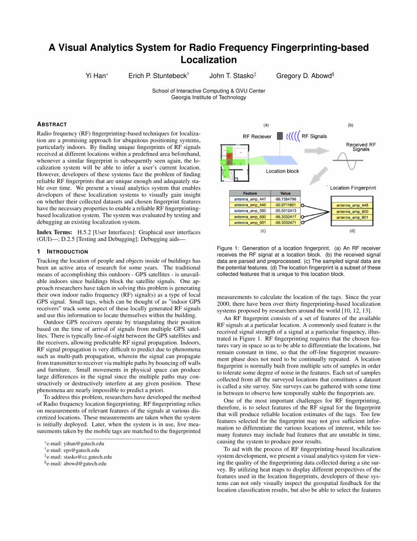
Figure 1: Generation of a location fingerprint. (a) An RF receiverreceives the RF signal at a location block. (b) the received signaldata are parsed and preprocessed. (c) The sampled signal data arethe potential features. (d) The location fingerprint is a subset of thesecollected features that is unique to this location block.

measurements to calculate the location of the tags. Since the year2000, there have been over thirty fingerprinting-based localizationsystems proposed by researchers around the world [10, 12, 13].

An RF fingerprint consists of a set of features of the availableRF signals at a particular location. A commonly used feature is thereceived signal strength of a signal at a particular frequency, illus-trated in Figure 1. RF fingerprinting requires that the chosen fea-tures vary in space so as to be able to differentiate the locations, butremain constant in time, so that the off-line fingerprint measure-ment phase does not need to be continually repeated. A locationfingerprint is normally built from multiple sets of samples in orderto tolerate some degree of noise in the features. Each set of samplescollected from all the surveyed locations that constitutes a datasetis called a site survey. Site surveys can be gathered with some timein between to observe how temporally stable the fingerprints are.

One of the most important challenges for RF fingerprinting,therefore, is to select features of the RF signal for the fingerprintthat will produce reliable location estimates of the tags. Too fewfeatures selected for the fingerprint may not give sufficient infor-mation to differentiate the various locations of interest, while toomany features may include bad features that are unstable in time,causing the system to produce poor results.

To aid with the process of RF fingerprinting-based localizationsystem development, we present a visual analytics system for view-ing the quality of the fingerprinting data collected during a site sur-vey. By utilizing heat maps to display different perspectives of thefeatures used in the location fingerprints, developers of these sys-tems can not only visually inspect the geospatial feedback for thelocation classification results, but also be able to select the features

to use by visually finding those that are temporally stable and spa-tially differentiable in a high dimensional feature space. When nec-essary, developers can even explore lower level details of any indi-vidual feature to see raw values and relationships to others througha multivariate visualization. Using our system, developers of local-ization systems can tell whether their datasets collected are capableof building good RF location fingerprints that can enable accuratelocation estimates over time.

The contribution of this work is to show how visual ana-lytics can support the development and practical deployment offingerprinting-based localization systems. We feel that this tool isa particularly good example of visual analytics because the mosteffective way to find a good location fingerprint is to combine thecomputational data analysis with an interactive geospatial visual-ization interface.

2 RELATED WORK

The RADAR system proposed by Bahl and Padmanabhan in 2000was the earliest RF fingerprinting-based localization system [3].The researchers were able to achieve a median of 2-3 meters ac-curacy indoors using Wi-Fi signals. Since then, researchers havereported over thirty systems using different RF signals or classifica-tion algorithms [10]. However, although these localization systemsare easy to deploy, the initial setup and calibration process for gen-erating the fingerprints is tedious and time consuming [11]. Theycan also be less reliable when the features used for the fingerprintsare not spatially differentiable and stable over time. Kaemarungsiand Padmanabhan studied the properties of Wi-Fi location finger-prints using received signal strength and learned that even the pres-ence of a human body can make a significant difference on the fin-gerprints [9]. Therefore, it is crucial to identify and remove unstablefeatures in the generated fingerprints to maintain the reliability ofthe localization system over time.

Visualizing RF signals on a geospatial map using heat maps isprevalent in 802.11 WLAN site survey tools for optimizing Wi-Finetwork coverage. Ekahau Site Survey took a step forward to notonly visualize the propagation of Wi-Fi signals but also integratethe output to power their Real-Time Location Tracking System [5].Nevertheless, this consumer-facing site survey tool cannot supportmore advanced visual debugging functions on feature selection andlocation fingerprint classification.

Spectrum analyzers for identifying physical locations of signalsources also require visualizing signals on a geospatial map andclassifying them. Tektronix’s RFHawk Signal Hunter identifiespotential malicious RF signals by singling them out from knownsignals [14]. The malicious signal will then be documented on ageospatial map with a color-coded wave form or signal strengthicon for later reference. However, as the tool did not aim to sup-port location fingerprinting, the wave form icons on the map havelittle power to show the individual feature differences for buildingspatially differentiable location fingerprints.

Andrienko and Andrienko used interactive cartographic visual-ization to output results of the C4.5 classification learning algorithmfor knowledge discovery [1]. Their work suggested that interac-tive visual facilities that allow an analyst to manipulate variablesand immediately observe the resulting changes in a map is effec-tive for geospatial data analysis. Our visual analytics system tooka step further for the K-nearest neighbor classification algorithm asto even visualize the intermediate steps of the algorithm for indoorlocalization.

Our system was developed with data from the PowerLine Posi-tioning localization system (PLP) [12]. PLP injects an RF signalinto the power lines of a residential building and uses the powerlines as a giant antenna for propagating the signals. The mobilewireless tag can then use this signal’s characteristics as the featureset to fingerprint locations within the area where the power lines can

reach. The latest revision of this system utilizes a feature set thatsamples 44 different frequencies of the amplitudes of the signal forlocation fingerprinting [13]. All the illustrations shown in this pa-per are either using the original data of this system or a modifiedversion of it. The data of the system was gathered in a residentiallaboratory on a university campus. This lab has a similar layout andelectrical infrastructure as a common residential house. We markedout one meter by one meter blocks on the floor, producing 66 dif-ferent locations for our site survey.

In the next section, we will discuss the current problems in build-ing a good location fingerprint with the existing, analytic text-basedmachine learning approaches. In Section 4, we will briefly providean overview of the visualization interface. We will present a sce-nario that demonstrates how our visual analytics system works inSection 5. More details and example uses of the visualization willbe discussed in Section 6.

3 RADIO FREQUENCY FINGERPRINTING-BASED LOCALIZA-TION

3.1 System Development ProcedureThe procedure to build a location fingerprinting system can beroughly decomposed into three steps. The system presented hereis focused on supporting the last two steps.

1. The first step is to gather the datasets and feature sets that canbe potentially used to generate a location fingerprint database.This requires a tedious site survey that maps where the RFsignals are gathered in the real world.

2. The second step is to find the right set of RF signal character-istics for the fingerprints. This step involves feature selectionand building the fingerprints with the selected features.

3. The last step is to test the collected fingerprints with RF sig-nals received at random locations in the surveyed area (ran-dom fingerprints). The signal data will be input to the local-ization system to see if it can accurately find the true loca-tions of these random fingerprints through classification algo-rithms.

3.2 Problems and Challenges for Building Location Fin-gerprints

The generation of the location fingerprint database on a radio maprequires a site survey in advance. This survey normally requiresa user to manually tell the system where they are so that the sys-tem can learn the RF signal pattern at that specific location. Thisprocess can be very tedious and time-consuming. For example, inthe PowerLine Positioning system, the time to survey each locationwith the full 44 features can take around 2 minutes. It takes about 2hours to survey 66 locations in practice. If the location fingerprintsare unstable over time, users might need to conduct the site surveyagain later to calibrate the system.

One major challenge is how to find the best features that canbe used for building a set of good location fingerprints. In prac-tice, we would like to use as few features as possible to build thefingerprints. There are two reasons for this. First, the fewer thefeatures means that the training time and classification time for themachine learning algorithm can be shorter. For real-time localiza-tion, this can be very crucial. Second, fewer numbers of features fora fingerprint can result in a shorter time required for the site surveydata collection process. Half the number of features needed meanshalf the time for this tedious preprocessing procedure. However,the fewer the features used, the less likely individual fingerprintswill be unique, resulting in higher overall classification error. Sothe technical challenge is how to find a balancing point where asmaller set of features can be used while the system is still capableto accurately classify a certain area of interest.

3.3 Problems with the Current ApproachThe current approach used by localization developers to prove theserequired properties of the location fingerprints are achieved is byrunning machine learning algorithms with the fingerprints gatheredat different times. The outputs of this approach are the text-basedclassification accuracy and misclassified locations when they testthe fingerprints. There are several problems with this approach:

First of all, it is not easy to tell how each feature composed in afingerprint is contributing to the overall classification results. Forpractical applications, one might have a few locations that are moreimportant to be always classified with high accuracy while otherlocations are fine to be occasionally incorrect. There are many fea-ture selection algorithms to analyze how each feature can build upthe overall accuracy. However, different features may improve theclassification accuracies of different areas on the radio map whilethey all improved the same overall accuracy.

Additionally, if there are a few locations that are always misclas-sified by the algorithm, it is very difficult to dig down into the multi-dimensional raw feature sets to identify the problem. Is it causedby a problematic training data set gathered or is the current finger-print just not unique enough to correctly classify this location? Ifthis kind of debugging cannot be performed, it is very hard for alocation fingerprinting system to be practically deployed with thedesired accuracy for any specified area of interest. Moreover, dur-ing the site survey process, sometimes there are RF interferences.These interference events can jeopardize the reliability of the pro-duced fingerprints that should be mostly accurate for the most com-mon cases. Moreover, it is not easy to find extreme cases whendealing with multidimensional data.

The requirements can be summed up in two major questions thatneed to be answered:

1. How do we effectively find a set of location fingerprints thatare good enough for certain areas of interest?

2. If there are some locations that consistently receive inaccurateclassifications, how do we find the problem?

To answer these two questions, several capabilities are required.

1. Test new unknown fingerprints with a preview of classifica-tion results on a map.

2. Test different subsets of features that can be used to composethe location fingerprints.

3. Examine the raw data of each individual feature for the fin-gerprints at different locations and its temporal stability.

4. Examine the spatial variance between locations in the highdimensional feature space of the fingerprints.

The design of the visual analytics system directly addresses thesequestions and targets these tasks. However, in subsequent use of thesystem, several unexpected interesting insights of the datasets andfeatures were also discovered.

4 VISUAL ANALYTICS SYSTEM OVERVIEW

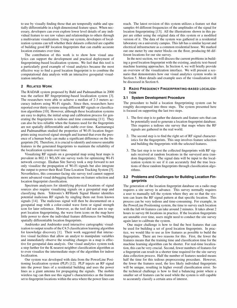
4.1 Interface OverviewThe interface of the system contains four main panels as shown inFigure 2.

1. Dataset selection This panel allows developers to select thedatasets to be viewed or used. Datasets can be selected in-dividually or with others according to the operation context.For example, multiple datasets should be selected when oneattempts to calculate the standard deviation between them

Figure 2: The four panels of our visual analytics system interface.

whereas only a single selection is needed when one attemptsto view the raw feature value of a specific dataset. To the rightof the dataset selection combo box is a timeline that showswhen the datasets selected were collected. When a dataset isselected, the oval symbol representing it will be highlighted inblue. Each oval symbol on the top or bottom of the timelinerepresents a data set gathered.

2. Feature selection This panel allows developers to select thefeatures to use to compose the fingerprints. It supports singleor multiple selections according to the context of use.

3. Main map The main map panel is the display area for thegeospatial visualization. A preloaded map is displayed in thebackground to provide the geospatial context for the visual-ization. By selecting different viewing perspectives, datasetsand feature sets, this panel shows a grid-based heat map forthe selected parameters. The heat map representation is veryuseful in showing the relative query results between differentlocations on the map. This visualization technique is partic-ularly effective for examining a fingerprinting-based localiza-tion system because we are most interested in the spatial dif-ferentiability of the location fingerprints. At the bottom ofthis perspective is the status bar. It shows the current selectedfeature set, the mouse interaction mode and information aboutthe heat map being presented.

4. Perspective control This panel is used to control the view-ing perspectives. The system provides three different viewingperspectives, each showing a different type of information ofthe datasets, features and complementing each other when thedeveloper intends to drill down to a specific problem.

• Data Variance Perspective (Figure 3) shows the raw data ofall the datasets with their corresponding feature sets.

• Spatial Variance Perspective (Figure 8) shows the spatialvariance of between fingerprints in the high dimensional fea-ture space using the selected features.

• Test Classification Perspective (Figure 4) provides a geospa-tial representation to show the results of the location classifi-cation using the generated fingerprints.

We use a green-gray-red color scheme for the heat maps dis-played in the main map panel. Green indicates better results andred indicates worse. As for other colors used in the system, weavoid using green or red to avoid any semantic confusion.

Feature Value Rankantenna amp 447 -56.7354796 2antenna amp 448 -56.9711881 1antenna amp 500 -55.5012413 5antenna amp 600 -56.3032417 4antenna amp 601 -56.3032471 3

Table 1: Feature transformation for ranking version of PLP

5 SCENARIO

5.1 PLP Ranking Dataset

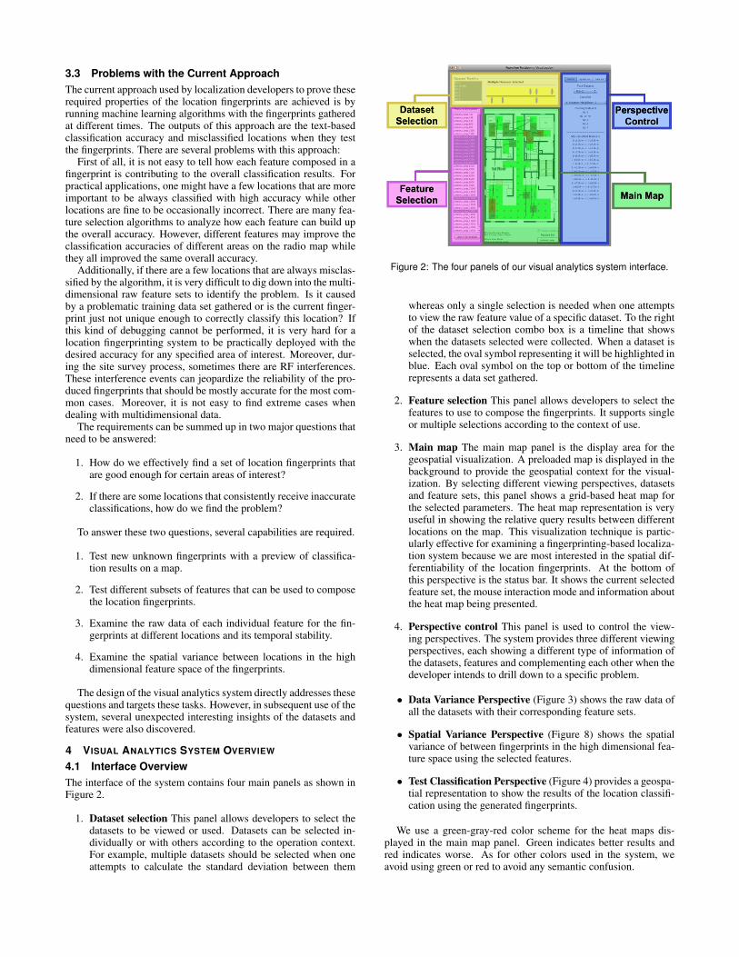
To illustrate use of this visual analytics system, we present an actualanalysis scenario we conducted using the PLP data. From our pre-vious research, we knew the original feature values (the raw signaldata) from the power line is useful for localization. However, sincethe original data was real valued, it is sometimes more clustered inthe high dimensional feature space. As a result, when the locationfingerprints contains certain amount of noise in the signal, the clas-sification would be incorrect. Therefore, one of the researchers pro-posed to transform the features of the datasets from raw amplitudevalues into the relative ranks of raw amplitude values as illustratedin Table 1. Using the ranking of the original feature values will cre-ate a unified spacing in between the them for each block. In theory,this approach can be more robust to noise because the real valuesare dynamically ranged and rounded up into a ranking form. Ourtask is to see if the PLP ranking version is better than the originalPLP system.

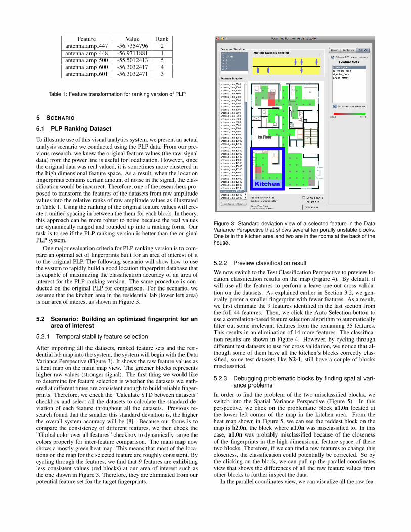
One major evaluation criteria for PLP ranking version is to com-pare an optimal set of fingerprints built for an area of interest of itto the original PLP. The following scenario will show how to usethe system to rapidly build a good location fingerprint database thatis capable of maximizing the classification accuracy of an area ofinterest for the PLP ranking version. The same procedure is con-ducted on the original PLP for comparison. For the scenario, weassume that the kitchen area in the residential lab (lower left area)is our area of interest as shown in Figure 3.

5.2 Scenario: Building an optimized fingerprint for anarea of interest

5.2.1 Temporal stability feature selection

After importing all the datasets, ranked feature sets and the resi-dential lab map into the system, the system will begin with the DataVariance Perspective (Figure 3). It shows the raw feature values asa heat map on the main map view. The greener blocks representshigher raw values (stronger signal). The first thing we would liketo determine for feature selection is whether the datasets we gath-ered at different times are consistent enough to build reliable finger-prints. Therefore, we check the ”Calculate STD between datasets”checkbox and select all the datasets to calculate the standard de-viation of each feature throughout all the datasets. Previous re-search found that the smaller this standard deviation is, the higherthe overall system accuracy will be [8]. Because our focus is tocompare the consistency of different features, we then check the”Global color over all features” checkbox to dynamically range thecolors properly for inter-feature comparison. The main map nowshows a mostly green heat map. This means that most of the loca-tions on the map for the selected feature are roughly consistent. Bycycling through the features, we find that 9 features are exhibitingless consistent values (red blocks) at our area of interest such asthe one shown in Figure 3. Therefore, they are eliminated from ourpotential feature set for the target fingerprints.

Figure 3: Standard deviation view of a selected feature in the DataVariance Perspective that shows several temporally unstable blocks.One is in the kitchen area and two are in the rooms at the back of thehouse.

5.2.2 Preview classification resultWe now switch to the Test Classification Perspective to preview lo-cation classification results on the map (Figure 4). By default, itwill use all the features to perform a leave-one-out cross valida-tion on the datasets. As explained earlier in Section 3.2, we gen-erally prefer a smaller fingerprint with fewer features. As a result,we first eliminate the 9 features identified in the last section fromthe full 44 features. Then, we click the Auto Selection button touse a correlation-based feature selection algorithm to automaticallyfilter out some irrelevant features from the remaining 35 features.This results in an elimination of 14 more features. The classifica-tion results are shown in Figure 4. However, by cycling throughdifferent test datasets to use for cross validation, we notice that al-though some of them have all the kitchen’s blocks correctly clas-sified, some test datasets like N2-1, still have a couple of blocksmisclassified.

5.2.3 Debugging problematic blocks by finding spatial vari-ance problems

In order to find the problem of the two misclassified blocks, weswitch into the Spatial Variance Perspective (Figure 5). In thisperspective, we click on the problematic block a1.0n located atthe lower left corner of the map in the kitchen area. From theheat map shown in Figure 5, we can see the reddest block on themap is b2.0n, the block where a1.0n was misclassified to. In thiscase, a1.0n was probably misclassified because of the closenessof the fingerprints in the high dimensional feature space of thesetwo blocks. Therefore, if we can find a few features to change thiscloseness, the classification could potentially be corrected. So bythe clicking on the block, we can pull up the parallel coordinatesview that shows the differences of all the raw feature values fromother blocks to further inspect the data.

In the parallel coordinates view, we can visualize all the raw fea-

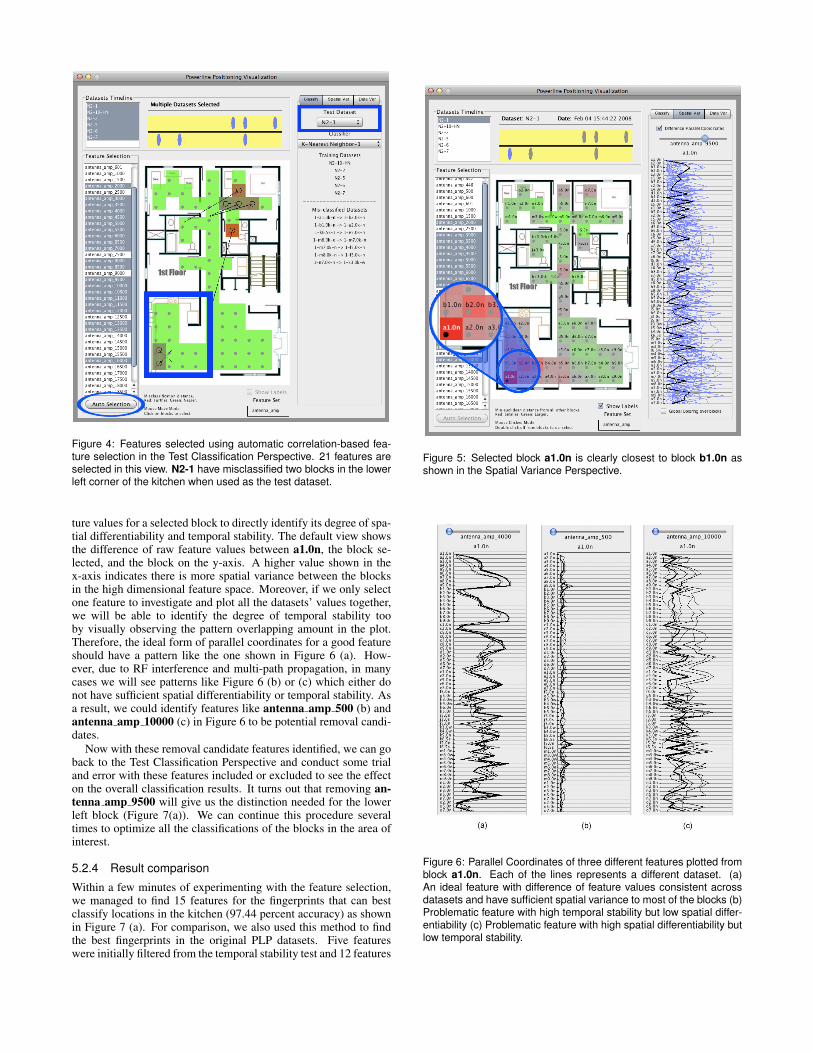
Figure 4: Features selected using automatic correlation-based fea-ture selection in the Test Classification Perspective. 21 features areselected in this view. N2-1 have misclassified two blocks in the lowerleft corner of the kitchen when used as the test dataset.

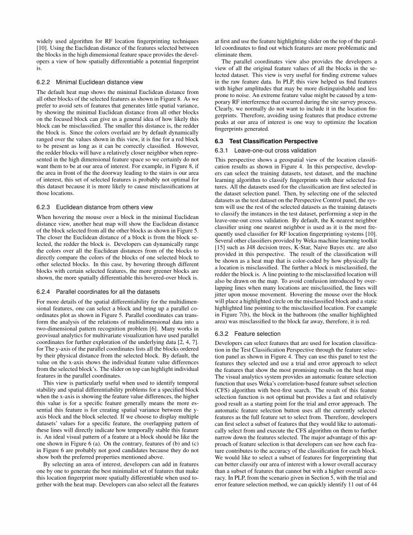
ture values for a selected block to directly identify its degree of spa-tial differentiability and temporal stability. The default view showsthe difference of raw feature values between a1.0n, the block se-lected, and the block on the y-axis. A higher value shown in thex-axis indicates there is more spatial variance between the blocksin the high dimensional feature space. Moreover, if we only selectone feature to investigate and plot all the datasets’ values together,we will be able to identify the degree of temporal stability tooby visually observing the pattern overlapping amount in the plot.Therefore, the ideal form of parallel coordinates for a good featureshould have a pattern like the one shown in Figure 6 (a). How-ever, due to RF interference and multi-path propagation, in manycases we will see patterns like Figure 6 (b) or (c) which either donot have sufficient spatial differentiability or temporal stability. Asa result, we could identify features like antenna amp 500 (b) andantenna amp 10000 (c) in Figure 6 to be potential removal candi-dates.

Now with these removal candidate features identified, we can goback to the Test Classification Perspective and conduct some trialand error with these features included or excluded to see the effecton the overall classification results. It turns out that removing an-tenna amp 9500 will give us the distinction needed for the lowerleft block (Figure 7(a)). We can continue this procedure severaltimes to optimize all the classifications of the blocks in the area ofinterest.

5.2.4 Result comparison

Within a few minutes of experimenting with the feature selection,we managed to find 15 features for the fingerprints that can bestclassify locations in the kitchen (97.44 percent accuracy) as shownin Figure 7 (a). For comparison, we also used this method to findthe best fingerprints in the original PLP datasets. Five featureswere initially filtered from the temporal stability test and 12 features

Figure 5: Selected block a1.0n is clearly closest to block b1.0n asshown in the Spatial Variance Perspective.

Figure 6: Parallel Coordinates of three different features plotted fromblock a1.0n. Each of the lines represents a different dataset. (a)An ideal feature with difference of feature values consistent acrossdatasets and have sufficient spatial variance to most of the blocks (b)Problematic feature with high temporal stability but low spatial differ-entiability (c) Problematic feature with high spatial differentiability butlow temporal stability.

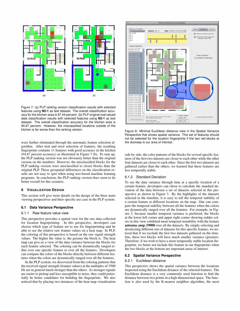
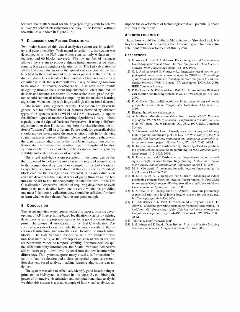
Figure 7: (a) PLP ranking version classification results with selectedfeatures using N2-1 as test dataset. The overall classification accu-racy for the kitchen area is 97.44 percent. (b) PLP original real valueddata classification results with selected features using N2-1 as testdataset. The overall classification accuracy for the kitchen area is94.87 percent. However, the misclassified locations outside of thekitchen is far worse than the ranking version.

were further eliminated through the automatic feature selection al-gorithm. After trial and error selection of features, the resultingfingerprints contains 11 features with good accuracy in the kitchen(94.87 percent accuracy) as illustrated in Figure 7 (b). To sum up,the PLP ranking version was not obviously better than the originalversion on the numbers. However, the misclassified blocks for thePLP ranking version were misclassified to closer blocks than theoriginal PLP. These geospatial differences on the classification re-sults are not easy to spot when using text-based machine learningprograms. In conclusion, the PLP ranking version does seem to dobetter overall for this scenario.

6 VISUALIZATION DESIGN

This section will give more details on the design of the three mainviewing perspectives and their specific use case in the PLP system.

6.1 Data Variance Perspective

6.1.1 Raw feature value view

This perspective provides a spatial view for the raw data collectedfor location fingerprinting. In this perspective, developers canchoose which type of feature set to use for fingerprinting and beable to see the relative raw feature values on a heat map. In PLP,the coloring of this perspective is based on the raw signal strengthvalues. The higher the value is, the greener the block is. The heatmap can give us a view of the data variance between the blocks foreach feature selected. The coloring can be dynamically ranged ei-ther over one specific feature or over all the features. Developerscan compare the colors of the blocks directly between different fea-tures when the colors are dynamically ranged over all the features.

In the PLP system, we discovered from the coloring patterns thatthe received signal strength (feature values) at the multiples of 3500Hz are in general much stronger than the others. As stronger signalsare easier to pickup and less susceptible to noise, they could poten-tially be better candidates for building the fingerprints. We alsonoticed that by placing two instances of the heat map visualization

Figure 8: Minimal Euclidean distance view in the Spatial VariancePerspective that shows spatial variance. This set of features shouldnot be selected for the location fingerprints if the two red blocks atthe doorway is our area of interest.

side by side, the color patterns of the blocks for several specific fea-tures of the first two datasets are closer to each other while the otherfour datasets are closer to each other. Since the first two datasets aregathered earlier than the others, we learned that these features areless temporally stable.

6.1.2 Standard DeviationTo see the data variance through time at a specific location of acertain feature, developers can chose to calculate the standard de-viation of the data between a set of datasets selected in this per-spective as shown in Figure 3. By the highlights of the datasetsselected in the timeline, it is easy to tell the temporal stability ofa certain feature at different locations on the map. One can com-pare the temporal stability between all the features when the colorsare dynamically ranged over all the features. For example, in Fig-ure 3, because smaller temporal variance is preferred, the blocksat the lower left corner and upper right corner showing redder col-ors in this view exhibited more temporal instability with the featureantenna amp 19000 over all the datasets. By simply selecting anddeselecting different sets of datasets for this specific feature, we no-ticed that if we exclude the first two datasets gathered on the time-line, these two blocks will have much smaller variance (greener).Therefore, if we wish to have a more temporally stable location fin-gerprint, we better not include this feature in our fingerprints whenthe two blocks at the bottom are important areas of interest.

6.2 Spatial Variance Perspective6.2.1 Euclidean distanceThis perspective shows the spatial variance between the locationsinspected using the Euclidean distance of the selected features. TheEuclidean distance is a very commonly used function to find thedistance between two points in a high dimensional space. The func-tion is also used by the K-nearest neighbor algorithm, the most

widely used algorithm for RF location fingerprinting techniques[10]. Using the Euclidean distance of the features selected betweenthe blocks in the high dimensional feature space provides the devel-opers a view of how spatially differentiable a potential fingerprintis.

6.2.2 Minimal Euclidean distance view

The default heat map shows the minimal Euclidean distance fromall other blocks of the selected features as shown in Figure 8. As weprefer to avoid sets of features that generates little spatial variance,by showing the minimal Euclidean distance from all other blockson the focused block can give us a general idea of how likely thisblock can be misclassified. The smaller this distance is, the redderthe block is. Since the colors overlaid are by default dynamicallyranged over the values shown in this view, it is fine for a red blockto be present as long as it can be correctly classified. However,the redder blocks will have a relatively closer neighbor when repre-sented in the high dimensional feature space so we certainly do notwant them to be at our area of interest. For example, in Figure 8, ifthe area in front of the the doorway leading to the stairs is our areaof interest, this set of selected features is probably not optimal forthis dataset because it is more likely to cause misclassifications atthose locations.

6.2.3 Euclidean distance from others view

When hovering the mouse over a block in the minimal Euclideandistance view, another heat map will show the Euclidean distanceof the block selected from all the other blocks as shown in Figure 5.The closer the Euclidean distance of a block is from the block se-lected, the redder the block is. Developers can dynamically rangethe colors over all the Euclidean distances from of the blocks todirectly compare the colors of the blocks of one selected block toother selected blocks. In this case, by hovering through differentblocks with certain selected features, the more greener blocks areshown, the more spatially differentiable this hovered-over block is.

6.2.4 Parallel coordinates for all the datasets

For more details of the spatial differentiability for the multidimen-sional features, one can select a block and bring up a parallel co-ordinates plot as shown in Figure 5. Parallel coordinates can trans-form the analysis of the relations of multidimensional data into atwo-dimensional pattern recognition problem [6]. Many works ingeovisual analytics for multivariate visualization have used parallelcoordinates for further exploration of the underlying data [2, 4, 7].for The y-axis of the parallel coordinates lists all the blocks orderedby their physical distance from the selected block. By default, thevalue on the x-axis shows the individual feature value differencesfrom the selected block’s. The slider on top can highlight individualfeatures in the parallel coordinates.

This view is particularly useful when used to identify temporalstability and spatial differentiability problems for a specified blockwhen the x-axis is showing the feature value differences, the higherthis value is for a specific feature generally means the more es-sential this feature is for creating spatial variance between the y-axis block and the block selected. If we choose to display multipledatasets’ values for a specific feature, the overlapping pattern ofthese lines will directly indicate how temporally stable this featureis. An ideal visual pattern of a feature at a block should be like theone shown in Figure 6 (a). On the contrary, features of (b) and (c)in Figure 6 are probably not good candidates because they do notshow both the preferred properties mentioned above.

By selecting an area of interest, developers can add in featuresone by one to generate the best minimalist set of features that makethis location fingerprint more spatially differentiable when used to-gether with the heat map. Developers can also select all the features

at first and use the feature highlighting slider on the top of the paral-lel coordinates to find out which features are more problematic andeliminate them.

The parallel coordinates view also provides the developers aview of all the original feature values of all the blocks in the se-lected dataset. This view is very useful for finding extreme valuesin the raw feature data. In PLP, this view helped us find featureswith higher amplitudes that may be more distinguishable and lessprone to noise. An extreme feature value might be caused by a tem-porary RF interference that occurred during the site survey process.Clearly, we normally do not want to include it in the location fin-gerprints. Therefore, avoiding using features that produce extremepeaks at our area of interest is one way to optimize the locationfingerprints generated.

6.3 Test Classification Perspective6.3.1 Leave-one-out cross validationThis perspective shows a geospatial view of the location classifi-cation results as shown in Figure 4. In this perspective, develop-ers can select the training datasets, test dataset, and the machinelearning algorithm to classify fingerprints with their selected fea-tures. All the datasets used for the classification are first selected inthe dataset selection panel. Then, by selecting one of the selecteddatasets as the test dataset on the Perspective Control panel, the sys-tem will use the rest of the selected datasets as the training datasetsto classify the instances in the test dataset, performing a step in theleave-one-out cross validation. By default, the K-nearest neighborclassifier using one nearest neighbor is used as it is the most fre-quently used classifier for RF location fingerprinting systems [10].Several other classifiers provided by Weka machine learning toolkit[15] such as J48 decision trees, K-Star, Naive Bayes etc. are alsoprovided in this perspective. The result of the classification willbe shown as a heat map that is color-coded by how physically fara location is misclassified. The further a block is misclassified, theredder the block is. A line pointing to the misclassified location willalso be drawn on the map. To avoid confusion introduced by over-lapping lines when many locations are misclassified, the lines willjitter upon mouse movement. Hovering the mouse over the blockwill place a highlighted circle on the misclassified block and a statichighlighted line pointing to the misclassified location. For examplein Figure 7(b), the block in the bathroom (the smaller highlightedarea) was misclassified to the block far away, therefore, it is red.

6.3.2 Feature selectionDevelopers can select features that are used for location classifica-tion in the Test Classification Perspective through the feature selec-tion panel as shown in Figure 4. They can use this panel to test thefeatures they selected and use a trial and error approach to selectthe features that show the most promising results on the heat map.The visual analytics system provides an automatic feature selectionfunction that uses Weka’s correlation-based feature subset selection(CFS) algorithm with best-first search. The result of this featureselection function is not optimal but provides a fast and relativelygood result as a starting point for the trial and error approach. Theautomatic feature selection button uses all the currently selectedfeatures as the full feature set to select from. Therefore, developerscan first select a subset of features that they would like to automati-cally select from and execute the CFS algorithm on them to furthernarrow down the features selected. The major advantage of this ap-proach of feature selection is that developers can see how each fea-ture contributes to the accuracy of the classification for each block.We would like to select a subset of features for fingerprinting thatcan better classify our area of interest with a lower overall accuracythan a subset of features that cannot but with a higher overall accu-racy. In PLP, from the scenario given in Section 5, with the trial anderror feature selection method, we can quickly identify 11 out of 44

features that matters most for the fingerprinting system to achievean over 90 percent classification accuracy in the kitchen within afew minutes as shown in Figure 7 (b).

7 DISCUSSION AND FUTURE DIRECTIONS

Two major issues of this visual analytics system are its scalabil-ity and generalizability. With regard to scalability, the system wasdeveloped with the PLP data which consists only 6 datasets, 44features, and 66 blocks surveyed. The low number of instancesallowed the system to produce almost instantaneous results whenrunning K-nearest neighbor classifier on it. The fast calculation ofall the Euclidean distances in the spatial variance perspective alsobenefited by the small amount of instances present. If there are hun-dreds of datasets, each dataset has hundreds of features, or a slowerclassifier is used, the system will very likely be running too slowto be usable. Moreover, developers will also have more troublenavigating through the current implementation when hundreds ofdatasets and features are shown. A more scalable design of the sys-tem should support distributed computing for the machine learningalgorithms when dealing with large and high dimensional datasets.

The second issue is generalizability. The system design can begeneralized for different kinds of features provided by differenttypes of RF systems such as Wi-Fi and GSM. However, its supportfor different types of machine learning algorithms is very limited,especially on the Spatial Variance Perspective. If using a differentalgorithm other than K-nearest neighbors for classification, the no-tion of ”distance” will be different. Future work for generalizabilityshould explore having more distance functions built in for showingspatial variances between different blocks and coupling them withthe classification algorithm in the Test Classification Perspective.Systematic user evaluations on other fingerprinting-based locationsystems can be further conducted to better understand the general-izability and scalability issues of our system.

The visual analytics system presented in this paper can be fur-ther improved by delegating more currently required manual workto the computational system. For example, in the Data VariancePerspective, a color-coded feature list that can show the ”reddest”block color or the average color presented in its individual viewcan save developers the manual work of going through all the fea-tures in the list to find the temporally unstable features. In the TestClassification Perspective, instead of requiring developers to cyclethrough the more detailed leave-one-out cross validation, providingone meta 3-fold cross-validation view should be sufficient for themto learn whether the selected features are good enough.

8 CONCLUSION

The visual analytics system presented in this paper aids in the devel-opment of RF fingerprinting-based localization systems by helpingdevelopers select appropriate features for a good location finger-print. The geospatial visualization in the Test Classification Per-spective gives developers not only the accuracy results of the lo-cation classification, but also the exact location of misclassifiedblocks. The Data Variance Perspective with the standard devia-tion heat map can give the developers an idea of which featuresare better with respect to temporal stability. For more detailed spa-tial differentiability information, the Spatial Variance Perspectiveallows users to go down level by level into the raw feature valuedifferences. This system supports many visual aids for location fin-gerprint feature selection and a clear geospatial output representa-tion that text-based analytic machine learning algorithms can notdeliver.

The system was able to effectively identify good location finger-prints on the PLP system as shown in this paper. By combining thepower of interactive visualization and computational data analysis,we think this system is a great example of how visual analytics can

support the development of technologies that will potentially shapeour lives in the future.

ACKNOWLEDGEMENTS

The authors would like to thank Mario Romero, Shwetak Patel, Jef-frey Hightower and the Georgia Tech Ubicomp group for their valu-able input to the development of this system.

REFERENCES

[1] G. Andrienko and N. Andrienko. Data mining with c4.5 and interac-tive cartographic visualization. In User Interfaces to Data IntensiveSystems, 1999. Proceedings, pages 162–165, 1999.

[2] G. L. Andrienko and N. V. Andrienko. Interactive visual tools to sup-port spatial multicriteria decision making. In UIDIS ’01: Proceedingsof the Second International Workshop on User Interfaces to Data In-tensive Systems (UIDIS’01), page 127, Washington, DC, USA, 2001.IEEE Computer Society.

[3] P. Bahl and V. N. Padmanabhan. RADAR: An in-building RF-baseduser location and tracking system. In INFOCOM (2), pages 775–784,2000.

[4] R. M. Edsall. The parallel coordinate plot in action: design and use forgeographic visualization. Comput. Stat. Data Anal., 43(4):605–619,2003.

[5] Ekahau. http://www.ekahau.com/.[6] A. Inselberg. Multidimensional detective. In INFOVIS ’97: Proceed-

ings of the 1997 IEEE Symposium on Information Visualization (In-foVis ’97), page 100, Washington, DC, USA, 1997. IEEE ComputerSociety.

[7] S. Johansson and M. Jern. Geoanalytics visual inquiry and filteringtools in parallel coordinates plots. In GIS ’07: Proceedings of the 15thannual ACM international symposium on Advances in geographic in-formation systems, pages 1–8, New York, NY, USA, 2007. ACM.

[8] K. Kaemarungsi and P. Krishnamurthy. Modeling of indoor position-ing systems based on location fingerprinting. In IEEE Infocom, HongKong, pages 1012–1022, 2004.

[9] K. Kaemarungsi and P. Krishnamurthy. Properties of indoor receivedsignal strength for wlan location fingerprinting. Mobile and Ubiqui-tous Systems, Annual International Conference on, 0:14–23, 2004.

[10] M. B. Kjærgaard. A taxonomy for radio location fingerprinting. InLoCA, pages 139–156, 2007.

[11] B. Li, J. Salter, A. G. Dempster, and C. Rizos. Modeling of indoorpositioning systems based on location fingerprinting. In First IEEEInternational Conference on Wireless Broadband and Ultra WidebandCommunications, Sydney, Australia, 2006.

[12] S. N. Patel, K. N. Truong, and G. D. Abowd. Powerline positioning:A practical sub-room-level indoor location system for domestic use.In Ubicomp, pages 441–458, 2006.

[13] E. P. Stuntebeck, S. N. Patel, T. Robertson, M. S. Reynolds, and G. D.Abowd. Wideband powerline positioning for indoor localization. InUbiComp ’08: Proceedings of the 10th international conference onUbiquitous computing, pages 94–103, New York, NY, USA, 2008.ACM.

[14] Tektronix. http://www.tek.com/.[15] I. H. Witten and E. Frank. Data Mining: Practical Machine Learning

Tools and Techniques. Morgan Kaufmann, 2 edition, 2005.