Embed Size (px)
Citation preview
AIMS Energy, 5(6): 887-911.
DOI: 10.3934/energy.2017.6.887
Received: 08 September 2017
Accepted: 05 November 2017
Published: 13 November 2017
http://www.aimspress.com/journal/energy
Research article
A virtual power plant model for time-driven power flow calculations
Gerardo Guerra and Juan A. Martinez Velasco *
Departament d’Enginyeria Electrica, Universitat Politecnica de Catalunya, Av. Diagonal 647, 08028
Barcelona, Spain
* Correspondence: Email: [email protected]; Tel: +3-493-401-6725.
Abstract: This paper presents the implementation of a custom-made virtual power plant model in
OpenDSS. The goal is to develop a model adequate for time-driven power flow calculations in
distribution systems. The virtual power plant is modeled as the aggregation of renewable generation
and energy storage connected to the distribution system through an inverter. The implemented
operation mode allows the virtual power plant to act as a single dispatchable generation unit. The
case studies presented in the paper demonstrate that the model behaves according to the specified
control algorithm and show how it can be incorporated into the solution scheme of a general parallel
genetic algorithm in order to obtain the optimal day-ahead dispatch. Simulation results exhibit a clear
benefit from the deployment of a virtual power plant when compared to distributed generation based
only on renewable intermittent generation.
Keywords: distribution system; energy resource; energy storage system; OpenDSS; photovoltaic
generation; power flow; virtual power plant; wind generation
1. Introduction
The increasing penetration of renewable generation has been motivated by the necessity of
reducing the current dependence on non-renewable energy sources. Solar and wind power systems
are two of the most widespread forms of electricity generation based on renewable energy resources.
The modular nature of these technologies makes them a suitable option for the deployment of small
scale generation connected at distribution level, namely as distributed generation (DG).
DG can be used for supporting voltage, reducing losses, providing backup power and ancillary
services, or deferring distribution system upgrade [1,2,3]. However, the intermittent nature of some
888
AIMS Energy Volume 5, Issue 6, 887-911.
renewable resources (e.g. solar and wind) complicates their integration into the grid as they cannot be
properly dispatched. In general, renewable generation is permitted to produce as much power as the
resource availability allows; this approach limits the integration of renewable DG since unacceptable
operating conditions may appear under large penetration scenarios (e.g. system voltages above
accepted limits).
Energy storage (ES) capabilities can be used to improve network operation and compensate the
intermittency of renewable generation [4–7]. Through the aggregation of renewable DG and ES, it is
possible to constitute an entity, known as a virtual power plant (VPP), which can operate as a single
dispatchable power plant [8,9]. As part of a VPP, ES can be charged when there is a generation
excess and provide support to meet the dispatched power when DG generation decreases.
This paper presents the implementation of a custom-made VPP model for power flow
calculations in OpenDSS [10]. The objective is to present a model based on the storage object
available in OpenDSS, adequate for distribution system studies and quasi-static (time-driven)
simulations. The VPP model has been compiled within the OpenDSS COM DLL and can be used in
simulations driven from other software platforms, e.g. MATLAB.
The paper is organized as follows. Section 2 details the configuration and operation of the
implemented model. A case study aimed at demonstrating the model behavior is presented in
Section 3. The optimization of the hourly day-ahead dispatch using a genetic algorithm (GA) is
explored in Section 4. The main conclusions drawn from the paper, as well as future work, are
summarized in Section 5.
2. VPP Model for Power Flow Calculations
2.1. VPP definition
A VPP can be defined as a flexible representation of a portfolio of distributed energy
resources (DERs), in which a single operating profile can be created from a composite of parameters
characterizing each DER [11]. Through the aggregation of DERs it is possible for the VPP to operate
as a system-connected power plant and have access to wholesale energy markets and provide support
services for the transmission system management.
VPPs can be classified as commercial VPP (CVPP) or technical VPP (TVPP) [11]. A number of
DERs can participate in the energy market as a single CVPP, while the TVPP models the
characteristics of a system that contains an aggregation of DERs, and acts as a single power plant.
The CVPP can represent resources from different locations, whereas all DERs in a TVPP belong to
the same geographical location.
The main elements that compose a VPP are: (i) energy production units, (ii) energy storage
units, and (iii) flexible loads [12]. The VPP must exert control over the different elements in order to
coordinate and optimize their operation. VPP control is conducted via a communication system that
connects all the DERs in the VPP [8,13].
A VPP can also be defined as an aggregation of power production from a group of grid-
connected DERs operated by a centralized controller [9]. According to this definition, the
combination of DG and ES with a coordinated control can also be considered as a VPP, since it
allows them to operate as a single dispatchable power plant. Although exporting energy to the
transmission system is still possible (by reversing the power flow through the substation transformer),
889
AIMS Energy Volume 5, Issue 6, 887-911.
the VPP’s main task will be to provide support to the distribution network as dispatchable DG. The
model presented in this section corresponds to this definition of VPP and only considers the
aggregation of energy storage and renewable generation, either photovoltaic (PV) or wind.
2.2. VPP configuration and components
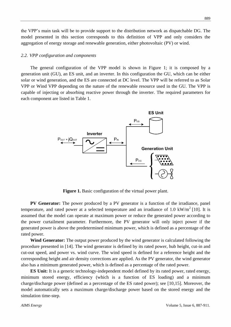
The general configuration of the VPP model is shown in Figure 1; it is composed by a
generation unit (GU), an ES unit, and an inverter. In this configuration the GU, which can be either
solar or wind generation, and the ES are connected at DC level. The VPP will be referred to as Solar
VPP or Wind VPP depending on the nature of the renewable resource used in the GU. The VPP is
capable of injecting or absorbing reactive power through the inverter. The required parameters for
each component are listed in Table 1.
Figure 1. Basic configuration of the virtual power plant.
PV Generator: The power produced by a PV generator is a function of the irradiance, panel
temperature, and rated power at a selected temperature and an irradiance of 1.0 kW/m2
[10]. It is
assumed that the model can operate at maximum power or reduce the generated power according to
the power curtailment parameter. Furthermore, the PV generator will only inject power if the
generated power is above the predetermined minimum power, which is defined as a percentage of the
rated power.
Wind Generator: The output power produced by the wind generator is calculated following the
procedure presented in [14]. The wind generator is defined by its rated power, hub height, cut-in and
cut-out speed, and power vs. wind curve. The wind speed is defined for a reference height and the
corresponding height and air density corrections are applied. As the PV generator, the wind generator
also has a minimum generated power, which is defined as a percentage of the rated power.
ES Unit: It is a generic technology-independent model defined by its rated power, rated energy,
minimum stored energy, efficiency (which is a function of ES loading) and a minimum
charge/discharge power (defined as a percentage of the ES rated power); see [10,15]. Moreover, the
model automatically sets a maximum charge/discharge power based on the stored energy and the
simulation time-step.
890
AIMS Energy Volume 5, Issue 6, 887-911.
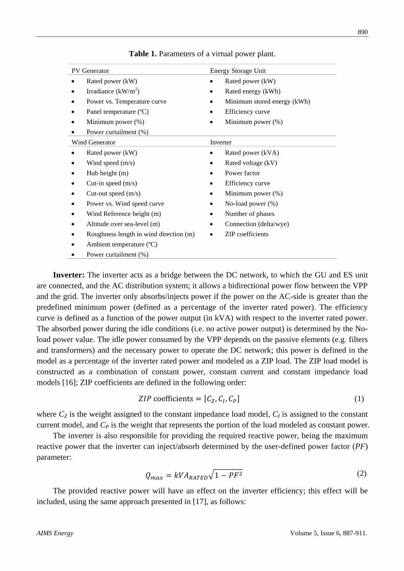
Table 1. Parameters of a virtual power plant.
PV Generator Energy Storage Unit
Rated power (kW) Rated power (kW)
Irradiance (kW/m2) Rated energy (kWh)
Power vs. Temperature curve Minimum stored energy (kWh)
Panel temperature (ºC) Efficiency curve
Minimum power (%) Minimum power (%)
Power curtailment (%)
Wind Generator Inverter
Rated power (kW) Rated power (kVA)
Wind speed (m/s) Rated voltage (kV)
Hub height (m) Power factor
Cut-in speed (m/s) Efficiency curve
Cut-out speed (m/s) Minimum power (%)
Power vs. Wind speed curve No-load power (%)
Wind Reference height (m) Number of phases
Altitude over sea-level (m) Connection (delta/wye)
Roughness length in wind direction (m) ZIP coefficients
Ambient temperature (ºC)
Power curtailment (%)
Inverter: The inverter acts as a bridge between the DC network, to which the GU and ES unit
are connected, and the AC distribution system; it allows a bidirectional power flow between the VPP
and the grid. The inverter only absorbs/injects power if the power on the AC-side is greater than the
predefined minimum power (defined as a percentage of the inverter rated power). The efficiency
curve is defined as a function of the power output (in kVA) with respect to the inverter rated power.
The absorbed power during the idle conditions (i.e. no active power output) is determined by the No-
load power value. The idle power consumed by the VPP depends on the passive elements (e.g. filters
and transformers) and the necessary power to operate the DC network; this power is defined in the
model as a percentage of the inverter rated power and modeled as a ZIP load. The ZIP load model is
constructed as a combination of constant power, constant current and constant impedance load
models [16]; ZIP coefficients are defined in the following order:
(1)
where CZ is the weight assigned to the constant impedance load model, CI is assigned to the constant
current model, and CP is the weight that represents the portion of the load modeled as constant power.
The inverter is also responsible for providing the required reactive power, being the maximum
reactive power that the inverter can inject/absorb determined by the user-defined power factor (PF)
parameter:
(2)
The provided reactive power will have an effect on the inverter efficiency; this effect will be
included, using the same approach presented in [17], as follows:
891
AIMS Energy Volume 5, Issue 6, 887-911.
(3)
(4)
(5)
where Qmax is the maximum reactive power and kVARATED is the inverter rated power. is the
efficiency curve for any load level, s, and any output power factor, pf, f (s) is the efficiency curve for
a unity power factor, which depends on the load level (measured at the AC-side), and α is a scale
factor that depends on the power factor.
2.3. VPP operation
The VPP model has been developed for time-driven simulations and takes advantage of
OpenDSS built-in capabilities (i.e. loadshapes, linear interpolation, complex number operations, etc.).
Two operation modes have been defined for the VPP: (i) Follow mode; (ii) Dispatch mode.
2.3.1. Follow operation mode
Under this operation mode the ES unit and the GU behave according to the curve shapes
assigned to each component. The PV generator requires curves describing the solar irradiance and
panel temperature for the evaluation period, while the wind generator follows the curves that define
the wind speed (measured at a reference height) and the ambient temperature. On the other hand, ES
unit operates according to a curve that defines the charge and discharge states, as well as the
absorbed and injected power. The reactive power provided by the inverter is equal to the maximum
reactive power times the corresponding multiplier stored in a user-defined curve shape.
The total VPP power output is not controlled and depends on the power resulting from the
interaction between the GU and the ES unit. The model follows the same convention as the
OpenDSS Storage object: Negative values correspond to power absorption, while power injection is
defined by positive values. The VPP powers are calculated according to the following equations (see
Figure 1):
(6)
(7)
where PDG is the power produced by the GU, PES is the power provided by the ES unit, PIN is the
power measured at the inverter DC-side, POUT is the active power measured at the inverter AC-side,
and η is the inverter efficiency, calculated according to Equations (3) through (5).
892
AIMS Energy Volume 5, Issue 6, 887-911.
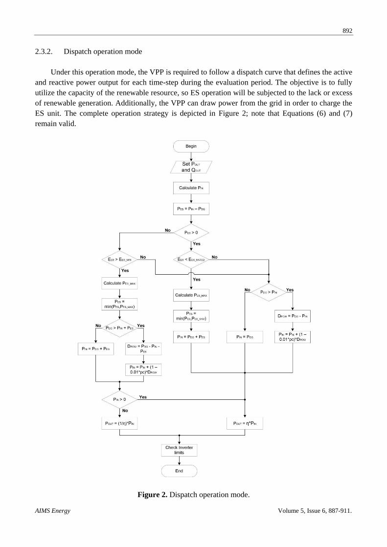
2.3.2. Dispatch operation mode
Under this operation mode, the VPP is required to follow a dispatch curve that defines the active
and reactive power output for each time-step during the evaluation period. The objective is to fully
utilize the capacity of the renewable resource, so ES operation will be subjected to the lack or excess
of renewable generation. Additionally, the VPP can draw power from the grid in order to charge the
ES unit. The complete operation strategy is depicted in Figure 2; note that Equations (6) and (7)
remain valid.
Figure 2. Dispatch operation mode.
893
AIMS Energy Volume 5, Issue 6, 887-911.
In Figure 2 EES is the current stored energy in the ES unit, EES_RATED is the ES rated energy,
EES_MIN is the minimum stored energy, PES_MAX is the maximum power the ES unit can absorb/inject
based on the current stored energy, and pc is the power curtailment parameter.
The following aspects must be taken into account for the Dispatch operation mode:
POUT is calculated as the inverter rated power times the corresponding multiplier stored in a
user-defined curve shape.
The reactive power provided by the inverter (QOUT) is equal to the maximum reactive power
times the corresponding multiplier stored in a user-defined curve shape.
PIN is calculated from Equation (7).
The power produced by the GU is defined by the curves describing the renewable
resource (irradiance or wind speed) and temperature (panel or ambient) for the evaluation period.
The ES unit main task is to compensate for the lack or excess of renewable generation. ES
power will be adjusted so PIN matches the power required to meet the VPP dispatch.
By defining a negative multiplier, the VPP can be forced to absorb active power, which will be
used to charge the ES unit with power coming from the distribution network.
VPP operation is meant to follow the power dispatch as accurately as possible; therefore,
renewable generation may be curtailed in order to prevent any deviation from the dispatched
power. For example, assume the ES unit is fully charged and the available power is greater than
the required power to meet the VPP dispatch; under this condition, the GU production will be
reduced in order to match the dispatched power. However, power curtailment is not a binary
decision, that is, the amount of power to be curtailed is defined by the power curtailment
parameter.
If the available power in the VPP (including ES and GU) is not enough to meet the dispatched
power, the VPP will export as much power as resource availability allows.
The VPP can enter an idle state under three conditions: (i) the dispatched active power is equal
to zero; (ii) the available power within the VPP is zero, which would make the VPP unable to
meet any dispatched power, and (iii) SOUT (the apparent power at the AC-side) is smaller than
the inverter minimum power. In idle state the VPP will only draw active power, determined by
the user-defined No-load parameter and ZIP coefficients.
The last step in the procedure verifies that SOUT is not greater than the inverter rated power; if so,
the model will adjust POUT, QOUT, PDG, and PES so the resulting SOUT is equal to the inverter
rated power. This function is also used under the Follow operation mode.
For a time-driven simulation, the procedure must be repeated for every time-step.
3. Simulation of the VPP Model Under Dispatch Operation Mode
3.1. Test system configuration and characteristics
This section is aimed at illustrating the behavior of the VPP model running under Dispatch
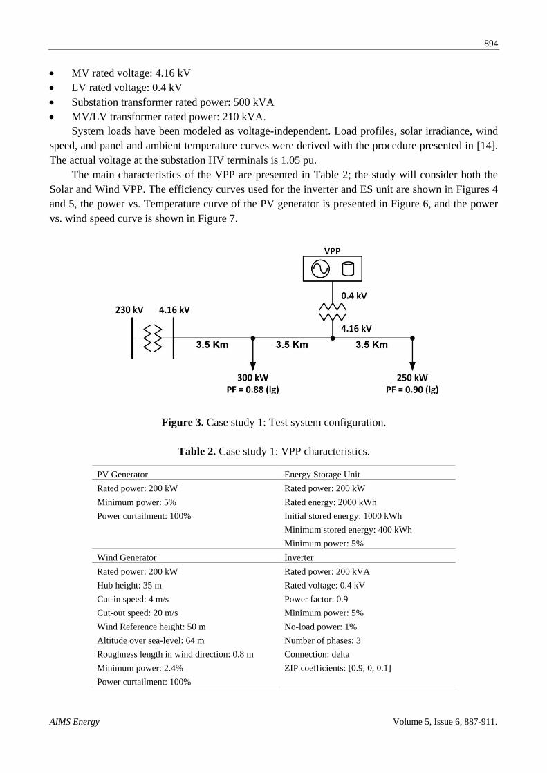
operation mode. Figure 3 shows the test system: it is a three-phase 60-Hz overhead system serving
two spot loads supplied from a HV/MV substation transformer. The VPP is connected to the MV
network through a distribution MV/LV transformer.
The main characteristics of the test system are as follows:
HV rated voltage: 230 kV
894
AIMS Energy Volume 5, Issue 6, 887-911.
MV rated voltage: 4.16 kV
LV rated voltage: 0.4 kV
Substation transformer rated power: 500 kVA
MV/LV transformer rated power: 210 kVA.
System loads have been modeled as voltage-independent. Load profiles, solar irradiance, wind
speed, and panel and ambient temperature curves were derived with the procedure presented in [14].
The actual voltage at the substation HV terminals is 1.05 pu.
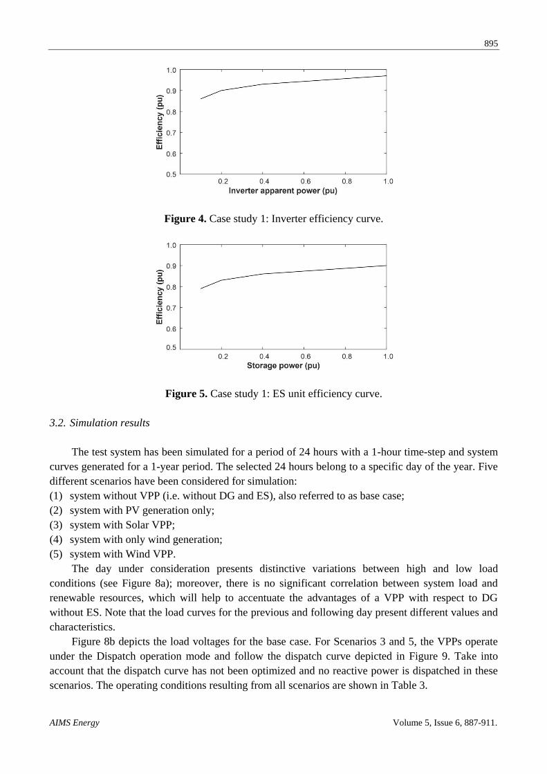
The main characteristics of the VPP are presented in Table 2; the study will consider both the
Solar and Wind VPP. The efficiency curves used for the inverter and ES unit are shown in Figures 4
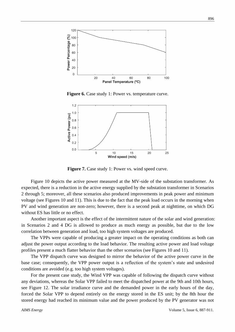
and 5, the power vs. Temperature curve of the PV generator is presented in Figure 6, and the power
vs. wind speed curve is shown in Figure 7.
Figure 3. Case study 1: Test system configuration.
Table 2. Case study 1: VPP characteristics.
PV Generator Energy Storage Unit
Rated power: 200 kW Rated power: 200 kW
Minimum power: 5% Rated energy: 2000 kWh
Power curtailment: 100% Initial stored energy: 1000 kWh
Minimum stored energy: 400 kWh
Minimum power: 5%
Wind Generator Inverter
Rated power: 200 kW Rated power: 200 kVA
Hub height: 35 m Rated voltage: 0.4 kV
Cut-in speed: 4 m/s Power factor: 0.9
Cut-out speed: 20 m/s Minimum power: 5%
Wind Reference height: 50 m No-load power: 1%
Altitude over sea-level: 64 m Number of phases: 3
Roughness length in wind direction: 0.8 m Connection: delta
Minimum power: 2.4% ZIP coefficients: [0.9, 0, 0.1]
Power curtailment: 100%
895
AIMS Energy Volume 5, Issue 6, 887-911.
Figure 4. Case study 1: Inverter efficiency curve.
Figure 5. Case study 1: ES unit efficiency curve.
3.2. Simulation results
The test system has been simulated for a period of 24 hours with a 1-hour time-step and system
curves generated for a 1-year period. The selected 24 hours belong to a specific day of the year. Five
different scenarios have been considered for simulation:
(1) system without VPP (i.e. without DG and ES), also referred to as base case;
(2) system with PV generation only;
(3) system with Solar VPP;
(4) system with only wind generation;
(5) system with Wind VPP.
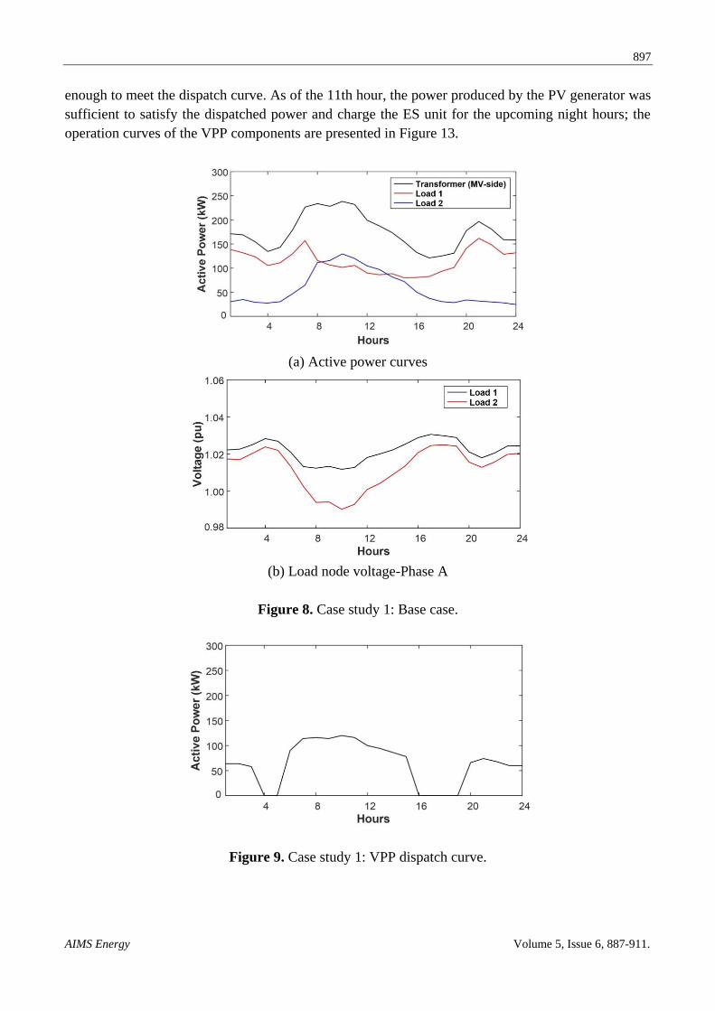
The day under consideration presents distinctive variations between high and low load
conditions (see Figure 8a); moreover, there is no significant correlation between system load and
renewable resources, which will help to accentuate the advantages of a VPP with respect to DG
without ES. Note that the load curves for the previous and following day present different values and
characteristics.
Figure 8b depicts the load voltages for the base case. For Scenarios 3 and 5, the VPPs operate
under the Dispatch operation mode and follow the dispatch curve depicted in Figure 9. Take into
account that the dispatch curve has not been optimized and no reactive power is dispatched in these
scenarios. The operating conditions resulting from all scenarios are shown in Table 3.
896
AIMS Energy Volume 5, Issue 6, 887-911.
Figure 6. Case study 1: Power vs. temperature curve.
Figure 7. Case study 1: Power vs. wind speed curve.
Figure 10 depicts the active power measured at the MV-side of the substation transformer. As
expected, there is a reduction in the active energy supplied by the substation transformer in Scenarios
2 through 5; moreover, all these scenarios also produced improvements in peak power and minimum
voltage (see Figures 10 and 11). This is due to the fact that the peak load occurs in the morning when
PV and wind generation are non-zero; however, there is a second peak at nighttime, on which DG
without ES has little or no effect.
Another important aspect is the effect of the intermittent nature of the solar and wind generation:
in Scenarios 2 and 4 DG is allowed to produce as much energy as possible, but due to the low
correlation between generation and load, too high system voltages are produced.
The VPPs were capable of producing a greater impact on the operating conditions as both can
adjust the power output according to the load behavior. The resulting active power and load voltage
profiles present a much flatter behavior than the other scenarios (see Figures 10 and 11).
The VPP dispatch curve was designed to mirror the behavior of the active power curve in the
base case; consequently, the VPP power output is a reflection of the system’s state and undesired
conditions are avoided (e.g. too high system voltages).
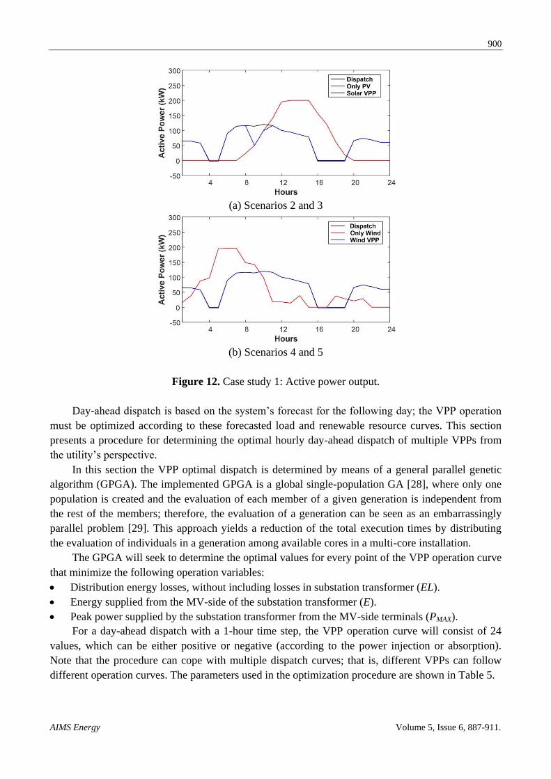
For the present case study, the Wind VPP was capable of following the dispatch curve without
any deviations, whereas the Solar VPP failed to meet the dispatched power at the 9th and 10th hours,
see Figure 12. The solar irradiance curve and the demanded power in the early hours of the day,
forced the Solar VPP to depend entirely on the energy stored in the ES unit; by the 8th hour the
stored energy had reached its minimum value and the power produced by the PV generator was not
897
AIMS Energy Volume 5, Issue 6, 887-911.
enough to meet the dispatch curve. As of the 11th hour, the power produced by the PV generator was
sufficient to satisfy the dispatched power and charge the ES unit for the upcoming night hours; the
operation curves of the VPP components are presented in Figure 13.
(a) Active power curves
(b) Load node voltage-Phase A
Figure 8. Case study 1: Base case.
Figure 9. Case study 1: VPP dispatch curve.
898
AIMS Energy Volume 5, Issue 6, 887-911.
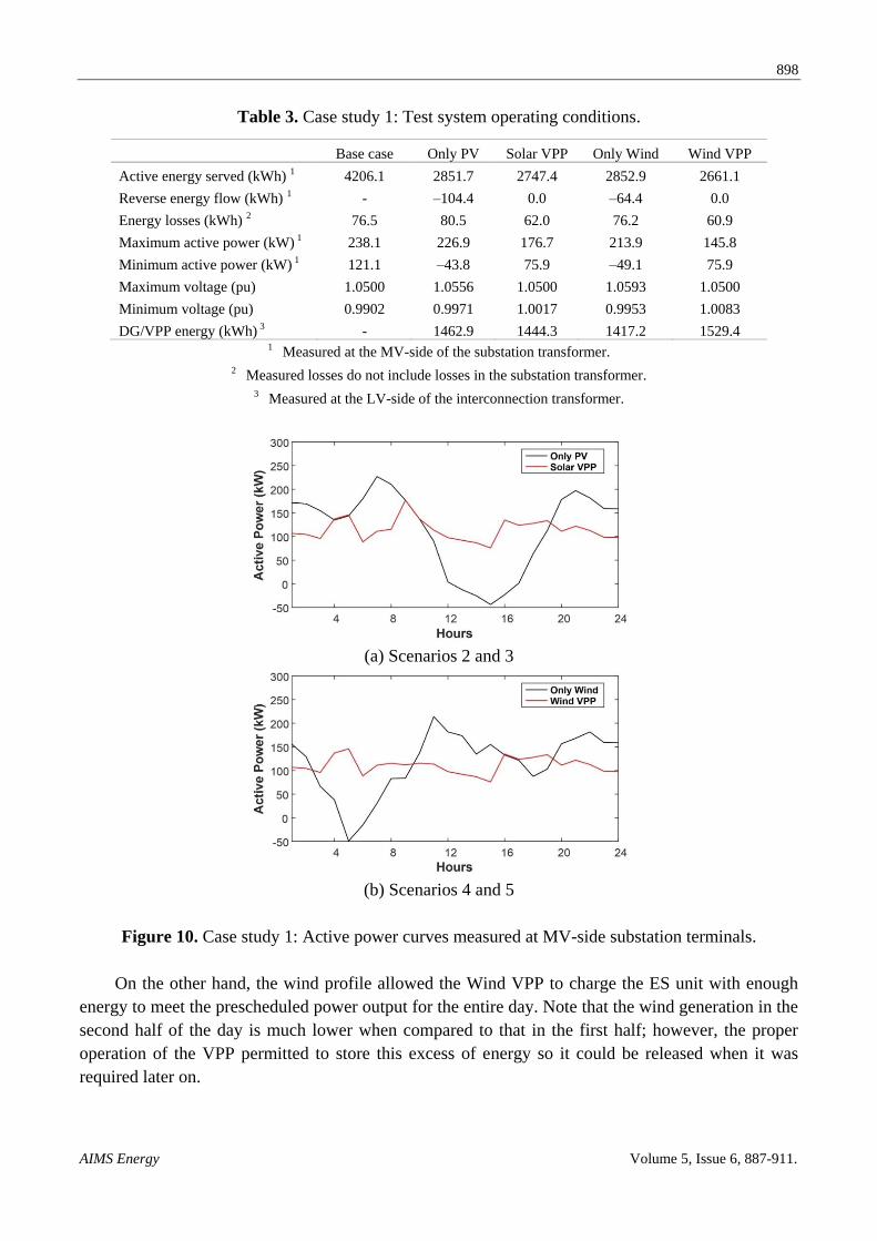
Table 3. Case study 1: Test system operating conditions.
Base case Only PV Solar VPP Only Wind Wind VPP
Active energy served (kWh) 1 4206.1 2851.7 2747.4 2852.9 2661.1
Reverse energy flow (kWh) 1 - –104.4 0.0 –64.4 0.0
Energy losses (kWh) 2 76.5 80.5 62.0 76.2 60.9
Maximum active power (kW) 1 238.1 226.9 176.7 213.9 145.8
Minimum active power (kW) 1 121.1 –43.8 75.9 –49.1 75.9
Maximum voltage (pu) 1.0500 1.0556 1.0500 1.0593 1.0500
Minimum voltage (pu) 0.9902 0.9971 1.0017 0.9953 1.0083
DG/VPP energy (kWh) 3 - 1462.9 1444.3 1417.2 1529.4 1 Measured at the MV-side of the substation transformer.
2 Measured losses do not include losses in the substation transformer.
3 Measured at the LV-side of the interconnection transformer.
(a) Scenarios 2 and 3
(b) Scenarios 4 and 5
Figure 10. Case study 1: Active power curves measured at MV-side substation terminals.
On the other hand, the wind profile allowed the Wind VPP to charge the ES unit with enough
energy to meet the prescheduled power output for the entire day. Note that the wind generation in the
second half of the day is much lower when compared to that in the first half; however, the proper
operation of the VPP permitted to store this excess of energy so it could be released when it was
required later on.
899
AIMS Energy Volume 5, Issue 6, 887-911.
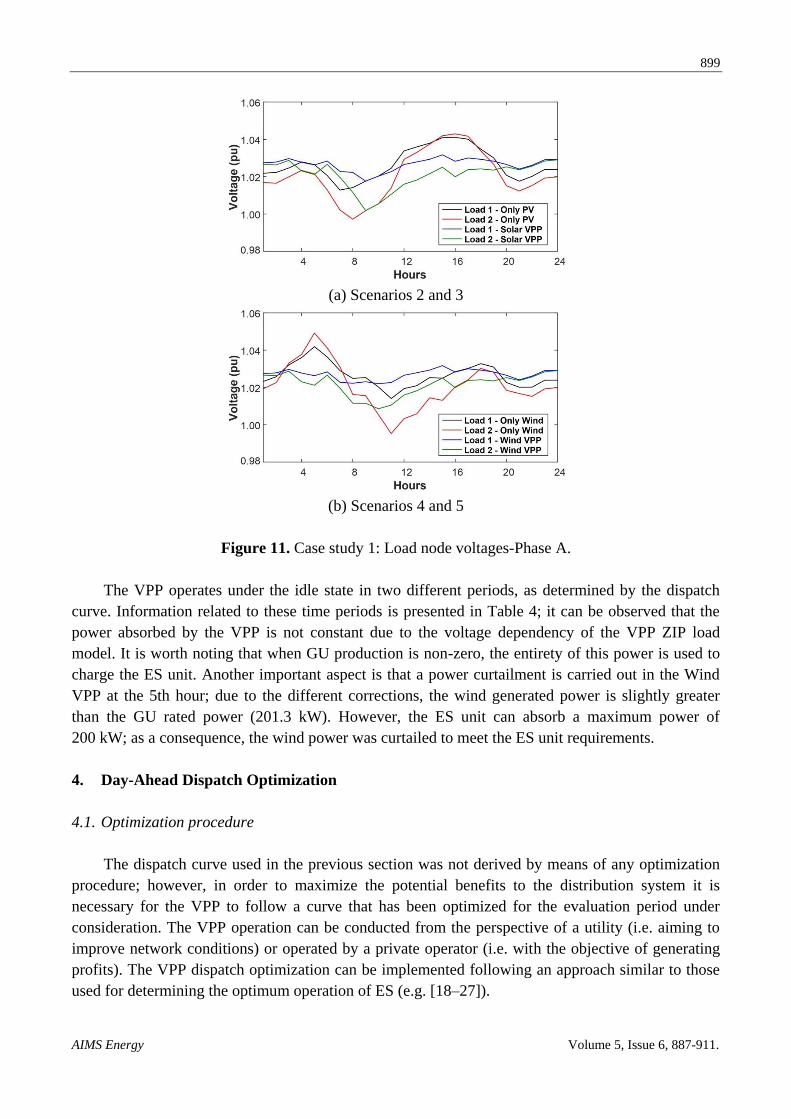
(a) Scenarios 2 and 3
(b) Scenarios 4 and 5
Figure 11. Case study 1: Load node voltages-Phase A.
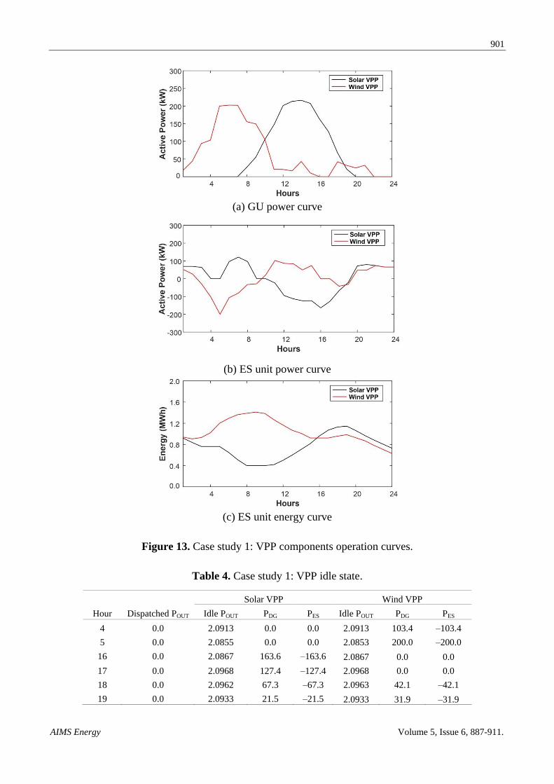
The VPP operates under the idle state in two different periods, as determined by the dispatch
curve. Information related to these time periods is presented in Table 4; it can be observed that the
power absorbed by the VPP is not constant due to the voltage dependency of the VPP ZIP load
model. It is worth noting that when GU production is non-zero, the entirety of this power is used to
charge the ES unit. Another important aspect is that a power curtailment is carried out in the Wind
VPP at the 5th hour; due to the different corrections, the wind generated power is slightly greater
than the GU rated power (201.3 kW). However, the ES unit can absorb a maximum power of
200 kW; as a consequence, the wind power was curtailed to meet the ES unit requirements.
4. Day-Ahead Dispatch Optimization
4.1. Optimization procedure
The dispatch curve used in the previous section was not derived by means of any optimization
procedure; however, in order to maximize the potential benefits to the distribution system it is
necessary for the VPP to follow a curve that has been optimized for the evaluation period under
consideration. The VPP operation can be conducted from the perspective of a utility (i.e. aiming to
improve network conditions) or operated by a private operator (i.e. with the objective of generating
profits). The VPP dispatch optimization can be implemented following an approach similar to those
used for determining the optimum operation of ES (e.g. [18–27]).
900
AIMS Energy Volume 5, Issue 6, 887-911.
(a) Scenarios 2 and 3
(b) Scenarios 4 and 5
Figure 12. Case study 1: Active power output.
Day-ahead dispatch is based on the system’s forecast for the following day; the VPP operation
must be optimized according to these forecasted load and renewable resource curves. This section
presents a procedure for determining the optimal hourly day-ahead dispatch of multiple VPPs from
the utility’s perspective.
In this section the VPP optimal dispatch is determined by means of a general parallel genetic
algorithm (GPGA). The implemented GPGA is a global single-population GA [28], where only one
population is created and the evaluation of each member of a given generation is independent from
the rest of the members; therefore, the evaluation of a generation can be seen as an embarrassingly
parallel problem [29]. This approach yields a reduction of the total execution times by distributing
the evaluation of individuals in a generation among available cores in a multi-core installation.
The GPGA will seek to determine the optimal values for every point of the VPP operation curve
that minimize the following operation variables:
Distribution energy losses, without including losses in substation transformer (EL).
Energy supplied from the MV-side of the substation transformer (E).
Peak power supplied by the substation transformer from the MV-side terminals (PMAX).
For a day-ahead dispatch with a 1-hour time step, the VPP operation curve will consist of 24
values, which can be either positive or negative (according to the power injection or absorption).
Note that the procedure can cope with multiple dispatch curves; that is, different VPPs can follow
different operation curves. The parameters used in the optimization procedure are shown in Table 5.
901
AIMS Energy Volume 5, Issue 6, 887-911.
(a) GU power curve
(b) ES unit power curve
(c) ES unit energy curve
Figure 13. Case study 1: VPP components operation curves.
Table 4. Case study 1: VPP idle state.
Solar VPP Wind VPP
Hour Dispatched POUT Idle POUT PDG PES Idle POUT PDG PES
4 0.0 2.0913 0.0 0.0 2.0913 103.4 –103.4
5 0.0 2.0855 0.0 0.0 2.0853 200.0 –200.0
16 0.0 2.0867 163.6 –163.6 2.0867 0.0 0.0
17 0.0 2.0968 127.4 –127.4 2.0968 0.0 0.0
18 0.0 2.0962 67.3 –67.3 2.0963 42.1 –42.1
19 0.0 2.0933 21.5 –21.5 2.0933 31.9 –31.9
902
AIMS Energy Volume 5, Issue 6, 887-911.
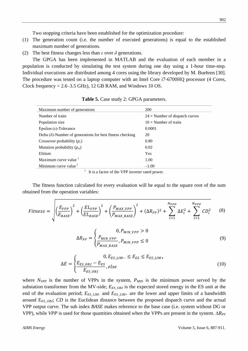
Two stopping criteria have been established for the optimization procedure:
(1) The generation count (i.e. the number of executed generations) is equal to the established
maximum number of generations.
(2) The best fitness changes less than ε over δ generations.
The GPGA has been implemented in MATLAB and the evaluation of each member in a
population is conducted by simulating the test system during one day using a 1-hour time-step.
Individual executions are distributed among 4 cores using the library developed by M. Buehren [30].
The procedure was tested on a laptop computer with an Intel Core i7-6700HQ processor (4 Cores,
Clock frequency = 2.6–3.5 GHz), 12 GB RAM, and Windows 10 OS.
Table 5. Case study 2: GPGA parameters.
Maximum number of generations 200
Number of traits 24 × Number of dispatch curves
Population size 10 × Number of traits
Epsilon (ε)-Tolerance 0.0001
Delta (δ)-Number of generations for best fitness checking 20
Crossover probability (pc) 0.80
Mutation probability (pm) 0.02
Elitism Yes
Maximum curve value 1 1.00
Minimum curve value 1 –1.00 1 It is a factor of the VPP inverter rated power.
The fitness function calculated for every evaluation will be equal to the square root of the sum
obtained from the operation variables:
(8)
(9)
(10)
where NVPP is the number of VPPs in the system, PMIN is the minimum power served by the
substation transformer from the MV-side; EES_OBJ is the expected stored energy in the ES unit at the
end of the evaluation period; EES_LIM– and EES_LIM+ are the lower and upper limits of a bandwidth
around EES_OBJ; CD is the Euclidean distance between the proposed dispatch curve and the actual
VPP output curve. The sub index BASE makes reference to the base case (i.e. system without DG or
VPP), while VPP is used for those quantities obtained when the VPPs are present in the system. ∆RPF
903
AIMS Energy Volume 5, Issue 6, 887-911.
has been introduced in the fitness function as penalty for those cases in which reverse power flow
occurs, while ∆E is a penalty for those cases when the ES unit stored energy falls outside of the
bandwidth defined by EES_LIM– and EES_LIM+. Forcing the ES unit to maintain a minimum value of
stored energy at the end of the evaluation period will ensure that the VPP will have enough energy
for meeting the following day’s dispatch (i.e. the day after the day-ahead).
The procedure seeks to minimize the value of the fitness function presented in Equation (8). For
every evaluation, the procedure checks that all voltages are within accepted limits (between 0.95 and
1.05 pu), no network element experiences overload, and the iterative algorithm converges for all
solution steps. If one or more of these conditions are not fulfilled, the procedure will assign a large
value to the fitness function, which will make difficult its participation in the subsequent generations
of the GPGA.
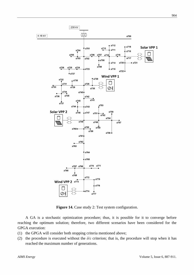
4.2. Test system configuration
The new test system prepared for this case study is a three-phase 60-Hz overhead system with a
simplified representation of the HV transmission system (see Figure 14). VPPs use the same
configuration as in the previous test system, see Figures 3 through 7. By default, all distribution loads
are connected to the system through MV/LV transformers.
Some important information related to the new test system follows:
HV rated voltage: 230 kV.
HV actual voltage: 1.03 pu.
MV rated voltage: 4.16 kV.
LV rated voltage: 0.4 kV.
Substation transformer rated power: 2500 kVA.
Total rated active load: 1700 kW.
As in Test System 1, loads have been modelled as voltage-independent and curve shapes have
been derived with the procedure presented in [14].
Solar VPP 1 and Wind VPP 1 use the same parameters as those in case study 1; furthermore, the
expected stored energy, and lower and upper bandwidth limits have been set to 1500, 800, and
1200 kWh, respectively. The characteristics of Solar VPP 2 and Wind VPP 2 are presented in
Table 6 (all VPPs operate under the Dispatch operation mode). Note that the rated values and
locations of all VPPs have been arbitrarily chosen. It is assumed that the solar irradiance and
reference wind speed are the same for the entire system; due to height corrections the actual wind
speed curve will be different for both Wind VPPs.
4.3. Simulation results
The GPGA was executed to obtain the optimal day-ahead dispatch of active power for the VPPs
in the system. Due to the different nature of wind and solar resources, the procedure will derive two
dispatch curves: the first one will be assigned to the Solar VPPs, while the Wind VPPs will operate
according to the second dispatch curve. As in the previous study, the selected 24 hours belong to a
specific day of the year, and the load curves for the previous and following day present different
values and characteristics.
904
AIMS Energy Volume 5, Issue 6, 887-911.
Figure 14. Case study 2: Test system configuration.
A GA is a stochastic optimization procedure; thus, it is possible for it to converge before
reaching the optimum solution; therefore, two different scenarios have been considered for the
GPGA execution:
(1) the GPGA will consider both stopping criteria mentioned above;
(2) the procedure is executed without the δ/ε criterion; that is, the procedure will stop when it has
reached the maximum number of generations.
905
AIMS Energy Volume 5, Issue 6, 887-911.
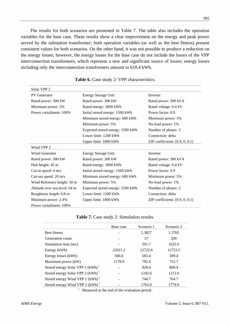
The results for both scenarios are presented in Table 7. The table also includes the operation
variables for the base case. These results show a clear improvement on the energy and peak power
served by the substation transformer; both operation variables (as well as the best fitness) present
consistent values for both scenarios. On the other hand, it was not possible to produce a reduction on
the energy losses; however, the energy losses for the base case do not include the losses of the VPP
interconnection transformers, which represent a new and significant source of losses; energy losses
including only the interconnection transformers amount to 618.4 kWh.
Table 6. Case study 2: VPP characteristics.
Solar VPP 2
PV Generator Energy Storage Unit Inverter
Rated power: 300 kW Rated power: 300 kW Rated power: 300 kVA
Minimum power: 5% Rated energy: 3000 kWh Rated voltage: 0.4 kV
Power curtailment: 100% Initial stored energy: 1500 kWh Power factor: 0.9
Minimum stored energy: 600 kWh Minimum power: 5%
Minimum power: 5% No-load power: 1%
Expected stored energy: 1500 kWh Number of phases: 3
Lower limit: 1200 kWh Connection: delta
Upper limit: 1800 kWh ZIP coefficients: [0.9, 0, 0.1]
Wind VPP 2
Wind Generator Energy Storage Unit Inverter
Rated power: 300 kW Rated power: 300 kW Rated power: 300 kVA
Hub height: 45 m Rated energy: 3000 kWh Rated voltage: 0.4 kV
Cut-in speed: 4 m/s Initial stored energy: 1500 kWh Power factor: 0.9
Cut-out speed: 20 m/s Minimum stored energy: 600 kWh Minimum power: 5%
Wind Reference height: 50 m Minimum power: 5% No-load power: 1%
Altitude over sea-level: 64 m Expected stored energy: 1500 kWh Number of phases: 3
Roughness length: 0.8 m Lower limit: 1200 kWh Connection: delta
Minimum power: 2.4% Upper limit: 1800 kWh ZIP coefficients: [0.9, 0, 0.1]
Power curtailment: 100%
Table 7. Case study 2: Simulation results.
Base case Scenario 1 Scenario 2
Best fitness - 1.3827 1.3765
Generation count - 57 200
Simulation time (sec) - 501.7 1625.0
Energy (kWh) 22021.2 12722.6 12753.5
Energy losses (kWh) 566.6 583.4 589.4
Maximum power (kW) 1178.9 792.4 752.7
Stored energy Solar VPP 1 (kWh) 1 - 828.4 808.4
Stored energy Solar VPP 2 (kWh) 1 - 1242.6 1212.6
Stored energy Wind VPP 1 (kWh) 1 - 744.7 764.7
Stored energy Wind VPP 2 (kWh) 1 - 1763.9 1779.9 1 Measured at the end of the evaluation period.
906
AIMS Energy Volume 5, Issue 6, 887-911.
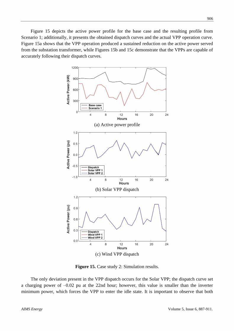
Figure 15 depicts the active power profile for the base case and the resulting profile from
Scenario 1; additionally, it presents the obtained dispatch curves and the actual VPP operation curve.
Figure 15a shows that the VPP operation produced a sustained reduction on the active power served
from the substation transformer, while Figures 15b and 15c demonstrate that the VPPs are capable of
accurately following their dispatch curves.
(a) Active power profile
(b) Solar VPP dispatch
(c) Wind VPP dispatch
Figure 15. Case study 2: Simulation results.
The only deviation present in the VPP dispatch occurs for the Solar VPP; the dispatch curve set
a charging power of –0.02 pu at the 22nd hour; however, this value is smaller than the inverter
minimum power, which forces the VPP to enter the idle state. It is important to observe that both
907
AIMS Energy Volume 5, Issue 6, 887-911.
dispatch curves present different behaviors throughout the evaluation period, which is likely to be
caused by the different nature of both resources.
Due to difference in hub height, the Wind VPP 2 will produce more power and energy (in pu)
than the Wind VPP 1; as a result, the stored energy in the ES unit at the end of the evaluation
period (with respect to the rated energy) will also be greater, see Table 7. In general, the stored
energy in the Wind VPP 2 at the end of the evaluation period is always close to the bandwidth’s
upper limit, which means that the VPP could inject more energy into the system and still remain
within the desired bandwidth; however, the Wind VPP 2 cannot use this extra energy if it is forced to
follow the same dispatch curve as the Wind VPP 1. In order to explore the possibility of utilizing the
extra energy stored in the Wind VPP 2, the GPGA has been executed considering one dispatch curve
for each Wind VPP. Additionally, the GPGA was also executed considering one dispatch curve per
VPP (i.e. 4 dispatch curves). Simulation results for these new conditions are presented in Table 8.
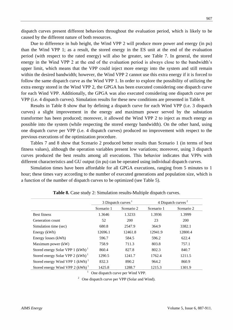
Results in Table 8 show that by defining a dispatch curve for each Wind VPP (i.e. 3 dispatch
curves) a slight improvement in the energy and maximum power served by the substation
transformer has been produced; moreover, it allowed the Wind VPP 2 to inject as much energy as
possible into the system (while respecting the stored energy bandwidth). On the other hand, using
one dispatch curve per VPP (i.e. 4 dispatch curves) produced no improvement with respect to the
previous executions of the optimization procedure.
Tables 7 and 8 show that Scenario 2 produced better results than Scenario 1 (in terms of best
fitness values), although the operation variables present low variations; moreover, using 3 dispatch
curves produced the best results among all executions. This behavior indicates that VPPs with
different characteristics and GU output (in pu) can be operated using individual dispatch curves.
Simulation times have been affordable for all GPGA executions, ranging from 5 minutes to 1
hour; these times vary according to the number of executed generations and population size, which is
a function of the number of dispatch curves to be optimized (see Table 5).
Table 8. Case study 2: Simulation results-Multiple dispatch curves.
3 Dispatch curves 1 4 Dispatch curves 2
Scenario 1 Scenario 2 Scenario 1 Scenario 2
Best fitness 1.3646 1.3233 1.3936 1.3999
Generation count 52 200 23 200
Simulation time (sec) 680.8 2547.9 364.9 3382.1
Energy (kWh) 12696.1 12461.8 12941.9 12800.4
Energy losses (kWh) 596.7 584.5 596.2 622.4
Maximum power (kW) 758.9 711.3 803.8 757.1
Stored energy Solar VPP 1 (kWh) 1 860.4 827.8 802.3 840.7
Stored energy Solar VPP 2 (kWh) 1 1290.5 1241.7 1762.4 1211.5
Stored energy Wind VPP 1 (kWh) 1 832.3 890.2 964.2 860.9
Stored energy Wind VPP 2 (kWh) 1 1425.8 1288.7 1215.3 1301.9 1 One dispatch curve per Wind VPP.
2 One dispatch curve per VPP (Solar and Wind).
908
AIMS Energy Volume 5, Issue 6, 887-911.
5. Conclusions
This paper has presented a virtual power plant model for power flow calculations. The model
has been compiled as a custom-made capability within the OpenDSS COM DLL and can be used in
time-driven simulations controlled from other software platforms, e.g. MATLAB. The model has the
same capabilities as other OpenDSS objects and it can be defined, modified, and accessed using the
same methods.
Two different operation modes have been implemented inside the model: Follow and Dispatch.
Under the Follow mode the model behaves according to the curves assigned to the GU and ES unit,
whereas in Dispatch mode the VPP acts as a dispatchable unit.
The list of features implemented in the model includes: (i) active and reactive power
dispatch, (ii) power curtailment, (iii) inverter idle power modeled as a ZIP load, (iv) minimum power
limit for GU and ES unit, (v) automatic calculation of ES unit maximum charge/discharge power,
and (vi) inverter power limits.
The first case study has shown how the VPP can make better use of the renewable resources,
since it is capable of storing the generation surplus and injecting it into the network during low
generation periods; the presence of ES is essential for meeting the power dispatch curve.
Contrary to DG based only on intermittent resources, the VPP output can be adjusted to meet
the system requirements and thus avoid undesired operating conditions, such as system voltages
above accepted limits. This is a vital feature for achieving larger penetration factors of renewable
generation without compromising normal system operation.
The VPP can help to further improve system operating conditions by injecting or absorbing
reactive power; the absorption of reactive power is expected to play a key role if the objective is to
export energy to the transmission system [31].
The paper has also presented a procedure for determining the optimal day-ahead dispatch for the
VPP based on a GPGA. The procedure seeks to explore the potential improvement on the overall
operating conditions when the VPP is operated from the perspective of a utility. The presented
methodology relies on a power flow simulator (i.e. OpenDSS) for calculating the system operating
conditions; namely, no simplifications are introduced into the solution of the electrical system.
Furthermore, the evaluated system can be of any size and include detailed models and control
algorithms for system components (e.g. the presented VPP model). An accurate calculation of system
conditions is essential for the optimization methodology since a poor estimation would cause the
procedure to produce erroneous results.
A genetic algorithm requires a large number of executions in order to produce accurate results;
although each individual execution does not require large simulation times, the repeated evaluation
of the system could result in prohibitive executions times if they were to be performed in a sequential
manner (i.e. using single core computing). This work makes use of parallel computing in
combination with the GA (i.e. a GPGA) in order to distribute the individual executions among the
available cores to produce a reduction in the total execution times.
The results presented in the second case study show that the proposed optimization procedure is
capable of producing significant improvements on the system conditions and that the parallel
approach used in this work produces affordable simulation times. These simulation times could be
further reduced through the use of a larger multi-core installation.
909
AIMS Energy Volume 5, Issue 6, 887-911.
Similar results to those presented in this paper could be achieved by defining appropriate
operation curves of an OpenDSS Storage object that works in conjunction with the PV System or
Generator objects; however, the coordination between both objects should be handled by an external
tool (e.g. MATLAB), which would represent a significant loss in performance. The main advantage
of the present model is that all operations and control decisions are compiled within the COM DLL,
which makes them seamless to the user and helps to maintain the high computing performance of
OpenDSS.
In its present form the developed VPP model is adequate for exploring the effect that the
aggregation of renewable generation and energy storage can have on the system. Future work could
be aimed at expanding the VPP model to incorporate losses in the DC network and implement an
algorithm to automatically control the inverter’s reactive power based on the system’s conditions.
Furthermore, an optimization procedure must be implemented in order to determine the optimal VPP
operation curve for an extended evaluation period (i.e. one year or more).
Conflict of Interest
The author declares no conflicts of interest in this paper.
References
1. Willis HL, Scott WG (2000) Distributed power generation. Planning and evaluation. CRC Press.
2. Ackermann T, Andersson G, Söder L (2001) Distributed generation: a definition. Electr Pow Syst
Res 57: 195–204.
3. Mahmoud PHA, Huy PD, Ramachandaramurthy VK (2017) A review of the optimal allocation of
distributed generation: objectives, constraints, methods, and algorithms. Renew Sust Energ Rev
75: 293–312.
4. Sandia National Laboratories and NRECA (2015) DOE/EPRI Electricity Storage Handbook.
5. Li X, Hui D, Lai X (2013) Battery energy storage station (BESS)-based smoothing control of
photovoltaic (PV) and wind power generation fluctuations. IEEE T Sustain Energ 4: 464–473.
6. Grillo S, Marinelli M, Massucco S, et al. (2012) Optimal management strategy of a battery-based
storage system to improve renewable energy integration in distribution networks. IEEE T Smart
Grid 3: 950–958.
7. Katsanevakis M, Stewart RA, Lu J (2017) Aggregated applications and benefits of energy storage
systems with application-specific control methods: a review. Renew Sust Energ Rev 75: 719–741.
8. Etherden N, Vyatkin V, Bollen MHJ (2016) Virtual power plant for grid services using IEC
61850. IEEE T Ind Inform 12: 437–447.
9. International Electrotechnical Commission (2011) Electrical Energy Storage. Available from:
https://www.mendeley.com/research-papers/electrical-energy-storage-white-paper-3/.
10. Dugan RC (2016) Reference Guide. The Open Distribution System Simulator (OpenDSS). EPRI.
11. Pudjianto D, Ramsay C, Strbac G (2007) Virtual power plant and system integration of
distributed energy resources. Iet Renew Power Gen 1: 10–16.
12. Ghavidel S, Li L, Aghaei J, et al. (2016) A review on the virtual power plant: Components and
operation systems. IEEE International Conference on Power System Technology. IEEE, 1–6.
910
AIMS Energy Volume 5, Issue 6, 887-911.
13. Kolenc M, Nemček P, Gutschi C, et al. (2017) Performance evaluation of a virtual power plant
communication system providing ancillary services. Electr Pow Syst Res 149: 46–54.
14. Martínez-Velasco JA, Guerra G (2015) Analysis of large distribution networks with distributed
energy resources. Ingeniare 23: 594–608.
15. Dugan RC, Taylor JA, Montenegro D (2017) Energy storage modeling for distribution planning.
IEEE T Ind Appl 53: 954–962.
16. Chassin DP (2013) Electrical load modeling and simulation. In: Khaitan SK, Gupta A, editors,
High Performance Computing in Power and Energy Systems, Berlin: Springer.
17. Guerra G, Martinez-Velasco JA (2017) A solid state transformer model for power flow
calculations. Int J Elec Power 89: 40–51.
18. Farzin H, Fotuhi-Firuzabad M, Moeini-Aghtaie M (2017) A stochastic multi-objective
framework for optimal scheduling of energy storage systems in microgrids. IEEE T Smart Grid 8:
117–127.
19. Levron Y, Shmilovitz D (2012) Power systems’ optimal peak-shaving applying secondary
storage. Electr Pow Syst Res 89: 80–84.
20. Jayasekara N, Wolfs P, Masoum MAS (2014) An optimal management strategy for distributed
storages in distribution networks with high penetrations of PV. Electr Pow Syst Res 116: 147–
157.
21. Meirinhos JL, Rua DE, Carvalho LM, et al. (2017) Multi-temporal optimal power flow for
voltage control in MV networks using distributed energy resources. Electr Pow Syst Res 146: 25–
32.
22. Hejazi H, Mohsenian-Rad H (2016) Energy storage planning in active distribution grids: a
chance-constrained optimization with non-parametric probability functions. IEEE T Smart Grid:
1–13.
23. Silvestre MLD, Graditi G, Ippolito MG, et al. (2011) Robust multi-objective optimal dispatch of
distributed energy resources in micro-grids. Power Tech, 2011 IEEE Trondheim. IEEE, 1–5.
24. Agamah SU, Ekonomou L (2016) Peak demand shaving and load-levelling using a combination
of bin packing and subset sum algorithms for electrical energy storage system scheduling. Iet Sci
Meas Technol 10: 477–484.
25. Qin J, Sevlian R, Varodayan D, et al. (2012) Optimal electric energy storage operation. 2012
IEEE Power and Energy Society General Meeting, 1–6.
26. Pandzic H, Kuzle I (2015) Energy storage operation in the day-ahead electricity market.
European Energy Market. IEEE, 1–6.
27. Lazaroiu GC, Dumbrava V, Balaban G, et al. (2016) Stochastic optimization of microgrids with
renewable and storage energy systems. IEEE, International Conference on Environment and
Electrical Engineering.
28. Yeh EC, Venkata SS, Sumic Z (1996) Improved distribution system planning using
computational evolution. IEEE T Power Syst 11: 668–674.
29. Konfrst Z (2004) Parallel genetic algorithms: advances, computing trends, applications and
perspectives. Parallel and Distributed Processing Symposium. Proceedings. International. IEEE,
162.
30. Buehren M. MATLAB Library for Parallel Processing on Multiple Cores. Available from
http://www.mathworks.com.
911
AIMS Energy Volume 5, Issue 6, 887-911.
31. Kieny C, Berseneff B, Hadjsaid N, et al. (2009) On the concept and the interest of Virtual Power
plant: Some results from the European project FENIX. Power & Energy Society General Meeting,
IEEE, 1–6.
© 2017 Juan A. Martinez Velasco, et al., licensee AIMS Press. This is an
open access article distributed under the terms of the Creative Commons
Attribution License (http://creativecommons.org/licenses/by/4.0)