Embed Size (px)
Citation preview

1
Journal of Applied Statistics, Vol. 29, No.8, pp. 1165-1179, 2002
A Versatile Bivariate Distribution on a Bounded Domain:
Another Look at the Product Moment Correlation
SAMUEL KOTZ & J. RENÉ VAN DORP, Department of Engineering Management and
Systems Engineering, The George Washington University, Washington, D.C.
Abstract - The Fairlie-Gumbel-Morgenstern (FGM) family has been investigated in detail for
various continuous marginals such as Cauchy, normal, exponential, gamma, Weibull, lognormal
and others. It has been a popular model for the bivariate distribution with mild dependence.
However, bivariate FGM’s with continuous marginals on a bounded support discussed in the
literature are only those with uniform or power marginals. In this note we study the bivariate
FGM family with marginals given by the recently proposed two-sided power (TSP) distribution.
Since this family of bounded continuous distributions is very flexible, the properties of the FGM
family with TSP marginals could serve a reliable indication of the structure of the FGM
distribution with arbitrary marginals defined on a compact set. A remarkable stability of the
correlation between the marginals has been observed.
1. INTRODUCTION
The arsenal for constructing continuous bivariate distribution with specified marginals on a
bounded set is rather limited. Most continuous bivariate distributions with specified marginals
are constructed on either the whole or on a positive orthant. This is due mainly to the fact that�#
the vast majority of univariate continuous distributions are defined on an infinite interval (with
Correspondence: J.R. van Dorp, Department of Engineering Management and Systems Engineering, School of
Engineering and Applied Science, 1776 G Street, N.W., Suite 110, The George Washington University, Washington,
D.C. 20052, US. E-mail: [email protected]

2
Journal of Applied Statistics, Vol. 29, No.8, pp. 1165-1179, 2002
the notable exceptions of the beta distribution - and its particular cases uniform and power
distributions - and the triangular distributions.) Indeed, the by far most widely used continuous
distribution on a bounded interval is the uniform followed by the beta distribution, the power
distribution and only recently some attention has began to be paid to the triangular distribution
(see, e.g., . The fact that bivariate distributionsJohnson (1997) and Johnson and Kotz (1999))
with specified continuous marginals have not been investigated for the case of beta marginals
may partially be explained by the fact that specification of marginals requires the use of the
cumulative distribution function (cdf) in a closed form, not available for this distribution.
Actually, to the best of our knowledge, even bivariate distributions with specified triangular
marginals have not been studied. While the Dirichlet and Ordered Dirichlet distribution are
multivariate distributions with beta marginals (on a bounded support), they do not allow for
arbitrary specification of beta marginals (see e.g. Kotz et al. (2000) and Van Dorp et al. (1996)).
It would seem that construction of bivariate distributions with marginals witharbitrary specified
bounded support may still be considered an unchartered area.
Fortunately there exist several mechanisms for constructing bivariate distributions. A new
method of generating bivariate distribution based on the modification of a bivariate uniform
distribution and a subsequent "cloning" has been proposed by Johnson and Kotz (2001). Earlier
mechanisms for constructing bivariate distributions with arbitrary specified marginals center
around the use of copulas (see, e.g., Genest and Mackay (1986)). The easiest and most natural
approach embodied in the general class of bivariate distributions is perhaps the one originally
proposed by Morgenstern (1956), Gumbel (1960) and Farlie (1960) known in the literature as the
FGM family. This family has only one governing parameter which determines the degree of
dependence (in addition to the parameters of the marginal distributions). A vast literature on this
topic exists (see, e.g., by now the recent book by Drouet and Kotz (2001)).
The starting point for the constructing of a FGM family is the case of uniform marginals.
Here the bivariate cdf is given by

3
Journal of Applied Statistics, Vol. 29, No.8, pp. 1165-1179, 2002
� �� � � � � � � �� �� � ��� � ��� � � �� � � � � �� � � �� �� ���Y ÄY " # " # " # 3" #� �
and the pdf is simply
� �� � � � � �� �� �� ��� �� ��� � � �� � � � � �� � � �� �� ���Y ÄY " # " # 3" #� �
In general a FGM bivariate distribution with marginal cdf’s and pdf’s� �� �� � �� �\ " \ #" #
� �� �� � �� ��\ " \ #" #is represented as
� �� � � � � �� �� �� �� ���\ Ä\ " #" #� �� �� �� � � �� �� � �� ��\ " \ # \ " \ #" # " #
�
or in terms of pdf’s (if they exist) as
� �� � � � � � �� �� �� �� �� �� ���\ Ä\ " #" # \ " # \ " \ #\" " ##�� �� �� � �� �� �� ���
where as above � � �� � � � � �� � � �� ��� 3 The basic theory of FGM distributions and its
correlation structure has been investigated for various continuous marginals with unbounded
support such as Cauchy, Normal, exponential, gamma, Weibull, lognormal and many others in
Johnson and Kotz (1975), (1977), Schucany et al. (1978), Cook and Johnson (1986), D’ Este
(1981), Lingappaiah (1984), Barnett (1965) and Drouet and Kotz (2001), among other sources.
As to FGM distributions with bounded support, besides those with uniform marginals, only the
case of power marginals with the density seem to receive� ��� � �� � � � � � �� � � �\8�"
any attention. (See, e.g., Schucany et al. (1978)).
The product moment correlation coefficient for the FGM distributions with continuousall
marginals is less than / with the maximum being attained for the uniform marginals. The� �
model is thus applicable to the cases of a "mild" correlation which occurs in engineering and
medical applications (see, e.g., Blischke and Prabhaker Murthy (2000) and Chalabian and
Dunnington (1998)). The maximum correlation coefficient for normal marginals is , for�� ����
exponential marginals, for the Laplace and gamma marginals (with the shape parameter�����
equal to ) and is (ranging from to for power marginals.� ��� ������ �� � ����#

4
Journal of Applied Statistics, Vol. 29, No.8, pp. 1165-1179, 2002
We shall study the correlation structure of a bivariate FGM family with marginals given by
the two parameter, two-sided power (TSP) distribution introduced by van Dorp and Kotz
(2001a,b). The distribution in its canonical form is given by the cdf
� ��� � ���� � � �
� �� � � � � �\ 8
B8
"�B"�
������ �
� �� �
� �
)
)
and the density
� ��� � ���� � � �
� � � ��\
B8�"
"�B"�
8�"
������ �� �
)
)
�
�
where 1, The mean and the variance of the random variable are� � � � � �� ��
���� � �� � ����� ��
� ��
� 1
and
!"��� � �� � ���� ��� �� �� �
�� ���� ���
� �#
,
respectively. We shall denote this family using the abbreviation . This family of#$%� � ���
bounded continuous distributions is so flexible and versatile that it is very likely that the FGM
family with the TSP marginals may serve as a reliable indicator of the structure of FGM
distributions with arbitrary "non-pathological" marginals defined on a compact set. The
flexibility of the TSP distribution is similar to that of the beta distribution and both families
include U-Shaped , , J-Shaped ) and unimodal ( , or�� � & ��� ��� � & '�� �( � � � & ��� ��� � �
� & '�� �(� forms and posses the same limiting distributions (See, Van Dorp and Kotz (2001a)).
The uniform distribution , power distribution ( and triangular distribution �� � �� � �� �� � ���
all belong to the family. Similarly to the power distribution the TSP family is not a#$%� � ���
location-scale family thus yielding a product moment correlation coefficient function of the
marginal parameters (unlike the uniform, normal, exponential and lognormal distributions). In

5
Journal of Applied Statistics, Vol. 29, No.8, pp. 1165-1179, 2002
Section 3, the correlation coefficient for the FGM family with TSP marginals is derived as a
function of the parameters. We investigate the extremes of this correlation coefficient and its
behavior in Section 4. Finally, we shall provide some concluding remarks in Section 5.
2. THE DENSITY
Let be the joint density function given by where ( ) are � �� � � � ��� � � � �� � #$% � � � �\ Ä\ " # 3 3 3" #�
random variables with cdf and pdf given by and respectively. Figures 1 provide some��� ���
illustrative examples of the joint density with identical marginals for a variety of� �� � � �\ Ä\ " #" #
#$%� � � � � ��� �3 3 scenarios with Figure 1A displays the bivariate FGM with uniform
marginals , Figure B depicts the bivariate FGM with power marginals ( ,�� � �� � � �� � � ��3 3 3�
Figure C displays the bivariate FGM with symmetric triangular marginals ( and� � � � � ���3 3"#
Figure 1D presents the bivariate FGM with genuine symmetric TSP marginals (�3 3"#� � � � ���
Figures provide some additional examples of the joint density with and� � �� � � � � �\ Ä\ " #" #�
non-identical , marginals Figure 2A displays the FGM density with TSP#$%� � � � � � �� �� ��3 3
marginals with , Figure 2B depicts the FGM density with TSP marginals� � � � �� � � ��" # #�
with , Figure 2C presents the FGM density with TSP marginals with� � � � � � � �)" # #"#�
� �" " # #� �� � � � � �� � � ��, Figure 2D displays the FGM density with symmetric but unequal
TSP marginals where , .� �" " # #" " "# # #� � � � � � � � �
It is evident from Figures 1 and 2 that the form of the joint density functions of an FGM
distribution with TSP marginals can take great variety of forms. It is therefore of interest to
investigate the corresponding correlation structure.

6
Journal of Applied Statistics, Vol. 29, No.8, pp. 1165-1179, 2002
0.00
0.50
1.00
1.50
2.00
2.50
0.00 0.50 1.00
X1
PD
F
(0,0) (1,1)
A
(0,0) (1,1)
C
(0,0) (1,1)
D
0.00
0.20
0.40
0.60
0.80
1.00
1.20
0.00 0.50 1.00
X1
PD
F
0.00
0.20
0.40
0.60
0.80
1.00
1.20
0.00 0.50 1.00
X2
PD
F
0.00
0.50
1.00
1.50
2.00
2.50
0.00 0.50 1.00
X1
PD
F
0.00
0.50
1.00
1.50
2.00
2.50
0.00 0.50 1.00
X2
PD
F
0.00
0.50
1.00
1.50
2.00
2.50
3.00
3.50
0.00 0.50 1.00
X1
PD
F
0.00
0.50
1.00
1.50
2.00
2.50
3.00
3.50
0.00 0.50 1.00
X2
PD
F
x1x2
x1x2
x1x2
JOIN
T P
DF
JOIN
T P
DF
JOIN
T P
DF
(0,0) (1,1)x1
x2
JOIN
T P
DF
MA
RG
INA
L P
DF
MA
RG
INA
L P
DF
MA
RG
INA
L P
DF
MA
RG
INA
L P
DF
MA
RG
INA
L P
DF
MA
RG
INA
L P
DF
MA
RG
INA
L P
DF
0.00
0.50
1.00
1.50
2.00
2.50
0.00 0.50 1.00
X2
PD
FM
AR
GIN
AL
PD
F
0.00
0.50
1.00
1.50
2.00
2.50
0.00 0.50 1.00
X1
PD
F
(0,0) (1,1)
A
(0,0) (1,1)
C
(0,0) (1,1)
D
0.00
0.20
0.40
0.60
0.80
1.00
1.20
0.00 0.50 1.00
X1
PD
F
0.00
0.20
0.40
0.60
0.80
1.00
1.20
0.00 0.50 1.00
X2
PD
F
0.00
0.50
1.00
1.50
2.00
2.50
0.00 0.50 1.00
X1
PD
F
0.00
0.50
1.00
1.50
2.00
2.50
0.00 0.50 1.00
X2
PD
F
0.00
0.50
1.00
1.50
2.00
2.50
3.00
3.50
0.00 0.50 1.00
X1
PD
F
0.00
0.50
1.00
1.50
2.00
2.50
3.00
3.50
0.00 0.50 1.00
X2
PD
F
x1x2
x1x2
x1x2
JOIN
T P
DF
JOIN
T P
DF
JOIN
T P
DF
(0,0) (1,1)x1
x2x1x2
JOIN
T P
DF
MA
RG
INA
L P
DF
MA
RG
INA
L P
DF
MA
RG
INA
L P
DF
MA
RG
INA
L P
DF
MA
RG
INA
L P
DF
MA
RG
INA
L P
DF
MA
RG
INA
L P
DF
MA
RG
INA
L P
DF
MA
RG
INA
L P
DF
MA
RG
INA
L P
DF
MA
RG
INA
L P
DF
MA
RG
INA
L P
DF
MA
RG
INA
L P
DF
MA
RG
INA
L P
DF
0.00
0.50
1.00
1.50
2.00
2.50
0.00 0.50 1.00
X2
PD
FM
AR
GIN
AL
PD
FM
AR
GIN
AL
PD
F
Figure 1. FGM distributions with identical TSP(θi, ni) marginals, α = 1 ;A: ni= 1 (uniform); B: θi = 1, ni= 2 ; C: θi = 0.5, ni= 2 ; D: θi = 0.5, ni= 3, i = 1, 2.

7
Journal of Applied Statistics, Vol. 29, No.8, pp. 1165-1179, 2002
Figure 2. FGM distributions with TSP(θi, ni) marginals, α = 1 ;A: n1= 1, θ2 = 1, n2= 2 ; B: n1= 1, θ2 = 0.5, n2= 2 ;
C: θ1 = 0 , n1= 2, θ2 = 1, n2= 2 ; D: θ1 = 0.5 , n1= 0.5, θ2 = 0.5, n2= 2 .
D
(0,0) (1,1)
x1x2
C
(0,0) (1,1)x1
x2
JOIN
T P
DF
JOIN
T P
DF
x1x2
(0,0) (1,1)
JOIN
T P
DF
0.00
0.20
0.40
0.60
0.80
1.00
1.20
0.00 0.50 1.00
X1
0.00
0.20
0.40
0.60
0.80
1.00
1.20
0.00 0.50 1.00
X1
PD
F
x1x2
JOIN
T P
DF
(0,0) (1,1)
0.00
0.50
1.00
1.50
2.00
2.50
0.00 0.50 1.00
X1
PD
F
0.00
0.50
1.00
1.50
2.00
2.50
3.00
3.50
4.00
0.00 0.50 1.00
X1
PD
F
0.00
0.50
1.00
1.50
2.00
2.50
0.00 0.50 1.00
X2
PD
F
0.00
0.50
1.00
1.50
2.00
2.50
0.00 0.50 1.00
X2
PD
F
B
A
0.00
0.50
1.00
1.50
2.00
2.50
0.00 0.50 1.00
X2
PD
FM
AR
GIN
AL
0.00
0.50
1.00
1.50
2.00
2.50
0.00 0.50 1.00
X2
PD
F
MA
RG
INA
L P
DF
MA
RG
INA
L P
DF
MA
RG
INA
L P
DF
MA
RG
INA
L P
DF
MA
RG
INA
L P
DF
MA
RG
INA
L P
DF
MA
RG
INA
L P
DF
MA
RG
INA
L P
DF
DD
(0,0) (1,1)
x1x2x1x2
C
(0,0) (1,1)x1
x2
JOIN
T P
DF
JOIN
T P
DF
x1x2x1x2
(0,0) (1,1)(0,0) (1,1)
JOIN
T P
DF
0.00
0.20
0.40
0.60
0.80
1.00
1.20
0.00 0.50 1.00
X1
0.00
0.20
0.40
0.60
0.80
1.00
1.20
0.00 0.50 1.00
X1
PD
F
x1x2x1x2
JOIN
T P
DF
(0,0) (1,1)(0,0) (1,1)
0.00
0.50
1.00
1.50
2.00
2.50
0.00 0.50 1.00
X1
PD
F
0.00
0.50
1.00
1.50
2.00
2.50
3.00
3.50
4.00
0.00 0.50 1.00
X1
PD
F
0.00
0.50
1.00
1.50
2.00
2.50
0.00 0.50 1.00
X2
PD
F
0.00
0.50
1.00
1.50
2.00
2.50
0.00 0.50 1.00
X2
PD
F
B
A
0.00
0.50
1.00
1.50
2.00
2.50
0.00 0.50 1.00
X2
PD
FM
AR
GIN
AL
0.00
0.50
1.00
1.50
2.00
2.50
0.00 0.50 1.00
X2
PD
F
MA
RG
INA
L P
DF
MA
RG
INA
L P
DF
MA
RG
INA
L P
DF
MA
RG
INA
L P
DF
MA
RG
INA
L P
DF
MA
RG
INA
L P
DF
MA
RG
INA
L P
DF
MA
RG
INA
L P
DF
MA
RG
INA
L P
DF
MA
RG
INA
L P
DF
MA
RG
INA
L P
DF
MA
RG
INA
L P
DF
MA
RG
INA
L P
DF
MA
RG
INA
L P
DF
MA
RG
INA
L P
DF
MA
RG
INA
L P
DF

8
Journal of Applied Statistics, Vol. 29, No.8, pp. 1165-1179, 2002
3. CORRELATION STRUCTURE
Figures 3A and 3B show the FGM distribution with uniform marginals for the extreme cases of
positive dependence ( and ). Figure 3B represents the case of independent uniform� �� � � �
marginals and the effect of degree of dependence in the joint density may visually be observed
by comparing Figures 3A and 3B. The form of the joint density in Figure 3A shows that large
(small) values of tend to be associated with large (small) values of and thus exhibits� �" #
positive dependence. Figures 3C and 3D depict the FGM distribution with symmetric triangular
marginals for the cases of . Figure 3D represents the independent case between the� � � ���
triangular marginals. However, comparing Figures 3C and 3D, it is evident that the degree of
dependence in Figure 3C is obscured (due to a non-uniform form of the marginals) even though
the dependence parameter of the FGM distribution has here the same value as in Figure 3A�
(representing uniform marginals).
The basic (and time honored) measure of dependence between two variables and is the� �" #
covariance
*+,�� �� � � ���� ��� ���� ��� ���� �-�" # " " # #
Among its other properties it ’filters’ the location information contained in the marginal
distributions. To make the measure independent of the units with which the variables are
expressed, the covariance is divided by the product of the standard deviations leading to the well
known product moment (or Pearson’s) correlation coefficient:
*+""�� �� � � ����*+,�� �� �
!"�� � !"�� �" #
" #
" #� .
Equation (10) shows that this coefficient also ’filters’ uncertainty information contained in the
marginals distribution, thereby separating the assessment of dependence via from the����
assessment of the location of the marginals (via ) and the assessment of uncertainty in the��� �3
marginals (via ). The product moment correlation is invariant under arbitrary non- !"�� �3
decreasing transformations of and has been the basic measure of linearlinear � � � � �� ��3

9
Journal of Applied Statistics, Vol. 29, No.8, pp. 1165-1179, 2002
dependence for over 100 years. Several other measures have been proposed in the 20-th century
to measure positive (or negative) dependence such as Spearman’s rank correlation, Kendall’s tau,
Blomquist's and Höffding's . (see, e.g., Joag-Dev (1984)). These measures are invariant under. �
all non-decreasing transformations of and . The product moment correlation is not� �" #
invariant under arbitrary non-decreasing transformations and thus should be used with some
caution as a global measure of positive dependence.
Figure 3. FGM distributions with TSP(θi, ni) marginals;A: Dependent uniform marginals ; B: Independent uniform marginals ;
C: Dependent triangular marginals; D: Independent triangular marginals.
(0,0) (1,1)
(0,0) (1,1)
A
(0,0) (1,1)
C
(0,0) (1,1)
B
D
x1x2
JOIN
T P
DF
x1 x2
JOIN
T P
DF
x1x2
JOIN
T P
DF
x1 x2
JOIN
T P
DF
(0,0) (1,1)(0,0) (1,1)
(0,0) (1,1)(0,0) (1,1)
A
(0,0) (1,1)
C
(0,0) (1,1)(0,0) (1,1)
C
(0,0) (1,1)
B
(0,0) (1,1)(0,0) (1,1)
B
D
x1x2
JOIN
T P
DF
x1x2x1x2
JOIN
T P
DF
x1 x2
JOIN
T P
DF
x1 x2x1 x2
JOIN
T P
DF
x1x2
JOIN
T P
DF
x1x2x1x2
JOIN
T P
DF
x1 x2
JOIN
T P
DF
x1 x2x1 x2
JOIN
T P
DF
We have already pointed out that the values of the correlation coefficient for various
bivariate FGM distributions provided in the literature (see, e.g., Schucany et al. (1978))
unequivocally state that the coefficient is for exponential, for normal, � � ��� � ������ for
Laplace marginals regardless of the values of the parameters of the marginal distributions. These
10
Journal of Applied Statistics, Vol. 29, No.8, pp. 1165-1179, 2002
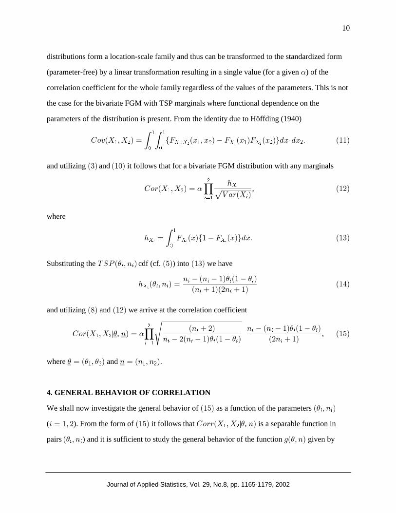
distributions form a location-scale family and thus can be transformed to the standardized form
(parameter-free) by a linear transformation resulting in a single value (for a given ) of the�
correlation coefficient for the whole family regardless of the values of the parameters. This is not
the case for the bivariate FGM with TSP marginals where functional dependence on the
parameters of the distribution is present. From the identity due to Höffding (1940)
*+,�� �� � � ' � �� �� �� �(/� /� �" # \ " \ # " #! !
" "� � � �� � � �\ Ä\ " #" # " #����
and utilizing and it follows that for a bivariate FGM distribution with any marginals��� ����
*+"�� �� � � �� !"�� �
" #
3æ"
#
3
�� �0\3 ,
where
0 � ���'� ���(/� ����\ \ \!
"
3 3 3� � � .
Substituting the cdf (cf. ) into we have#$%� � � � ��� �����3 3
0 � � � � � ����� �� �� �� �
�� ����� ��\ 3 3
3 3 3 3
3 33�
� �
and utilizing and we arrive at the correlation coefficient��� ����
*+"�� �� � � ����" #
3æ"
#
|�, � �� �� �� � �� �� �� �
� ��� �� �� � ��� ��3 3 3 3 3
3 3 3 3 3� �
� �,
where � � � � � � �� � � ��� �" # " # and �
4. GENERAL BEHAVIOR OF CORRELATION
We shall now investigate the general behavior of as a function of the parameters ���� � � � ��3 3
( ). From the form of it follows that � � �� � ���� *+""�� �� �" #| is a separable function in�, �
pairs ) and it is sufficient to study the general behavior of the function � � � 1�3 3 � � ��� given by

11
Journal of Applied Statistics, Vol. 29, No.8, pp. 1165-1179, 2002
1� � �� ��� �� '� �� �� �� �(
��� �� � ��� �� �� ��
� �
� �#
#
����
� � ��� �� �� �� �� �
��� �� �'� ��� �� �� �(#
# # # �� �
� �
to assess the effect of the marginals on the product moment correlation. Since 1� � ��� given by
���� coincides with the correlation of an FGM distribution with identical TSP marginals with
parameters , , and the dependence parameter the � � �3 3� � � � � � � �� � � �� extremes of
1� � �� � ����� coincide with extremes of the product moment correlation (cf ).
The first factor in is just ��� ������ ��# ���� the correlation between the power
marginals ( and determines the general behavior of the product moment correlation� � ��
coefficient as a function of . The second term in may be interpreted as a correction factor� ����
to account for increased symmetry in the TSP marginals relative to the skewed power marginals.
Since the variance is strictly positive and utilizing it follows that this correction factor is���
greater than for , . For both or the correction factor attains its� & ��� �� � 2 � � � � �� � �
minimum equal to and hence attains (for a fixed ) its minimum at� 1 � ��� ������ ��� � ��� #
either or . Writing� �� � � �
�� �� �� � �� ��
�'� ��� �� �� �(� �� � ����
���� ��
# # # #
8µ"� 
� �
� �� �
#
) )
it immediately follows that the correction factor is a strictly increasing function in the parameter
� � � � �� �� � 1� � �� ���� � �. This implies that (cf. ) attains its maximum for fixed at ."#
Taking the partial derivative in with respect to yields���� �
3 �� � ��� �� '� �� �� (
3� ��� �� '� ��� �� (1� � �� � �� �� � �����
� � �
�$ #
where as above . Since , Hence, noting that given� � � � � �� �� � & ��� �� & ��� �� 0 � � � �"% \ 3 33
by is strictly positive it follows from that for fixed is a strictly increasing���� ���� � 1� � ��� �
function of for and a strictly decreasing one for Hence for any fixed � � � � � � 4 �� � the

12
Journal of Applied Statistics, Vol. 29, No.8, pp. 1165-1179, 2002
function attains its maximum at . Since 1 � � � 1� � �� � � �� � ���� � we can conclude that the
product moment correlation of the FGM with TSP marginals attains its global maximum ���
when both TSP marginals are uniform. This agrees with the general result in Schucany et al.
(1978), already mentioned above, that the maximum correlation of an FGM distribution is
attained for uniform marginals. Also it follows from that for a fixed ,���� � � (and thus a fixed )
the minimal correlation is attained either when or . Utilizing we derive� 5 � � 6 7 ����
1 ��-�� � �� � 8�9 1� � �� � �� �� 5 �
� � � �
1 � ����� �7� � 8�9 1� � �� � � � 6 7
� �� �
� � � �� �� �
� �
� � # # �
Figures 4 summarize the extremes of the function 1� � �� ���� � as a function of the parameter
keeping ( ) fixed. Figure 4A focusses on the extremes of as a function of for values� 1� � ��� � �
of 1 and displays 1 (the global maximum) and (cf. ) (the minimal� � 1� � � � ��� 1� � �� ��-�� �
value of for fixed with 1). Analogously, Figure 4B focusses on the extremes of1� � �� � �� �
1� � �� � 4 � 1� � � � ��� 1� �7� ����� � � � as a function of for , displays 1 and (cf. ) (the minimal
value of for fixed with ). Figure 4C presents the extremes of as function1� � �� � 4 � 1� � ��� � �
of keeping fixed and displays the maximum for fixed ) and (the� 1� � �� � � 1��� �� � 1��� ��� "#
minimal value for fixed ). . Figures 4 A,� � � �� Figure 5 provides a three dimensional graph of 1 �
B and C may be interpreted as two-dimensional Figure 5 in various directions.:"+;<=>�+�? of
From and Figures 4 it follows that the correlation is bounded from above by the product����
moment correlation of the FGM distribution with uniform marginals and from below by���
� ���� ������ �� # the correlation of the FGM distribution with power marginals ,� � ��
or its reflection ( ). From Figures 4A and 4B it follows that for fixed and the� � � � �" #
correlation attains it maximal value when both TSP marginals are symmetric ( and its� � �"#
minimal value when both TSP marginals attain the maximal skewness ( ) Figure 4C� & '�� �( �
shows that the maximum discrepancy between the correlation with identical power marginals
with and identical TSP marginals with is equal to� � � � � �3 3

13
Journal of Applied Statistics, Vol. 29, No.8, pp. 1165-1179, 2002
/��� � 1� � �� 1��� �� � ����� � � � � �
� � � � �� � �#
.
Figure 4. The extremes of the function g(θ, n); A: as a function of θ ( 0 < n ≤ 1 ) ;B: as a function of θ ( n ≥ 1 ) ; C: as a function of n (θ ∈ [0,1] ).
0.00
0.05
0.10
0.15
0.20
0.25
0.30
0.35
0.00 0.25 0.50 0.75 1.00
0.00
0.05
0.10
0.15
0.20
0.25
0.30
0.35
0.00 1.00 2.00 3.00 4.00 5.00 6.00 7.00 8.00 9.00 10.00
0.00
0.05
0.10
0.15
0.20
0.25
0.30
0.35
0.00 0.25 0.50 0.75 1.00→ θ → θ
→ n
),2
1( ng
),0( ng
),( ∞θg
)1,(θg)1,(θg
)0,(θg
BA
C
0.00
0.05
0.10
0.15
0.20
0.25
0.30
0.35
0.00 0.25 0.50 0.75 1.00
0.00
0.05
0.10
0.15
0.20
0.25
0.30
0.35
0.00 1.00 2.00 3.00 4.00 5.00 6.00 7.00 8.00 9.00 10.00
0.00
0.05
0.10
0.15
0.20
0.25
0.30
0.35
0.00 0.25 0.50 0.75 1.00→ θ → θ
→ n
),2
1( ng
),0( ng
),( ∞θg
)1,(θg)1,(θg
)0,(θg
BA
C
The function describes, for fixed , the discrepancy in the correlation due to the/��� � maximum
skewness parameter ; it is a strictly decreasing (increasing) function of on ( )). For� � ��� �� ���7
� 6 7 /��� 6 � /�7� � � �, ( )and the largest discrepancy is attained at . Apparently (see"$#
Figure 4C) the difference between the correlations of FGM distributions with identical TSP
marginals and identical power marginals is the largest for small values of . However, for�
� � @ ���� ���� �� ���
��ø
�,
/�� � � /�7� � � � �ø ø"$# . Hence, for all values of (which are plausible in applications) the
discrepancy From it follows that Thus we have/��� � �������� ���� 1��� � � @ ��������"$#
ø

14
Journal of Applied Statistics, Vol. 29, No.8, pp. 1165-1179, 2002
reached the important conclusion that for varies from to (the� � � 1� � �� 1��� � � 1� � ��ø ø� �
uniform case) at most .@ � �������� @ �����-�"$
Figure 5. General behavior of function g(θ, n) given by (16) as a function of θ and n.
0 1 2 3 4 5 6 7 8 9 100.00
0.50
1.000.000
0.050
0.100
0.150
0.200
0.250
0.300
0.350
n θ
),( ng θ
0 1 2 3 4 5 6 7 8 9 100.00
0.50
1.000.000
0.050
0.100
0.150
0.200
0.250
0.300
0.350
n θ
),( ng θ
Summarizing the function for values of varies in the narrow range of1� � �� � � �� ø
@ �����-� from the correlation coefficient of an FGM distribution with uniform marginals.
Moreover, for fixed the correlation coefficient of an FGM with identical TSP marginals� � � �ø
is strictly larger than the correlation coefficient of an FGM with identical power marginals, but
differs from it by no more than for all values Hence, the effect of the"$# � ������� & ��� ����
parameters and on the value of the product moment correlation is almost negligible for� �
practical purposes. The general behavior of the product moment correlation with TSP marginals
closely follows the behavior of the FGM with power marginals, i.e. it increases for and� & ��� ��
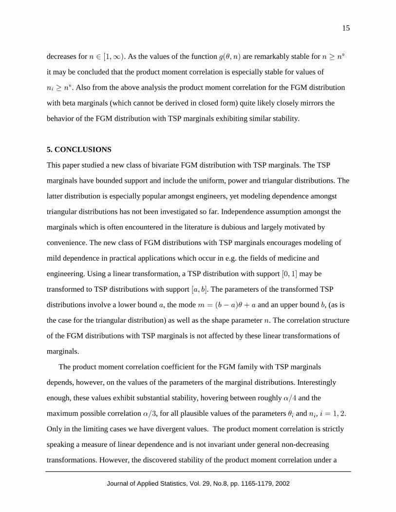
15
Journal of Applied Statistics, Vol. 29, No.8, pp. 1165-1179, 2002
decreases for . As the values of the function are remarkably stable for � & ���7� 1� � �� � 4 �� ø
it may be concluded that the product moment correlation is especially stable for values of
� 4 �3ø. Also from the above analysis the product moment correlation for the FGM distribution
with beta marginals (which cannot be derived in closed form) quite likely closely mirrors the
behavior of the FGM distribution with TSP marginals exhibiting similar stability.
5. CONCLUSIONS
This paper studied a new class of bivariate FGM distribution with TSP marginals. The TSP
marginals have bounded support and include the uniform, power and triangular distributions. The
latter distribution is especially popular amongst engineers, yet modeling dependence amongst
triangular distributions has not been investigated so far. Independence assumption amongst the
marginals which is often encountered in the literature is dubious and largely motivated by
convenience. The new class of FGM distributions with TSP marginals encourages modeling of
mild dependence in practical applications which occur in e.g. the fields of medicine and
engineering. Using a linear transformation, a TSP distribution with support may be��� ��
transformed to TSP distributions with support . The parameters of the transformed TSP�!� A�
distributions involve a lower bound , the mode and an upper bound , (as is! 9 � �A !� ! A�
the case for the triangular distribution) as well as the shape parameter . The correlation structure�
of the FGM distributions with TSP marginals is not affected by these linear transformations of
marginals.
The product moment correlation coefficient for the FGM family with TSP marginals
depends, however, on the values of the parameters of the marginal distributions. Interestingly
enough, these values exhibit substantial stability, hovering between roughly and the���
maximum possible correlation , for all plausible values of the parameters and , � ��� � � � �� ��3 3
Only in the limiting cases we have divergent values. The product moment correlation is strictly
speaking a measure of linear dependence and is not invariant under general non-decreasing
transformations. However, the discovered stability of the product moment correlation under a

16
Journal of Applied Statistics, Vol. 29, No.8, pp. 1165-1179, 2002
wide variety of marginals of diverse forms in the FGM distributions suggests that for bivariate
distributions with bounded support, this coefficient also is a suitable measure of positive (or
negative) dependence. An extension of these results to generalized FGM distributions (with
larger correlation coefficients) could be of some interest and utility.
6. REFERENCES
��������� (1985) The bivariate exponential distribution; A review and some new results,
Statistica Neerlandica, , 39 pp. 342-357.
��� ������������������������������� (2000) Reliability modeling, prediction,
and optimization, Wiley, New York.
���������������������������� (1998) Do our current assessments assure competency
in clinical breast evaluation results? 175, 6, pp. 497-The American Journal of Surgery,
502.
��������������� ����� (1986) Generalized Burr-Pareto-logistic distribution with
application to uranium exploration data set, 28, pp. 123-131.Technometrics,
�! ������ (1981) A Morgenstern-type bivariate gamma distribution, 68, 1,Biometrika,
pp. 339-440.
������������"��#��$ (2001) Imperial Press Singapore.Correlation and Dependence, ,
%���������� (1960) The performance of some correlation coefficients for a general bivariate
distribution, 47, pp. 307-323.Biometrika,
��&����� � (1960) Bivariate exponential distributions, Journal of the American Statistical
Association, 55, pp. 698-707.
���� ���������������� (1986) The joy of copulas, bivariate distributions with uniform
marginals, 40, 4, pp. 280-283.The American Statistician,
'())*������ (1940) Maszstabinvariante korrelationstheorie, Univ. Berlin, Schr. Math.
angew. Math., 5 (3), pp. 181-233.

17
Journal of Applied Statistics, Vol. 29, No.8, pp. 1165-1179, 2002
����+��,��" (1984) Measures of dependence, 4, Elsevier, NorthHandbook of Statistics,
Holland, pp. 79-88.
���� ������ (1997) The triangular distribution as a proxy for the beta distribution in risk
analysis, The Statistician, 46, No. 3, pp. 387-398.
���� �����-���"��#��$ (1975) On some generalized Farlie-Gumbel-Morgenstern
distribution, Communications in Statistics. 4, pp. 415-27.
���� �����-���"��#��$ (1977) On some generalized Farlie-Gumbel-Morgenstern
distribution - II: Regression, correlation and further generalization, Communications in
Statistics. 6, pp. 485-496.
���� �����-���"��#��$ (1999) Non-smooth sailing or triangular distributions revisited
after some 50 years, The Statistician, 48, Part 2, pp. 179-187.
���� �����-���"��#��$ (2001) Cloning of Distributions, submitted to .Statistics
"��#��$��������� �������������� �����- (2000) Continuous Multivariate
Distributions, Volume 1: Models and Applications, 2nd edition, Wiley, New York.
-����..�������$ (1984) Bivariate gamma distribution as a life test model, Aplikace
Matematiky, . 29� pp 182 - 188.
������ ������� (1956) Einfache beispiele zweidimensionaler verteilungen, Mitt. Math.
Statis. , 8, 234-235.
$�������������������������������� (1978) Correlation structure in Farlie-
Gumbul-Morgenstern distributions, 65, pp. 650-653.Biometrika,
������.�������"��#��$ (2002a) The Standard Two Sided Power Distribution and its
Properties: with Applications in Financial Engineering, 56, 2, The American Statistician,
90-99.
������.�������"��#��$ (2002b) A Novel Extension of the Triangular Distribution and
its Parameter Estimation, The Statistician, 51, 1-17.

18
Journal of Applied Statistics, Vol. 29, No.8, pp. 1165-1179, 2002
������.��������##������/0��%��������� ������������-� (1996) A Bayes�
approach to step-stress accelerated life testing, 45, 3,IEEE Transactions on Reliability,
491-498.