A. Velazquez, N.Clerbaux et al. Status of the BBR LW ......A. Velazquez, N.Clerbaux et al. Introduction The EarthCARE mission BBR Con guration Flux conversion algorithms Future work

A. Velazquez,N.Clerbaux et al.

Introduction

Flux conversionalgorithms

Future work

Status of the BBR LW Radiance to FluxBaseline conversion algorithm

A. Velazquez Blazquez, N. Clerbaux, A. Ipe, E. Baudrez, I.Decoster, S. Nevens, S. Dewitte (RMIB)

Royal Meteorological Institute of Belgium (RMIB)Vrije Universiteit Brussel(VUB)

Earth Radiation Budget Workshop 2012GFDL, Princeton, NJ. 22 - 25 October 2012


Introduction


Future work

Outline

IntroductionThe EarthCARE missionBBR Configuration

Flux conversion algorithmsSpectral modelValidation3-views flux estimation

Future work


Introduction

The EarthCAREmission

BBR Configuration


Future work

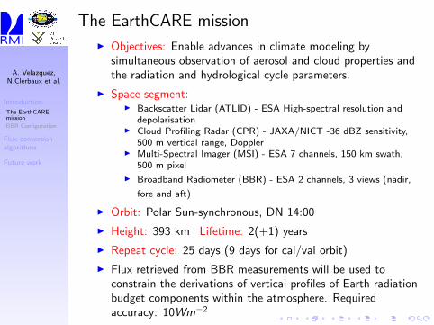
The EarthCARE mission

I Objectives: Enable advances in climate modeling bysimultaneous observation of aerosol and cloud properties andthe radiation and hydrological cycle parameters.

I Space segment:I Backscatter Lidar (ATLID) - ESA High-spectral resolution and

depolarisationI Cloud Profiling Radar (CPR) - JAXA/NICT -36 dBZ sensitivity,

500 m vertical range, DopplerI Multi-Spectral Imager (MSI) - ESA 7 channels, 150 km swath,

500 m pixel

I Broadband Radiometer (BBR) - ESA 2 channels, 3 views (nadir,

fore and aft)

I Orbit: Polar Sun-synchronous, DN 14:00

I Height: 393 km Lifetime: 2(+1) years

I Repeat cycle: 25 days (9 days for cal/val orbit)

I Flux retrieved from BBR measurements will be used toconstrain the derivations of vertical profiles of Earth radiationbudget components within the atmosphere. Requiredaccuracy: 10Wm−2


Introduction

The EarthCAREmission

BBR Configuration


Future work

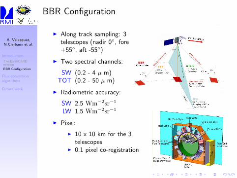
BBR Configuration

I Along track sampling: 3telescopes (nadir 0◦, fore+55◦, aft -55◦)

I Two spectral channels:

SW (0.2 - 4 µ m)TOT (0.2 - 50 µ m)

I Radiometric accuracy:

SW 2.5 Wm−2sr−1

LW 1.5 Wm−2sr−1

I Pixel:

I 10 x 10 km for the 3telescopes

I 0.1 pixel co-registration


Introduction


Spectral model

Validation

3-views fluxestimation

Future work

Flux conversion algorithms

Two different algorithms will be developed:

1. Baseline Flux Retrieval Algorithm ⇒ to obtain fluxaccuracies consistent with those of current ERBmissions (GERB, CERES, ScaRaB)

I Flux estimate for a single viewI Weighting of the viewsI Estimation of the reference level

2. Advanced Flux Retrieval Algorithm ⇒ to fullfill ECaccuracy requirements


Introduction


Spectral model

Validation


Future work

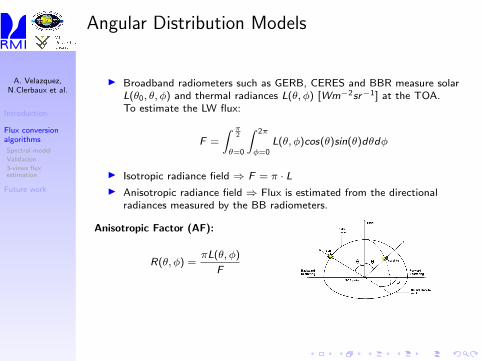
Angular Distribution Models

I Broadband radiometers such as GERB, CERES and BBR measure solarL(θ0, θ, φ) and thermal radiances L(θ, φ) [Wm−2sr−1] at the TOA.To estimate the LW flux:

F =

∫ π2

θ=0

∫ 2π

φ=0L(θ, φ)cos(θ)sin(θ)dθdφ

I Isotropic radiance field ⇒ F = π · LI Anisotropic radiance field ⇒ Flux is estimated from the directional

radiances measured by the BB radiometers.

Anisotropic Factor (AF):

R(θ, φ) =πL(θ, φ)

F


Introduction


Spectral model

Validation


Future work

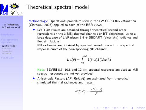
Theoretical spectral model

Methodology: Operational procedure used in the LW GERB flux estimation(Clerbaux, 2003) applied to each of the BBR views.

I LW TOA Fluxes are obtained through theoretical second orderregressions on the 3 MSI thermal channels or BT differences, using alarge database of LibRadtran 1.4 + SBDART (clear sky) radiance andflux simulations.NB radiances are obtained by spectral convolution with the spectralresponse curve of the corresponding NB channel:

Lnb(θ) =

∫ inf

0L(θ, λ)S(λ)d(λ)

Note: SEVIRI 8.7, 10.8 and 12 µm spectral responses are used as MSIspectral responses are not yet provided.

I Anisotropic Factors (AF, R(θ, φ)) are estimated from theoreticalsimulated thermal radiances and fluxes.

R(θ, φ) =πL(θ, φ)

F


Introduction


Spectral model

Validation


Future work

RT-based geophysical datasetsSITS LibRadtran database improved for warm scenes (270)

I 12096 thermal (LW) simulations, 540 are clear skyI Outputs at: 18 VZA: 0◦ to 85◦, step 5◦

I ASTER surface emissionI OPAC aerosol definitionI Standard atmospheric profiles + wv scaledI Cloud properties from Yang parametrizationI Fine spectral resolution

I LW sim: 2.5 to 100 µm (762 λ) + extended up to 500 µmI 2.5 to 14 µm, step of 0.05 µmI 14.1 to 50 µm, step of 0.1 µmI 55 to 100 µm, step of 0.5 µm

I Surface Temperature from profile + ∆T

SBDART databaseI 4622 thermal (LW) simulations, only used clear sky ones (2311)I Outputs at: 18 VZA: 0◦ to 85◦, step 5◦

I Atmospheric profiles from TIGR-3 databaseI Fine spectral resolutionI LW sim: 2.5 to 100 µm (431 λ) + extended up to 500 µmI Emissivity generated randomly between 0.85 and 1I Surface Temperature generated randomly with values close to the lowest

in the atmospheric profile


Introduction


Spectral model

Validation


Future work

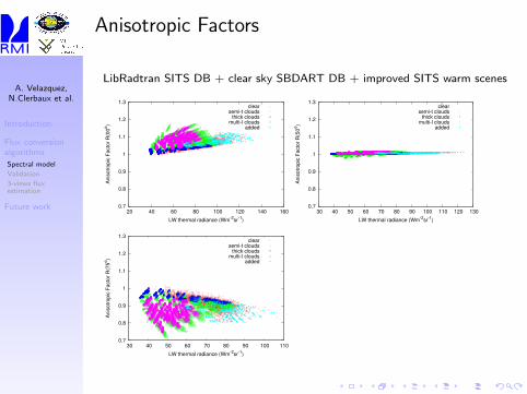
Anisotropic Factors

LibRadtran SITS DB + clear sky SBDART DB + improved SITS warm scenes

0.7

0.8

0.9

1

1.1

1.2

1.3

20 40 60 80 100 120 140 160

Anis

otr

opic

Facto

r R

(00

o)

LW thermal radiance (Wm-2

sr-1

)

clearsemi-t clouds

thick cloudsmulti-l clouds

added

0.7

0.8

0.9

1

1.1

1.2

1.3

30 40 50 60 70 80 90 100 110 120 130

Anis

otr

opic

Facto

r R

(50

o)


sr-1

)

clearsemi-t clouds


added

0.7

0.8

0.9

1

1.1

1.2

1.3

30 40 50 60 70 80 90 100 110

Anis

otr

opic

Facto

r R

(75

o)


sr-1

)

clearsemi-t clouds


added


Introduction


Spectral model

Validation


Future work

Anisotropy Models

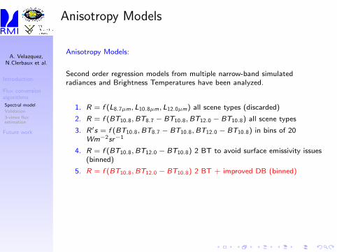
Anisotropy Models:

Second order regression models from multiple narrow-band simulatedradiances and Brightness Temperatures have been analyzed.

1. R = f (L8.7µm, L10.8µm, L12.0µm) all scene types (discarded)

2. R = f (BT10.8,BT8.7 − BT10.8,BT12.0 − BT10.8) all scene types

3. R′s = f (BT10.8,BT8.7 − BT10.8,BT12.0 − BT10.8) in bins of 20Wm−2sr−1

4. R = f (BT10.8,BT12.0 − BT10.8) 2 BT to avoid surface emissivity issues(binned)

5. R = f (BT10.8,BT12.0 − BT10.8) 2 BT + improved DB (binned)


Introduction


Spectral model

Validation


Future work

Validation strategy

I Validation database

In order to test the models for the radiance to flux conversion, avalidation database of collocated BBR-like and CERES SSF-Ed2B FM1,FM2, FM3, FM4 data for March and September 2004 has been built.

I ≈ 240 millions of CERES and SEVIRI pairs over theSEVIRI disk

I BBR BB radiances obtained from the conversion fromNB SEVIRI radiances to GERB BB radiances usingknown coef for GERB.

I angular model for the BBR applied to BBR BBradiances to obtain BBR flux.

I Apply theoretical ADM’s to CERES night time data

Similar ADM’s developed using MODIS 11.03 and 12.02 channels areapplied to CERES night time BB radiances and then compared withCERES Fluxes


Introduction


Spectral model

Validation


Future work

Validation strategy

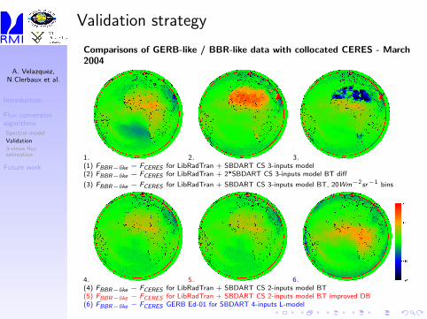
Comparisons of GERB-like / BBR-like data with collocated CERES - March2004

1. 2. 3.(1) FBBR−like − FCERES for LibRadTran + SBDART CS 3-inputs model(2) FBBR−like − FCERES for LibRadTran + 2*SBDART CS 3-inputs model BT diff

(3) FBBR−like − FCERES for LibRadTran + SBDART CS 3-inputs model BT, 20Wm−2sr−1 bins

4. 5. 6.(4) FBBR−like − FCERES for LibRadTran + SBDART CS 2-inputs model BT(5) FBBR−like − FCERES for LibRadTran + SBDART CS 2-inputs model BT improved DB(6) FBBR−like − FCERES GERB Ed-01 for SBDART 4-inputs L-model


Introduction


Spectral model

Validation


Future work

Validation strategy

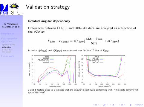
Residual angular dependency

Differences between CERES and BBR-like data are analyzed as a function ofthe VZA as:

FBBR − FCERES = a(FBBR)52.5− θBBR

52.5+ b(FBBR)

In which a(FBBR ) and b(FBBR ) are estimated over 20 Wm−2 bins of FBBR .

-10

-5

0

5

10

15

20

25

30

50 100 150 200 250 300 350 400

Nadir e

rror

(a)

[W

/m2]

Thermal flux [W/m2]

BBR 3BBR 3 BT

BBR 3 BT (10*hot)BBR 3 BT (bins)

BBR 2 BT

-10

-5

0

5

10

15

20

25

30

50 100 150 200 250 300 350 400

Off-n

adir e

rror

(b)

[W

/m2]

Thermal flux [W/m2]

BBR 3BBR 3 BT

BBR 3 BT (10*hot)BBR 3 BT (bins)

BBR 2 BT

a and b factors close to 0 indicate that the angular modelling is performing well. All models perform wellup to 280 Wm2.


Introduction


Spectral model

Validation


Future work

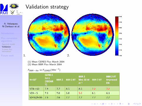
Validation strategy

1. 2.

(1) Mean CERES Flux March 2004(2) Mean BBR Flux March 2004

FBBR−like vs FCERES (Wm−2)

Errors consistent with 2% differences between GERB and CERES


Introduction


Spectral model

Validation


Future work

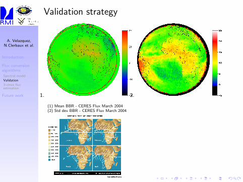
Validation strategy

1. 2.

(1) Mean BBR - CERES Flux March 2004(2) Std dev BBR - CERES Flux March 2004


Introduction


Spectral model

Validation


Future work

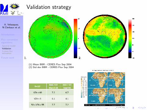
Validation strategy

1. 2.

(1) Mean BBR - CERES Flux Sep 2004(2) Std dev BBR - CERES Flux Sep 2004


Introduction


Spectral model

Validation


Future work

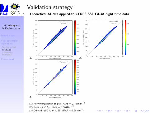
Validation strategyTheoretical ADM’s applied to CERES SSF Ed-3A night time data

1.0

50

100

150

200

250

300

350

400

AD

M s

imu

late

d L

W F

lux

[W

/m2]

0 50 100 150 200 250 300 350 400

CERES LW Flux[W/m2]

10000

20000

30000

40000

50000

60000

70000

80000N=15236794

RMS=2.745788 W/m2

2.0

50

100

150

200

250

300

350

400

AD

M s

imu

late

d L

W F

lux

[W

/m2]

0 50 100 150 200 250 300 350 400

CERES LW Flux[W/m2]

2500

5000

7500N=1277942

RMS=3.531226 W/m2

3.0

50

100

150

200

250

300

350

400

AD

M s

imu

late

d L

W F

lux

[W

/m2]

0 50 100 150 200 250 300 350 400

CERES LW Flux[W/m2]

2500

5000

7500

10000

12500

15000

17500

20000

22500

25000

27500

30000

32500

35000

N=3414258

RMS=0.973385 W/m2

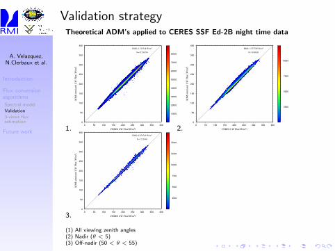
(1) All viewing zenith angles. RMS = 2.75Wm−2

(2) Nadir (θ < 5). RMS = 3.56Wm−2

(3) Off-nadir (50 < θ < 55).RMS = 0.98Wm−2


Introduction


Spectral model

Validation


Future work

Validation strategyTheoretical ADM’s applied to CERES SSF Ed-2B night time data

1.0

50

100

150

200

250

300

350

400

AD

M s

imu

late

d L

W F

lux

[W

/m2]

0 50 100 150 200 250 300 350 400

CERES LW Flux[W/m2]

10000

20000

30000

40000

50000

60000

70000

80000N=15236794

RMS=2.745548 W/m2

2.0

50

100

150

200

250

300

350

400

AD

M s

imu

late

d L

W F

lux

[W

/m2]

0 50 100 150 200 250 300 350 400

CERES LW Flux[W/m2]

2500

5000

7500

10000

N=1938920

RMS=3.557789 W/m2

3.0

50

100

150

200

250

300

350

400

AD

M s

imu

late

d L

W F

lux

[W

/m2]

0 50 100 150 200 250 300 350 400

CERES LW Flux[W/m2]

2500

5000

7500

10000

12500

15000

N=1725948

RMS=0.976769 W/m2

(1) All viewing zenith angles(2) Nadir (θ < 5)(3) Off-nadir (50 < θ < 55)


Introduction


Spectral model

Validation


Future work

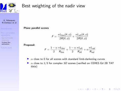
Best weighting of the nadir view

Plane parallel scenes

F =πLfore(θ, φ)

2R(θ, φ)+πLaft(θ, φ)

2R(θ, φ)

Proposal:

F =1− α

2

πLfore

Rfore+

1− α2

πLaft

Raft+ α

πLrad

Rrad

I α close to 0 for all scenes with standard limb-darkening curves

I α close to 1/3 for complex 3D scenes (verified on CERES Ed 2B TATdata)


Introduction


Spectral model

Validation


Future work

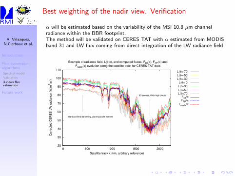
Best weighting of the nadir view. Verification

α will be estimated based on the variability of the MSI 10.8 µm channelradiance within the BBR footprint.The method will be validated on CERES TAT with α estimated from MODISband 31 and LW flux coming from direct integration of the LW radiance field

20

30

40

50

60

70

80

90

100

110

0 500 1000 1500 2000

Corr

ecte

d C

ER

ES

LW

radia

nce (

W/m

2/s

r)

Satellite track x (km, arbitrary reference)

Example of radiance field, L(θ,x), and computed fluxes, FDI(x), FPP(x) and

Fnadir(x) evolution along the satellite track for CERES TAT data

standard limb darkening, plane-parallel scenes

3D scenes, thick high clouds

L(θ=-70)

L(θ=-50)

L(θ=-30)

L(θ= 0)

L(θ=30)

L(θ=50)

L(θ=70)FDI/π

FPP/π

Fnadir/π


Introduction


Future work

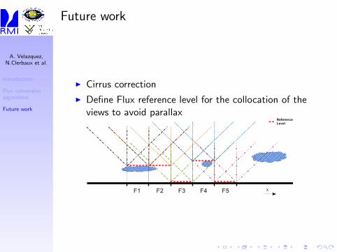
Future work

I Cirrus correction

I Define Flux reference level for the collocation of theviews to avoid parallax

� �

��

��

��

Documents

A. Velazquez, N.Clerbaux et al. Status of the BBR LW ......A. Velazquez, N.Clerbaux et al. Introduction The EarthCARE mission BBR Con guration Flux conversion algorithms Future work