A variational form ulation for Þ nite deform ation w … · w rinkling analysis of inelastic m em branes J.M osler M aterials M echanics Institute for M aterials R esearch G K SS

A variational formulation for finite deformationwrinkling analysis of inelastic membranes

J. Mosler

Materials MechanicsInstitute for Materials ResearchGKSS Research CentreD-21502 Geesthacht, GermanyE-Mail: [email protected]

F. Cirak

Department of EngineeringUniversity of CambridgeTrumpington StreetCambridge, CB2 1PZ, United KingdomE-Mail: [email protected]

SUMMARY

This paper is concerned with a novel, fully variational formulation for finite deformation analysis of in-elastic membranes with wrinkling. In contrast to conventional approaches, every aspect of the physicalproblem derives from minimization of suitable energy functionals. A variational formulation of finitestrain plasticity theory, which leads to a minimization problem for the constitutive updates, serves asthe starting point for the derivations. In order to take into account the kinematics induced by wrinklesand slacks, a relaxed version of the finite strain functional is postulated. In effect, the local incremen-tal stress-strain relations are established via differentiation of the relaxed energy functional with respectto the strains. Hence, the presented formulation is fully analogous to that of hyperelasticity with thesole exception that the aforementioned functional depends on history variables and, accordingly, it ispath dependent. The advantages associated with the developed variational method are manifold. Froma practical point of view, the possibility of applying standard optimization algorithms to solve the mini-mization problem describing inelastic membranes is remunerative. From a mathematical point of view,on the other hand, the energy of the system induces some sort of natural metric representing an essentialrequirement for error estimation and thus, for adaptive finite element methods. The presented derivationof the model allows to consider possible material symmetries in the elastic as well as plastic response ofthe material. As a prototype, a von Mises-type model is implemented. The efficiency and performanceof the resulting algorithm are demonstrated by means of numerical examples.

1 IntroductionMembranes are ubiquitous structural members in a number of engineering applications rangingfrom light-weight roofs in civil engineering, airbags in automobiles, solar sails and sunshieldsin aerospace engineering to stents in bio-engineering. Although the listed applications are rel-atively new, mechanical models for membranes go at least back to the works of Wagner [1]and Reissner [2] in the 30s. In [1, 2] it is assumed that the membrane has no bending stiffnessand, hence, cannot carry compressive stresses. This assumption leads directly to the celebratedtension field theory by Wagner, which has been elaborated upon by a number of researchers,cf., e.g. [3–9]. A comprehensive overview of the work carried out on tension field theory priorto 1990 can be found in [10] and references cited therein.

Despite the considerable success of the classical tension field theory in analytical case-by-case investigation and computational analysis of membranes structures, its numerical imple-mentation is not straightforward. In particular for finite deformations, it leads to ambiguities

1

cirak

Sticky Note

Draft version. Final version published in Computer Methods in Applied Mechanics and Engineering Comput, 198(27-29):2087–2098, 2009.

2 J. MOSLER & F. Cirak

with respect to the loading and unloading conditions, or in other terms, the wrinkling criteria.More precisely, once wrinkling occurs, the resulting stress field can indeed be computed byapplying tension field theory, however, the theory does not provide any information if such awrinkle forms. Hence, an additional criterion is needed, which is usually based on principalstrains, principal stresses or a combination of both, cf. [7, 8]. Clearly, since these loadingconditions are often introduced in ad-hoc manner, there is no guarantee that they comply wellwith the tension field theory. As a consequence, the resulting boundary value problem is notcontinuous in general. Evidently, this is not physical and gives rise to numerical problems aswell.

Alternatively, a fully variational strategy suitable for the analysis of wrinkles and slacksin membranes was proposed in a series of papers by Pipkin, cf. [11–13], see also [14]. Pip-kin analyzed the energy of a membrane under certain assumptions and proved that the quasi-convexification of the Helmholtz energy defines a relaxed energy functional whose derivativesyield the membrane stresses, i.e., the stresses predicted by this relaxed potential fulfill the re-strictions imposed by tension field theory. Interestingly, and in contrast to classical tension fieldtheory, Pipkin’s method inherently includes physically sound loading and unloading conditions;additional ad-hoc assumptions are not necessary. As a consequence, the resulting boundaryvalue is continuous (more precisely, sufficiently smooth), which makes it physically and math-ematically sound and convenient for numerical implementations.

Pipkin’s ideas were further elaborated on by Mosler [15] in which a novel variational algo-rithmic formulation for wrinkling at finite strains was proposed. In line with Pipkin’s originalwork [11–13], the unknown wrinkle distribution is computed by minimizing the Helmholtz en-ergy of the membrane with respect to the wrinkling parameters. The finite element model [15]allows to employ arbitrary, fully three-dimensional hyperelastic constitutive models directly.Furthermore, the plane stress conditions characterizing a membrane stress state are naturallyincluded within the variational formulation.

In the present paper, the method advocated by Mosler [15] is extended to inelastic mem-branes. Although the ability to predict the deformations and ultimate load capacity of plas-tically deforming membranes is important, for example, for inflatable ETFE (Ethylene TetraFluoro Ethylene) cushions used in architecture [16] or sheet metal forming [17, 18], only fewnumerical methods have been proposed yet, cf. [19, 20]. In contrast to the cited references,the approach developed in this paper is fully variational, i.e., the wrinkling parameters, togetherwith the plasticity related variables, follow from relaxing an incrementally defined potential andthe stresses are computed simply by differentiating this functional. Thus, the relaxed potential isformally identical to that of standard hyperelasticity. Clearly, such a variational method showsseveral advantages compared to conventional strategies. For instance, it opens up the possibilityof applying standard optimization algorithms to the numerical implementation, see [15]. This isespecially important for highly non-linear or singular problems such as wrinkling. On the otherhand, minimization principles provide a suitable basis for a posteriori error estimation and thus,for adaptive finite element formulations, cf. [21–23].

The paper is organized as follows: In Section 2, the fully variational wrinkling model pro-posed in [15] is briefly summarized. For the sake of simplicity, focus is on hyperelastic ma-terials. Subsequently, a variational framework for finite strain plasticity theory is discussed inSection 3. In line with the wrinkling model, it allows to reformulate the elastoplastic constitu-tive update as a minimization problem. The key contribution of the present paper is elaboratedin Section 4. More precisely, the minimization principles for wrinkling in elastic membranesand for plasticity in inelastic solids are combined to a novel variational approach for inelas-tic membranes. The performance of the resulting algorithmic formulation is demonstrated inSection 5.

Variational formulation for wrinkling in inelastic membranes 3

2 Wrinkling in (hyper)elastic membranesIn this section, a summary of the variational formulation for wrinkling at finite strains basedon energy minimization is presented. While Subsection 2.1 is concerned with the kinematicsinduced by slacks and wrinkles, details on the resulting variational strategy are given in Sub-section 2.2. Further details may be found in the reference [15].

2.1 KinematicsIn the following, a membrane in its reference undeformed configuration is considered. Since amembrane represents a two-dimensional submanifold in the three-dimensional space, it can beconveniently characterized by an atlas. Hence, the reference configuration ! ! R3 is (locally)defined by a chart X : R2 " U #! M ! R3, !! $# X . The same concept can be applied tothe description of the deformed configuration !(!), i.e., x : R2 " U #! K ! R3, !! $# xwith X and x being the position vectors of a point within the undeformed and the deformedconfiguration, respectively. Assuming that the charts are sufficiently smooth diffeomorphisms,the deformation mapping ! connecting X and x is well defined, i.e., ! = x % X

!1 and thedeformation gradient yields F := "x/"!! & "!!/!X . Based on F the right Cauchy-Greenstrain tensor C = F T · F can be computed. C is a symmetric (C = CT ) and positive definite(C > 0) second-order tensor. It is noteworthy that for membranes, the deformation gradient Fas well as the strain tensor C can be represented by 2 ' 2 tensors without loss of generality,despiteM ! R3 and K ! R3, cf. [6, 12]. However, since in this paper fully three-dimensionalconstitutive models will be considered, a three-dimensional strain state is required. Using thespectral decomposition theorem, C can be written in the following form:

C = (#C1 )2 N 1 & N 1 + (#C

2 )2 N 2 & N 2 + (#C3 )2 N 3 & N 3, (1)

where the orthogonal unit eigenvectorsN 1 andN 2 are in the tangent space of the undeformedmembrane surface while the unit vectorN 3 is normalN 1 andN 2. Thereby, it is assumed thatthe out-of-plane shear strains of the membrane are zero.

So far, the kinematics induced by wrinkles have not been taken into account. In general,wrinkling can either be modeled explicitly using thin shell models [24], or in a smeared fashion[15]. Here, the focus is on the latter approach which is particularly useful in presence of finewrinkling. More precisely, the additional out-of-plane component of the deformation mappingdue to wrinkles is captured by a right Cauchy-Green tensor Cw. Consequently, the effective orrelaxed strain tensorCr reads

Cr = C + Cw. (2)As shown in [13, 15, 20], the wrinkling-related part Cw can be decomposed according to

Cw = a2 N & N (3)

withN being the wrinkling direction and the scalar a depends on the frequency and amplitudesof the wrinkles. According to Eq. (3), Cw is semi-positive definite (Cw ( 0) and hence,Cr > 0.

If wrinkles and slacks are to be modeled, a slight modification of the kinematics is necessary.Conceptionally, slacks can be understood as two orthogonal wrinkles which lead to

Cw = a2 N & N + b2 M & M , (4)

cf. [15]. Here, the orthogonal vectors N and M span the tangent space of the undeformedmembrane. Obviously,Cw is identical to Eq. (3), if b equals zero. Otherwise, Cw corresponds


to a slack. Interestingly, if Cw is interpreted as a 2 ' 2 tensor (within the tangent space of!), any symmetric semi-positive definite tensor can be generated by varying a, b and N . As aresult, the relaxed strain tensor can be re-written as

Cr = C + Cw, Cw ( 0, (5)

cf. [13]. Again,Cw ( 0 denotes thatCw is semi-positive definite.

2.2 A variational formulation for wrinkling at finite strains based on en-ergy minimization

For the sake of clarity, attention is focused on wrinkling in (hyper)elastic materials first. In thiscase, a strain energy functional " = "(C) exists and the first Piola-Kirchhoff stress tensor Pand the second Piola-Kirchhoff stresses S are computed as

P = 2 F ·""

"CS = 2

""

"C. (6)

Furthermore, it is assumed that the reference configuration is stress free (locally), i.e.,

"(C = 1) = 0, P (C = 1) = 0. (7)

It is well known that for such material models the deformation mapping ! can be computed byapplying the principle of minimum potential energy, i.e.,

! = arg inf!

I(!), (8)

withI(!) :=

!

!

"(C) dV )!

!

B · ! dV )!

"!2

T · ! dA. (9)

Here, B and T represent prescribed body forces and tractions acting on "!2. Obviously, !has to comply with the essential boundary conditions imposing additional restrictions in theresulting minimization problem. Clearly, if principle (8) is directly employed, physically inad-missible compressive membrane stresses may occur.

According to the previous subsection, wrinkles or slacks can be taken into account by mod-ifying the right Cauchy-Green tensor. Thus, the potential energy of a membrane is given simplyby replacing the standard strain tensor C in Eq. (9) by its relaxed counterpart, cf. Eq. (2).Denoting now the deformation of the middle plane of the membrane as !, the energy of ahyperelastic membrane reads

I(!, #C3 , a, b, $) :=

!

!

"(Cr(!, #C3 , a, b, $)) dV )

!

!

B · ! dV )!

"!2

T · ! dA. (10)

In Eq. (10), $ represents an angle which defines the vectors N = [cos $; sin $]T and M =[) sin $; cos $]T (the normal vector N 3 is known in advance). Since energy minimization isthe overriding principle governing every aspect of the mechanical problem under investigation,it is natural to postulate that wrinkles and slacks form such that they lead to the energeticallymost favorable state:

(!, #C3 , a, b, $) = arg inf

!,#C3 ,a,b,!

I(!, #C3 , a, b, $). (11)


Since the variables a, b, $ and #C3 are locally defined, the minimization problem (11) can

be decomposed into two consecutive optimization problems. First, for a given deformationmapping, the parameters a, b, $ and #C

3 are computed from the local minimization problem

(#C3 , a, b, $) := arg inf

#C3 ,a,b,!

"(!, #C3 , a, b, $) (12)

which defines a relaxed energy functional

"r(C(!)) = inf#C3 ,a,b,!

"(!, #C3 , a, b, $) (13)

depending only on the deformation mapping. It can be shown that the stationarity conditionsassociated with the minimization problem (12) are given by

""

"#C3

= 0 *+ #C3 S33 = 0 *+ %33 = 0

""

"a= 0 *+ a SNN = 0 *+ SNN = 0 (if a ,= 0)

""

"b= 0 *+ b SMM = 0 *+ SMM = 0 (if b ,= 0)

""

"$= 0 *+ (a2 ) b2) SNM = 0 *+ SNM = 0 (if a ,= 0 or b ,= 0),

(14)

cf. [15]. Here, " are the Cauchy stresses and SNN := S : (N&N ), SNM := S : (N&M ) andSMM := S : (M & M) with the second Piola-Kirchhoff stresses S = 2 "Cr

". Accordingly,plane stress conditions are naturally included within the variational formulation (note that theout-of-plane shear strains vanish). Furthermore, in case of wrinkling (a ,= 0, b = 0), theresulting stress state is one-dimensional, i.e., SNN = 0, SNM = 0, while the stresses vanishcompletely, if a slack forms. Further details of the stationary conditions (14) the can be foundin [15].

Once the local problem (13) has been solved, the deformation mapping follows from thefollowing minimization problem on the structure level:

! = arg inf!

"

#

!

!

"r(C) dV )!

!

B · ! dV )!

"!2

T · ! dA

$

% . (15)

It bears emphasis that both problems (12) and (15) can be computed by using standard op-timization algorithms. For the spatial discretization of Eq. (15) the finite element method isused.Remark 1. Wrinkles or slacks form, if they are energetically favorable. They result from thelocal minimization problem (12). The respective stationarity conditions are summarized inEqs. (14). According to [15], the associated wrinkling conditions can be computed from a trialstate characterized by vanishing slacks and wrinkles, i.e.,Cr = C. More precisely:

• S ( 0 + no wrinkles or slacks• (#C

1 )2 > 1, (#C2 )2 < (#C

1 )2, S(C) ,( 0 + wrinkling• (#C

1 )2 < 1, (#C2 )2 < 1 + slack + Cr = 1, + S = 0, " = 0

Here, S ( 0 is used to signal that S is semi-positive definite, i.e., the eigenvalues are not lessthan zero.


Remark 2. If " is an isotropic tensor function, the minimization problem (12) can be solvedsemi-analytically. More precisely, a variation with respect to the wrinkling parameters a and byieldsM = N 1 andN = N 2 with #C

1 > #C2 . Hence,C andCw are coaxial and the wrinkling

directions are known in advance. Furthermore, in case of wrinkling (no slacks), the resultingstress state is one-dimensional and hence, two of the eigenvalues ofCr are identical (#C

2 = #C3 ).

Consequently, the minimization problem (12) depends only on a, i.e., it is scalar-valued.

3 Variational constitutive updatesThis section is concerned with the so-called variational constitutive updates. Those updatesallow to formulate a broad range of different plasticity or damage models as optimization prob-lems similar to that of wrinkling (compare to Eq. (11)). As a prototype and for the sake ofconcreteness, attention is restricted to finite strain plasticity theory based on a multiplicativedecomposition of the deformation gradient into elastic F e and plastic F p parts (F = F e · F p).Evidently, for path-dependent problems such as plasticity theory, the optimization problem isdefined pointwise (with respect to the (pseudo) time). Throughout this section, the kinematicsinduced by wrinkles or slacks are not taken into account. The coupling of variational constitu-tive updates and the variational wrinkling algorithm in Section 2 will be discussed in Section 4.This section follows to a large extend the previous works [25–27]. An overview on the slightlydifferent variational constitutive updates which can be found in the literature is given in [22].

3.1 FundamentalsFocusing on plasticity models, the Helmholtz energy reads

"(F , F p, #) = "e(F e) +"p(#) (16)

with # being internal strain-like variables. While "e represents the elastic stored energy, thesecond term in Eq. (16) denotes the stored energy due to plastic work. It is associated withisotropic/kinematic hardening/softening. In case of so-called standard dissipative solids in thesense of Halphen & Nguyen [28], which are the cornerstone of variational constitutive updates,the material model is completely defined by means of only two scalar-valued functions. One ofthose is the Helmholtz energy, while the other, namely the yield function &, spans the admissiblestress space E$ , i.e.,

E$ := {(!, Q) - R9"n | & = &(!, Q) . 0}, Q := )""". (17)

Here,! are the Mandel stresses andQ is a set of n internal stress-like variables conjugate to #.Assuming associativity, the flow rules and the evolution equations are obtained as

Lp := Fp · F p!1 = # "!&

&'()

=: K

, # = # "Q&. (18)

The plastic multiplier # in Eq. (18) has to fulfill the Karush-Kuhn-Tucker conditions

# ( 0, & . 0, # & = 0. (19)

For the derivation of variational constitutive updates, the potential

E(!, Fp, #,!, Q) = "(!, F

p, #) + D(F

p, #,!, Q) + J(!, Q) (20)


is introduced withD = ! : Lp + Q · # ( 0 (21)

being the (reduced) dissipation and J(!, Q) denotes the characteristic function of E$, i.e.,

J(!, Q) :=

*

0 /(!, Q) - E#

0 otherwise. (22)

According to Eq. (20), for admissible stress states, i. e., (!, Q) - E#, E represents the sum ofthe rate of the stored energy and the dissipation, i.e., the stress power. Without going too muchinto detail, it can be shown that the stationarity conditions associated with Eq. (20) define theconstitutive model completely, cf. [25–27]. For instance, a variation of Eq. (20) with respect to! yields the flow rule (18)1. Finally, applying a Legendre transformation of the type

J#(Lp, ˙#) = sup

!,Q

+

! : Lp

+ Q · ˙#,, (!, Q) - E#

-

(23)

results in the reduced potential

E(!, Fp, #) = "(!, F

p, #) + J#(L

p, #) (24)

(note that J# is positively homogeneous of degree one). Hence, the only remaining variablesare !, F

p and #. Even more importantly, the strain-like internal variables F p and # followjointly from the minimization principle

$

"red (!) := infF

p,"E(!, F

p, #) (25)

which, itself, gives rise to the introduction of the reduced functional$

"red depending only on thedeformation mapping.

An effective numerical implementation can be simply obtained by applying a time dis-cretization to Eq. (24), i.e.,

(F pn+1, #n+1) = arg inf

Fpn+1,"n+1

tn+1!

tn

E(!n+1, Fpn+1, #n+1) dt. (26)

For the sake of concreteness and simplicity, yield functions which are positively homogeneousof degree one will be considered throughout the remaining part of this paper. In this case, thedissipation reads

D = # %0 = J# ( 0 (27)

with J# being the Legendre transformation of J . Consequently, if the stress state is admissible,the time discretization of Eq. (24) yields

tn+1!

tn

E(!n+1, Fpn+1, #n+1) dt = "|tn+1

)"|tn +## %0, (28)

with ## =. tn+1

tn# dt. For the numerical integration of the evolution equations and the flow

rule implicit schemes are applied. More precisely, the approximations

F pn+1 1 exp[## Kn+1] · F p

n, #n+1 1 #n )## "Q&|n+1 (29)


are adopted.Based on the numerical integrations (29) the optimization problem (26) can be solved. It

defines, in turn, the reduced potential

"inc(!n+1) = infF

pn+1,"n+1

tn+1!

tn

E(!, Fp, #) dt. (30)

Interestingly, if this potential is used within the standard principle of potential energy (8) and(9), the deformation mapping follows from the optimization problem

! = arg inf!

"

#

!

!

"inc(!) dV )!

!

'0 B · ! dV )!

"2!

T · ! dA

$

% . (31)

As a result, plasticity theory formulated within the framework of standard dissipative solidsis formally identical to the wrinkling algorithm as presented in the previous section (compareEq. (26) to Eq. (12) and Eq. (31) to Eq. (15)).Remark 3. Suppose"e as well as & are isotropic tensor functions (then, the Mandel stresses aresymmetric). In this case, the elastic right Cauchy-Green tensor is coaxial to its trial counterpart.More precisely,

Cetr := F pn!T · Cn+1 · F p

n!1 =

3/

i=1

0

#Cetr

i

12

N i & N i, (32)

Cen+1 := F eT

n+1 · Fen+1 =

3/

i=1

0

#Cetr

i

12

exp[)2##pi ] N i & N i. (33)

Here, ##pi are the eigenvalues of ## K, i.e.,

## K =3

/

i=1

##pi N i & N i. (34)

Further details on the implementation of fully isotropic plasticity models can be found in [29].

3.2 Example I: single slip systemIn case of single-crystal plasticity (in the sense of Schmid’s law), the yield function & is givenby

&(!, () = |! : (m & n)|) Q(() ) %0 (35)

where the slip plane is defined by its corresponding normal vector n and the slip directionm. Evidently, the vectors n and m are objects that belong to the intermediate configuration(induced by the multiplicative split F = F e ·F p). Furthermore, n and m are orthogonal to oneanother and time-independent. Isotropic hardening/softening is taken into account by the yieldstress Q depending on the strain-like internal variable (. Accordingly, the associative flow rulereads

Lp = # (m & n) , with # = # sign [! : (m & n)] , # ( 0 (36)

while the evolution of the internal variable ( reduces to

( = # ( 0. (37)


It is noteworthy that the flow rule can be integrated analytically yielding

F pn+1 = (1 +## m & n) · F p

n. (38)

As a result, by inserting Eq. (36) – (38) into Eq. (28), the resulting variational constitutiveupdate (26) simplifies significantly, i.e.,

## = arg inf"#

2

"n+1(Fpn+1(##), (n+1(##)) )"n + |##| %0

3

. (39)

This scalar-valued problem can be numerically solved by using standard optimization strategies.

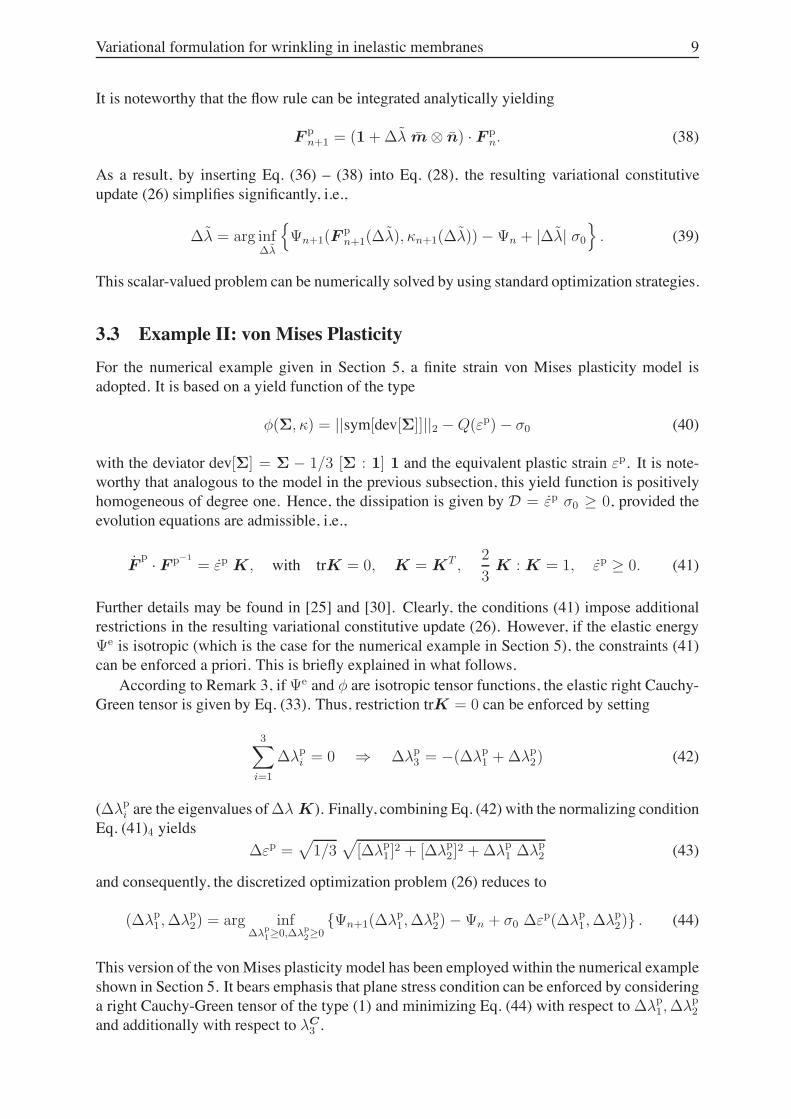
3.3 Example II: von Mises PlasticityFor the numerical example given in Section 5, a finite strain von Mises plasticity model isadopted. It is based on a yield function of the type

&(!, () = ||sym[dev[!]]||2 ) Q()p) ) %0 (40)

with the deviator dev[!] = ! ) 1/3 [! : 1] 1 and the equivalent plastic strain )p. It is note-worthy that analogous to the model in the previous subsection, this yield function is positivelyhomogeneous of degree one. Hence, the dissipation is given by D = )p %0 ( 0, provided theevolution equations are admissible, i.e.,

Fp · F p!1

= )p K, with trK = 0, K = KT ,2

3K : K = 1, )p ( 0. (41)

Further details may be found in [25] and [30]. Clearly, the conditions (41) impose additionalrestrictions in the resulting variational constitutive update (26). However, if the elastic energy"e is isotropic (which is the case for the numerical example in Section 5), the constraints (41)can be enforced a priori. This is briefly explained in what follows.

According to Remark 3, if "e and & are isotropic tensor functions, the elastic right Cauchy-Green tensor is given by Eq. (33). Thus, restriction trK = 0 can be enforced by setting

3/

i=1

##pi = 0 + ##p

3 = )(##p1 +##p

2) (42)

(##pi are the eigenvalues of## K). Finally, combining Eq. (42) with the normalizing condition

Eq. (41)4 yields#)p =

4

1/34

[##p1 ]

2 + [##p2]

2 +##p1 ##p

2 (43)

and consequently, the discretized optimization problem (26) reduces to

(##p1 ,##p

2) = arg inf"#

p1%0,"#

p2%0

{"n+1(##p1,##p

2) )"n + %0 #)p(##p1,##p

2)} . (44)

This version of the vonMises plasticity model has been employed within the numerical exampleshown in Section 5. It bears emphasis that plane stress condition can be enforced by consideringa right Cauchy-Green tensor of the type (1) and minimizing Eq. (44) with respect to ##p

1,##p2

and additionally with respect to #C3 .


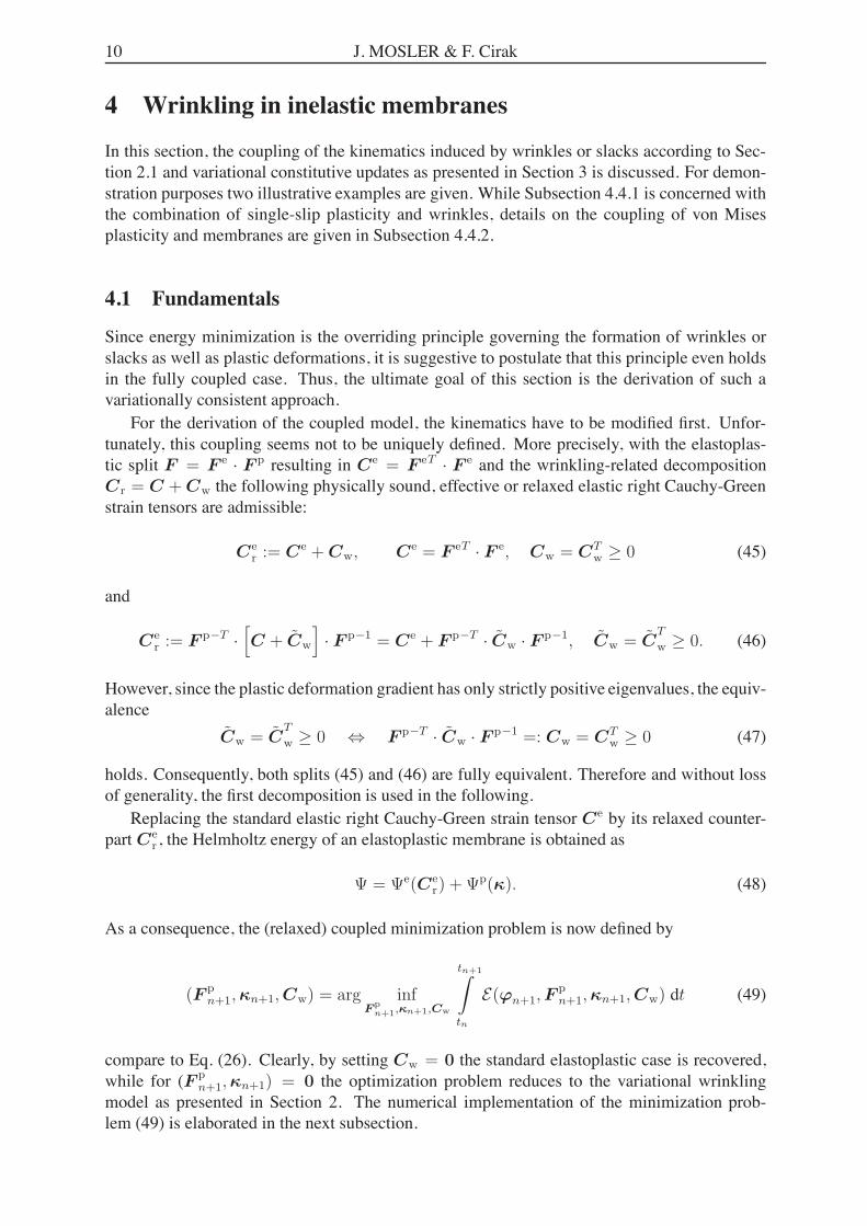
4 Wrinkling in inelastic membranes

In this section, the coupling of the kinematics induced by wrinkles or slacks according to Sec-tion 2.1 and variational constitutive updates as presented in Section 3 is discussed. For demon-stration purposes two illustrative examples are given. While Subsection 4.4.1 is concerned withthe combination of single-slip plasticity and wrinkles, details on the coupling of von Misesplasticity and membranes are given in Subsection 4.4.2.

4.1 Fundamentals

Since energy minimization is the overriding principle governing the formation of wrinkles orslacks as well as plastic deformations, it is suggestive to postulate that this principle even holdsin the fully coupled case. Thus, the ultimate goal of this section is the derivation of such avariationally consistent approach.

For the derivation of the coupled model, the kinematics have to be modified first. Unfor-tunately, this coupling seems not to be uniquely defined. More precisely, with the elastoplas-tic split F = F e · F p resulting in Ce = F eT · F e and the wrinkling-related decompositionCr = C + Cw the following physically sound, effective or relaxed elastic right Cauchy-Greenstrain tensors are admissible:

Cer := Ce + Cw, Ce = F eT · F e, Cw = CT

w ( 0 (45)

and

Cer := F p!T ·

5

C + Cw

6

· F p!1 = Ce + F p!T · Cw · F p!1, Cw = CT

w ( 0. (46)

However, since the plastic deformation gradient has only strictly positive eigenvalues, the equiv-alence

Cw = CT

w ( 0 2 F p!T · Cw · F p!1 =: Cw = CTw ( 0 (47)

holds. Consequently, both splits (45) and (46) are fully equivalent. Therefore and without lossof generality, the first decomposition is used in the following.

Replacing the standard elastic right Cauchy-Green strain tensor Ce by its relaxed counter-part Ce

r , the Helmholtz energy of an elastoplastic membrane is obtained as

" = "e(Cer) +"p(#). (48)

As a consequence, the (relaxed) coupled minimization problem is now defined by

(F pn+1, #n+1, Cw) = arg inf

Fpn+1,"n+1,Cw

tn+1!

tn

E(!n+1, Fpn+1, #n+1, Cw) dt (49)

compare to Eq. (26). Clearly, by setting Cw = 0 the standard elastoplastic case is recovered,while for (F p

n+1, #n+1) = 0 the optimization problem reduces to the variational wrinklingmodel as presented in Section 2. The numerical implementation of the minimization prob-lem (49) is elaborated in the next subsection.


4.2 Numerical implementationFor the numerical implementation, it is convenient to replace the optimization problem (49) bythe equivalent problem

(F pn+1, #n+1, a, b, $, #C

3 ) = arg infF

pn+1,"n+1,a,b,!,#C

3

tn+1!

tn

E dt (50)

cf. Eq. (4). Here, it has been assumed that the considered constitutive model is fully three-dimensional and plane stress conditions are variationally enforced. If the model already fulfillsplane stress conditions, the optimization problem (50) does not depend on the out-of-planestrain component #C

3 . In what follows, attention is restricted to positively homogeneous yieldfunctions of degree one. Hence, the dissipation reads D = # %0 ( 0 (if the stresses andevolution equations are admissible) and thus

tn+1!

tn

E dt = "|tn+1(F p

n+1, #n+1, a, b, $, #C3 ) )"|tn +##(F p

n+1, #n+1) %0. (51)

Clearly, a variation of. tn+1

tnE dtwith respect to the wrinkling parameters (a, b, $) and #C

3 yieldsthe stationarity conditions (14) with the sole exception that the second Piola-Kirchhoff stressesS = 2 "Cr

" are replaced by their counterparts S := 2 "Cer". As a consequence, the variational

problem (51) indeed enforces plane stress conditions and wrinkling is characterized by a one-dimensional stress state. In case of slacks, the stresses vanish completely. Furthermore, since

"Cer

"Ce = Isym (52)

the stationarity conditions corresponding to a variation of. tn+1

tnE dt with respect to the plastic

variables F p and # have the same physical interpretations as those of the standard model (with-out wrinkles or slacks) as explained in Section 3. As a result, wrinkles and slacks in inelasticmembranes (more precisely, in standard dissipative solids) are, as a matter of fact, governed byenergy minimization, cf. Eq. (50).

In principle, minimization problem (50) could be solved by using standard optimizationalgorithms. However, that would be numerically relatively expensive. Furthermore, the problemis not C1-smooth with respect to the plastic variables. For that reason, a coupled predictor-corrector method is applied, cf. [29, 31]. Denoting the trial state of (•) as (•)tr, the elastic,relaxed trial strains are defined as

[Cer]

tr := F pn!T · Cn+1 · F p

n!1. (53)

Accordingly, the trial state is characterized by a purely elastic response (F pn+1 = F p

n) withoutwrinkles or slacks (a = 0, b = 0).

4.2.1 Formation of slacks

Based on the elastic trial strains [Cer ]

tr the largest non-trivial eigenvalue of the tensor [Cer ]

tr )[Ce

r ]tr33 N 3 & N 3 is computed. Let this eigenvalue be denoted as #1. Then, the condition

associated with the formation of slacks reads:

if #1 < 1, a slack forms and Cer = 1, S = 0, F p

n+1 = F pn, #n+1 = #n. (54)

Since the arguments leading to Condition (54) are identical to those for hyperelastic solids,further details are omitted. They may be found in [15].


4.2.2 Standard elastic response without wrinkles or slacks

If Condition (54) is not fulfilled, the formation of wrinkles is checked subsequently. For thatpurpose, the standard solution (no additional plastic deformations and no wrinkles or slacks) isrequired. It is computed from the local minimization problem

#C3 = arg inf

#C3

"n+1(#C3 ) (55)

with a = 0, b = 0 and F pn+1 = F p

n, #n+1 = #n. Finally, the stresses follow from

S = 2 "Cer", with " = inf

#C3

"n+1(#C3 ). (56)

As shown before, the resulting stress state is plane. In the following, the two non-trivial eigen-values of S are denoted as S1 and S2 with S1 > S2.

4.2.3 Wrinkling without additional plastic deformation

It is important to note that due to the interplay between plastic effects and the formation ofwrinkles one cannot estimate if wrinkling occurs by using only the standard solution accordingto Subsection 4.2.2. Consequently, a second predictor-corrector step is applied. More precisely,it is assumed that the considered loading step is purely elastic (F p

n+1 = F pn, #n+1 = #n). In

this case, the wrinkling condition simplifies to

if S2 < 0, wrinkling occurs (57)

cf. [15]. If Condition (57) is fulfilled, the solution associated with the corrector step is obtainedfrom

(a, $, #C3 ) = arg inf

a,!,#C3

"n+1(a, $, #C3 ) (58)

and the stresses are again given by Eq. (56) where " is the reduced minimization problemresulting from Eq. (58).

4.2.4 Plastic deformations without wrinkles or slacks

Based on the predictor steps according to Subsections 4.2.2 or 4.2.3 the discrete loading condi-tion is checked, i.e,

&tr = &(!n+1, Q(#n)) > 0. (59)

If this inequality is not fulfilled, the predictor already represents the physical solution. Oth-erwise a plastic corrector is required. In case of a predictor without wrinkles, the corrector isdefined by the local optimization problem (26). Clearly, the transversal strain component #C

3

has to be included in the minimization problem to guarantee plane stress conditions. It is note-worthy that although the predictor step does not show wrinkles, the converged corrector mayfulfill condition (57). In this case an additional corrector as described in the next subsection isnecessary.

4.2.5 Plastic deformations combined with wrinkling

If the plastic corrector as presented in Subsection 4.2.4 corresponds to wrinkling (Ineq. (57)), orif the wrinkled state according to Subsection 4.2.3 is associated with plastic loading (Ineq. (59)),the fully coupled minimization problem (50) has to be solved numerically (with b = 0).


4.2.6 Resulting algorithm

The resulting algorithm is summarized in Fig. 1 As mentioned before, due to the interplay be-

Initialization: Fpn+1 = F

pn, #n+1 = #n , C

er = [C e

r ]tr

Compute largest eigenvalue !1 of Cer

.

..

....................................................................................................................................................................... .

................................

................................

................................

.................................

................................

................................

.................................

................................

................................

.................................

................................

................................

.................................

................................

.................................

................................

................................

.................................

................................

................................

.................................

................................

................................

.................................

................................

................................

.................................

................................

................................

.................................

................................

................................

.................................

................................

.................................

................................

................................

.................................

................................

................................

.................................

................................

................................

...............

Check slacks; !1 < 1

True False

Cer = 1 Compute smallest eigenvalue S2 of S

.

...............

.................

................

.................

................

.................

................

.................

................

.................

.................

................

.................

................

.................

................

.................

................

.................

................

.................

................

.................

.................

................

.................

................

.................

................

.................

................

.................

................

.................

................

.................

................

.................

.................

................

.................

................

.................

.........

..............................................................................................................................................................................................................................................................................................................................................................................................................................................................................................................................................................................................................................................................................................................................................

Check wrinkling; Eq. (57)

True False

Wrinkling algorithm + Cer

.

....................................................................................................................................................................................................................................................................................................................................................................................... .

.......................................................................................................................................................................................................................................................................................................................................................................................

Check plasticity; Eq. (59)

True False

Coupled algorithm+ C

er , F

pn+1, #n+1

!

Standard elasticity

.

........................................................................................................................................................................................................................................................................................................................................................................................................................................................................................................................................................................................................................... .

..

................................................................................................................................................

Check plasticity; Eq. (59)

True False

Plasticity algorithm+ C

er , F

pn+1, #n+1

.

.....................................................................................................................................................................................................................................................................................................................................................................................................

.

......................................................................................................................................................................................................................................................

Check wrinkling;Eq. (57)True False

Coupled algorithm+ C

er , F

pn+1, #n+1

!

!

!

!

Figure 1: Flow chart of the variationally consistent algorithm for wrinkling in inelastic mem-branes

tween wrinkling and plastic deformation, the predictor (53) is not sufficient to estimate whetherthe resulting state is characterized by plasticity, wrinkling or by both phenomena. Therefore,one additional wrinkling check is required.

4.3 Numerical implementation for fully isotropic models

If "e as well as & are isotropic tensor functions, the numerical implementation can be signifi-cantly simplified. Clearly, the solution associated with the standard case (no plasticity and nowrinkles or slacks) or that corresponding to the formation of slacks can be obtained straight-forward. On the other hand, if only wrinkling occurs (no additional plastic deformation), thewrinkling direction is known in advance, cf. Remarks 2. More precisely, only a scalar-valuedminimization depending on the parameter a has to be solved. In case of plasticity, coaxialitybetween the predictor step and the converged solution can be used, cf. Remark 3, i.e., a return-mapping in principal axes, refer to [29]. As a consequence, the only remaining case is the fullycoupled one (wrinkling combined with plastic effects).

However, it can be shown in a relatively straightforward manner that even in the coupledcase, the relaxed elastic right Cauchy-Green tensor Ce

r is coaxial to its trial counterpart. Moreprecisely, with the spectral decomposition of the elastic trial strains

[Cer ]

tr =3

/

i=1

0

#Cetrr

i

12

N i & N i (60)


and enforcing #Cer

1 > #Cer

2 = #Cer

3 which follows from isotropy of "e together with the uniaxialstress state characterizing wrinkling, the wrinkling related tensor Cw shows the form

Cw = a2 N 2 & N 2. (61)

Here, N 2 represents the wrinkling direction and N 3 denotes the normal of the membrane. Asa result, the spectral decomposition of Ce

r can be written as

[Cer ]n+1 :=

0

#Cetrr

1

12

exp[)2 ##p1 ] N 1 & N 1

+

70

#Cetrr

2

12

exp[)2 ##p2] + a2

8

[1 ) N 1 & N 1].(62)

Again,##pi are the eigenvalues of ## K, i.e.,

## K =3/

i=1

##pi N i & N i (63)

cf. Remark. 3. As a result, the minimization problem (50) with b = 0 reduces to

(##p1 ,##p

2, a) = arg inf"#

p1 ,"#

p2 ,a

{"n+1(##p1 ,##p

2, a) )"n + %0 ##(##p1 ,##p

2)} . (64)

Here, isotropic hardening of the type (n+1 = (n + f(##p1,##p

2) has been assumed.Clearly, different solution schemes can be used to solve the minimization problem (64). In

the present paper, a limited memory BFGS method [32] is applied. It requires the gradient ofthe function

"(##p1,##p

2, a) := {"n+1(##p1 ,##p

2, a) )"n + %0 ##(##p1 ,##p

2)} (65)

to be minimized. After a straightforward calculation it results in

""

"a= a [S2 + S3] (66)

""

"##p1

= )0

#Cetrr

1

12

exp[)2 ##p1 ] S1 +

""p

"(

"(

"##p1

(67)

""

"##p1

= )0

#Cetrr

2

12

exp[)2 ##p2] [S2 + S3] +

""p

"(

"(

"##p2

. (68)

Again, Si = S : (N i & N i) are the eigenvalues of the second Piola-Kirchhoff-type tensorS = 2 "Ce

r"e. If Newton’s method is to be applied, the second derivatives are necessary, too.

They can be simply obtained by using

"Si

"a= a (N i & N i) : C : (1 ) N 1 & N 1) , C = 4 "Ce

rCer"e (69)

"Si

"##p1

= )0

#Cetrr

1

12

exp[)2 ##p1 ] (N i & N i) : C : (N 1 & N 1) (70)

"Si

"##p2

= )0

#Cetrr

2

12

exp[)2 ##p1] (N i & N i) : C : (1 ) N 1 & N 1). (71)

Obviously, for a quadratic convergence at structural level, the linearization of " with respectto the total strains F is required. However, it can be derived in standard manner. Therefore,further details are omitted.


0 0.2 0.4 0.6 0.8 10

0.5

1

1.5

2

2.5

3

(a)

!! = |!!|

Energy

"n+

1

0.10.080.060.040.020

5510

5460

5410

5360

(b)

Figure 2: Single slip plasticity; energy landscape of the incremental potential. tn+1

tnE dt: (a) no

plastic deformations; the potential depends only on the wrinkling parameters a (horizontal) and$ (vertical), (b) no wrinkling

4.4 Illustrative examplesFor the sake of comprehensibility, two prototype models are presented in this subsection. Whilesingle slip plasticity theory is briefly addressed in Subsection 4.4.1, Subsection 4.4.2 is con-cerned with a von Mises type plasticity model. In both cases, the elastic response is governedby a neo-Hooke type model with Lame constants # = 117818 N/mm2 and µ = 81000 N/mm2.The yield limit is chosen identically as well (%0 = 360 N/mm2).

4.4.1 Example I: single slip system

If single slip plasticity theory is included in a membrane formulation, special attention is re-quired to avoid inadmissible transverse shear strains. For that purpose, it is assumed that theslip system belongs to the tangent space of the membrane (with respect to the intermediateconfiguration). More precisely, m = E1 and n = E2 with Ei denoting the standard cartesianbases, see Subsection 3.2. Hence, the out-of-plane response inE3 direction is purely elastic. Onthis account, it is convenient to enforce plane stress condition a priori. This can be achieved bydirectly starting with a reduced elastic strain energy"e, cf. the Appendix in [15]. Consequently,"e used in the present Subsection 4.4.1 does not depend on #C

3 anymore.As mentioned before, in case of slacks, the local optimization problem (50) has a trivial

solution, cf. Eq. (54). Thus, it is sufficient to consider the minimization problem

(##, a, $) = arg inf"#,a,!

2

"n+1(##, a, $) )"n + %0 |##|3

(72)

see Subsection 3.2. In a first step, the fully uncoupled cases are analyzed. While in Fig. 2(a)plastic effects are neglected, wrinkling is excluded in Fig. 2(b). Both figures are based on thesame incremental potential. More precisely, a (two-dimensional) deformation gradient of thetype

F = 1 +1

2* (E1 + E2) & (E1 ) E2) + ) E1 & E1 (73)


"

!

a

Figure 3: Single slip plasticity; energy landscape of the incremental potential. tn+1

tnE dt for the

fully coupled case (wrinkling combined with plastic deformations)

with * = 0.5 and ) = )0.2 is assumed (again, Ei are the standard cartesian bases). It cor-respond to a simple shear deformation superposed by a compression in E1 direction. For theelastic response, a two-dimensional neo-Hooke model is adopted, cf. the Appendix in [15].Hardening effects are neglected, i.e., "p = 0. According to Fig. 2, plasticity as well as wrin-kling relax the physical problem, i.e., they result in an energy decrease. While wrinkling showsa significant impact on the energy (87% reduction in energy compared to the standard fully elas-tic case), plastic effects are comparably small (4% reduction in energy compared to the standardfully elastic case).

Next, the fully coupled problem is investigated. Clearly, the resulting energy has to be lowerthan (or equal to) that associated with uncoupled wrinkling. The computed energy landscapedepending on the plastic slip ## and the wrinkling parameters a and $ is shown in Fig. 3.It bears emphasis that the yield function is not isotropic and hence, coaxiality between theelastic trial strains and the converged relaxed elastic strains is not fulfilled. As a result, theminimization problem (72) cannot be further simplified. Indeed, at the minimum as illustratedin Fig. 3 the wrinkling direction does not coincide with one of the eigenvectors of the elastictrial strains. The relaxed problem leads to a reduction in energy of about 88% compared to thestandard, fully elastic solution. For the sake of comparison, the energies as predicted by thedifferent schemes are summarized in Tab. 1.

4.4.2 Example II: von Mises Plasticity

In contrast to single slip plasticity theory, the proposed von Mises type model is purely isotropic("e as well as &). Consequently, the algorithm as presented in Subsection 4.3 can be employedwith the sole exception that the strain-like internal variable ( is replaced by the equivalent


Model Energy [%] Reduction in energy [%]Standard 100 /Plasticity 96 4Wrinkling 13 87Coupled 12 88

Table 1: Single slip plasticity; energies resulting from different models.

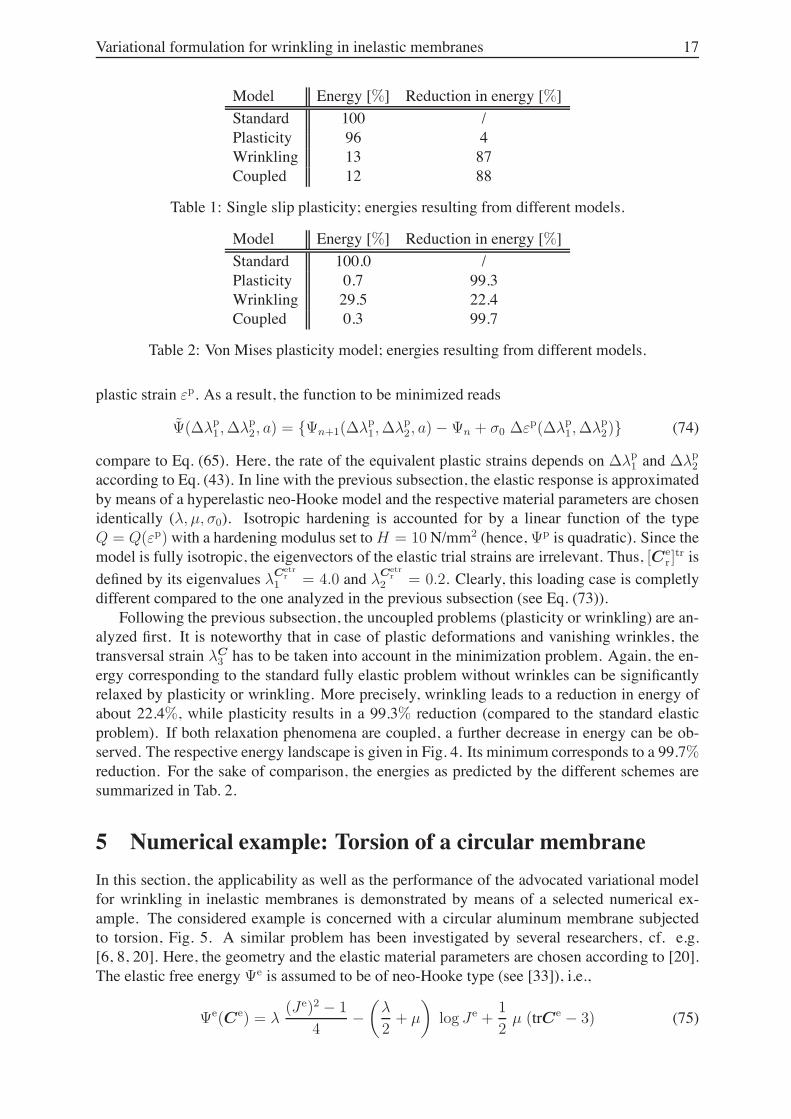
Model Energy [%] Reduction in energy [%]Standard 100.0 /Plasticity 0.7 99.3Wrinkling 29.5 22.4Coupled 0.3 99.7

Table 2: Von Mises plasticity model; energies resulting from different models.

plastic strain )p. As a result, the function to be minimized reads

"(##p1 ,##p

2, a) = {"n+1(##p1,##p

2, a) )"n + %0 #)p(##p1,##p

2)} (74)

compare to Eq. (65). Here, the rate of the equivalent plastic strains depends on ##p1 and ##p

2

according to Eq. (43). In line with the previous subsection, the elastic response is approximatedby means of a hyperelastic neo-Hooke model and the respective material parameters are chosenidentically (#, µ, %0). Isotropic hardening is accounted for by a linear function of the typeQ = Q()p) with a hardening modulus set toH = 10N/mm2 (hence, "p is quadratic). Since themodel is fully isotropic, the eigenvectors of the elastic trial strains are irrelevant. Thus, [Ce

r ]tr is

defined by its eigenvalues #Cetrr

1 = 4.0 and #Cetrr

2 = 0.2. Clearly, this loading case is completlydifferent compared to the one analyzed in the previous subsection (see Eq. (73)).

Following the previous subsection, the uncoupled problems (plasticity or wrinkling) are an-alyzed first. It is noteworthy that in case of plastic deformations and vanishing wrinkles, thetransversal strain #C

3 has to be taken into account in the minimization problem. Again, the en-ergy corresponding to the standard fully elastic problem without wrinkles can be significantlyrelaxed by plasticity or wrinkling. More precisely, wrinkling leads to a reduction in energy ofabout 22.4%, while plasticity results in a 99.3% reduction (compared to the standard elasticproblem). If both relaxation phenomena are coupled, a further decrease in energy can be ob-served. The respective energy landscape is given in Fig. 4. Its minimum corresponds to a 99.7%reduction. For the sake of comparison, the energies as predicted by the different schemes aresummarized in Tab. 2.

5 Numerical example: Torsion of a circular membraneIn this section, the applicability as well as the performance of the advocated variational modelfor wrinkling in inelastic membranes is demonstrated by means of a selected numerical ex-ample. The considered example is concerned with a circular aluminum membrane subjectedto torsion, Fig. 5. A similar problem has been investigated by several researchers, cf. e.g.[6, 8, 20]. Here, the geometry and the elastic material parameters are chosen according to [20].The elastic free energy "e is assumed to be of neo-Hooke type (see [33]), i.e.,

"e(Ce) = #(Je)2 ) 1

4)

9#

2+ µ

:

log Je +1

2µ (trCe ) 3) (75)


!p2

a

!p1

Figure 4: Von Mises plasticity; energy landscape of the incremental potential " for the fullycoupled case (wrinkling combined with plastic deformations)

withJe =

3det Ce, trCe = Ce : 1. (76)

The membrane having a thickness of t = 0.01mm is clamped at the outer as well as at theinner boundary and loading is applied by increasing the angle + at the inner boundary up to+max = 1.8$ = 0.03176rad. Subsequently, the angle + is decreased up to + = 0rad. In contrastto introduced illustrative examples, the problem has been experimentally analyzed as well, cf.[20]. Due to the relatively large strains, plastic effects can be observed in the experiment.Hence, a plasticity model is needed to guarantee a realistic finite element approximation. Here,the von Mises model as summarized in Subsection 3.3 is adopted. Isotropic hardening is takeninto account by a potential of the type, "()p) = 1/2 H()p)2, with H being the (constant)hardening modulus. The material parameters characterizing an aluminum membrane are givenin Fig. 5.

Based on the introduced, fully variational algorithmic formulation for inelastic membranesa finite element analysis of the circular membrane has been performed. The underlying spatialdiscretization is depicted in Fig. 5. It contains 1072 bi-quadratic 6 node triangular elements.Both the local wrinkling-related minimization problems according to Subsection 4.2 or 4.3 aswell as the resulting global optimization problem (15) are solved by using the limited memoryBFGS method [32].

The predicted reaction momentum vs. angle diagram is shown in Fig. 6. For the sake ofcomparison, the numerical results reported in [20], together with the experimentally observedstructural behavior (cf. [20]), are also included. During the first loading stage (+ is increasedfrom 0 up to +max = 1.8$ = 0.03176rad) the good agreement between the experiment and thenovel algorithmic formulation is noteworthy. In contrast to the model by Hornig & Schoopthe ultimate load (momentum) is not overestimated. However, although the novel results are


rari

#

Material parametersElastic model; Eq. (75) Plastic model; Subsection 3.3# 40384.6 N/mm2 %0 130.0 N/mm2

µ 26923.1 N/mm2 H 500.0 N/mm2

"p 1/2H ()p)2 (linear hardening)

Figure 5: Torsion of an elastoplastic circular membrane: boundary conditions and materialparameters. The membrane is clamped at both radii. The dimensions are ra = 125 mm, ri =45 mm; the thickness is t = 0.01 mm.

Experiment; Hornig et al.FEM; Hornig et al.FEM; novel method

Angle # [rad]

Reactionmomentum[Nmm]

0.030.020.010

20000

10000

0

-10000

-20000

Figure 6: Torsion of an elastoplastic circular membrane: momentum vs. angle diagram


Wrinkling amplitudes anddirections

Plastic strains )p

Results at point!;see Fig. 6

Results at point4;see Fig. 6

Figure 7: Torsion of a circular membrane: distribution of the wrinkling strains and equivalentplastic strains )p. The plots on the left hand side are associated with +max = 0.03176rad (point! in Fig. 6), while the plots on the right hand side correspond to the point4 in Fig. 6.

significantly more realistic than those shown in [20] even during the second loading stage (+is decreased from +max = 1.8$ = 0.03176rad up to 0), a slight difference compared to theexperimentally determined curve is obvious. A careful analysis of the diagram reveals threepossible explanations: (1) The experimental data seems to scatter; (2) The initially flat mem-brane is transformed into a corrugated plate during the loading stage which changes the struc-tural stiffness of the membrane for the subsequent unloading and load reversal stage; (3) Duringunloading (+ decreases and varies between 0.025rad and 0.015rad) the structure is not fully un-loaded (non-vanishing momentum). Hence, kinematic hardening which is not included withinthe numerical model plays a non-negligible role. It bears emphasis that although only isotropichardening is taken into account within the variational algorithm, the modifications necessaryfor the kinematic counterpart are straightforward, cf. [25–27].

The wrinkling directions and amplitudes, together with the plots of the equivalent plasticstrain )p are summarized in Fig.7. The plots on the right hand side are associated with +max =0.03176rad. It can be seen that, as expected, the wrinkles point into the loading direction.Furthermore, the inelastic strains are localized at the inner boundary. If the angle + is decreased,the amplitudes of the wrinkles also decrease first. However, at a certain stage and in contrastto the fully elastic problem, wrinkling in the current loading direction occurs. Furthermore,additional inelastic deformations can be observed. The wrinkling pattern is in good agreement


with that reported in [20].Interestingly, numerical problems have arisen in [20] during the computations. They have

been reduced by deriving an initial guess for the employed Newton’s scheme. It is noteworthythat such numerical problems have not been observed in the presented finite element formu-lation. Furthermore, even if numerical instabilities become dominant in the novel variationalapproach, a (standard) more sophisticated optimization method can be adopted without anyadditional effort, cf. [34].

6 ConclusionIn this paper, a novel, fully variational formulation suitable for wrinkling in inelastic membranesat finite strains was presented. The distinguishing character of the new approach is that everyaspect of the considered physical problem is driven by energy minimization. An introductionof ad-hoc loading conditions is not required, but they follow naturally from the mathematicallyand physically sound variational principle itself. Based on relaxing an incrementally definedenergy functional, the plastic strains, the internal variables, together with the wrinkling pat-terns, are jointly computed. Furthermore, by doing so, a reduced functional depending only onthe standard strains is derived which acts like a hyperelastic potential for the stresses. Moreprecisely, the stresses result from differentiating this potential with respect to the strains. Con-sequently, the method is formally identical to standard hyperelasticity with the sole exceptionthat the aforementioned potential is locally defined (in time).

In line with the theoretical part of the present paper, the proposed numerical implementa-tion is based on the same variational structure, i.e., after applying a time discretization to theevolution equations, all unknown variables are computed by employing classical minimizationalgorithms. As a result, the numerical formulation is relatively straightforward and the result-ing algorithm inherits the efficiency and robustness properties of the underlying optimizationscheme. In particular for highly non-linear problems such as wrinkling in membranes thisrepresents an important advantage of the advocated idea compared to previous approaches. Itbears emphasis that the presented implementation does not rely on any symmetry assumptionsconcerning the elastic response or the yield function. For fully isotropic models, an adaptednumerical implementation in principal stress space was derived.

In the present paper, only dissipative effects resulting from rate-independent plasticity havebeen considered. However, since many rate effects can also be described in a variationallyconsistent manner, cf. [25, 35], their incorporation into the novel variational membrane modelis relatively straightforward. The same holds true for the fully thermo-mechanically coupledproblem, cf. [36].

References[1] H. Wagner. Ebene Blechwandtrager mit sehr dunnen Stegblechen. Z. Flugtechnik u.

Motorluftschiffahrt, 20, 1929.

[2] E Reissner. On tension field theory. In Fifth Int. Cong. on Appl. Mech., pages 88–92,1938.

[3] D.G. Roddeman, J. Drukker, C.W.J. Oomens, and J.D. Janssen. The wrinkling of thinmembranes: Part I – theory. Journal of Applied Mechanics, 54:884–887, 1987.


[4] D.G. Roddeman, J. Drukker, C.W.J. Oomens, and J.D. Janssen. The wrinkling of thinmembranes: Part I – numerical analysis. Journal of Applied Mechanics, 54:888–892,1987.

[5] H. Schoop, L. Taenzer, and J. Hornig. Wrinkling of nonlinear membranes. ComputationalMechanics, 29:68–74, 2002.

[6] R. Rossi, M. Lazzari, R. Vitaliani, and E. Onate. Simulation of light-weight membranestructures by wrinkling model. International Journal for Numerical Methods in Engineer-ing, 62:2127–2153, 2005.

[7] T. Raible, K. Tegeler, S. Lohnert, and P. Wriggers. Development of a wrinkling algo-rithm for orthotropic membrane materials. Computer Methods in Applied Mechanics andEngineering, 194:2550–2568, 2005.

[8] M. Miyazaki. Wrinkle/slack model and finite element dynamics of membranes. Interna-tional Journal for Numerical Methods in Engineering, 66:1179–1209, 2006.

[9] A. Jarasjarungkiat, R. Wuechner, and K.U. Bletzinger. A wrinkling model based on mate-rial modification for isotropic and orthotropic membranes. Computer Methods in AppliedMechanics and Engineering, 197:773–788, 2008.

[10] D.J. Steigmann. Tension-Field theory. Proceedings of the Royal Society of London. SeriesA, Mathematical and Physical Science, 429:141–173, 1990.

[11] A.C. Pipkin. The relaxed energy density for isotropic elastic membranes. IMA Journal ofApplied Mathematics, 36:85–99, 1986.

[12] A.C. Pipkin. Convexity conditions for strain-dependent energy functions for membranes.Arch. Rational Mech. Anal., 121:361–376, 1993.

[13] A.C. Pipkin. Relaxed energy densities for large deformations of membranes. IMA Journalof Applied Mathematics, 52:297–308, 1994.

[14] M. Epstein. On the wrinkling of anisotropic membranes. Journal of Elasticity, 55:99–109,1999.

[15] J. Mosler. A novel variational algorithmic formulation for wrinkling at finite strains basedon energy minimization: application to mesh adaption. Computer Methods in AppliedMechanics and Engineering, 197:1131–1146, 2008.

[16] Arthur Lyons. Materials for Architects & Builders. Butterworth-Heinemann, 3rd edition,2006.

[17] Xi Wang and Jian Cao. On the prediction of side-wall wrinkling in sheet metal formingprocesses. International Journal of Mechanical Sciences, 42:2369–2394, 2000.

[18] Eran Sharon, Benoit Roman, and Harry L. Swinney. Geometrically driven wrinkling ob-served in free plastic sheets and leaves. Physical Review E, 75(4), 2007.

[19] J. Hornig. Analyse der Faltenbildung in Membranen aus unterschiedlichen Materialien.PhD thesis, Technische Universitat Berlin, 2004.

[20] J. Hornig and H. Schoop. Wrinkling analysis of membranes with elastic-plastic materialbehavior. Computational Mechanics, 35:153–160, 2005.


[21] J. Mosler and M. Ortiz. On the numerical implementation of variational arbitraryLagrangian-Eulerian (VALE) formulations. International Journal for Numerical Meth-ods in Engineering, 67:1272–1289, 2006.

[22] J. Mosler. On the numerical modeling of localized material failure at finite strains bymeans of variational mesh adaption and cohesive elements. Habilitation, Ruhr UniversityBochum, Germany, 2007.

[23] J. Mosler and M. Ortiz. Variational h-adaption in finite deformation elasticity and plastic-ity. International Journal for Numerical Methods in Engineering, 72:505–523, 2007.

[24] F. Cirak and M. Ortiz. Fully c1-conforming subdivision elements for finite deformationthin-shell analysis. International Journal for Numerical Methods in Engineering, 51:813–833, 2001.

[25] M. Ortiz and L. Stainier. The variational formulation of viscoplastic constitutive updates.Computer Methods in Applied Mechanics and Engineering, 171:419–444, 1999.

[26] C. Carstensen, K. Hackl, and A. Mielke. Non-convex potentials and microstructures infinite-strain plasticity. Proc. R. Soc. Lond. A, 458:299–317, 2002.

[27] M. Ortiz. Computational Solid Mechanics – Lecture Notes. California Institute of Tech-nology, 2002.

[28] B. Halphen and Q.S. Nguyen. Sur les materiaux standards generalises. J. Mechanique,14:39–63, 1975.

[29] J.C. Simo. Numerical analysis and simulation of plasticity. In P.G. Ciarlet and J.J. Lions,editors, Handbook for numerical analysis, volume IV. Elsevier, Amsterdam, 1998.

[30] J. Alberty, C. Carstensen, and D. Zarrabi. Adaptive numerical analysis in primal elasto-plasticity with hardening. Computer Methods in Applied Mechanics and Engineering,171:175–204, 1999.

[31] J.C. Simo and T.J.R. Hughes. Computational inelasticity. Springer, New York, 1998.

[32] D.C. Liu and J. Nocedal. On the limited memory method for large scale optimization.Mathematical Programming B, 45(3):503–528, 1989.

[33] P. Ciarlet. Mathematical elasticity. Volume I: Three-dimensional elasticity. North-HollandPublishing Company, Amsterdam, 1988.

[34] C. Geiger and C. Kanzow. Numerische Verfahren zur Losung unrestringierter Opti-mierungsaufgaben. Springer, 1999.

[35] E. Fancello, J.-P. Ponthot, and L. Stainier. A variational formulation of constitutive mod-els and updates in non-linear finite viscoelasticity. International Journal for NumericalMethods in Engineering, 65:1831–1864, 2006.

[36] Q. Yang, L. Stainier, and M. Ortiz. A variational formulation of the coupled thermo-mechanical boundary-value problem for general dissipative solids. Journal of the Me-chanics and Physics of Solids, 54:401–424, 2006.

Documents

A variational form ulation for Þ nite deform ation w … · w rinkling analysis of inelastic m em branes J.M osler M aterials M echanics Institute for M aterials R esearch G K SS