A variable redefinition approach for the lot sizing problem with strong set-up interactions

A variable rede®nition approach for the lot sizing problemwith strong set-up interactions

MANISH BHATIA and UDATTA S. PALEKAR

Department of Mechanical and Industrial Engineering, University of Illinois at Urbana-Champaign, Urbana, IL 61801, USAE-mail: manish [email protected]; [email protected]

Received February 1998 and accepted April 1999

We address a variant of the Joint Replenishment Problem, in which the products can only be produced in ®xed proportions to eachother. Such problems occur commonly in the manufacture of sheet metal and die-cast parts and some chemical products. We call itthe Strong Interaction Problem (SIP). The general instance of the problem is NP-complete while single nest instances are poly-nomially solvable. We establish the boundary at which the problem becomes hard. We also present an exact algorithm for solvingthe problem using a variable rede®nition approach. Computational testing on randomly generated problems indicates that ouralgorithm is several orders of magnitude faster than solution of the problems without reformulation using existing algorithms andcommercial software.

1. Introduction

We address the problem of determining economic lot-sizes when a group of parts are co-manufactured. Ourfocus is on problems in which products belong to variousnests or families, and all parts in a nest are produced in®xed proportion to each other. We call this the StrongInteraction Problem. Such problems occur commonly inthe manufacture of sheet metal and die-cast parts and insome chemical manufacturing problems. In die-castingand sheet metal operations the number and type of partsproduced depends on the die used. Once designed, the diecharacterizes the nest and all parts are produced simul-taneously and in a ®xed proportion, depending on the dieused. Similarly, in the chemical industry the process pa-rameters used de®ne the proportions of the variouschemicals produced, and thus characterize the variousnests.This problem is a variant of the well known Joint

Replenishment Problem (JRP) (Aksoy and Erenguc,1988; Arkin et al., 1989; Stowers, 1993; Federgruen andTzur, 1994; Stowers and Palekar, 1994). The JRP involvesdetermining lot-sizes to satisfy known demands of agroup of parts, in each period of the planning horizon, atminimum cost. An unlimited amount may be produced ineach period of the horizon. The cost structure consists ofjoint set-up costs paid whenever any product is manu-factured, individual set-up cost for each product manu-factured and inventory holding costs proportional to theend of period inventory levels. Arkin et al. (1989) showedthat the JRP is NP-complete. The SIP di�ers from the

JRP in that products belong to more than one nest, andproduction quantities of parts in a nest are constrained tobe proportional.The SIP was ®rst addressed by Stowers and Palekar

(1997). They consider a K period, M product and N nestproblem. Each product belongs to some of the availablenests. The demand for each product is known and is to bemet, without backlogging, using the available nests. Thecost structure consists of the set-up and variable pro-duction costs for the nests, and a holding cost propor-tional to the end of period inventory levels.Stowers and Palekar (1997) showed that the problem is

NP-hard, and remains NP-hard given any set-up se-quence. The single nest instances are, however, polyno-mially solvable. This result is in direct contrast to the JRPwhich is NP-complete. The additional restriction thatproducts must be made in ®xed proportion makes theproblem easier to solve in this case. Instances of the SIPin which each product is present in at least two familiesare shown to be NP-hard. Also, determining if a zero ®nalinventory solution to the SIP exists is NP-complete.Stowers and Palekar (1997) presented various mathe-matical formulations of the problem, and a branch-and-bound-based algorithm to solve it. The bounds arecalculated by solving a Lagrangean relaxation of theproblem, obtained by dropping the proportionalityconstraints.In this paper, we present an alternative algorithm for

solving the above model using the variable rede®nitionapproach discussed by Eppen and Martin (1987) andMartin (1987). We restrict ourselves to the continuous

IIE Transactions (2001) 33, 357±370

0740-817X Ó 2001 ``IIE''

production variant of the problem. This is done for tworeasons. First, in many situations, like chemical process-ing, the production variables are continuous. Second, forlarge demands this is a good approximation of the dis-crete quantity solution (Gilmore and Gomory, 1963).The paper is organized as follows. Section 2 provides

a mathematical formulation of the problem and an al-ternate proof of the complexity of the problem. InSection 3 we develop a reformulation of the problem. InSection 4 we discuss an enumerative approach to solvethe SIP. Section 5 discusses our computational experi-ence with the problem. Finally, we conclude the paper inSection 6.

2. Lot-sizing with strong set-up interactions

The SIP involves determining the set-ups and lot-sizes foreach nest required to satisfy demands for the di�erentproducts. The model speci®es a horizon of a ®nite num-ber of periods, a set of nests and the multiplicity of eachproduct in each nest. The cost structure comprises of theset-up and variable production costs for the nests and theinventory holding cost for the products. The objective isto satisfy the demands, without backlogging, at minimumcost.In this section we present various mathematical for-

mulations of the problem. We also provide an alternateproof that the SIP is NP-complete.

2.1. Mathematical formulations

The following notation is used in the remaining sections.Let

i = index of products, i � 1; . . . ;M ;j = index of nests, j � 1; . . . ;N ;k = index of time periods, k � 1; . . . ;K;

Vjk = variable production cost of family j in periodk;

Hik = holding cost for product i in period k;Sjk = set-up cost for nest j in period k;dik = demand for product i in period k;Dik =

Pkt�1 dit = cumulative demand for product i

through period k;Dikt = Di;tÿ1 ÿ Di;kÿ1 = cumulative demand be-

tween periods k and t ÿ 1;aij = the multiplicity of product i in family j;

Xjk = the number of units of family j produced inperiod k;

Yjk = the set-up variable for family j in period k;Iik =

Pj

Pt�k aijXjt ÿ Dik, inventory of product i

at end of period k;Mjk = suitably large number;Ji = fj : aij > 0g, the set of nests to which product

i belongs;

Ij = fi : aij > 0g, the set of products belonging tonest j.

conv�� = the convex hull of set (�).The problem can mathematically be formulated as fol-lows:

m�P��minX

j

Xk

VjkXjk�X

i

Xk

Hik

Xj

Xt�k

aijXjtÿDik

!

�X

j

Xk

SjkYjk; �1�

subject to Xj

Xt�k

aijXjt � Dik 8 i; k; �2�

Xjk � MjkYjk 8 j; k; �3�Xjk 2 R� 8 j; k; �4�

Yjk 2 f0; 1g 8 j; k: �5�If we let a �Pi

Pk HikDik and Pjk � Vjk �

Pi

Pt�k Hitaij,

the objective function can be simpli®ed to obtain

m�P� � minX

j

Xk

PjkXjk �X

j

Xk

SjkYjk ÿ a: �6�

Also Mjk can be given the value

Mjk � maxfi2Ijg

DiT ÿ Di;kÿ1aij

:

An alternate disaggregated formulation of the problemwas presented by Stowers and Palekar (1997). Let Xijk bethe amount of product i produced using family j in periodk. Let Yijk be the set-up variable for product i using familyj in period k. Also, let

Mijk � aijMjk; Vijk � VjkPi aij

;

Pijk � Vijk �Xt�k

Hit; Sijk � Sjk

jIjj :

Then the following is an alternate disaggregated formu-lation of the SIP.

m�WP� � minX

i

Xj

Xk

PijkXijk �X

i

Xj

Xk

SijkYijk ÿ a;

�7�subject to

ai1jXi2jk � ai2jXi1jk 8 i1; i2 2 Ij; j; k; �8�Yi1jk � Yi2jk 8 i1; i2 2 Ij; j; k; �9�X

j

Xt�k

Xijt � Dik 8 i; k; �10�

Xijk � MijkYijk 8 i; j; k; �11�Xijk 2 R� 8 i; j; k; �12�

358 Bhatia and Palekar

Yijk 2 f0; 1g 8 i; j; k: �13�Stowers and Palekar (1997) solved the above continu-

ous production variant of the SIP using a branch-and-bound approach. The bounds were obtained by solvingproblem WPl, the Lagrangean relaxation of WP withrespect to constraints (8). We also restrict ourselves to thecontinuous production variant. In addition, we make thestandard assumption that there is no initial inventory.

2.2. Complexity issues

Stowers and Palekar (1997) provided a transformationfrom the NP-complete vertex cover problem to show thatthe SIP is NP-complete. They also provided a transfor-mation from the NP-complete minimum cover problemto show that the SIP remains NP-complete given any set-up sequence. Their proof relies on the complexity createdby the structure of the nests. A polynomial time algo-rithm to ®nd the optimal production sequence given a set-up sequence was provided for instances of the SIP withonly two nests. We provide an alternate proof to showthat the SIP remains NP-complete even for simple neststructures.

Proposition 1. Given any instance of the SIP with twonests and two products only one of which is present in bothnests and where parts occur with multiplicity zero or one,determining whether there exists a solution to the SIP withvalue less than U is NP-complete.

Proof. Obviously any solution can be veri®ed in poly-nomial time, hence we know the problem is in class NP.We now construct a transformation from the known NP-complete Capacitated Lot-Sizing Problem (CLSP) to thisinstance of the SIP.(CLSP) instance.Given a number K 2 Z� and K > 0 of

periods, for each period k, 1 � k � K, a demand rk 2 Z�,a production capacity ck 2 Z�, a production set-up costbk 2 Z�, an incremental production cost vk 2 Z�, an in-ventory cost coe�cient �hk 2 Z� and an overall boundU 2 Z�.Question. Do there exist production amounts xk 2 Z�,

associated inventory levels ik �Pj�k

j�1�xj ÿ rj�, and asso-ciated set-up variables wk 2 f0; 1g such that

xk � ck 8 k; ik � 0 8 k;

wk � 1 if xk > 0,0 otherwise,

�and

mCLSP �X

k

�vkxk � �hkik � skwk� � U ?

Given an instance of the CLSP, construct a two nest,two product and K period instance of the SIP as follows.

For clarity we name the nests A and B and the products 1and 2. Let

a1A � 1; a1B � 0; a2A � 1;

a2B � 1; d1k � rk 8 k; d2k � ck 8 k;

SAk � bk 8 k; SBk � 0 8 k; h1k � �hk 8 k;

h2k � 1 8 k; VAk � vk 8 k and VBk � 0 8 k:

Clearly, this transformation can be done in polyno-mial time. Suppose 9 a solution to the SIP withvalue mSIP � U . Since, U is ®nite, I2k � 0 8 k whichyields XAk � XBk � d2k � ck 8 k. Also, since product 1is present only in nest A with a multiplicity of one,I1k �

Pt�k�XAtÿ d1t� � 0 8 k: Construct a solution for

the CLSP, with xk � XAk, ik � I1k and wk � YAk.Clearly, this solution is feasible to the CLSP and has acost of mSIP.Now suppose 9 a solution to the CLSP with value

mCLSP � U . Construct a solution to the SIP as follows.

XAk � xk � ck 8 k; �14�XBk � ck ÿ xk � 0 8 k; �15�

YAk � wk 8 k; �16�YBk � 1 8 k; �17�

Clearly, I1k � ik � 0 8 k, X2k � XAk � XBk � ck � d2k andI2k � 0 8 k. Thus this solution is feasible to the SIP andhas a cost of mCLSP.Hence, the CLSP has a solution of cost less than U i�

the given instance of the SIP has cost less than U . Thus,solving the CLSP is equivalent to solving the SIP. j

Corollary 1. The SIP with only two nests is NP-hard.

Stowers and Palekar (1997) showed that the single nestSIP is polynomially solvable. Proposition 1 and Corollary1 show that the two nest SIP is NP-complete. This es-tablishes the boundary at which the problem becomeshard.

3. Reformulation of SIP

In this section, we discuss a reformulation of the SIPusing the method of variable rede®nition describedby Eppen and Martin (1987) and Martin (1987). Thebasic idea of this approach is to recognize a specialstructure sub-problem, say Q, and develop an alternateformulation, say Z, which is strongly equivalent seeMartin (1987) to Q under a linear transformation T .The following propositions from Martin (1987) willthen hold.

Proposition 2. If Z is equivalent to Q under T, andT ��Z� � �Q, then z, xj; 8 j 2 J optimal in MIP2 impliesx � Tz is optimal to MIP.

Variable rede®nition approach for the lot sizing problem 359

Proposition 3. If conv�Z� � �Z and Z is strongly equivalentto Q under T, then the LP relaxation of MIP2 yieldsbounds equal to solving the Lagrangean dual of problemMIP with respect to constraints Ax � a.

3.1. Multi-source uncapacitated lot-sizing problem

In this section we recognize a special structure sub-problem in model WP and develop an alternative for-mulation, which is, strongly equivalent to formulationWP. Note that if we drop the ``complicating'' constraints(8) and (9) of model WP the problem breaks up intoM Multi-source Uncapacitated Lot-Sizing Problems(MULSP), one for each product. The MULSP is avariant of the Uncapacitated Lot-Sizing Problem(ULSP), in which each product can be manufacturedusing a number of di�erent ``sources'' or techniques,each having a di�erent set-up cost associated with it.The Wagner±Whitin properties for the ULSP also holdfor the MULSP and its complexity is the same asthe ULSP. The MULSP can easily be transformedinto a ULSP with concave costs (Zangwill, 1969).However, for the purpose of reformulation, we need tocharacterize all extreme points of the feasible region of aMULSP.Before we establish some properties of the MULSP,

consider the following notation used in the remainingpart of this section. Let

(x, y) = Vector of the production and inventoryvariables respectively;

(xi, yi) = Vector of variables corresponding to prod-uct i;

MP = Region de®ned by the special structureconstraints (10)±(13);

MPi = MULSP for product i.

The following propositions characterize the extremepoints of the MULSP polyhedron.

Proposition 4. Every extreme point of conv�MPi� satis®esIi;kÿ1 � Xijk � �Mijk ÿ Xijk� � 0 8 j; k: �18�

Proof. See Appendix A. j

The above proposition directly follows from the Wagner±Whitin (1958) properties for the ULSP. The extra termMijk ÿ Xijk is required, because a solution withXijk � Mijk 8j; k is an extreme point of the MULSPpolyhedron but does not satisfy the Wagner±Whitinproperties. Such a solution will never be optimal for non-negative set-up, production and holding costs.

Proposition 5. Let li � �xi; yi� be an extreme point ofconv�MPi� and let Jik � fjjXijk > 0g. If jJikj > 1 thenXijk � Mijk 8 j 2 Jik.

Proof. Suppose 9 an extreme point, li � �xi; yi�, violatingthe above condition in period k1. Let j1; j2 2 Jik1 be twonests and assume that 0 < Xij1k1 < Mij1k1 . Since, the solu-tion violates the above condition such a nest must exist.Let u1 � u2 � minfXij1k1 ; Xij2k1 ; Mij1k1 ÿ Xij1k1 ; Mij2k1ÿXij2k1g if Xij2k1 < Mij2k1 and let u2 � 0; u1 � minfXij1k1 ;Mij1k1 ÿ Xij1k1 ; g if Xij2k1 � Mij2k1 .Since Proposition 5 is violated u1 > 0. De®ne two al-

ternate feasible solutions l1i and l2

i as follows.

y1i � y2i � yi;

X 2ijk � X 1

ijk � Xijk 8 j 2 Ji; k 6� k1;

X 2ijk1 � X 1

ijk1 � Xijk1 8 j 62 fj1; j2g;X 1

ij1k1 � Xij1k1 � u1; X 2ij1k1 � Xij1k1 ÿ u1;

X 1ij2k1 � Xij2k1 ÿ u2; X 2

ij2k1 � Xij2k1 � u2:

Note that production of Mijk units of product i is su�-cient to meet its demand in all subsequent periods. Hence,by the choice of u1 and u2, l1

i and l2i are both feasible

solutions to conv�MPi�. Also,

li �1

2�l1

i � l2i �;

which contradicts the assumption that li is an extremepoint. j

Hence for an extreme point, if more than one nest is set-up in a period then the amount produced in all such nestsmust be either zero or Mijk. While such a solution can beoptimal to the MULSP only when set-up costs are zero ornegative, more than one set-up may be required in the SIPdue to the proportionality constraints.

Proposition 6. Let li � �xi; yi� be an extreme point ofconv�MPi� and let k�i� be the ®rst period in whichXijk � Mijk for some j 2 Ji. Then Ii;k�i�ÿ1 � 0. Further,

Xijk 2 f0;Mijkg 8 j 2 Ji; k � k�i�: �19�The proof of Proposition 6 is similar to Proposition 5 andis given in Appendix A.

Proposition 7. Let l � �x; y� be a feasible solution toconv�MP�. Then, l is an extreme point if and only if

1. Ii;kÿ1 � Xijk � �Mijk ÿ Xijk� � 0 8 i; j; k:2. Let Jik � fjjXijk > 0g. If jJikj > 1 then Xijk � Mijk8 i; j 2 Jik; k.

3. Let k�i� be the ®rst period in which Xijk � Mijk forsome j 2 Ji. Then Ii;k�i�ÿ1 � 0 8 i.

4. Yijk 2 f0; 1g 8 i; j; k.

The necessity of conditions 1±4 follows from Propositions4, 5 and 6 and the de®nition of conv�MP�. Proof ofsu�ciency of conditions 1±4 is similar to the proof ofProposition 5 and is given in Appendix A.


Proposition 7 characterizes all extreme points of theconvex hull of the feasible region MP . In the next sectionwe show how to represent the MULSP as a network ¯owproblem, so that all extreme points of the MULSP can berepresented as a ¯ow through the network.

3.2. Network ¯ow representation of the MULSP

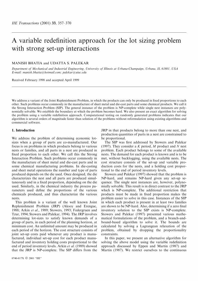
Stowers (1993) discusses the representation of theMULSP as a shortest path problem on a simple graph.The graph has a node Uk and node Vjk for each nest j. A¯ow of one unit entering node Uk, represents the satis-faction of demand through period k. Node Vjk representsthe nest chosen for production in period j while arcs�Vjk1 ;Uk2� represent production in period k1 using nest j tosatisfy demand through period k2 ÿ 1. Figure 1 shows thisgraph. It should be noted that, all extreme points of theMULSP polyhedron cannot be represented as a path inthis graph.We now discuss how to represent the MULSP as a

minimum cost network ¯ow problem, such that everyextreme point of the MULSP polyhedron corresponds toa feasible ¯ow in the network. Also, the MULSP variantwe consider can have a non-zero inventory in the ®nalperiod and the graph must be able to represent suchsolutions.We replace node Uk by two nodes U�ik and Uÿik , with

edge euik � �Uÿk ;U�k � between them, having a capacity ofone unit. All edges entering node Uk now enter node Uÿikand all edges leaving node Uk now leave U�ik . Flow of oneunit entering Uÿk represents satisfaction of demandthough period k. Set-up and production variables arerepresented separately by replacing node Vjk with nodes,V �ijk and V ÿijk, having edge evfijk � �V ÿijk; V �ijk� between them.Edge evfijk represents the set-up variable for family jin period k. Arc �Vjk;Ut� in the graph transformsto evuijkt � �V �ijk;U

ÿit �, and represents the production

variables. Similarly, edge �Vjk; L� transforms to edgeevlijk � �V �ijk; Li�.

To enable representation of extreme points involvingset-ups without production extra edges and nodes areneeded. Edges evbijk � �V �ijk; V

ÿijk� are added to the graph

to represent a production quantity of zero. Also, a``source'' node, Si, is added along with the edgesesvijk � �Si; V ÿijk� to allow extra set-ups to be made. Torepresent production in excess of the total demand,an extra node Wi is added to the graph. Edgesevwijk � �V �ijk;Wi� representing this excess production arealso added, along with the edge elwi � �Li;Wi� to com-plete the graph. Note that a ¯ow of one unit through edgeevwijk represents a production of Mijk units. To en-sure non-trivial ¯ows through the network, edgeesfi � �Si;Uÿi1 � is added and ¯ow through it is constrainedto be one. This edge represents the condition that at leastone family must be set-up in the ®rst period. Finally, edgeewsi � �Wi; Si� is added to complete the transformation toa minimum cost circulation problem. All edges in thenetwork, except edges elwi and ewsi are assigned acapacity of one unit. The resulting network for a twoperiod, two source problem is shown in Fig. 2.Formally, the MULSP can be represented by graph

G � �V;E�. The vertex set V consists of the followingedges

Si;Wi; Li 8 i; Uÿik ;U�ik 8 i; k and V ÿijk; V

�ijk 8 i; j; k:

The edge set E consists of the following edges.

esfi � �Si;U�i1 � 8 i; esvjk � �Si; V ÿijk� 8 i; j 2 Ji; k;

euik � �Uÿik ;U�ik � 8 i; k; euvijk � �U�ik ; V ÿijk� 8 i; j 2 Ji; k;

evfijk � �V ÿijk; V�

ijk� 8 i; j 2 Ji; k;

evbijk � �V �ijk; Vÿ

ijk� 8 i; j 2 Ji; k;

evuijkt � �V �ijk;Uÿit � 8 i; j 2 Ji; k; t > k;

evlijk � �V �ijk; Li� 8 i; j 2 Ji; k;

evwijk � �V �ijk;Wi� 8 i; j 2 Ji; k; elwi � �Li;Wi� 8 i;

ewsi � �Wi; Si� 8 i:

Fig. 1. MULSP network. Fig. 2. Modi®ed MULSP network.


All edges, except edges elwi and ewsi are assigned acapacity of one unit. Proposition 7 restricts Xijk to a ®niteset of values given by Cijk � Dit ÿ Di;kÿ1 for somet � k ÿ 1 or Xijk � Mijk. Hence, the above assignment ofcapacities does not eliminate any feasible solution.

3.3. The reformulated model

We now develop an alternative model for the SIP, usingthe network ¯ow representation of the MULSP, dis-cussed in the previous section. The transformation Tfrom the MULSP variables de®ned above to the variablescorresponding to region MP is given by

Yijk � evfijk 8 i; j; k; �20�Xijk�

Xt>k

Diktevuijkt�Dik;K�1evlijk�Mijkevwijk 8i;j;k: �21�

Then an alternate formulation for the SIP is given bymodel RP.

m�RP� � minX

i

Xj

Xk

cvfijkevfijk

�X

i

Xj

Xk

Xt>k

cvuijktevuijkt

�X

i

Xj

Xk

cvlijkevlijk

�X

i

Xj

Xk

cvwijkevwijk ÿ a; �22�

subject to

ewsi ÿ esfi ÿX

j

Xk

esvijk � 0 8 i; �23�

esfi ÿ eui1 � 0 8 i; �24�Xj2Ji

Xt<k

evuijtk ÿ euik � 0 8 i; k > 1; �25�

euik ÿXj2Ji

euvijk � 0 8 i; k; �26�

euvijk � esvijk � evbijk ÿ evfijk � 0 8 i; j 2 Ji; k; �27�evfijk ÿ evbijk ÿ

Xt>k

evuijkt ÿ evlijk ÿ evwijk � 0

8 i; j 2 Ji; k; �28�Xj2Ji

Xk

evlijk ÿ elwi � 0 8 i; �29�Xj2Ji

Xk

evwijk � elwi ÿ ewsi � 0 8 i; �30�

evfijk 2 f0; 1g 8 i; j 2 Ji; k; �31�Xt>k

Diktevuijkt � Dik;K�1evlijk �Mijkevwijk ÿ aijXjk � 0

8 j; i 2 Ij; k; �32�

evfi1jk ÿ evfi2jk � 0 8 j; i1; i2 2 Ij; k: �33�With the objective function coe�cients given by the fol-lowing equations.

cvfijk � Sjk

jIjj 8 i; j; k;

cvuijkt � Pijk�Di;tÿ1 ÿ Di;kÿ1� 8 i; j; k; t > k;

cvlijk � Pijk�DiK ÿ Di;kÿ1� 8 i; j; k;

cvwijk � Pijk�Mijk ÿ Di;kÿ1� 8 i; j; k:

Note that constraints (23)±(31) for a given i, are theusual network ¯ow constraints for the graph in Fig. 2 andde®ne the MULSP for product i. Also, constraints (32)and (33) correspond to the complicating constraints ofthe original model. Let NF be the region de®ned byconstraints (23)±(31), and let NF be the region de®ned byconstraints (23)±(30). Clearly, NF is the linear relaxationof NF . Also, since NF corresponds to a region de®ned bya network ¯ow problem, conv�NF � � NF .

Proposition 8. The set NF is strongly equivalent to MPunder transformation T de®ned by Equations (20) and (21).

Proof. By Proposition 7, we know that every extremepoint of conv�MP� is a feasible solution to NF , i.e., afeasible ¯ow through the set of MULSP networks for theM products. Also, every feasible solution to NF (a set offeasible ¯ows through the MULSP graphs) correspondsto a feasible solution to MP . Hence, the necessary andsu�cient conditions of strong equivalence (Martin, 1987)are satis®ed, and MP is strongly equivalent to NF underT . j

Note also that every feasible solution to NF correspondsto a feasible solution to MP . Using Propositions 2, 3 and8 we get the following results.

Proposition 9. If z is an optimal solution to problem RP,then Tz is an optimal solution to problem WP.

Proposition 10. The LP relaxation of model RP, yieldsbounds equal to those obtained by solving the LagrangeanDual with respect to constraints (7), i.e., m�RP � � maxl

�m�WPl��.Stowers and Palekar (1997) solve WPl, the Lagrangean

relaxation of problem WP with respect to constraints (7),to obtain the lower bounds in their branch and boundapproach. Note that problem WPl is a multi-nest JRP,with negative variable production costs. The multi-sourceJRP has been studied by Stowers (1993) and shown to beNP-complete. Thus the approach used by Stowers andPalekar (1997) involves solving a NP-complete problemat each node of the branch-and-bound tree to obtainlower bounds. Proposition 10 establishes that the LP


relaxation of formulation RP yields bounds at least asgood as those obtained by solving WPl. Also, thesebounds are obtained by solving an LP and are expected totake signi®cantly less time to calculate.

4. An enumerative approach for solving the SIP

In this section we present an enumerative approach forthe continuous production variant of the SIP. The pro-posed method is a branch-and-bound method, precededby some pre-processing of the problem. Pre-processinginvolves combining di�erent products into a single ag-gregate product and determining and eliminating ``re-dundant products''. Branching is achieved by ®xing theset-up variables. A depth-®rst strategy is ®rst used to ®ndan initial feasible solution, after which we switch to abreadth-®rst strategy. At each node the bounds are cal-culated by solving the LP relaxation of the model RP.Nodes are fathomed whenever the bounds exceed thevalue of a known feasible solution. We now presentmethods for pre-processing the problem to reduce theproblem size.

4.1. Product aggregation

Stowers and Palekar (1997) present a method of aggre-gating products unique to a family into one aggregateproduct. We extend this to the case where the productsare present in more than one family. The product ag-gregation procedure is formalized in the following prop-osition, which is stated without proof.

Proposition 11. Let i1 and i2 be two products such thatJi1 � Ji2 and

ai1j

ai2j� k 8 j 2 Ji1 ;

where k > 0 is a constant. Then products i1 and i2 can becombined into a single product õ with the following multi-plicities, demands and holding costs

aõj � ai1j 8 j 2 Ji1 ;

Dõk � max�Di1k; kDi2k� 8 k;

Hõk � Hi1k � 1

kHi2k 8 k:

For example, consider a two nest SIP with products 1and 2 belonging to both nests families having multiplicityone. Clearly, the demand for both products in period k issatis®ed i� X

t<k

�X1t � X2t� > max�D1k;D2k�:

Thus, the products can be considered as one aggregateproduct with holding cost equal to the sum of the holdingcosts, as given by Proposition 11.

4.2. Product dominance

Using Proposition (11), it may be possible to replace a setof products by an aggregate product. This proposition is,however, unlikely to be useful when the multiplicity ofproducts in the families varies randomly. We now de-velop another method for pre-processing the SIP, inwhich we attempt to identify products that are ``domi-nated'' by other products. These products can thenbe eliminated from the problem by suitably modifyingthe problem's cost structure. The following discussionformalizes this concept.

De®nition 1. Product i is said to be a Dominated Productif its demand in each period is bound to be satis®ed by theproduction required to satisfy the demand for the remainingproducts, due to the proportionality constraints.

Proposition 12. Product i1 is a Dominated Product, if thereexists solution to the following set of linear equations.X

i 6�i1

likaij

Dikÿ ai1j

Di1k� 0 8 j; k;

Xi6�i1

lik � 1 8 k;

lik � 0 8 i; k:

Proof. Note that constraints (2) can be written asXj

Xt�k

aij

DikXjk � 1 8 i; k: �34�

For every period k, we obtain the following validinequality, by taking a convex combination of theabove equations, with weight lik corresponding toproduct i.X

j

Xt�k

Xi6�i1

aijlik

Dik

!Xjk �

Xi6�i1

lik � 1:

The proof follows by comparing the coe�cients of thevariables in the above equation with those in constraints(34) for product i1. j

Proposition 13. Suppose product i1 is a Dominated Prod-uct in model P. Then an equivalent problem is obtained byremoving product i1 and modifying the cost of the produc-tion variables as follows.

Pjk � Vjk �Xi6�i1

Xt�k

aij�Hik � �iHi1k�;

where �i are the solution to the following system of linearequations

ai1j �Xi 6�i1

aij�i 8 j:


Proof. Let P1 and P2 be the problems before and aftereliminating product i1, using Proposition 13. The prob-lems have the same set of variables and only Equations(2) corresponding to product i1 are missing in P2. Theseconstraints are satis®ed by every solution feasible to P2,since i1 is a dominated product. Hence, the feasible regionfor both problems is the same. The two problems areequivalent if production costs are same, that is

Vjk �X

i

Xt�k

aijHik � Vjk �Xi 6�i1

Xt�k

aij�Hik � �iHi1k� 8 j; k;

which is true by choice of �i. Hence the two problems areequivalent. j

Propositions 11, 12 and 13 form the basis of the pre-processing subroutines that we develop. Note that thevalue of constant a is calculated using the initial data andis not changed after the pre-processing of the problem.The following example demonstrates the e�ectiveness ofthe pre-processing approach.

ExampleConsider a three-period SIP, with 10 products (numbered1±10) and four nests (labelled A±D). The multiplicities,aij, of the products and the demands are given in Table 1.Using Proposition 11, products 2 and 4 can be combinedinto a single aggregate product. Similarly, product setsf6;8g and f7;10g can each be combined into a singleaggregate product. This reduces the given instance to athree period, four nest and seven product probleminstance given in Table 2. The holding costs for theaggregate products in this case is the sum of the holdingcost for the individual products.We now identify and eliminate the dominated products

from the resulting problem, using Propositions 12 and 13.Consider products 1, 3 and 5 in this problem. Products 3and 4 belong to di�erent nests while product 1 is present inall the nests. Satisfying demand for products 3 and 4 en-sures that cumulative production of product 1 at end ofperiods 1, 2 and 3 is 92, 197 and 301 respectively. This

production is su�cient to satisfy the demand of product 1in the three periods. Thus, product 1 is a dominatedproduct and can be eliminated by distributing its holdingcost between the other products, in accordance withProposition 13. Similarly, we ®nd that products f2; 4g and9 are both dominated by product 5 and can be eliminatedfrom the problem. The problem, thus, reduces to a threeperiod, four nest and four product instance of the SIP,shown between the double horizontal lines in Table 2.Aggregation and elimination of products thus reduces theproblem size and is expected to result in considerable re-duction in the time required to solve the problem.

5. Computational experience

We now describe some computational experiments withthe approach described in Section 4. For the ®rst set oftest problems we use the same random test problemgenerator as the one used by Stowers and Palekar (1997).Problems generated by this generator are given the fourdigit code xxxx. The generator used by Stowers andPalekar restricts the multiplicity of the products in thenests to zero or one. Also, the total demand for theproducts is independent of the number of nests to which itbelongs. It is reasonable to assume that high demandproducts would be placed in a larger number of nests thanlow demand products. To overcome the above limitationsof the previous problem sets, we generate another set ofproblems in which the multiplicity is a random integerbetween zero and 10, and the demand is drawn from anormal distribution whose mean is proportional to thetotal multiplicity of the product in all families. The coststructure is similar to the one used by Stowers andPalekar (1997). These sets are given the code Mxxxx andare referred to as the high multiplicity problems.Stowers and Palekar (1997) compared the performance

of the Lagrangean relaxation approach to the LP relax-ation approach for problem sets xxxx. The Lagrangeanrelaxation approach was found to be signi®cantly fasterthan the LP relaxation approach. For the two nest

Table 1. Data set for a SIP instance

Product Multiplicity Demands

A B C D Di1 Di2 Di3

1 1 1 1 1 62 113 1722 1 1 1 . 47 96 1493 1 . . 1 42 94 1534 1 1 1 . 46 101 1445 . 1 . . 50 103 1486 . 1 1 . 54 104 1557 . . 1 1 42 101 1408 . 1 1 . 48 113 1679 . 1 1 1 46 101 15710 . . 1 1 54 99 150

Table 2. SIP instance after product aggregation

Product Multiplicity Demands

A B C D Di1 Di2 Di3

*1 1 1 1 1 62 113 172*{2,4} 1 1 1 . 47 96 1533 1 . . 1 42 94 1535 . 1 . . 50 103 148{6,8} . 1 1 . 54 113 167{7,10} . . 1 1 54 101 150*9 . 1 1 1 46 101 157

*: Dominated Products.Products 3,5,f6,8g & f7,10g left after Product Dominance.


problems (sets xx1x), the Lagrangean approach requiresfewer nodes and signi®cantly less time. The Lagrangeanapproach is 2±5 times faster than the LP relaxation ap-proach in most cases and between 7±10 times faster for afew sets. For the four nest problems (sets xx2x), the La-grangean approach is faster or can solve more problemsin most sets. For sets 1323, 2323 and 3323, the LPrelaxation approach is slightly faster. In view of theseresults, we compare the reformulation approach only tothe Lagrangean approach.To compare our reformulation method with the

Lagrangean approach of Stowers and Palekar (1997), we®rst solved all problems using both approaches. TheLagrangean approach involves using the product aggre-gation procedure proposed by Stowers and Palekar(1997) to pre-process the problem. This is followed by abranch-and-bound method to solve the problem. Thebounds are obtained by solving the Lagrangean relax-ation of problemWP with respect to constraints (8), usingthe optimal dual variable values from WP as the Lagrangemultipliers. IBM/OSL is used for the branch-and-bound,while the Lagrangean relaxation is solved using CPLEX.Our reformulation approach involves pre-processing theproblem using Propositions 11, 12 and 13 followed by thereformulation discussed in Section 3.3. IBM/OSL is thenused to solve the reformulated model, RP. We also usedthe OSL pre-processing subroutine EKKMPRE. Thissubroutine pre-processes the problem to generate validinequalities and tightens the formulation. It also ®ndsinitial heuristic solutions to the problem.Tables 3, 4 and 5 summarize the results of the tests for

sets xxxx. Computational times are reported in CPUseconds. Except for the Lagrangean approach for setsxxxx, all other problem sets are run on an IBM RS6000model 350 with 64 MB of RAM. For the Lagrangeanapproach for set xxxx, we use the results obtained byStowers and Palekar (1997) who solved these problems onan IBM RS6000 model 320 with 8 MB of RAM. Wesolve some problems on model 350 using the Lagrangeanapproach and observe that the times taken reduce, on theaverage, by a factor of 3.3.The average time for the Lagrangean approach is thus

reported as the time taken on IBM model 320 divided bya factor of 3.3. Note that Dongarra (1992) found thatmodel 350 is around 1.6 times faster than model 320 whilesolving dense systems of linear equations. The remainingdi�erence can be attributed to the di�erence in the size ofthe RAM.

5.1. Comparison of Root Node Lower Bounds

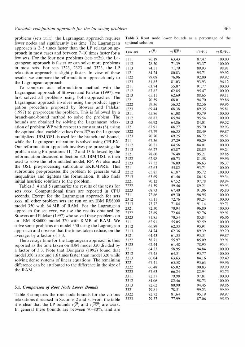
Table 3 compares the root node bounds for the variousrelaxations discussed in Sections 2 and 3. From the tableit is clear that the LP bounds m�P � and m�WP� are weak.In general these bounds are between 70±80%, and are

Table 3. Root node lower bounds as a percentage of theoptimal solution

Test set m(P) m(WP) m(WPl) m(RWPl)

1111 76.19 63.43 87.47 100.001112 78.30 71.39 93.37 100.001113 74.51 71.79 89.93 98.911121 84.24 80.83 95.71 99.921122 79.08 76.96 92.00 99.921123 81.85 81.03 93.93 96.121211 63.74 55.07 91.77 100.001212 67.82 62.85 95.47 100.001213 65.11 62.69 88.65 99.111221 70.59 68.01 94.70 99.861222 59.36 56.32 82.56 99.951223 69.44 68.38 89.35 95.811311 65.86 61.08 95.79 100.001312 68.87 65.94 95.54 100.001313 66.92 64.86 84.01 99.521321 67.91 66.27 95.70 99.931322 67.79 66.35 88.49 99.871323 70.70 69.25 86.72 95.512111 67.36 57.29 90.29 100.002112 70.21 64.56 84.01 100.002113 66.27 63.87 88.85 99.242121 78.60 76.48 95.21 99.852122 62.98 60.73 81.58 99.962123 77.52 76.09 96.63 96.372211 62.63 55.82 93.71 100.002212 65.85 61.87 95.72 100.002213 63.69 61.46 86.18 99.342221 70.12 67.52 97.78 99.942222 61.39 59.46 89.21 99.932223 68.73 67.40 91.06 95.802311 72.86 69.30 96.95 100.002312 75.11 72.76 98.24 100.002313 73.72 71.84 91.14 99.712321 72.30 70.94 96.80 100.002322 73.89 72.64 92.76 99.912323 71.85 70.54 85.84 96.063111 62.91 55.05 92.59 100.003112 66.89 62.33 95.91 100.003113 64.74 62.36 89.39 99.203121 64.43 61.33 93.31 99.873122 58.71 55.97 85.09 99.913123 62.44 61.48 78.95 95.443211 64.23 58.95 94.84 100.003212 67.45 64.31 95.77 100.003213 66.04 63.63 84.16 99.493221 67.41 65.58 95.63 99.963222 66.48 65.02 90.83 99.903223 67.63 66.24 82.94 95.753311 82.37 79.98 97.81 100.003312 84.06 82.46 98.73 100.003313 82.62 80.90 94.45 99.863321 79.81 78.51 99.23 99.993322 82.72 81.64 95.19 99.973323 79.37 77.99 87.06 95.50


always less than 90%, of the optimal solution. TheLagrangean bounds m�WPl� represent a signi®cantimprovement over these bounds. The Lagrangean boundsare usually about 5±20% larger, and as much as 30%larger in some cases.The reformulation bounds, m�RP�, are even stronger.

The bounds are usually 3 to 10% more than the La-grangean bounds, and up to 15±18% more in some cases.The maximum improvement is observed in the test sets ofthe form xx13 and xx22. The improvement is usually morethan 10%, and is as high as 17% in sets 1222 and 2122. Ingeneral, the reformulation bounds are more than 99%,and are never less than 95% of the optimal solution. Infact, the bounds are less than 99% only for test sets of theform xx23. These are problems with four nests and a highproduct density in nests and are expected to be moredi�cult to solve.

5.2. Comparison of low multiplicity problems (xxxx)

Table 4 shows the results obtained after solving all testproblems to optimality. These results are even more im-pressive than the root node bounds. With the use of m�RP�as bound, we have signi®cantly reduced the time taken tosolve the problems. Also, the number of nodes exploredin the branch-and-bound tree is greatly reduced. This isimportant because weak bounds result in large trees andout of memory errors. Strong bounds thus allow moreproblems to be solved.The reformulation approach solves all problems in all

sets. Except for the problem sets of the form xx23, it takesless than 30 nodes and less than 4 seconds to solve theproblems. In general, the average time taken is less than2 seconds. Also, all problems in as many as 23 of the 54sets are solved to optimality at the root node. The truee�ectiveness of the approach, however, is seen only whencompared with the results of the Lagrangean approach.Unlike the reformulation approach, the Lagrangean

approach is unable to solve all the problems. For somesets it solves as few as one problem. Moreover, it requiressigni®cantly more time to do so. Consider test set 2221for example. The Lagrangean approach solves only oneproblem in the set, taking 627 seconds and 13 720 nodes.The reformulation approach solves all ®ve problems,taking an average of 0.93 seconds and an average of 1.6nodes. Similar results are obtained for the problem set2121. The Lagrangean approach solves one problem,taking 526 seconds and 8554 nodes. The reformulationapproach solves all ®ve problems, taking an average of0.99 seconds and 4.4 nodes. Sets 1222, 2222, 3121 and3122 also show similar results. The reformulation ap-proach requires less than 2.6 seconds and 18 nodes tosolve these sets, while the Lagrangean approach requiresmore than 1600 nodes and 340 seconds.The reformulation approach shows the poorest results

for the sets of the form xx23. Notice that it is for these

Table 4. Comparison of all problems solved to optimality formodel P

Totalset

Reformulationapproach

Lagrangean relaxationapproach

Solved Numberof

nodes

Averagetime

Solved Numberof

nodes

Averagetime

1111 5 0.00 0.12 5 90.00 3.081112 5 0.00 0.11 5 186.40 7.381113 5 8.40 0.76 5 108.40 9.331121 5 1.60 0.92 5 1626.80 83.751122 5 0.00 1.94 5 5254.80 384.651123 5 5646.60 599.67 3 2151.33 329.931211 5 0.00 0.11 5 1356.00 40.121212 5 0.00 0.11 5 3038.00 133.061213 5 16.00 0.82 5 1006.40 75.751221 5 7.20 1.07 3 10 641.33 623.151222 5 2.40 2.16 2 8744.00 648.891223 5 4907.80 935.86 1 3969.00 1701.571311 5 0.00 0.11 5 92.60 3.661312 5 0.00 0.11 5 150.20 7.921313 5 7.60 0.60 5 116.20 11.031321 5 6.80 1.09 5 3540.40 209.441322 5 22.20 3.92 5 1524.80 135.031323 5 230.20 59.17 3 495.33 122.842111 5 0.00 0.12 5 732.40 20.642112 5 0.00 0.11 5 4813.80 208.892113 5 20.40 1.03 5 4013.00 293.592121 5 4.40 0.99 2 8554.00 525.782122 5 1.60 2.20 1 1944.00 178.652123 5 12 290.80 1896.02 1 11 497.00 993.382211 5 0.00 0.12 5 642.00 19.302212 5 0.00 0.11 5 1067.60 51.692213 5 11.60 0.67 5 749.60 73.522221 5 1.60 0.93 1 13 720.00 626.912222 5 7.60 2.53 3 7667.67 775.512223 5 863.00 185.84 3 7900.33 1308.562311 5 0.00 0.11 5 17.60 1.392312 5 0.00 0.10 5 20.00 2.072313 5 0.80 0.39 5 26.60 4.302321 5 0.00 0.40 5 277.60 17.752322 5 10.80 2.54 5 74.00 9.022323 5 30.80 13.19 5 413.20 159.323111 5 0.00 0.12 5 1084.40 31.663112 5 0.00 0.12 5 1802.20 84.813113 5 4.80 0.56 5 1083.80 89.223121 5 17.20 1.39 2 17 065.00 990.483122 5 4.00 2.35 2 3967.50 340.093123 5 3814.20 757.47 3 5994.67 2236.783211 5 0.00 0.12 5 166.60 5.833212 5 0.00 0.11 5 282.20 15.093213 5 7.60 0.61 5 160.80 18.163221 5 4.40 0.96 5 5773.40 356.403222 5 10.00 3.80 5 4195.60 338.583223 5 177.20 51.54 4 2582.00 1226.743311 5 0.00 0.11 5 3.20 0.833312 5 0.00 0.11 5 0.80 1.063313 5 0.00 0.31 5 0.00 2.07


very sets that the root node bound is weakest. Even forthese sets, the performance is favorable when comparedto the Lagrangean approach. However for the problemsets 1123 and 2123, the average time required is more thanthe Lagrangean approach. This is due to the fact that theLagrangean approach solves only a few of the ``easier''problems in these sets. Table 5 compares only thoseproblem instances that both strategies are able to solve tooptimality. We then ®nd that the reformulation approachtakes less time than the Lagrangean approach for all sets.For example consider set 2123. From Table 4 we see thatthe reformulation approach solves all the problems takingan average of 1896 seconds, while the Lagrangean ap-proach solves one problem taking 993 seconds. If we nowcompare the problem that both methods solved, we ®ndthat the reformulation method requires only 1.33 secondscompared to the 993 seconds that the Lagrangeanapproach takes. This problem is solved to optimality atthe root node by the reformulation approach, while theLagrangean approach requires 11 497 nodes.It was noticed that problem instances in set xx23, which

were di�cult to solve, exhibited the nest structure shownin Table 6. Viewed as a node-arc incidence matrix,the nest matrix reveals a cycle. In this case, each productcan be produced using two nests and each nest producestwo products. Assuming constant demand, d, for allproducts in each period, the optimal LP solution to theproblem is

Yjk � 0:5 8 j; k and Xjk � d28 i; k:

The optimal IP solution to the same problem is

Yjk � 1 8 j 2 fA;Bg; k odd YCk � 1 8 k even;

Xjk � dYjk 8 j; k:

Thus, the optimal LP solution has the same set-up cost asthe optimal IP solution, but saves on the holding cost.The di�culty in solving the problem can be attributed tothe highly fractional LP solutions caused by this neststructure.

Table 5. Comparison of problems solved to optimality by bothmethods for model P

Testset

Comparisons Reformulationapproach


Numberof

nodes

Averagetime

Numberof

Nodes

Averagetime

1111 5 0.00 0.12 90.00 3.081112 5 0.00 0.11 186.40 7.381113 5 8.40 0.76 108.40 9.331121 5 1.60 0.92 1626.80 83.751122 5 0.00 1.94 5254.80 384.651123 3 93.33 16.57 2151.33 329.931211 5 0.00 0.11 1356.00 40.121212 5 0.00 0.11 3038.00 133.061213 5 16.00 0.82 1006.40 75.751221 3 12.00 1.54 10 641.33 623.151222 2 6.00 4.62 8744.00 648.891223 1 24.00 9.69 3969.00 1701.571311 5 0.00 0.11 92.60 3.661312 5 0.00 0.11 150.20 7.921313 5 7.60 0.60 116.20 11.031321 5 6.80 1.09 3540.40 209.441322 5 22.20 3.92 1524.80 135.031323 3 59.33 14.31 495.33 122.842111 5 0.00 0.12 732.40 20.642112 5 0.00 0.11 4813.80 208.892113 5 20.40 1.03 4013.00 293.592121 2 11.00 1.91 8554.00 525.782122 1 8.00 7.80 1944.00 178.652123 1 0.00 1.33 11 497.00 993.382211 5 0.00 0.12 642.00 19.302212 5 0.00 0.11 1067.60 51.692213 5 11.60 0.67 749.60 73.522221 1 0.00 0.35 13 720.00 626.912222 3 12.67 3.92 7667.67 775.512223 3 100.67 19.82 7900.33 1308.562311 5 0.00 0.11 17.60 1.392312 5 0.00 0.10 20.00 2.072313 5 0.80 0.39 26.60 4.302321 5 0.00 0.40 277.60 17.752322 5 10.80 2.54 74.00 9.022323 5 30.80 13.19 413.20 159.323111 5 0.00 0.12 1084.40 31.663112 5 0.00 0.12 1802.20 84.813113 5 4.80 0.56 1083.80 89.223121 2 0.00 0.33 17 065.00 990.483122 2 10.00 5.05 3967.50 340.093123 3 2460.67 396.87 5994.67 2236.783211 5 0.00 0.12 166.60 5.833212 5 0.00 0.11 282.20 15.093213 5 7.60 0.61 160.80 18.163221 5 4.40 0.96 5773.40 356.403222 5 10.00 3.80 4195.60 338.583223 4 84.00 32.52 2582.00 1226.743311 5 0.00 0.11 3.20 0.833312 5 0.00 0.11 0.80 1.063313 5 0.00 0.31 0.00 2.07

Table 4. (Continued)

Totalset



Solved Numberof

nodes

Averagetime

Solved Numberof

nodes

Averagetime

3313 5 0.00 0.31 5 0.00 2.073321 5 0.00 0.67 5 14.80 2.713322 5 0.00 1.65 5 10.40 3.663323 5 12.80 8.69 5 60.00 18.85

Product multiplicity, aij 2 f0; 1g.


5.3. Comparison of high multiplicity problems (Mxxxx)

The results for the problem sets Mxxxx are summarized inTables 7 and 8, and are similar to the previous results.These are problems in which product multiplicity in thenest varies randomly. The reformulation approach solvesall problems in most sets, while the Lagrangean approachis unable to solve any in as many as 20 sets. The refor-mulation approach continues to perform better than theLagrangean approach in terms of both bounds and times.Consider for example set M3323. The reformulation ap-proach solves all problems taking an average of 55 sec-onds and 51 nodes, while the Lagrangean approach isunable to solve any problem. Similar results are obtainedfor sets M312x, M222x and M122x. Consider sets M121x.While the reformulation approach takes less than 8 sec-onds and 15 nodes, the Lagrangean approach takes 430±1329 seconds and 10 700±18 600 nodes. Similar resultsare seen for the sets M131x, M221x, M311x and M321x.For all sets where comparisons are possible, the refor-mulation approach takes less time and nodes and solvesmore problems than the Lagrangean approach. Table 8compares the problems solved to optimality by bothmethods. The results are similar to those discussed above.

6. Conclusion

In this paper we considered a variant of the Joint Re-plenishment Problem in which parts can only be pro-duced in ®xed proportion to each other. We present areformulation-based approach to solve the problem tooptimality. Computational experiments show that theapproach performs well when compared to existingalgorithms and a standard optimization package.


Testset



Numberof

nodes

Averagetime

Numberof

Nodes

Averagetime

3321 5 0.00 0.67 14.80 2.713322 5 0.00 1.65 10.40 3.663323 5 12.80 8.69 60.00 18.85

Product multiplicity, aij 2 f0; 1g.

Table 6. Nest structure of xx23 problems

Nests Products

P1 P2 P3

A 1 . 1B 1 1 .C . 1 1

Table 7. Comparison of problems solved to optimality formodel P

Testset



Solved Numberof nodes

Averagetime


Averagetime

M1111 5 6.00 2.16 5 247.20 7.88M1112 5 20.80 4.91 5 694.40 32.33M1113 5 111.20 12.32 5 2879.00 179.54M1121 5 432.40 31.06 3 62 498.00 5100.90M1122 5 19 084.00 2336.37 0 DNS DNSM1123 1 10 176.00 1196.82 0 DNS DNSM1211 5 10.80 2.51 5 10 745.20 429.64M1212 5 10.40 4.24 5 14 056.40 707.84M1213 5 14.80 7.34 5 18 610.40 1329.03M1221 5 418.20 33.02 0 DNS DNSM1222 5 11 494.60 1869.29 0 DNS DNSM1223 3 5289.00 2598.55 0 DNS DNSM1311 5 2.00 1.34 5 7287.40 299.41M1312 5 4.40 1.95 5 5987.00 339.86M1313 5 2.40 4.64 5 4879.80 338.77M1321 5 95.60 17.49 1 26 396.00 1282.84M1322 5 540.00 169.39 0 DNS DNSM1323 5 1460.80 1299.41 0 DNS DNSM2111 5 60.40 3.79 5 1956.20 60.64M2112 5 110.80 8.79 5 5582.80 244.73M2113 5 69.60 11.82 5 14 755.40 979.57M2121 5 568.40 39.22 0 DNS DNSM2122 3 4522.33 389.25 0 DNS DNSM2123 2 9081.00 1916.79 0 DNS DNSM2211 5 4.80 2.28 5 8882.20 355.55M2212 5 7.20 3.74 5 13 702.40 833.01M2213 5 7.20 5.79 5 16 748.40 1209.06M2221 5 69.00 14.03 0 DNS DNSM2222 5 3183.40 640.14 0 DNS DNSM2223 5 8755.40 4579.73 0 DNS DNSM2311 5 0.00 1.15 5 2226.20 79.61M2312 5 3.20 2.64 5 1887.20 93.74M2313 5 3.60 5.02 5 1287.00 84.89M2321 5 38.80 10.57 2 6310.00 337.43M2322 5 120.80 54.22 1 82 699.00 11 521.68M2323 5 207.80 193.55 0 DNS DNSM3111 5 7.20 2.52 4 12 682.25 527.33M3112 5 4.40 3.20 5 12 667.80 709.01M3113 5 11.60 6.95 5 18 583.80 1397.98M3121 5 120.60 17.45 0 DNS DNSM3122 5 5730.40 961.30 0 DNS DNSM3123 5 14 529.20 6249.15 0 DNS DNSM3211 5 3.20 1.48 5 8117.20 346.01M3212 5 3.20 2.59 5 8858.60 486.04M3213 5 4.00 3.96 5 7229.20 521.89M3221 5 51.00 13.77 1 32 622.00 1743.98M3222 5 911.40 248.44 0 DNS DNSM3223 5 1340.40 1074.73 0 DNS DNSM3311 5 0.60 1.18 5 438.00 15.65M3312 5 0.60 1.55 5 393.20 19.33M3313 5 1.40 2.29 5 296.00 18.07M3321 5 23.60 8.34 4 12 648.75 877.76


References

Aksoy, Y. and Erenguc, S.S. (1988) Multi-item inventory models withco-ordinated replenishments. International Journal of Operationsand Production Management, 8, 63±73.

Arkin, E., Joneja, D. and Roundy, R. (1989) Computational com-plexity of uncapacitated multi-echelon production planningproblems. Operations Research Letters, 8, 61±66.

Dongarra, J.J. (1992) Computational complexity of uncapacitatedmulti-echelon production planning problems. Technical report,Computer Science Department, University of Tennessee, Knox-ville, TN.

Eppen, G.D. and Martin, R.K. (1987) Solving multi-item capactitatedlot-sizing problem using variable rede®nition. Operations Re-search, 35(6), 832±848.

Federgruen, A. and Tzur, M. (1994) The joint replenishment problemwith time varying costs and demands: e�cient asymptotic and �optimal solutions. Operations Research, 37, 909±925.

Gilmore, P.C. and Gomory, R.E. (1963) A linear programming ap-proach to the cutting stock problem: part ii. Operations Research,11, 863±888.

Martin, R.K. (1987) Generating alternate mixed-integer programmingmodels using variabe rede®nition. Operations Research, 35(6),820±831.

Stowers, C.L. (1993) Uncapacitated lotsizing problems with setup in-teractions. PhD thesis, Department of Mechanical and IndustrialEngineering, University of Illinois at Urbana-Champaign, IL.

Stowers, C.L. and Palekar, U.S. (1994) A dual ascent procedure for thejoint replinishment problem. Technical report, Department ofMechanical and Industrial Engineering, University of Illinois atUrbana-Champaign, IL.

Stowers, C.L. and Palekar, U.S. (1997) Lotsizing problems with strongset-up interactions. IIE Transactions, 29, 167±179.


Testset




Averagetime


Averagetime

M3322 5 65.60 26.27 2 23 953.00 2286.80M3323 5 50.40 54.49 0 DNS DNS

Product multiplicity, aij 2 f0; 10g.DNS: Did Not Solve Any Problem to Optimality.

Table 8. Comparison of problems solved to optimality by bothmethods for model P

Testset


Lagrangeanrelaxationapproach

Numberof

nodes

Averagetime

Numberof

nodes

Averagetime

M1111 5 6.00 2.16 247.20 7.88M1112 5 20.80 4.91 694.40 32.33M1113 5 111.20 12.32 2879.00 179.54M1121 3 490.67 36.46 62 498.00 5100.90M1122 0 NC NC NC NCM1123 0 NC NC NC NCM1211 5 10.80 2.51 10 745.20 429.64M1212 5 10.40 4.24 14 056.40 707.84M1213 5 14.80 7.34 18 610.40 1329.03M1221 0 NC NC NC NCM1222 0 NC NC NC NCM1223 0 NC NC NC NCM1311 5 2.00 1.34 7287.40 299.41M1312 5 4.40 1.95 5987.00 339.86M1313 5 2.40 4.64 4879.80 338.77M1321 1 108.00 21.06 26 396.00 1282.84M1322 0 NC NC NC NCM1323 0 NC NC NC NCM2111 5 60.40 3.79 1956.20 60.64M2112 5 110.80 8.79 5582.80 244.73M2113 5 69.60 11.82 14 755.40 979.57M2121 0 NC NC NC NCM2122 0 NC NC NC NCM2123 0 NC NC NC NCM2211 5 4.80 2.28 8882.20 355.55M2212 5 7.20 3.74 13 702.40 833.01M2213 5 7.20 5.79 16 748.40 1209.06M2221 0 NC NC NC NCM2222 0 NC NC NC NCM2223 0 NC NC NC NCM2311 5 0.00 1.15 2226.20 79.61M2312 5 3.20 2.64 1887.20 93.74M2313 5 3.60 5.02 1287.00 84.89M2321 2 27.00 7.22 6310.00 337.43M2322 1 112.00 29.32 82 699.00 11 521.68M2323 0 NC NC NC NCM3111 4 9.00 3.13 12 682.25 527.33


Testset


Lagrangeanrelaxationapproach

Numberof

nodes

Averagetime

Numberof

nodes

Averagetime

M3112 5 4.40 3.20 12 667.80 709.01M3113 5 11.60 6.95 18 583.80 1397.98M3121 0 NC NC NC NCM3122 0 NC NC NC NCM3123 0 NC NC NC NCM3211 5 3.20 1.48 8117.20 346.01M3212 5 3.20 2.59 8858.60 486.04M3213 5 4.00 3.96 7229.20 521.89M3221 1 111.00 21.75 32 622.00 1743.98M3222 0 NC NC NC NCM3223 0 NC NC NC NCM3311 5 0.60 1.18 438.00 15.65M3312 5 0.60 1.55 393.20 19.33M3313 5 1.40 2.29 296.00 18.07M3321 4 17.50 7.49 12 648.75 877.76M3322 2 95.00 22.57 23 953.00 2286.80M3323 0 NC NC NC NC

Product multiplicity, aij 2 f0; 10g.NC: No Comparisons Possible.


Wagner, H.M. and Whitin, T.M. (1958) Dynamic version of the eco-nomic lot size model. Management Science, 23, 89±96.

Zangwill, W.I. (1969) A deterministic multi-period production sched-uling model with backlogging. Management Science, 15, 506±527.

Appendix A: Proofs

Proposition 4. Every extreme point of conv�MPi� satis®esIi;kÿ1 � Xijk � �Mijk ÿ Xijk� � 0 8 j; k:

Proof. Note that since the initial inventory is assumed tobe zero, Equations (18) are satis®ed for k � 1. Suppose 9an extreme point li � �xi; yi� such that (18) is violated forj � j2 and k � k2 > 1. Let k1 be the last period before k2 inwhich product i was produced and let j1 be the nest used.If Xij1k1 < Mij1k1 let

u1 � u2 � minfIi;k2ÿ1;Xij1k1 ;Mij1k1 ÿ Xij1k1 ;Xij2k2 ;Mij2k2

ÿ Xij2k2g:If Xij1k1 � Mij1k1 let

u1 � 0; u2 � minfXij2k2 ;Mij2k2 ÿ Xij2k2g:Since (18) is violated, u2 > 0. De®ne l1

i � �x1i ; y1i � andl2

i � �x2i ; y2i � as follows:y1i � y2i � yi;

X 2ijk � X 1

ijk � Xijk 8 �j; k� 62 f�j1k1�; �j2k2�g;X 1

ij1k1 � Xij1k1 � u1; X 2ij1k1 � Xij1k1 ÿ u1;

X 1ij2k2 � Xij2k2 ÿ u2; X 2

ij2k2 � Xij2k2 � u2:

Note that production of Mijk units of product i is su�-cient to meet its demand in all subsequent periods. Hence,by the de®nition of u1 and u2 both l1

i and l2i are feasible

to conv�MPi�. Also, li � 12 �l1

i � l2i � which contradicts the

assumption that li was an extreme point. j

Proposition 6. Let li � �xi; yi� be an extreme point ofconv�MPi� and let k�i� be the ®rst period in whichXijk � Mijk for some j 2 Ji. Then Ii;k�i�ÿ1 � 0. Further,

Xijk 2 f0;Mijkg 8 j 2 Ji; k � k�i�:

Proof. Suppose 9 an extreme point li that violates theabove proposition, that is Ii;k�i�ÿ1 > 0 where k�i� is asde®ned above. Clearly k�i� > 1. Let k1 < k�i� be the lastperiod, before k�i�, in which product i was produced andlet j1 be the nest used. By de®nition of k�i� and k1,Xij1k1 < Mij1k1 . Let u � min�Xij1k1 ;Mij1k1 ÿ Xij1k1 ; Ii;k�i�ÿ1�.De®ne l1

i � �x1i ; y1i � and l2i � �x2i ; y2i � as follows:

y1i � y2i � yi;

X 2ijk � X 1

ijk � Xijk 8 �j; k� 6� �j1; k1�;X 1

ij1k1 � Xij1k1 � u; X 2ij1k1 � Xij1k1 ÿ u:

By de®nition of u, both l1i and l2

i are feasible solutionof conv�MPi�. Also, li � �l1

i � l2i �=2 which contradicts

the assumption that li is an extreme point of conv�MPi�.Note that if Xijk � Mijk for some k, thenIit > 0 8 t � k; . . . ;K ÿ 1. Equation (19) follow fromPropositions 4 and 5 and the de®nition of k(i). j

Proposition 7. Let li � �xi; yi� be a feasible solution toconv�MPi�. Then, li is an extreme point if and only if

1. Ii;kÿ1 � Xijk � �Mijk ÿ Xijk� � 0 8 j; k.2. Let Jik � fjjXijk > 0g. If jJik j > 1 then Xijk �

Mijk 8 j 2 Jik; k.3. Let k�i� be the ®rst period in which Xijk � Mijk for

some j 2 Ji. Then Ii;k�i�ÿ1 � 0.4. Yijk 2 f0; 1g 8 j; k.

Proof. Suppose 9 an extreme point li that violates theabove proposition, that is Ii;k�i�ÿ1 > 0 where k�i� is asde®ned above. Clearly k�i� > 1. Let k1 < k�i� be the lastperiod, before k�i�, in which product i was produced andlet j1 be the nest used. By de®nition of k�i� and k1,Xij1k1 < Mij1k1 . Let u � min�Xij1k1 ;Mij1k1 ÿ Xij1k1 ; Ii;k�i�ÿ1�.De®ne l1

i � �x1i ; y1i � and l2i � �x2i ; y2i � as follows:

y1i � y2i � yi;

X 2ijk � X 1

ijk � Xijk 8 �j; k� 6� �j1; k1�;X 1

ij1k1 � Xij1k1 � u; X 2ij1k1 � Xij1k1 ÿ u:

By de®nition of u, both l1i and l2

i are feasible solutionof conv�MPi�. Also, li � �l1

i � l2i �=2 which contradicts

the assumption that li is an extreme point of conv�MPi�.Note that if Xijk � Mijk for some k, then Iit > 0 8 t � k;. . . ;K ÿ 1. Equation (19) follow from Propositions 4 and5 and the de®nition of k(i). j

Biographies

Manish Bhatia received his B.Tech in Mechanical Engineering fromIIT-Delhi, India in 1994. He received an M.S. in Industrial Engineeringand a M.S. in Computer Science at the University of Illinois at Ur-bana-Champaign in 1996 and 1998 respectively. His research interestsare in production planning, optimization and software development.He currently resides in Pune, India where he works on softwaredevelopment and testing.

Udatta S. Palekar is an Associate Professor in the Department ofMechanical and Industrial Engineering at the University of Illinois atUrbana-Champaign. He received his B.E. in Production Engineeringfrom University of Bombay, India in 1982 and his M.S. and Ph.D.from the State University of New York at Bu�alo in 1984 and 1986respectively. He has research interests in the areas of supply chain andlogistics, production planning, location theory and combinatorialoptimization. He has also served as the Chairman of the TechnicalExecutive Committee of the ASME Material Handling Division.

Contributed by the Production Planning Department


Documents

A variable redefinition approach for the lot sizing problem with strong set-up interactions