A VaR-based optimal reinsurance model: the perspective of

Master’s Degree programmein Economics

Final Thesis

A VaR-basedoptimal reinsurance model:the perspective of both theinsurer and the reinsurer

SupervisorCh. Prof. Paola Ferretti

Assistant SupervisorCh. Prof. Stefania Funari

GraduandFederica Maria CogoMatriculation number 859273

Academic Year2016/2017

CONTENTS

Contents i

Introduction iii

1 Reinsurance: an overview 1

1.1 Introduction . . . . . . . . . . . . . . . . . . . . . . . . . . . . . . . . 1

1.2 Types of reinsurance . . . . . . . . . . . . . . . . . . . . . . . . . . . 2

1.2.1 Proportional Reinsurance . . . . . . . . . . . . . . . . . . . . 2

1.2.2 Non Proportional Reinsurance . . . . . . . . . . . . . . . . . 4

1.3 Costs and benefits of reinsurance . . . . . . . . . . . . . . . . . . . . 6

1.3.1 Solvency II . . . . . . . . . . . . . . . . . . . . . . . . . . . . . 8

2 The perspective of the insurer 11

2.1 Outline of the model and relevant literature . . . . . . . . . . . . . . 11

2.2 Preliminary conditions . . . . . . . . . . . . . . . . . . . . . . . . . . 12

2.2.1 Class of admissible Premium Principles . . . . . . . . . . . . 15

2.2.2 VaR Risk Measure . . . . . . . . . . . . . . . . . . . . . . . . . 18

2.3 A VaR minimization model . . . . . . . . . . . . . . . . . . . . . . . 20

2.4 Conclusions . . . . . . . . . . . . . . . . . . . . . . . . . . . . . . . . 25

3 The perspective of the reinsurer 27

3.1 Topic of research and existing literature . . . . . . . . . . . . . . . . 27

3.2 The optimization problem of the reinsurer . . . . . . . . . . . . . . . 28

i

ii CONTENTS

3.2.1 Different solutions for the two agents . . . . . . . . . . . . . 28

3.2.2 An optimal solution for the reinsurer . . . . . . . . . . . . . . 31

3.3 A comparative analysis of the results . . . . . . . . . . . . . . . . . . 36

3.4 Conclusions . . . . . . . . . . . . . . . . . . . . . . . . . . . . . . . . 39

4 The perspective of both 43

4.1 Multi-objective Optimization . . . . . . . . . . . . . . . . . . . . . . 43

4.1.1 Cai, Lemieux and Liu (2015): the weighted-sum method . . 47

4.1.2 Lo (2017): the ε-constraint method . . . . . . . . . . . . . . . 51

4.2 Conclusions and future research suggestions . . . . . . . . . . . . . 54

Conclusions 55

References 57

INTRODUCTION

Reinsurance is usually defined as «insurance for insurers»: under a reinsurance ar-

rangement, the reinsurer agrees on being transferred a portion of the risks under-

written by an insurance company, the so-called cedant. In exchange, the reinsurer

is paid a premium.

In recent decades, reinsurance has often been addressed in economic research:

the main objective is to determine the optimal form and level of reinsurance,

under either the perspective of the cedant, of the reinsurer or both. Specifically,

in light of the major role played by risk measures in the insurance regulatory

system, latest research has focused on risk-measure-based reinsurance models.

In particular, Cai and Tan (2007) were among the first to propose an optimal

reinsurance model, which explicitly employed the Value-at-Risk (VaR) risk mea-

sure in its objective function. The authors determined the level of retention, in a

stop-loss reinsurance, that minimizes the VaR of the total exposure of the cedant:

in this sense, it is optimal (see [2]). In 2011 and 2013, Chi and Tan further investi-

gated the model: by relaxing some of the original assumptions, they managed to

provide it with significant robustness (see [4, 5]).

The aim of this thesis is to study the model in Chi and Tan (2013), under

the different perspectives of the two parties involved in a reinsurance contract.

After an analysis of the VaR-based optimal reinsurance model from the cedant’s

point of view, the same is evaluated under the reinsurer’s one: our interest is

to determine whether and how the optimal reinsurance contract for the cedant

diverges from the one optimal for the reinsurer. In conclusion, the two agents’

iii

iv INTRODUCTION

antithetical perspectives are considered simultaneously: to the purpose, a field of

mathematics called Multi-Objective Optimization is introduced.

The structure of the thesis is as follows. In Chapter 1, an overview to reinsur-

ance is presented: in particular, we explain what it is and how and why it should

be used by insurance companies. In Chapter 2, we propose the model solved in

Chi and Tan (2013): after an exhaustive analysis of the set of preliminary con-

ditions, the main theorem is formalized and proved step-by-step. In Chapter 3,

we focus on the perspective of the reinsurer: under the same assumptions, we

study whether the reinsurance contract, proved optimal in Chapter 2, might be

optimal also for the reinsurer; since it is not, we look for a different reinsurance

policy, which minimizes the VaR of the reinsurer’s total risk exposure. In Chapter

4, Multi-objective Optimization is introduced: first, we explain why it might be

used to formalize an optimal reinsurance model, capable of taking into account

both agents’ conflicting interests; then, we show how Cai, Lemieux and Liu (2015)

and Lo (2017) resorted to two different Multi-objective Optimization methods to

derive mutually acceptable optimal solutions.

CHAPTER 1

REINSURANCE: AN OVERVIEW

1.1 Introduction

Non-life insurers usually face fortuitous claims experiences, which threaten the

results of their portfolios and may consequently impinge on their overall perfor-

mances and capitals (see [1]). In example, an unforeseen catastrophe may affect

multiple risks in the same portfolio and lead to a major total loss; or frequent

small losses might result in an overall burden far greater than expected. As a

consequence, the only way to ensure stable results is through diversification. By

the nature of their business, though, insurers do not have the means, nor the pos-

sibility, to maximally diversify the risks they hold. A valid solution is offered by

reinsurance.

Reinsurance is a form of risk sharing, usable as a risk mitigating tool: buying

reinsurance cover for a given premium, the insurer (cedant) can transfer part

of its risk to the reinsurer. The latter, operating worldwide and across different

lines of business, can exploit diversification to achieve a more efficient use of its

capital, which is translated into capital relief for the cedant. Also, resorting to

reinsurance, the cedant gains the possibility to underwrite a larger number of

risks, improving its position in the market and spreading, and potentially better

diversifying, its portfolios.

1

2 CHAPTER 1. REINSURANCE: AN OVERVIEW

1.2 Types of reinsurance

The offerings of reinsurance covers are as varied as the different and evolving

needs of insurers. There exists both Facultative Reinsurance, which can be bought

to ensure protection against major single risks, and Treaty reinsurance, which cov-

ers entire portfolios. According to how much time claims might take to be settled,

it is also possible to choose between Short-Tail Reinsurance or Long-Tail Reinsur-

ance. In some business segments claims are usually settled within a short period

(i.e. property lines): in these cases, Short-Tail Reinsurance is suggested. In oth-

ers, years or decades may pass before claims are paid off (i.e. liabilities lines): for

these, Long-Tail Reinsurance is suitable. Also, the cedant can choose whether to

buy a Direct Reinsurance, without an intermediary, or a Brokered Reinsurance (see

[11]). The main difference, though, is between Proportional and Non-Proportional

Reinsurance.

1.2.1 Proportional Reinsurance

With a proportional reinsurance treaty, also known as Pro Rata Reinsurance, the

cedant proportionally shares one or more of its policies with the reinsurer, paying

a percentage of the received premiums: in exchange, the reinsurer complies with

underwriting the same proportion of the risks and paying the relative claims.

It follows a brief description of the main characteristics of the two more com-

mon kinds of Proportional Reinsurance (see [6, 1]).

Quota Share Reinsurance

• A Quota Share reinsurance allows the cedant to cede to the reinsurer a fixed

proportion of all the policies, within the scope of the Treaty.

• The net amount of risk the insurer agrees to keep for its own account is

defined as retention. In this case, the cedant retains a fixed percentage and

the reinsurer bears the exceeding quota share.

1.2. TYPES OF REINSURANCE 3

• Underwriting the risks, the reinsurer accepts all the conditions originally

agreed between the policyholder and the direct insurer.

• It is usual to agree on an absolute quota share limit, to within the potential

loss the reinsurer may be burdened with. In case the quota share of the risk

exceeds this limit, a new proportion is computed as the ratio between the

quota share limit and the original risk. Consequently, also the premiums are

rectified.

• If none of the risks exceeds the quota share limit, it is possible to directly

cede the agreed proportion of the whole portfolio: in this sense, this kind of

reinsurance is easy to administer.

• The only purpose of a similar structure is to improve the insurer’s solvency,

by reducing its potential losses: it does not affect, in fact, their distribution

and possible peaks.

Surplus Reinsurance

• With a Surplus reinsurance, the retention is fixed at a certain amount: if the

risk is lower than this, the insurer takes it on in full.

• If the risk outbreaks the retention, it is reinsured proportionally: the pro-

portion is established on the basis of the size of the overall liability. Smaller

risks are likely to be reinsured for the whole percentage exceeding the reten-

tion; greater risks, on the other hand, may be reinsured only in part, leaving

to the insurer not only the burden of the retention, but also an additional

quota.

• This kind of reinsurance requires the retained and reinsured part of each

risk to be defined individually. The surplus premium can then be computed

on the overall portfolio.


• Since Surplus reinsurance cannot be applied directly to the entire portfolio,

it is harder to administer.

• On the other hand, it allows to improve the homogeneity of the portfolio,

by eliminating the peaks in it.

1.2.2 Non Proportional Reinsurance

With a non proportional coverage, the insurer only bears a part of the loss, up to

a fixed limit called deductible. The exceeding part is covered by reinsurance, ac-

cording to the terms specified in the treaty. It is common practice, when entering

into this kind of contract, to fix a ceiling, up to which the loss is recoverable, and

to divide the ceded liability into different layers.

The conditions of the coverage are agreed directly between the insurer and

the reinsurer: these do not depend on the original terms set between the insurer

and the policy holder.

It is possible to identify two categories of Non Proportional Reinsurance. The

first one is called Excess of Loss, in short XL; the second Stop Loss.

Excess of Loss Reinsurance

It is mainly built upon the specific definition of loss term. As a matter of fact,

each loss event may differ significantly, both in terms of occurrence and amount:

an insurer needs to be able to buy protection from a single major loss, as well as

from many small losses (see [7]).

According to this concept, there exist three types of Excess of Loss coverage:

Per Risk XL, Per Event XL and Catastrophe XL (see [1]).

With a Working excess of loss cover per risk, WXL/R:

• Every risk is considered singularly and requires a cover designed ad hoc.

1.2. TYPES OF REINSURANCE 5

• Each risk’s coverage is characterized by properly specified retention, layers

and, if necessary, uncovered top.

• In case an event triggers simultaneously multiple per risk covers, it will result

in an equal number of losses, each to be considered individually.

Both the insurer and the reinsurer need to take into account the total combined

risks that may be affected by a single loss event: in insurance, this is referred to

as accumulation. To this purpose, it is advisable to consider a Working excess of loss

cover per event, WXL/E:

• Its peculiarity is that, independently on how many risks, only one cumu-

lative loss is considered by the coverage and recovered according to the

specific terms of the policy.

• It is in charge of the insurer to correctly estimate whether a per event struc-

ture better fits its particular needs: despite common beliefs, a similar cover-

age does not always guarantee higher contributions.

• It is common idea, to consider a reinsurance on a per event basis when the

risks are difficult or impossible to define.

A third option is given by the Catastrophe excess of loss cover, or Cat XL:

• Just like the per event cover, it provides special protection from accumula-

tion losses.

• Instead of being suggested as a substitute for the WXL/R, though, it is in-

tentionally tailored to complement it. In fact, it is designed so as to not be

triggered by a loss affecting only one individual risk.

• It only comes into play if the accumulation is a true catastrophe, that is

when the loss event involves several risks. Otherwise, the cover is limited

to the per risk one.


Stop Loss Reinsurance

It is sometimes referred to as Aggregate Excess Reinsurance and it provides the

most comprehensive protection for the insurer, since it can be specifically de-

signed to cover any loss event taking place during the year of occurrence. It can

not be used as a protection from the general entrepreneurial risk distinctive of

the insurance business, but it is a valid means to lower the net retention resulting

from the combination of other reinsurance covers. It represents a good solution

for those insurers, who want an additional protection against the possibility of

several losses impinging on their businesses during the same year of occurrence.

1.3 Costs and benefits of reinsurance

An insurance company has to deal with a severe entrepreneurial risk, exacer-

bated by the high-risk nature of its business. It does not only have to guarantee

its competitiveness, such as any other company, but it also has to manage higher

solvency and liquidity risks. The reverse product cycle, which endows the com-

pany with advance liquidity inflows, is obviously not enough to guarantee its

ability to tackle all its potential future outflows: in case many events happened

in a short period of time, the insurer could have to face a loss so severe as to

threaten its own existence.

Reinsurance offers a solution to this problem, since it allows the insurer to re-

cover part of the losses, specifically the one which exceeds the agreed retention:

this way, the cedant does not risk to incur in major unforeseen and potentially un-

payable losses. It helps the cedant stabilize its losses, easing the task of correctly

estimating them and reducing the risk of setting aside less capital than necessary.

It also works on the side of the profits: in fact, it offers the possibility to balance

the results of not maximally diversified portfolios, which would show significant

fluctuations otherwise.

1.3. COSTS AND BENEFITS OF REINSURANCE 7

Furthermore, the cedant can rely on a specifically designed Catastrophe XL

treaty to ensure protection against any catastrophic event: the probability of their

occurrence is low, but if they do they can cause an incredibly high number of

claims, which may result in the impossibility of underwriting new policies in the

best scenario, and in the company going under in the worst.

An efficient risk management strategy, though, should not be limited to con-

tain the company’s solvency and liquidity risks. It should also take into ac-

count what is known as underwriting capacity. By definition (see [16]), this is

«the maximum liability that an insurance company is willing to take on from

its underwriting activities» and it «[. . . ] represents an insurer’s capacity to retain

risk».1 It causes significant restrictions: by stopping the company from writ-

ing a larger number of risks, it impinges not only on the results, but also on the

degree of diversification of the portfolios. Fewer risks, in fact, make diversifica-

tion harder. Non proportional reinsurance allows for an increased underwriting

capacity, which is likely to be reflected on better diversified portfolios and less

foregone profits. Moreover, considering that the transferred risks are most of all

tail risks, the portfolios will have a lower volatility and they will be, overall, less

risky.

At this point, it is unavoidable to mention the biggest disadvantage: reinsur-

ance is expensive. It is up to the insurer to analyze the cost opportunity of a

reinsurance treaty and choose whether to give up on a part of the profits in ex-

change for reliance on reinsurance, or to take the risk of having to bear all of the

claims. To the purpose, it needs to be noted that basing the decision on a simple

comparison, between the results of the reinsurered and not-reinsured portfolio,

may be unproductive. To ensure a decision taken on the basis of all the relevant

criteria, it may be better to compare the Return On Risk Adjusted Capital (RORAC)

1Read more: Underwriting Capacity Definition http://www.investopedia.com/terms/u/underwriting-capacity.asp

http://www.investopedia.com/terms/u/underwriting-capacity.asp

http://www.investopedia.com/terms/u/underwriting-capacity.asp


values of the portfolio, calculated both with reinsurance cover and without (see

[11]). The RORAC measures how much capital is at risk because of a certain in-

vestment and it indicates how much to reserve so to not become insolvent; for

each investment, it is computed as:

RORAC =Expected Profits

Risk −WeightedAssets(1.1)

Despite the lower results in the presence of reinsurance, a comparison between

these two values may highlight a reduction of the risk much greater than the one

of the results. This would imply a smaller requirement of capital by the reinsured

portfolio, making it preferable.

Speaking of disadvantages, it is important to point out that any reinsurance

purchase entails a credit and liquidity risk, which, however small, must not be

neglected. Nevertheless, by paying attention to the rating of the reinsurer and

through diversification and collateralization, the insurer can easily minimize it.

In conclusion of this analysis, it follows an outline of the effects of reinsurance

under the regulatory framework Solvency II.

1.3.1 Solvency II

Starting from 2016, the new Solvency II regime has been in force in the Euro-

pean Economic Area (EAA). As a consequence of its introduction, today’s insur-

ance industry is required to operate under a more demanding regulatory system:

built upon the promises of a better match to the true risks faced by the insurance

companies, it now imposes stricter standards in terms of risk, value and capital

management of their portfolios (see [12]).

The main aim of this new regime is to minimize the possibility of bankruptcy

of an undertaking: to the purpose, it is expected to cover all the risks within an

interval of probability of 99,5%.

Inspired by the banking regulation Basel III, it develops on three pillars: Pillar

1 concerns the quantitative requirements, Pillar 2 the qualitative ones and Pillar 3

1.3. COSTS AND BENEFITS OF REINSURANCE 9

regulates the transparency and supervision obligations (see [17]). The first pillar

entails the biggest change of this new framework: the shift from a volume-based

to a risk-based capital regime.

To satisfy the capital requirements defined by the first pillar, every insurance

company is required to meet a solvency ratio of at least 100%. The Solvency Ratio

is defined as follows:

Solvency Ratio =OwnFunds

Solvency Capital Requirement(1.2)

The Own Funds of the company are calculated as the market value of the assets,

after the subtraction of the best estimate of liabilities and a risk margin. The

Solvency Capital Requirement (SCR) indicates how much capital the undertaking

is required to set aside, so to be able to tackle all the potential outflows over the

next 12 months with a probability of 99.5%. According to the new regulation,

this should imply its ability to survive 199 out of 200 years. Its calculation is

based on different risk modules: this way, the regulator managed to include in

the computation of the capital requirements all the actual risks of the insurance

business.

Reinsurance’s effects reflect on three of these modules: underwriting risk,

market risk and counterparty default risk.

The insurer can lower the underwriting risk thanks to reinsurance: as already

explained, the undertaking can transfer part of the written risks to one or more

reinsurance companies, through the purchase of proper reinsurance covers. Ac-

cording to its needs, it can then decide whether to fulfill its increased capacity, un-

derwriting new risks and enlarging its portfolios, or whether to benefit in terms

of capital relief. A smaller underwriting risk, in fact, allows for a reduction in the

SCR and, consequently, for an increase in the Solvency Ratio.

Reinsurance indirectly affects also the market risk borne by the insurer. Any

reinsurance cover requires the payment of a premium, which constitutes a heavy


cost for the buyer and a significant reduction in the resources at its disposal. As a

consequence, fewer market assets are available and the market risk is, therefore,

reduced. It follows a further decrease in the SCR.

On the other hand, counterparty default risk is negatively affected by reinsur-

ance. This implies an increase in the SCR and a smaller Solvency Ratio. Anyway,

as mentioned in paragraph 1.3, the probability of default of a reinsurer is very

low and many solutions are available to minimize any potential implication.

Besides the effects on the denominator, reinsurance impacts also on the nu-

merator of the ratio. Under Solvency II, indeed, the risk mitigation effect proper

of reinsurance can be reflected on the own funds of the company. As long as both

the risk transfer and the deriving default risk are transparent, it can be consid-

ered in the computation of a lower risk margin (see [13]). Doing so, the resulting

value of own funds is increased, likewise the Solvency Ratio.

Overall, the effects on the ratio can be expected to be positive, proving that a

wise use of tailored reinsurance solutions is a valid means to obtain capital relief.

CHAPTER 2

THE PERSPECTIVE OF THE INSURER

2.1 Outline of the model and relevant literature

In the last decades, reinsurance has been addressed in significant researches: the

purpose was to determine a model capable of estimating the optimal level and

form of reinsurance. Different optimality criterion have been chosen: some au-

thors were interested in maximizing the insurer’s profit, some in minimizing

its risk. Others were more concerned with the perspective of the reinsurer. In

this chapter, we provide an analysis of an optimal non-proportional reinsurance

model under the perspective of the insurer.

As explained in the previous chapter, an insurer buys reinsurance to trans-

fer part of its underwritten risks to a third agent, so to reduce its liquidity and

insolvency risk. In other words, its aim is to lower its total risk exposure. This

model is indeed set as to determine the reinsurance treaty that minimizes the

Value-at-Risk of an insurer’s total risk exposure.

This model was first introduced by Cai and Tan (2007), whose aim was to de-

termine the optimal retention for a stop-loss reinsurance, under the perspective

of the insurer (see [2]). In 2011, Chi and Tan (see [4]) tested the robustness of

the model under different set of constraints: in particular, assuming a premium

calculated according to the Expected Value principle, they studied how the opti-

mal solution changed with different assumptions on the set of feasible ceded and

11

12 CHAPTER 2. THE PERSPECTIVE OF THE INSURER

retained loss functions. Their results can be summarized as follows:

• when the ceded loss function is assumed to be increasing convex, the stop-

loss reinsurance is optimal;

• when the ceded and retained loss functions are assumed to be increasing,

the stop-loss reinsurance with an upper limit is optimal;

• when the retained loss function is assumed to be increasing and left-continuous,

the truncated stop-loss reinsurance is optimal.

Both these works, though, were criticized for being too narrow with concern to

the class of admissible premium principles. In response, Chi and Tan (2013) re-

laxed the assumption of the Expected Value principle and provided a solution to

the model under a wider set of premium principles (see [5]).

After defining the set of preliminary conditions, the model proposed by Chi

and Tan (2013) is presented and demonstrated step-by-step.

2.2 Preliminary conditions

We denote with X the amount of loss assumed by an insurer, before the purchase

of any reinsurance cover. In accordance with the definition proposed by Denuit

et al (2005, see [8]), we assume X is a non-negative real-valued random variable

on a probability space (Ω,F , P ).

Definition 1 A random variable (rv) X is a measurable function mapping Ω to the real

numbers, that is, X : Ω → R is such that X−1((−∞, x]) ∈ F for any x ∈ R, where

X−1((−∞, x]) = ω ∈ Ω|X(ω) ≤ x.

Random variables are often used by the actuaries, since they allow to measure

and compare the outcomes of different events, by mapping them into real num-

bers.

2.2. PRELIMINARY CONDITIONS 13

Each random variable is endowed with a probability distribution, which spec-

ifies how likely it is, that its value falls within a given interval. The probability

distribution of X is described by a cumulative density function (c.d.f.)

FX(x) = P (X ≤ x), (2.1)

a survival function (or complementary c.d.f.)

SX(x) = 1− FX(x) = P (X > x), (2.2)

and a mean

0 < E[X] <∞.

Given X , an insurer purchases a reinsurance cover to the purpose of reducing

its borne loss, transferring part of it to the reinsurer. In presence of reinsurance,

then:

X = f(X) +Rf (X), (2.3)

where 0 ≤ f(X) ≤ X represents the amount of loss ceded to the reinsurer, while

Rf (X) is the part retained by the insurer. We denote f(X) the ceded loss function

and Rf (X) the retained loss function. Under this notation, the insurer’s optimal

problem can be rearranged in terms of the optimal partitioning of X : the insurer

needs to determine the optimal ceded loss function.

In this model, the ceded loss function is constrained to the so-defined set

C , 0 ≤ f(x) ≤ x : both Rf (x) and f(x) are increasing functions, (2.4)

which assumes the ceded and retained loss functions to be non-decreasing1 func-

tions. This assumption is important for both its mathematical and practical impli-

cations. In fact, it is substantial for demonstrating our statement and providing a

solution to the model. Also, it implies that the insurer and the reinsurer have to

pay more when losses are larger: this prevents the risk for the reinsurer of having1In this thesis, the term increasing means non-decreasing and decreasing means non-increasing.


to bear a loss larger than necessary, due to a dishonest behavior of the insurer,

who takes advantage of the fact that it has to pay only up to the deductible. In

this sense, this increasing assumption is said to prevent moral hazard. Moreover,

Chi and Tan (2011), who also studied this set of feasible ceded loss functions,

managed to draw two additional remarkable properties.

First, f(X) ∈ C and Rf (X) ∈ C are Lipschitz continuous:

Definition 2 A real-valued function f : R→ R is Lipschitz continuous if there exists a

Lipschitz constant Lf , such that

|f(x1) − f(x2)| ≤ Lf |x1 − x2| ∀x1, x2 ∈ R and Lf > 0.

The Lf -constant here measures how fast the function grows: the larger the con-

stant, the faster the growth. The increasing and Lipschitz-continuity properties

of the ceded and retained loss functions imply:2

0 ≤ f(x2)− f(x1) ≤ x2 − x1, ∀x1, x2 s.t. 0 ≤ x1 ≤ x2 (2.5)

Second, the layer reinsurance treaty belongs to C. The importance of this state-

ment is straightforward, since we expect this layer reinsurance to be optimal for

the insurer. Given (x)+ , maxx, 0, its form is as follows:

min(x− a)+, b = (x− a)+ − (x− (a+ b))+ a, b ≥ 0 (2.6)

It represents a stop-loss reinsurance, with deductible a > 0 and upper limit b > 0. If

b =∞ the stop-loss reinsurance is unbounded, meaning that no matter the value

taken on by X , the insurer will have to bear an amount of loss at most equal to

a. Otherwise, if b < ∞ the stop-loss is limited: if X takes on a value x > a, the

reinsurer will only cover the loss up to b; the exceeding part will be borne by2The derivation is straightforward, since for all x1 and x2 such that 0 ≤ x1 ≤ x2

0 ≤ Rf (x1) ≤ Rf (x2) 0 ≤ x1 − f(x1) ≤ x2 − f(x2) 0 ≤ f(x2)− f(x1) ≤ x2 − x1


the insurer. According to the value taken on by X , then, the ceded loss function

behaves as follows:

f(x) =

0 if x ≤ a

x− a if a < x < (a+ b)

b if x ≥ (a+ b)

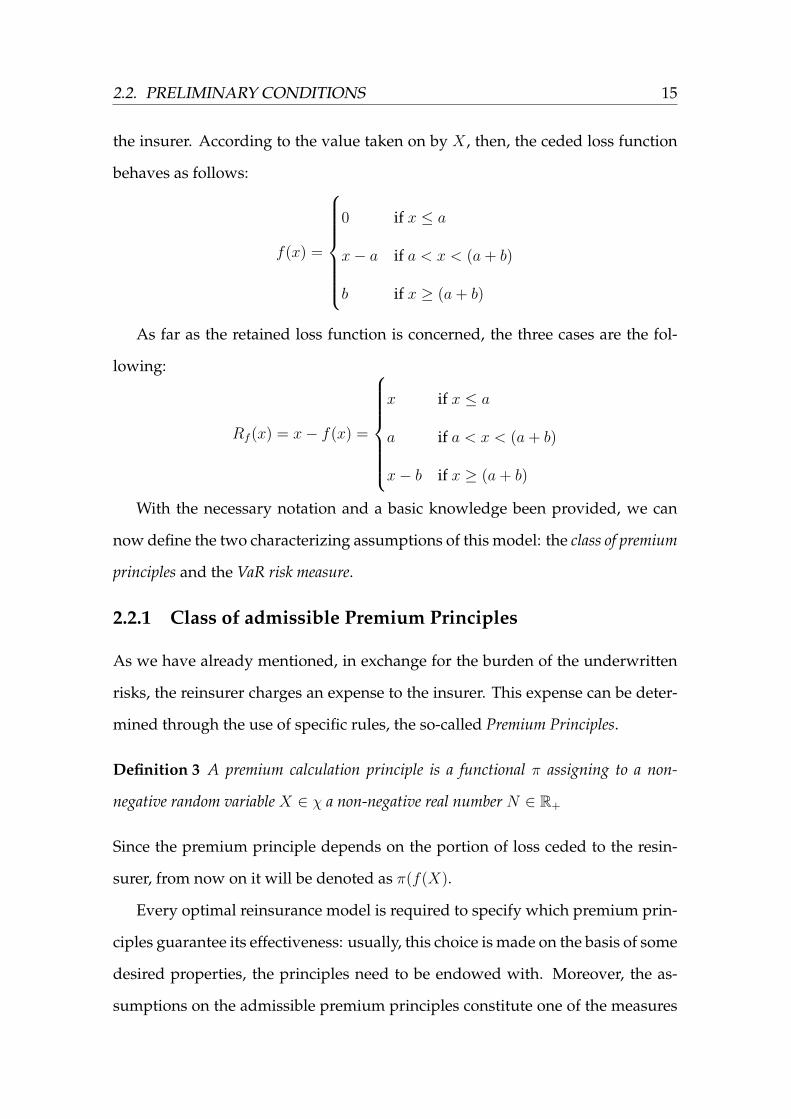
As far as the retained loss function is concerned, the three cases are the fol-

lowing:

Rf (x) = x− f(x) =

x if x ≤ a

a if a < x < (a+ b)

x− b if x ≥ (a+ b)

With the necessary notation and a basic knowledge been provided, we can

now define the two characterizing assumptions of this model: the class of premium

principles and the VaR risk measure.

2.2.1 Class of admissible Premium Principles

As we have already mentioned, in exchange for the burden of the underwritten

risks, the reinsurer charges an expense to the insurer. This expense can be deter-

mined through the use of specific rules, the so-called Premium Principles.

Definition 3 A premium calculation principle is a functional π assigning to a non-

negative random variable X ∈ χ a non-negative real number N ∈ R+

Since the premium principle depends on the portion of loss ceded to the resin-

surer, from now on it will be denoted as π(f(X).

Every optimal reinsurance model is required to specify which premium prin-

ciples guarantee its effectiveness: usually, this choice is made on the basis of some

desired properties, the principles need to be endowed with. Moreover, the as-

sumptions on the admissible premium principles constitute one of the measures


of a model’s robustness: the higher the number of admissible premium prin-

ciples, the more robust the model. This is what led Chi and Tan to relax the

assumption of a premium calculated according to the Expected Value principle

(see [4]). In Chi and Tan (2013), in fact, the model is not constrained to a specific

premium principle, but to a wider set of them. In particular, this set is composed

of every premium principle satisfying these three properties (see [5]):

1. Distribution invariance: For any X ∈ χ, π(X) depends only on the c.d.f.

FX(x).

Also known as independence, the meaning of this property is that the pre-

mium does not depend on the cause of a loss, but only on its monetary

value and on the probability that it occurs.

2. Risk-loading: π(X) ≥ E[X] for all X ∈ χ.

The reinsurer needs to charge not only the expected value of the risk X ,

but also the uncertainty that it entails: otherwise, on average, it will lose

money;

3. Stop-loss ordering preserving: For X, Y ∈ χ, we have π(X) ≤ π(Y ), if X is

smaller than Y in the stop-loss order (denoted as X ≤sl Y ).

Hürlimann (2002) defines the degree n stop-loss transform of a non-negative

random variable X , for each n = 0, 1, 2, ..., as «the collection of partial

moments of order n» given by ΠnX(x) = E[(X − x)n+], with x ∈ R (see

[Hurlimann2002]). An exception is made for the 0th stop-loss transform,

which is conventionally determined as Π0X(x) = SX(x) = 1− FX(x).

The following definitions result:


Definition 4 The random variableX precedes Y in the 0th stop-loss order, written

X ≤st Y , if the moments of order 0 are finite and

Π0X(x) = SX(x) ≤ Π0

Y (x) = SY (x), uniformly for all x ∈ R.

Definition 5 The random variableX precedes Y in the 1st stop-loss order, written

X ≤sl Y , if the moments of order 1 are finite and

ΠX(x) = E[(X − x)+] ≤ ΠY (x) = E[(Y − x)+], uniformly for all x ∈ R.

It is possible to identify at least 8 premium principles, among the most com-

mon ones, that satisfy the above axioms: this corroborates the model, proving

its robustness. For the purpose of this thesis, we can confine the analysis of the

individual premium principles to their statements (see [25]).

1. Net Premium Principle: π(X) = E[X];

2. Expected Value Premium Principle: π(X) = (1 + θ)E[X], for some θ > 0;

3. Exponential Premium Principle: π(X) = (1/α) · lnE[eαX ], for some α > 0;

4. Proportional Hazards Premium Principle: π(X) =∫∞0

[SX(t)]c dt, for some

0 < c < 1;

5. Principle of Equivalent Utility: π(X) solves the equation

u(w) = E[u(w −X + π(X))],

where u is an increasing, concave utility of wealth andw in the initial wealth;

6. Wang’s Premium Principle: π(X) =∫ c0g[SX(t)] dt, where g is an increasing,

concave function that maps [0,1] onto [0,1];

7. Swiss Premium Principle: π(X) solves the equation

E[u(X − pH)] = u((1− p)H),

for some p ∈ [0, 1] and some increasing, convex function u;


8. Dutch Premium Principle: π(X) = E[X] + θE[(X−αE[x])+], with α ≥ 1 and

0 < θ ≤ 1.

All the principles above can be used by insurers, as well as reinsurers: in the first

case, the premium is computed on X ; in the second, on f(X).

Besides the premium principle, the other characterizing assumption of an op-

timal reinsurance model concerns the risk measure. This model was studied un-

der both the VaR and the CVaR risk measure, but we have chosen to focus only

on the Value-at-Risk.

2.2.2 VaR Risk Measure

The Value-at-Risk, from now on denoted as VaR, is a common risk measure among

both the banking and insurance sectors and it plays a major role in their regula-

tions, as far as the capital requirements are concerned.

Before entering into a deeper analysis of its meaning and properties, it is use-

ful to introduce its definition. Chi and Tan (2013) propose the following:

Definition 6 The VaR of a non-negative random variable X at a confidence level 1− α

where 0 < α < 1 is defined as

V aRα(X) , infx ≥ 0 : P (X > x) ≤ α

In simple words, it is the (1-α)-quantile of the random variable X and it indicates

how much, at most, it is possible to lose at the confidence level 1 − α. Being

expressed in units of lost money, its interpretation is immediate.

Denuit et al (2004) finds worth noticing that V aRα(X) = F−1X (1 − α), where

F−1X (p) is the inverse of the cumulative density function of the random variable

X , with 0 < p < 1 (see [8]). Considering definition in (2.1), the above states that

the value (a real number) taken on by X with probability p = 1 − α is exactly

V aRα(X); also, it implies that the probability of X taking on a value smaller than

V aRα(X) is p = 1 − α. Equivalently, V aRα(X) = S−1X (α), where S−1X (p) with


0 < p < 1 is the inverse of the survival function. According to the definition

in (2.2), this statement emphasizes that the probability of X taking on a value

greater than V aRα(X) is p = α. It is clear that V aRα(X) = 0 when α ≥ SX(0):

therefore, we assume 0 < α < SX(0).

In light of the above, it emerges that α is to be intended as the level of risk ac-

cepted by the insurer. Moreover, we can deduce that the VaR is endowed with all

the intrinsic properties of a quantile function: in particular, it is an increasing, left-

continuous function. As a consequence, the property demonstrated by Dhaene

et al (2002) holds (see Theorem 1, [9]), and

V aRα(g(X)) = g(V aRα(X)) (2.7)

is true for any increasing and left-continuous function g. Moreover:

1. For any constant c,

V aRα(X + c) = V aRα(X) + c;

2. For any comonotonic random variables X and Y ,

V aRα(X + Y ) = V aRα(X) + V aRα(Y ),

where the concept of comonotonicity can be explained through the sequence

of definitions that follows (see Dhaene et al (2002), [9]).

Definition 7 A bivariate random vector (X, Y ) is said to be comonotonic if it has

a comonotonic support.

Definition 8 Any subset A ⊆ R × R is called support of (X, Y ), if P ((X, Y ) ∈

A) = 1 holds true.

Definition 9 The set A ⊆ R × R is said to be comonotonic, if each two bivariate

random vectors in A are ordered componentwise.


3. For any random variables X ≤ Y ,

V aRα(X) ≤ V aRα(Y ).

It is important to underline that the VaR does not satisfy the property of sub-

additivity, meaning that V aRα(X +Y ) ≤ V aRα(X) +V aRα(Y ) is not always true.

This entails the most argued downside of this risk measure: it is not a coherent

risk measure. A coherent risk measure is usually eligible, since it is translative,

positive homogeneous, subadditive and monotone: in our case, though, the lack

of coherence does not constitute a severe limitation.

With all the assumptions been set and all the fundamental tools been intro-

duced, we can finally proceed with the statement and the solution of the model.

2.3 A VaR minimization model

Initially, the total risk exposure of the insurer is represented by X . Buying rein-

surance, the insurer lowers its exposure by transferring part of its underwritten

risks to the reinsurer; in exchange, it pays a premium. Therefore, considering

the partitioning of X in (2.3) and the premium paid for reinsurance, the total risk

exposure Tf (X) of the cedant is given by:

Tf (X) = Rf (X) + π(f(X))

Consequently, V aRα(Tf (X)) measures the maximum loss reasonably predictable

by the cedant at a confidence level 1− α.

The model is set so as to determine the ceded loss function that minimizes the

VaR of the total exposure of the cedant: in this sense, it is said to be optimal. In

short, the model can be written as

V arα(Tf∗(X)) = minf∈C

V aRα(Tf (X)), (2.8)

2.3. A VAR MINIMIZATION MODEL 21

where Tf∗(X) is the total exposure of the cedant, when the ceded loss function is

optimal (denoted as f ∗). Obviously, since f is assumed to belong to C (defined in

(2.4)), also f ∗ ∈ C.

The solution of the model provided by Chi and Tan (2013) builds on specific

key steps. We think it is useful to first introduce them theoretically and then

proceed with their mathematical demonstration. These are:

1. Firstly, for any ceded loss function f ∈ C,

hf (x) , min(x− (V aRα(X)− f(V arα(X)))

)+, f(V aRα(X))

,

x ≥ 0

(2.9)

is defined. We can see that hf (x) is a layer reinsurance policy of the form

(2.6), having deductible equal to V aRα(X) − f(V arα(X)) and upper limit

equal to f(V aRα(X)). Its peculiarities are:

a) The ceded loss function hf (x) is increasing, and so is the relative re-

tained function Rhf (x). Then:

hf (x) ∈ C.

b) The VaR of the ceded loss function hf (x) is equal to the VaR of any

ceded loss function f(x). Obviously, the same is true for the relative

retained functions. Moreover, exploiting VaR’s property in (2.7):

hf (V aRα(X)) = f(V aRα(X)). (2.10)

c) The total exposure of the insurer, when the ceded loss function is equal

to hf (x), is

Thf (X) = Rhf (X) + π(hf (X))

2. Secondly, this layer reinsurance treaty is proved to be optimal, by showing

that V aRα(Thf (X)) is smaller or equal than V aRα(Tf (X)). The proof relies


on the fact that the VaRs of the two retained functions are equal, while the

premium paid for (2.9) is smaller.

3. Lastly, it is shown that the layer reinsurance (2.6), with b < ∞, is always

optimal. In addition, it is possible to rewrite (2.9) as

hf (x) , min

(x− a)+, (V aRα(X)− a),

= (x− a)+ − (x− V aRα(X))+

(2.11)

and the problem of determining the optimal ceded loss function can be re-

arranged in terms of the optimal deductible a of a limited stop-loss reinsur-

ance.

Finally, the solution of the model is the following (see [5].

Theorem 1 For the VaR-based optimal reinsurance model (2.8), the layer reinsurance of

the form (2.9) is optimal in the sense that

V aRα(Thf (X)) ≤ V aRα(Tf (X)), ∀ f ∈ C (2.12)

Moreover, we have

minf∈C

V aRα(Tf (X)) = minf∈Cv

V aRα(Tf (X))

= min0≤α≤V aRα(X)

a+ π

(min(X − a)+, V aRα(x)− a

),

(2.13)

where

Cv ,min(x− a)+, V aRα(X)− a : 0 ≤ a ≤ V aRα(X)

(2.14)

Proof. First of all, we need to demonstrate that for any f ∈ C

hf (x) ≤ f(x), ∀x ≥ 0 (2.15)

with hf (x) defined in (2.9). We identify two cases.

If 0 < x < V aRα(x), we can use the Lipschitz-continuity property of f in (2.5),

so that

0 ≤ f(V arα(x))− f(x) ≤ V aRα(X)− x, ∀ 0 ≤ x ≤ V aRα(X)

2.3. A VAR MINIMIZATION MODEL 23

Rearranging, we obtain

0 ≤(x+ f(V aRα(X))− V aRα(x)

)+≤ f(x), ∀ 0 ≤ x ≤ V aRα(X) (2.16)

Since f ∈ C is increasing, x < V aRα(x) implies f(x) < f(V aRα(x)). Then

0 ≤(x+ f(V aRα(X))− V aRα(x)

)+≤ f(x) ≤ f(V aRα(X)),

from which it can be deduced that

hf (x) =(x+ f(V arα(X))− V arα(X)

)+

Finally, from (2.16) it is straightforward that

f(x) ≥ hf (x), ∀ 0 ≤ x ≤ V aRα(X)

proving that in this case (2.15) holds.

If x ≥ V aRα(x), we can rely on the increasing property of f to derive:

f(x) ≥ f(V aRα(X))

It is immediate to deduce that f(V aRα(X)) ≤(x + f(V aRα(X)) − V aRα(X)

),

and then

hf (x) = f(V aRα(X))

f(x) ≥ hf (x), ∀x ≥ V aRα(X)

In both cases, and then for any x ≥ 0, equation (2.15) holds and the evalua-

tion of f(x) on x is greater or equal to the evaluation of hf (x). Moreover, from

definitions 4 and 5, we can draw that hf (X) precedes f(X) in both the 0th and

1st stop-loss orders. This result can be written as:

hf (X) ≤st f(X)

hf (X) ≤sl f(X)


Let us now recall one of the properties satisfied by the assumed set of admissible

premium principles: stop-loss ordering preserving. Given the above findings, this

property allows us to state that

π(hf (X)) ≤ π(f(X)), (2.17)

meaning that the premium computed on hf (X) is lower than any other premium

computed on f ∈ C. To determine whether the layer reinsurance treaty hf (x) is

optimal, one last step is required. We know that

V aRα(Tf (X)) = V aRα

(Rf (X) + π(f(X))

).

Thanks to the translation invariance property of VaR, we can rewrite it as

V aRα(Tf (X)) = V aRα(Rf (X)) + π(f(X))

Since Rf (x) is assumed to be increasing and Lipschitz-continuos, we can use the

property of VaR defined in (2.7) to write

V aRα(Tf (X)) = Rf (V aRα(X)) + π(f(X))

and then use the partitioning of X , in (2.3), to rearrange it as

V aRα(Tf (X)) = V aRα(X) + π(f(X))− f(V aRα(X))

But we know that hf (V aRα(X)) = f(V aRα(X)), so that

V aRα(Tf (X)) = V aRα(X) + π(f(X))− hf (V aRα(X))

At this point, it is obvious that the only difference between V aRα(Thf (X)) and

V aRα(Tf (X)) consists in the premium: thanks to (2.17), we can deduce that

V aRα(Thf (X)) ≤ V aRα(Tf (X)), ∀ f ∈ C

proving that the constructed layer reinsurance treaty hf (X) is optimal. Now, we

can set a = V aRα(X)− f(V aRα(X)) ans substitute it into the definition of hf (x).

Clearly, 0 ≤ a ≤ V aRα(X). The set described in (2.14),

Cv ,min(x− a)+, V aRα(X)− a : 0 ≤ a ≤ V aRα(X)

,

2.4. CONCLUSIONS 25

is then composed of all the layer reinsurance policies of the form hf (x). In par-

ticular, every layer reinsurance treaty in Cv is a stop-loss reinsurance treaty with

deductible a and upper limit (V aRα(X)− a). Since Cv ⊆ C, the equation

minf∈C

V aRα(Tf (X)) = minf∈Cv

V aRα(Tf (X))

does not need further explanations. Finally, substituting V aRα(Tf (X)) with its

definition in terms of a, we obtain (2.13). Its meaning is crucial: the minimum

VaR obtainable through the choice of the optimal ceded loss function is equal

to the minimum VaR obtainable through the choice of the optimal deductible

and upper limit of a layer reinsurance. The optimization problem faced by the

insurer results significantly simplified, since it only depends on three parameters:

a, V aRα(X) and π(f(X).

2.4 Conclusions

In this chapter, we studied the solution proposed in Chi and Tan (2013), to a

VaR-based optimal reinsurance model from the perspective of the insurer (see

[5]). The hypothesis were confined to a set of premium principles satisfying three

basic axioms (distribution invariance, risk loading and stop-loss ordering pre-

serving) and to the assumption that both the insurer and the reinsurer need to

pay more for larger losses.

The authors built an ad hoc layer reinsurance treaty, which was characterized

by a VaR equal to the one of any other admissible ceded loss function, but which

entailed a lower premium: it was proved to be optimal. Introducing a new pa-

rameter a, it was possible to generalize the optimal layer reinsurance policy to

the standard form of a limited stop-loss reinsurance: under the specified set of

assumptions, a limited stop-loss reinsurance with deductible a and upper limit

(V aRα(X) − a) is always optimal. In light of these results, it was possible to

simplify the optimal reinsurance problem of the insurer. In fact, to minimize the


VaR of the total exposure of the cedant, it is enough to determine the optimal

deductible and upper limit of a layer reinsurance.

The robustness of the model is upheld by the wider set of admissible rein-

surance premium principles. By choosing a speific premium principle, explicit

solutions of the optimal parameters are derivable: going beyond the purpose of

this thesis, though, this topic will not be discussed.

CHAPTER 3

THE PERSPECTIVE OF THE REINSURER

3.1 Topic of research and existing literature

In reinsurance research, the perspective of the reinsurer, considered singularly,

has not been extensively studied. In our opinion, though, meaningful results

might derive from its unconstrained optimization problem.

Among the studies concerning the reinsurer, it is worth citing Huang and Yu

(2017) (see [14]). The authors assume the insurer to behave rationally, mean-

ing that it chooses the form and level of reinsurance proved optimal, and the

premium to be computed according to the Expected Value principle π(X) =

(1 + θ)E[X], for some θ > 0. The optimal safety loading θ is then studied, with

respect to three different optimality criteria: maximizing the expectation and the

utility of the reinsurer’s profit and minimizing the VaR of its total loss.

In this chapter, we contribute to the existing literature by analyzing the VaR-

based problem of Chi and Tan (2013), from the perspective of the reinsurer: our

aim is to determine the ceded loss function that minimizes the VaR of its total risk

exposure. The assumptions underlying the model are the same. This is novel in

the literature, since a general solution to the unconstrained optimization prob-

lem of the reinsurer, under the VaR criterion, is yet to be determined. Moreover,

our wide class of admissible premium principle would endow the model with

remarkable robustness.

27

28 CHAPTER 3. THE PERSPECTIVE OF THE REINSURER

3.2 The optimization problem of the reinsurer

We denote the total risk exposure of the reinsurer as TRf (X) and we define it as

TRf (X) = f(X)− π(f(X)), (3.1)

where f(X) is the portion of loss ceded to the reinsurer and π(f(X)) is the pre-

mium paid by the insurer. It is immediate how the reinsurer’s exposure is re-

versed, with respect to the insurer’s one. In this case, the total exposure increases

with the ceded loss function: it is obvious, since the greater the portion of loss

ceded by the insurer, the higher the risk borne by the reinsurer. The premium, on

the other hand, constitutes a cash inflow: this is why it lowers the total exposure

of the undertaker.

In our model, we are interested in assessing whether it is possible to deter-

mine a general form of reinsurance, which minimizes the VaR of the total risk

exposure of the reinsurer. The model can then be summarized as

V aRβ(TRf∗(X)) = minf∈C

V aRβ(TRf (X)), (3.2)

where β is the level of risk accepted by the reinsurer and C is the set defined in

(2.4). It is reasonable to assume β 6= α, since reinsurance companies can afford

better risk management strategies and can be expected to tolerate a higher level

of risk. Furthermore, we assume 0 < β < Sx(0) and all the assumptions discussed

in section (2.2) continue to apply.

As first question of research, we wonder whether the optimal solution derived

for the insurer could be a solution also to the reinsurer’s problem. The question

is answered in the following subsection.

3.2.1 Different solutions for the two agents

In section (2.3), we proved that the optimal ceded loss function for the insurer,

under our set of assumptions, has the form of a limited stop-loss reinsurance. In

3.2. THE OPTIMIZATION PROBLEM OF THE REINSURER 29

particular, a key step in the proof was the construction of hf (X): thanks to some

of its peculiar properties, its optimality was first proven and then generalized.

Below, we recall its definition (first proposed in (2.9)):

hf (X) , min(x− (V aRα(X)− f(V aRα(X)))

)+, f(V aRα(X))

, x ≥ 0

When the point of view of the reinsurer is considered, an adjustment of the

above is required. In the derivation of the optimal form of reinsurance for the

insurer, we considered its level of risk α. The level of risk of the reinsurer, though,

is different: in particular, it is assumed to be equal to β. When trying to determine

whether this form of reinsurance may be optimal for the reinsurer, too, it makes

sense to take into account its own level of risk. Thus, we define hβ,f (x) as

hβ,f (x) , min(x− (V aRβ(X)− f(V aRβ(X)))

)+, f(V aRβ(X))

,

x ≥ 0

(3.3)

Ideally, it is simply the optimal solution we would have derived in section (2.3),

if we had assumed the level of risk of the insurer to be defined by β. Since the

provided proof only required 0 < α < SX(0), as long as β is included in the same

interval, our results hold. Of course, all the properties of hf (x) are valid also for

hβ,f (x).1

By exploiting some of these properties, it is possible to prove that, as far as the

reinsurer is concerned, hβ,f (x) is not optimal: under the VaR criterion, the optimal

form of ceded loss function for the cedent is not optimal for the cessionary. So,

our statement is

V aRβ(TRhβ,f (X)) 6= minf∈C

V aRβ(TRf (X)), (3.4)

which can be proven by showing that

V aRβ(TRf (X)) < V aRβ(TRhβ,f (X)) (3.5)

1For the details, see page 21.


The proof follows. Given the above definition of total exposure of the reinsurer,

V aRβ(TRf (X)) = V aRβ

(f(X) + (−π(f(X)))

)= V aRβ(f(X)) + (−π(f(X)))

= f(V aRβ(X)

)− π(f(X)),

where the second inequality relies on the translation invariance of the VaR, whereas

the third uses the increasing and Lipschitz-continuity property of f ∈ C. Further,

knowing that f(V aRβ(X)) = hβ,f (V aRβ(X)),

V aRβ(TRf (X)) = hβ,f(V aRβ(X)

)− π(f(X))

Finally, we can use π(f(X)) ≥ π(hβ,f (X)), to determine:

V aRβ(TRf (X)) ≤ hβ,f(V aRβ(X)

)− π(hβ,f (X))

≤ V aRβ(TRhβ,f (X))

At this point, to prove that hβ,f (X) is not optimal, it is necessary to show that

the strict inequality in (3.5) holds true, at least in one case. Mathematically, a

similar proof would require more stringent assumptions. Conceptually, though,

a similar conclusion is reasonable: in fact, when the strict inequality

π(hβ,f (X)) < π(f(X)) (3.6)

is true, also (3.5) is valid.

This result is trivial. If both the cedent and the cessionary’ decisions are taken

upon the same criterion, i.e. minimizing a chosen risk measure on their total

exposures, a conflict of interests arises. The cedent would rather transfer a greater

portion of loss, paying the lowest premium possible. The cessionary, on the other

hand, would rather bear a lower risk, being paid as high as possible. Because of

this, hβ,f (X) could not have been optimal for the reinsurer. As explained earlier,

the peculiarities of this ceded loss function perfectly fit the interests of the insurer:

it guarantees a Value-at-Risk of the retained loss function equal to the one of any


other admissible, but it allows for a lower premium to be paid. Obviously, this

same peculiarities make it not eligible for the reinsurer.

3.2.2 An optimal solution for the reinsurer

In this section, we try to solve the Var-based optimal reinsurance model in (3.4).

Our purpose is to derive a general form of optimal ceded loss function, which

minimizes the total exposure of the reinsurer under our set of assumptions. To

do so, we resort to a simple intuitive reasoning, starting from the results obtained

for the insurer.

In theorem 1, a solution to the VaR-based optimal reinsurance model defined

in (2.8) was obtained. Our findings can be summarized as2

minf∈C

V aRα(T If (X)) = V aRα(T Ihf (X))

As explained before, a change in the assumed level of risk does not compromise

our results. Hence, considering our aim of deriving further insights from the

point of view of the reinsurer, we substitute the level of risk of the insurer, α,

with the reinsurer’s one, β.

minf∈C

V aRβ(T If (X)) = V aRβ(T Ihβ,f (X)) (3.7)

The meaning is simple: when the ceded loss function takes the form of the layer

reinsurance hβ,f (x), the Value-at-Risk of the total exposure of the cedent is mini-

mized. Using the definition of T Ihβ,f (X), we can write:

V aRIβ(T Ihβ,f (X)) = V aRI

β

(X − hβ,f (X) + π(hβ,f (X))

)(3.8)

Let us recall thatX−hβ,f (X) represents the retained function of the insurer, while

the premium π(hβ,f (X) depends on the ceded loss function hβ,f (X). Further,

since hβ,f (X) is a layer reinsurance, it can be rewritten according to (2.6) as

hβ,f (X) =(x− V aRβ(X) + f(V aRβ(X))+ − (x− V aRβ(X))+

)2To avoid misunderstandings, from now on the superscript I will be used to identify the

perspective of the insurer: i.e. T If (X) will denote the total exposure of the cedent.


Then, for any value x ≥ 0 taken on by the random variable X , equation (3.8) is

V aRβ(T Ihβ,f (x)) =V aRβ

(x−

(x− V aRβ(X) + f(V aRβ(X))

)+

+

+(x− V aRβ(X)

)+

+ π(hβ,f (X))) (3.9)

Now, let us assume full transparency between the insurer and the reinsurer: in

particular, the latter is informed not only of f(X), but also of the original X as-

sumed by the insurer. This allows us to introduce a function lf (x), such that

lf (x) , x−(x− V aRβ(X) + f(V aRβ(X))

)+

+(x− V aRβ(X)

)+

= x−min(x− (V aRβ(X)− f(V aRβ(X)))

)+, f(V aRβ(X))

= x− hβ,f (x)

(3.10)

Since hβ,f (x) ∈ C, it is straightforward that also lf (x) ∈ C, making it an admissible

ceded loss function under our set of assumptions. When the ceded loss function

is lf (x), the VaR of the total exposure of the reinsurer, for any x ≥ 0, is

V aRβ(TRlf (x)) =V aRβ

(x−


)+

+

+(x− V aRβ(X)

)+− π(lf (X))

) (3.11)

Let us compare equations (3.9) and (3.11). In equation (3.9), the first part of the

argument,(x−


)+

+(x− V aRβ(X)

)+

),

represents the retained loss function Rhβ,f (x), or rather the portion of loss borne

by the cedent; the same, in equation (3.11), represents the ceded loss function

lf (x), or rather the burden of risk of the cessionary. Despite the conceptual dif-

ference among the two, they are mathematically identical. What changes, on the

other hand, is the premium. Being dependent on the ceded loss function, in the

total exposure of the insurer it is computed according to hβ,f (x); in the total ex-

posure of the reinsurer, instead, it is computed according to lf (x) = x − hβ,f (x).

Furthermore, since the premium has opposite impacts on the exposures of the

agents, in equation (3.11) it is of opposite sign.


In light of these hints, it is noticeable that lf (x) = Rhβ,f (x), for any x ≥ 0. It

follows that

lf (V aRβ(X)) = Rhβ,f (V aRβ(X)) (3.12)

We can now use one of the properties hβ,f was endowed with, by construction:

V aRβ(hβ,f (X)) = V aRβ(f(X)). Since hβ,f (x), f(x) ∈ C, both the functions are

increasing and continuous. We are then allowed to use a property of the VaR,

defined in (2.7), to derive f(V aRβ(X)) = hβ,f (V aRβ(X)). Straightforwardly, also

V aRβ(X)− f(V aRβ(X)) = V aRβ(X)− hβ,f (V aRβ(X))

is true. Recalling the definition of the retained loss function, this can be rewritten

as

Rhβ,f (V aRβ(X)) = Rf (V aRβ(X)), (3.13)

which leads to

lf (V aRβ(X)) = Rf (V aRβ(X)), (3.14)

thanks to the transitive property of equality. Now, under the same assumptions

used to introduce lf (x), let us introduce a ceded loss function gf (x), such that

gf (x) , x− f(x)

Since f(x) ∈ C, then also gf (x) is included in our set of admissible ceded loss

functions. Moreover, basing on the reasoning leading to lf (x) = Rhβ,f (x), we can

draw that gf (x) = Rf (x), for any x ≥ 0. Then, gf (V aRβ(X)) = Rf (V aRβ(X)) and

equation (3.14) becomes:

lf (V aRβ(X)) = gf (V aRβ(X)) (3.15)

In the previous chapter, in the proof of theorem 1, we demonstrated that

hf (x) ≤ f(x), for any x ≥ 0. The result holds up for any 0 < α < SX(0), so

hβ,f (x) ≤ f(x)


is also true. A direct consequence is that, for any x ≥ 0,

lf (x) = x− hβ,f (x)

≥ x− f(x)

≥ g(x)

Basing on the same proof, we use definition 5 to infer that gf (x) precedes lf (x) in

the 1st stop-loss order, written

gf (X) ≤sl hf (X)

Following through, since all the admissible premium principles are assumed to

satisfy the stop-loss ordering preserving property, we can conclude that

π(gf (X)) ≤ π(lf (X)) (3.16)

What we found, is that a ceded loss function of the form of lf (X) consents the

reinsurer to collect a higher premium. This result is of particular significance.

The premium is in inverse proportion to the total exposure of the reinsurer: a

ceded loss function allowing for a higher premium, and all else being equal, can

then be expected to lead to a lower total exposure of the reinsurer.

Given the results summarized in equations (3.14) and (3.16), we can write

lf (V aRβ(X))− π(lf (X)) ≤ gf (V aRβ(X))− π(gf (X)),

which is equal to

V aRβ(lf (X))− π(lf (X)) ≤ V aRβ(gf (X))− π(gf (X)),

provided that both lf (x) and gf (x) are increasing and continuous functions. Then,

thanks to the translation invariance of the VaR, we can rewrite the above as

V aRβ

(lf (X)− π(lf (X))

)≤ V aRβ

(gf (X)− π(gf (X))

)Therefore, according to the definition of TRf (X),

V aRβ(TRlf (X)) ≤ V aRβ(TRgf (X)), (3.17)


which proves that a ceded loss function of the form of lf (x) allows the reinsurer

for a total exposure always equal or lower than the one obtainable with a generic

gf (x) = x− f(x). Then

ming∈C

V aRβ(TRgf (X)) = V aRβ(TRlf (X)) (3.18)

But can this result be generalized to any function f ∈ C?

Let us consider our set of admissible ceded loss function C: it is composed of

all the increasing f(x), such that the retained loss functionRf (x) = x−f(x) exists

and it is increasing. Noticing that I(x) = x is the identity function, which assigns

every real number x to the same real number x, we can write Rf (x) as

Rf (x) = I(x)− f(x)

and f(x) as

f(x) = I(x)−Rf (x)

Within C, then, f(x) can always be expressed as the identity function minus a

generic increasing function Rf (x). Moreover, Rf (x) belongs to C. It follows that,

under the perspective of the insurer, if

minf∈C

V aRβ(T If (X)) = V aRβ(T Ihβ,f (X)),

then

V aRβ(T Ihβ,f (X)) ≤ V aRβ(T II(x)−f(x)(X))

is also true. But, by construction,

I(x)− gf (x) = I(x)− I(x) + f(x)

= f(x)

and so, from (3.18), it is possible to deduce that

V aRβ(TRlf (X)) ≤ V aRβ(TRf (X)) (3.19)


Thus, we have proved that

minf∈C

V aRβ(TRf (X)) = V aRβ(TRlf (X)) :

the optimal ceded loss function for the reinsurer, among all the functions in-

cluded in C, has the form of lf (x), defined as

lf (x) , x−(x− V aRβ(X) + f(V aRβ(X))

)+

+(x− V aRβ(X)

)+

To conclude, we set aβ = V aRβ(X) − f(V aRβ(X)) and we substitute it in lf (x).

Doing so, we can rewrite the optimal form of ceded loss function, as

lf (x) = x−min(x− (V aRβ(X)− f(V aRβ(X)))

)+, f(V aRβ(X))

= x−min(x− aβ)+, V aRβ(X)− aβ

= x− (x− aβ)+ + (x− V aRβ(X))+

(3.20)

3.3 A comparative analysis of the results

In sections (2.3) and (3.2.2), we proposed two optimal-reinsurance models from

the perspectives of the insurer and of the reinsurer, respectively. The point of

view of the insurer boasts a wide dedicated literature: the vast diversity of op-

timality criteria have allowed researchers to develop numerous models. Among

the many, we chose a VaR-minimization model, as proposed by Chi and Tan

(2013, see [5]): after an introduction of all the necessary assumptions and through

every step of the mathematical demonstration, the main findings were derived.

Under the perspective of the insurer, the ceded loss function minimizing the

Value-at-Risk of its total risk exposure has the form of a layer reinsurance treaty,

with deductible 0 ≤ a ≤ V aRα(X) and upper bound V aRα(X)− a:

hf (x) = min

(x− a)+, V aRα(X)− a

= (x− a)+ − (x− V aRα(X))+

This layer reinsurance is known as the limited stop loss reinsurance. Under this

contract, the behaviors of the ceded and retained loss functions depend on the

3.3. A COMPARATIVE ANALYSIS OF THE RESULTS 37

value x, taken on by X . In particular, it is possible to identify three ranges, on the

basis of the agreed deductible and upper limit.

hf (x) =

0 if x ≤ a

x− a if a < x < V aRα(X)

V aRα(X)− a if x ≥ V aRα(X)

Rhf (x) =

x if x ≤ a

a if a < x < V aRα(X)

x− (V aRα(X)− a) if x ≥ V aRα(X)

It follows a textual explanation of the behavior of both the ceded and retained

loss function, in each of the three cases above.

1. When x ≤ a, the loss is smaller than the deductible a: the insurer bears the

whole loss and nothing is covered by the reinsurer;

2. When a < x < V aRα(X), the loss is greater than the deductible. The in-

surer bears an amount of loss equal to a and it cedes to the reinsurer the

exceeding part, given by x − a. The presence of an upper bound implies

that the reinsurer agrees on covering a portion of the loss, only as long as

this portion is smaller than a fixed cap, V aRα(X) − a: this limit is reached

when

x− a = V aRα(X)− a

x = V aRα(X)

3. When x ≥ V aRα(X), the reinsurer limits its coverage to a maximum amount,

equal to V aRα(X) − a. The insurer is required to pay for what exceeds it,

that is x− (V aRα(X)− a).

The two functions are graphed in figure (3.1a) and (3.1b).


Then, we shifted to the agent on the other side of the contract: the reinsurer.

Keeping our set of assumptions constant, we introduced an optimal-reinsurance

model aimed at determining the ceded loss function, which minimizes the Value-

at-Risk of the reinsurer’s total risk exposure.

First, we proved that the form of reinsurance, which is optimal for one party,

is not optimal for the other: this was expected. When both of the agents want to

minimize their maximum potential loss, their antithetical positions cannot avoid

leading to a conflict of interests: each party would rather the other to bear the

most of the loss. This conflict is only partially mitigated by the premium: a rein-

surer might be willing to accept the transfer of a greater portion of the loss, if this

allows it to gain in terms of the receivable premium. Obviously, the opposite is

true for the insurer.

Secondly, we derived a general form of the ceded loss function, which is

proved optimal for the reinsurer:

lf (x) = x−min(x− aβ)+, V aRβ(X)− aβ

= x− (x− aβ)+ + (x− V aRβ(X))+

The most important implication of this result is that

lf (x) = x− hβ,f (x),

where hβ,f is the optimal ceded loss function of an insurer, which accepts a level

of risk equal to the reinsurer. Also in this case, it is possible to study the behavior

of lf (x), on the basis of the value x.

lf (x) =

x if x ≤ a

a if a < x < V aRβ(X)

x− (V aRβ(X)− a) if x ≥ V aRβ(X)

3.4. CONCLUSIONS 39

It is straightforward that when α = β, meaning that the levels of risk of the

insurer and of the reinsurer are equal,

lf (x) = Rhf (x) ∀x > 0

In simple words, lf (x) describes the portion of loss that, if borne by either of

the agents, allows it to minimize the VaR of its total risk exposure. Therefore,

the graphical representation of lf (x) is the one in figure (3.1b): it shows that the

reinsurer is willing to cover the whole loss, as long as this is smaller than an

agreed level a; when the loss is bigger than a, moved by the aim of protecting

itself, it is disposed to cover only a fixed amount, that is a; when the loss exceeds

V aRα(X), it agrees on covering x− (V aRα(X)− a). Practically, he would rather

be on the other side of the contract.

When β 6= α, the difference between the levels of risk of the two agents leads

to an asymmetry: the optimal solutions of the agents are not exactly reversed. If

the reinsurer is willing to tolerate a higher level of risk, β ≥ α, it is more likely to

be disposed of covering a greater portion of loss, lowering the threshold, up to

which it only pays for a fixed amount a. Anyway, though, a difference between

α and β as big as to allow for an agreement, is hardly imaginable in practice.

3.4 Conclusions

In this chapter, we proved that when both the insurer and the reinsurer aim at

minimizing the VaR of their total exposures, they are unlikely to conclude a con-

tract. In fact, the optimal solution of one party would lead to an unacceptable

high value of the other’s VaR. Moreover, in the extreme scenario, in which the

level of risk is the same for both agents, the solutions to their unconstrained opti-

mization problems are exactly hf (x) and x−hf (x): in simple words, the reinsurer

would need to be transferred the exact portion of loss, that the insurer would

need to retain.


From these results, it arises the necessity of a third reinsurance model, capa-

ble of taking into account the opposite interests of the parties, in the attempt of

determining an optimal halfway solution. In the literature, two main models of

this kind have been proposed: these are studied in the next chapter.

3.4. CONCLUSIONS 41

(a) Optimal ceded loss function of the insurer

(b) Retained loss function of the insurer,when the ceded loss function is optimal

Figure 3.1: Graphical representation of hf (X) and Rhf (X)

CHAPTER 4

THE PERSPECTIVE OF BOTH

4.1 Multi-objective Optimization

So far, we have studied the individual perspectives of the two agents involved

in a reinsurance contract. For each, a VaR-based optimal reinsurance model has

been analyzed and solved: what emerged, is that the solutions of the respective

unconstrained optimization problems are incompatible.

As a consequence, the necessity of a third optimization problem arises: its pe-

culiarity is the presence of two objective functions, which need to be optimized

simultaneously. In economics, this problem is endowed with a clear interpreta-

tion: indeed, it theorizes the attempt of the reinsurer to design a contract which

satisfies its optimality requirements, being at the same time attractive for the in-

surer. In mathematics, it is a Two-objective Optimization Problem.

Multi-objective Optimization is an area of research, which allows to formalize

and solve optimization problems with two or more optimality criteria. Miettinen

(1998, see [22]) describes the general form of a multicriteria optimization problem

as

minx∈S

(f1(x), f2(x), ..., fk(x))T (4.1)

Given each objective function fi(x) : Rn → R, for i = 1, 2, ..., k and k > 1,

• f(x) = (f1(x), f2(x), ..., fk(x))T is the vector of objective functions,

43

44 CHAPTER 4. THE PERSPECTIVE OF BOTH

• x = (x1, x2, ..., xn)T is the decision variable vector,

• z = (z1, z2, ..., zk)T is the objective vector.

S is the set of constraints defining the feasible region, to which the variable vectors

belong: obviously S ⊆ Rn, with the latter being the decision variables space. Z =

f(S) is the feasible objective region, computed as the image of the feasible region: it

is defined as

Z = z ∈ Rk : z = f(x), x ∈ S

and it is a subset of the objective space Rk. Every objective vector z ∈ Z is admissi-

ble.

The need for alternative solving methods arises when the ideal vector zid, with

components

zidi = minx∈S

fi(x), with 1 ≤ i ≤ k (4.2)

does not belong to the feasible objective region. Otherwise, (4.2) would be a

banal solution to problem (4.1), easily determinable through the resolution of

k single-objective optimization problems, one for each objective function. As-

suming zid /∈ Z is the same as saying that the objective functions are at least

partly conflicting: in this sense, the resulting Multi-objective Optimization Prob-

lem (MOP) is nontrivial. In this case, a single solution that optimizes all the ob-

jective functions simultaneously does not exist: there exist, though, a number of

Pareto optimal solutions. Thus, we can say that the main aim of Multi-objective

Optimization is to seek Pareto optimal solutions.

Definition 10 A decision variables vector x∗ ∈ S is Pareto optimal, or efficient, if

@x ∈ S, s.t:

fi(x) ≤ fi(x∗) ∀i, i = 1, 2, ...k

fj(x) < fj(x∗) for at least one index j

4.1. MULTI-OBJECTIVE OPTIMIZATION 45

According to the above, a decision variable vector is said Pareto optimal, when it

is impossible to further minimize at least one of the objective functions, without

degrading any of the other objective values. On the same conditions is founded

the definition of Pareto optimal objective vector.

Definition 11 An objective vector z∗ ∈ Z is Pareto optimal, or efficient, if @ z ∈ Z,

s.t:

zi ≤ z∗i ∀i, i = 1, 2, ...k

zj < z∗j for at least one index j

or if the decision variables vector corresponding to z∗ is Pareto optimal.

Usually, the Pareto optimal solution of a MOP is not unique: SE denotes the

efficient set, composed of all efficient solutions x∗ ∈ S; ZN is called nondominated

set or efficient frontier and it includes all the equilibria points, each representing a

nondominated vector z∗ = f(x∗) ∈ Z (see [26, 19]).

Considering the existence of multiple optimal solutions, the goal of a MOP

is not always straightforward. Sometimes, solving a MOP means to derive the

whole efficient set and corresponding efficient frontier; others, it implies the

choice of a single optimal solution, among the many. The latter requires the pres-

ence of a better informed Decision Maker (DM), who can make the selection ac-

cording to its subjective preferences. On the basis of the role played by the DM,

it is possible to distinguish four main categories of Multi-objective Optimization

methods:

1. No-preference methods: in the absence of a DM, a compromise solution is

determined;

2. A priori methods: in light of the DM’s preferences, the solution which best

satisfies them is chosen;


3. A posteriori methods: in light of the set of Pareto optimal solutions, the DM

chooses the one which better satisfies its preferences.

4. Interactive methods: the DM chooses the best solution through an iterative

procedure, by describing how the Pareto optimal solution derived at each

round can be improved.

The above is just one of the many classification criteria used in the literature: i.e.

Kaucic and Daris (2015), referring to Schukla and Deb (2017), identify two major

categories (see [18, 23]). They define as classical the methods resorting to direct

or gradient-based procedures, on the basis of specific mathematical principles;

non-classical are, instead, the ones following natural or physical principles.

In view of what just stated about Multi-objective Optimization, it is clear why

it well-fits our purpose. The objective functions of the insurer and of the reinsurer

have been proven to be conflicting: a unique optimal solution, which simultane-

ously optimizes both of them, does not exist. Through the formalization and

resolution of a MOP, though, we can investigate the existence of a Pareto optimal

solution.

Our Two-objective Optimization problem is formalized as

minf∈C

(V aRα(T If (X)), V aRβ(TRf (X))

)T (4.3)

The two objective functions are the Values-at-Risk of the total risk exposures of

the insurer and of the reinsurer. Their levels of risk are 0 < α < SX(0) and

0 < β < SX(0), respectively. The set C defines our feasible region: 0 ≤ f(X) ≤ X

and both f(x) and Rf (x) are increasing.

As already mentioned, several are the approaches usable to determine a so-

lution: the most commonly used are the weighted sum method and the ε-constraint

methods. Both of them are classical, a posteriori methods. In the following sec-

tions, we explain how these were used in the optimal reinsurance models pro-

posed in Cai, Lemieuz and Liu (2015) and Lo (2017).


4.1.1 Cai, Lemieux and Liu (2015): the weighted-sum method

In Cai, Lemieux and Liu (2015), the optimal reinsurance contract under the per-

spectives of an insurer and a reinsurer is studied (see [3]). Under the assumption

that both of the agents aim at minimizing the VaR of their losses and under the

same set of feasible ceded loss functions C, the solution to each agent’s individual

problem is first derived. The optimal reinsurance contract for the insurer is

f ∗i (x) = (x− V aR 11+θ

(X))+ − (x− V aRα(X))+,

whereas for the reinsurer it is

f ∗r (x) = x− (x− V aR 11+θ

(X))+ − (x− V aRα(X))+

Easily, it is possible to trace back the above to the general optimal forms of ceded

loss functions, derived in the previous chapters and defined in (2.11) and (3.20),

respectively. In addition, the choice of a premium computed according to the

Expected Value premium principle,

π(f(x)) = (1 + θ)E[f(X)],

makes it possible for the authors to specify the optimal levels of deductible a and

upper limit b. Specifically,

a = aβ = V aR 11+θ

(X)

is the optimal deductible for both the insurer and the reinsurer, while the optimal

upper limits are

b =

V aRα(X)− V aR 1

1+θ(X), for the insurer

V aRβ(X)− V aR 11+θ

(X), for the reinsurer

It can be deduced that the different levels of risk, α and β, only affect the upper

limits. The deductible, instead, is a function of the safety loading θ, only.


Given the contradiction of the optimal individual solutions, the authors ad-

dress the problem of determining a reinsurance contract, which simultaneously

takes into account the insurer’s objectives and the reinsurer’s goals. To do so,

they design a Single-objective Optimization Problem, with objective function equal

to the convex combination of the VaR risk measures of the insurer’s loss and the

reinsurer’s loss. Thus,

V (f) = λV aRα

(X − f(X) + π(f(X))

)+ (1− λ)V aRβ

(f(X)− π(f(X)

)is the objective function, with λ ∈ [0, 1]. Despite not explicitly stated, it is possible

to notice that this is the first step of resolution of a Two-objective Optimization

problem, when resorting to the weighted sum method. This method allows to re-

formulate a Multi-objective to a Single-objective Optimization Problem thanks to

a scalarization technique, which is applied by associating each objective function

with a weighting coefficient. The resulting weighted sum is the single-objective

function of the Single-objective Optimization Problem, also called scalar opti-

mization problem or weighted sum scalarization (see [10]). Given a general MOP,

as the one described in (4.1), the scalar optimization problem is formalized as

minx∈S

k∑i=1

λifi(x),

with i = 1, 2, ..., k and k > 1. Each weighting coefficient λi is a real number, such

that λi ≥ 0 and∑k

i=1 λi = 1: the latter means that the weights are normalized.

Then,

minf∈F

V (f), (4.4)

is exactly the weighted sum scalarization of the Two-objective Optimization Prob-

lem

minf∈F

(V aRα

(X − f(X) + π(f(X))

), V aRβ

(f(X)− π(f(X)

))T


This is the model studied in Cai, Lemieux and Liu (2015). The feasible region F

is defined as

F , f ∈ C : f(V aRβ(X))−L2 ≤ π(f(X)) ≤ f(V arα(X))−V aRα(X)+L1, (4.5)

where L1 and L2 are the upper bounds of the VaR risk measures of the insurer

ans reinsurer’ losses, respectively. In fact, the authors assume

V aRα

(X − f(X) + π(f(X))

)≤ L1 (4.6)

and

V aRβ

(f(X)− π(f(X))

)≤ L2, (4.7)

meaning that both agents are willing to reduce the VaR of their total exposure to

a tolerated value, such that

L1 ≤ V aRα(X), with L1 > 0

and

L2 ≤ V aRβ(X), with L2 > 0

Given these constraints, the set F is easily derived in a few steps. Considering

that X and f(X) are comonotonic random variables and thanks to the the trans-

lation invariance of the VaR, as well as to its property defined in (2.7), inequalities

(4.6) and (4.7) can be rewritten as

V aRα(X)− f(V aRα(X)) + π(f(X)) ≤ L1

f(V aRβ(X))− π(f(X)) ≤ L2

Then,

π(f(X)) ≤ f(V aRα(X))− V aRα(X) + L1 (4.8)

f(V aRβ(X))− L2 ≤ π(f(X)) (4.9)


are also true. Since π(f(X)) is equal in both equations, constraints (4.8) and (4.9)

define the set of reinsurance contracts acceptable by both agents, namely F . Fur-

thermore, a premium computed according to the Expected Value premium prin-

ciple continues to be assumed.

At this point, the Pareto optimal solutions are sought by the authors. The

weighted sum method uses a one-at-a-time strategy to generate the entire non-

dominated set. This means that an optimal solution to the problem needs to be

derived, for each value taken on by the weight λ. The authors carry out this

analysis through the study of the following cases:

1. If λ = 0, or if α = β and 0 ≤ λ < 12, problem (4.4) is reduced to

minf∈F

V aRβ

(f(X)− π(f(X))

)2. If λ = 1, or if α = β and 1

2< λ ≤ 1, problem (4.4) is reduced to

minf∈F

V aRβ

(X − f(X) + π(f(X))

)3. If α = β and λ = 1

2

4. If α < β and 0 < λ ≤ 12

5. If α < β and 12≤ λ < 1

6. If α > β and 0 < λ ≤ 12

7. If α > β and 12≤ λ < 1

Besides the trivial solutions of the first two cases, the authors manage to find the

optimal reinsurance contract for each of the cases from 4 to 7: for the details, we

refer to [3, pp. 825-826]. Moreover, each of these solutions is optimal also under

the assumptions in case 3.


The structure of the analysis described above allows for a deeper significance

of the obtained results: it enables a full understanding of how the optimal rein-

surance contract changes, according to how much importance is put by the rein-

surer on having a competitive contract. In cases 5 and 7, in fact, a greater weight

is assigned to the insurer’s optimality criterion; in cases 4 and 6, on the other

hand, the reinsurer’s one prevails. Furthermore, it is worth noticing that the con-

vexity of the objective function V (f) endows this method with greater efficiency,

since when the problem is convex, all the Pareto optimal solutions can be found.

To conclude, the weighted sum method proves efficient in the attempt of solv-

ing the Two-objective Optimization problem, which formalizes the authors’ aim

of deriving the reinsurance contracts optimal for both the insurer and the rein-

surer. In the next section, we investigate the use of a different Multi-objective

Optimization method: the ε-constraint method.

4.1.2 Lo (2017): the ε-constraint method

The ε-constraints method differs from the weighted sum method, since it does not

involve any aggregation of the objective functions. Indeed, only one objective

function is chosen to be optimized, while all the others are transformed into con-

straints. The ε-constraint problem obtained by the MOP in 4.1 is formalized as:

minx∈S

fj(x)

s.t. fl(x) ≤ εl, ∀ l, l = 1, 2, ..., k and j 6= l

(4.10)

with εl being a real number, which represents the upper bound (or tolerated

value) set to fl(x). The main limit of this method is that its solution is weakly

Pareto optimal (see [22]).

Definition 12 A decision variables vector x∗ ∈ S is weakly Pareto optimal, or weakly

efficient, if @x ∈ S, s.t:

fi(x) < fi(x∗), ∀i, i = 1, 2, ...k


As a consequence, to guarantee that the solution produced by the ε-constraint

method is Pareto optimal, it is necessary to solve k different problems or to obtain

a unique solution. Moreover, also this approach exploits a one-at-a time strategy:

this implies that to ensure its convergence to a Pareto optimal solution, it is nec-

essary to solve several constrained optimization problems through a systematic

variation of the values taken on by each εl.

In light of these considerations, it is possible to explain how this approach was

used in Lo (2017) (see [20]). In his work, the author implements three different

constrained optimization model: one of them, in particular, drew our interest.

Coherently with our notation, this can be formalized as:

inff∈C

TV aRα(T If (X))

s.t. V aRβ

(f(X)− π(f(X))

)≤ ε

(4.11)

It can be noticed that the problem is formalized so as to look for an infimum,

instead than for a minimum: this is beacuse the existence of a minimum is not

guaranteed. As said above, in fact, the use of this method does not ensure the

possibility of finding a Pareto optimal solution.

The feasible region assumed by Lo is our set C. Though, he puts a restric-

tion on the admissible premium principles, since he specifies the premium to be

computed as

π(f(X)) =

∫ ∞0

r(Sf(X)(t))dt,

where r : [0, 1] → R+ is an increasing function, such that r(0) = 0. Moreover, the

risk measure chosen for the insurer is not the usual VaR, but the Tail-VaR, also

known as Conditional VaR. Here we introduce this risk measure by proposing the

definition used in Chi and Tan (2013, see [5]).

Definition 13 Based upon the definition of VaR in 6, the Tail-VaR of X at a confidence

level 1− α is defined as

TV aRα(X) =1

α

∫ α

0

V aRs(X)ds (4.12)


It is worth mentioning that the TVaR, unlike the VaR, is a coherent risk measure.

Nevertheless, we believe the author chose the TVaR over the VaR not because of

its subadditivity property, but mainly for a conceptual reason: under the TVaR,

in fact, it is more visible how the optimal solution is affected by the addition of a

constraint to the optimal reinsurance model.

Looking at the model in (4.11), the similarities with the ε-constraint problem

in (4.10) are easy to notice. The author chooses as objective function to optimize

the TVaR of the insurer’s loss; the VaR of the reinsurer’s total exposure, instead, is

converted into a constraint by putting an upper bound ε to it. Doing so, a Single-

objective Optimization problem is obtained. Usually, at this point, the resolu-

tion of the constrained optimization problem is pursued by drawing on classical

mathematical tools, i.e. through the derivation of the Lagrangian function and

the study of the Khun-Tucker optimality conditions. The novelty of this work

is that the author managed to avoid the use of these sophisticated mathemat-

ical techniques by transcribing some heuristic considerations into mathematical

statements. Doing so, he was able to study all the possible values of ε, as required

by the ε-constraint method, by dividing them into four sets: he then found the

optimal reinsurance treaty for each of them.

What emerges is that, in presence of a reinsurer’s risk constraint, the insurer

tends to search protection from small losses. This diverges from its usual opti-

mal solution: in Chi an Tan (2011), in fact, it was proven that, under the TVaR

criterion, the stop-loss reinsurance is always optimal (see [4]). This means that,

despite its willing of fully hedging its right tail, this optimal solution would lead

to an unacceptable value of the reinsurer’s VaR. As a consequence, it accepts to

cede small-sizes losses in order to allow for a mutually acceptable contract. Here,

we do not dwell on the detailed forms of optimal reinsurance contracts, for which

we refer to [20].

In conclusion, it was possible to show how the ε-constraint method has al-


ready been used in the literature dedicated to optimal reinsurance. Moreover,

the same proved effective in the derivation of new optimal solutions, admissible

by both agents and therefore more significant in practice.

4.2 Conclusions and future research suggestions

In this chapter, we introduced a field of mathematics called Multi-objective Op-

timization, which is aimed at the resolution of multicriteria optimization prob-

lems. Its peculiarity is that it provides a vast diversity of methods, which proves

effective in the derivation of Pareto optimal solutions in presence of conflicting

objective functions. Against this background, we studied whether this discipline

might fit our purpose of deriving an optimal, and at the same time mutually ac-

ceptable, reinsurance contract.

We demonstrated that, despite the resort to this field of mathematics is not

made explicit by the authors, there already exist examples of its use in the lit-

erature: in fact, through a critical analysis of two optimal reinsurance models,

we managed to explain how these made use of two specific Multi-objective Op-

timization methods.

In conclusion, our suggestion is to further draw on this discipline to the pur-

pose of finding a new method, yet to be used in the search for a reinsurance con-

tract, optimal for both the parties it concerns. An example might be given by the

value function method: through this method, the opposite interests of the parties

might be taken into account in the formulation of a unique utility function. The

same would then become the objective function of a Single-objective Optimiza-

tion problem, whose solutions also solve the original MOP. Moreover, two main

advantages follow from the use of this method. Being an a Priori method, it is not

necessary to derive the entire efficient set: the utility function can be designed on

the basis of the specific interests of the DM, making the resolution of the problem

easier. Furthermore, the utility function does not need to be linear.

CONCLUSIONS

In this thesis, we studied the optimal reinsurance arrangement under the per-

spectives of both the concerned parties.

We chose the VaR-based optimal reinsurance model in Chi and Tan (2013)

because of its proven robustness. In fact, the authors proved that a limited stop-

loss reinsurance is always optimal, as long as only two assumptions are true.

The first is that both the ceded loss function and the retained loss functions are

increasing. The second is that the premium principle satisfies three properties:

distribution invariance, risk loading and stop-loss ordering preserving.

Then, we analyzed this result under the reinsurer’s point of view: in particu-

lar, we studied whether stop-loss reinsurance might be optimal also for the rein-

surer. Keeping the same assumptions, we proved that this treaty does not allow

to minimize the VaR of the reinsurer’s total risk exposure: in other words, it is not

optimal. Furthermore, starting from an intuitive reasoning and through the use

of some properties of the VaR and of the set of admissible ceded loss functions,

we derived the form of reinsurance optimal for the reinsurer.

What emerged, is that the solutions to these two optimal reinsurance models

are conflicting: if both the agents aim at concluding a contract, which is optimal

under the VaR criterion, they are not reaching any agreement. Moreover, if the

cedant and the reinsurer accept the same level of risk, the optimal solutions are

exactly opposite. As a matter of fact, the ceded loss function, which was proved

optimal for the reinsurer, describes the portion of loss that, if borne by either of

the agents, allows it to minimize its total risk exposure. Also under the assump-

55

56 CONCLUSIONS

tions of different levels of risk, it was possible to conclude that a unique optimal

solution to these problems does not exist.

In light of these results, we formalized a Multi-objective Optimization Prob-

lem. It is characterized by the simultaneous presence of two objective functions:

the VaR of the insurer’s total risk exposure and the VaR of the reinsurer’s total

risk exposure. Since these objective functions were proven to be conflicted, the

resort to Multi-objective Optimization is logical: this field of mathematics, in fact,

provides a vast diversity of Multi-objective Optimization methods, which allow

to investigate the existence of Pareto optimal solutions.

Moreover, our reasoning is supported by the literature: two Multi-objective

Optimization methods have already been used, in the attempt of deriving an

optimal and mutually acceptable reinsurance contract. In fact, despite the resort

to this discipline was not made explicit by the authors, we managed to prove that

in Chi, Lemieux and Liu (2015) the weighted sum method was used; Lo (2017),

instead, used the ε-constraint method.

To conclude, we believe that Multi-objective Optimization might represent a

way to overcome one of the main critiques moved to insurance research. As long

as the analysis of optimal reinsurance will be confined to one of the two per-

spectives, the theoretical results will be endowed with low practical significance:

the derivation of the optimal form of reinsurance, for the insurer, will serve lit-

tle purpose, if the same cannot be accepted by the reinsurer. Through the use

of a Multi-objective Optimization method, instead, it would be possible to take

into account both the perspectives contemporaneously: the so-derived optimal

reinsurance contract, then, will also be actually enforceable.

REFERENCES

Bibliography[1] C. Bugmann. Proportional and non-proportional reinsurance. Research Report.

Swiss Reinsurance Company, 1997. URL: http://www.kantakji.com/media/3559/n115.pdf.

[2] J. Cai and K. S. Tan. “Optimal Retention for a Stop-Loss Reinsurance underthe VaR and CTE Risk Measures”. In: ASTIN Bulletin 37.1 (2007), pp. 93–112.

[3] J. Cai, C. Lemieux, et al. “Optimal Reinsurance from the Perspectives ofboth an Insurer and a Reinsurer”. In: Astin Bulletin (2015).

[4] Y. Chi and K. S. Tan. “Optimal Reinsurance under VaR and CVaR Risk Mea-sures: A Simplified Approach”. In: ASTIN Bulletin 41.2 (2011), pp. 487–509.

[5] Y. Chi and K. S. Tan. “Optimal reinsurance with general premium princi-ples”. In: Insurance: Mathematics and Economics 52 (2013), pp. 180–189.

[6] J. Courchene and V. Robert. Optimising non-life reinsurance strategy underrisk-based capital measures. Research Report. Milliman, Sept. 2016. URL: http://www.milliman.com/uploadedFiles/insight/2016/optimising-non-life-reinsurance-strategy.pdf.

[7] G. Deelstra and G. Plantin. Risk Theory and Reinsurance. Ed. by Springer.EAA Series. 2014.

[8] M. Denuit, J. Dhaene, et al. Actuarial Theory for Dependent Risks - Measures,Orders and Models. Ed. by John Wiley and Ltd Sons. 2005.

[9] J. Dhaene, M. Denuit, et al. “The concept of comonotonicity in actuarialscience and finance: theory”. In: Insurance: Mathematics and Economics 31(2002), pp. 3–33.

[10] M. Ehrgott. Multicriteria Optimization. 2nd. Springer, 2005.

[11] M. Eves, A. Fritsch, et al. “Non-proportional Reinsurance”. In: IAA RiskBook. International Actuarial Association, Sept. 2015. Chap. 6. URL: http://www.actuaries.org/LIBRARY/Papers/RiskBookChapters/Ch6_Non-proportional_Reinsurance_2015-08-28.pdf.

[14] F. Huang and H. Yu. “Optimal reinsurance: a reinsurer’s perspective”. In:Annals of Actuarial Science (2017).

57

http://www.kantakji.com/media/3559/n115.pdf

http://www.kantakji.com/media/3559/n115.pdf

http://www.milliman.com/uploadedFiles/insight/2016/optimising-non-life-reinsurance-strategy.pdf



http://www.actuaries.org/LIBRARY/Papers/RiskBookChapters/Ch6_Non-proportional_Reinsurance_2015-08-28.pdf



58 REFERENCES

[15] W. Hurlimann. “On Risk and Price: Stochastic Orderings and Measures”.In: 27th International Congress of Actuaries. Switzerland, 2002. URL: http://www.actuaries.org/EVENTS/Congresses/Cancun/astin_subject/astin_96_hurlimann.pdf.

[17] IVASS, ed. Solvency II - The new prudential regulation of the insurance sector: asimplified guide. Nov. 2016. URL: https://www.ivass.it/pubblicazioni-e-statistiche/pubblicazioni/altre-pubblicazioni/2016/guida-solvency-ii/SolvencyII_Guide_EN.pdf?language_id=3.

[18] M. Kaucic and R. Daris. “Multi-Objective Stochastic Optimization Programsfor a Non-Life Insurance Company under Solvency Constraints”. In: Risks3 (2015).

[19] G. Liuzzi. Programmazione Multiobiettivo. Appunti delle Lezioni di Ottimiz-zazione. Università di Roma, 1999.

[20] A. Lo. “A unifying approach to risk-measure-based optimal reinsuranceproblems with practical constraints”. In: Scandinavian Actuarial Journal 07(2017).

[21] O. L. Mangasarian. Nonlinear programming. Classics in applied mathematics10. Society for Industrial and Applied Mathematics, 1987.

[22] K. Miettinen. Nonlinear Multiobjective Optimization (International Series inOperations Research and Management Science). 1st. Springer, 1998.

[23] P. K. Schukla and K. Deb. “On finding multiple Pareto-optimal solutionsusing classical and evolutionary generating methods”. In: European Journalof Operational Research 181 (3 2007).

[24] M. Shaked and J. G. Shanthikumar. Stochastic Orders. 1st ed. Springer seriesin statistics. Springer, 2007.

[25] J. L. Teugels and B. Sundt. “Encyclopedia of Actuarial Science - PremiumPrinciples”. In: 2004.

[26] G. Zilli, L. Bergamaschi, et al. Metodi di ottimizzazione. Dipartimento di Metodie Modelli Matematici - Università di Padova, 2008.

Sitography[12] GenRe. The crucial role of reinsurance in Solvency II. 2017. URL: http://www

.genre.com/knowledge/blog/the-crucial-role-of-reinsurance-in-solvency-II.html.

[13] HannoverRe. Reinsurance and Solvency II. 2017. URL: https://www.hannover-re.com/281047/reinsurance-and-solvency-ii.

[16] Investopedia. 2017. URL: http://www.investopedia.com.

http://www.actuaries.org/EVENTS/Congresses/Cancun/astin_subject/astin_96_hurlimann.pdf



https://www.ivass.it/pubblicazioni-e-statistiche/pubblicazioni/altre-pubblicazioni/2016/guida-solvency-ii/SolvencyII_Guide_EN.pdf?language_id=3




http://www.genre.com/knowledge/blog/the-crucial-role-of-reinsurance-in-solvency-II.html



https://www.hannover-re.com/281047/reinsurance-and-solvency-ii

https://www.hannover-re.com/281047/reinsurance-and-solvency-ii

http://www.investopedia.com

Documents

A VaR-based optimal reinsurance model: the perspective of