A UTP Semantics for Communicating Processes withShared Variables

Technical Report - Extended Version

Ling Shi1, Yongxin Zhao1, Yang Liu2, Jun Sun3, Jin Song Dong1, and ShengchaoQin4

1 National University of Singapore2 Nanyang Technological University, Singapore

3 Singapore University of Technology and Design4 Teesside University, UK

Abstract. CSP# (Communicating Sequential Programs) is a modelling languagedesigned for specifying concurrent systems by integrating CSP1-like composi-tional operators with sequential programs updating shared variables. In this paper,we define an observation-oriented denotational semantics in an open environmentfor the CSP# language based on the UTP framework. To deal with shared vari-ables, we lift traditional event-based traces into hybrid traces which consist ofevent-state pairs for recording process behaviours. We also define refinement tocheck process equivalence and present a set of algebraic laws which are estab-lished based on our denotational semantics. Our approach thus provides a rigor-ous means for reasoning about the correctness of CSP# process behaviours. Wefurther derive a closed semantics by focusing on special types of hybrid traces;this closed semantics can be linked with existing CSP# operational semantics.

1 Introduction

Communicating Sequential Processes (CSP) [5], a prominent member of the processalgebra family, has been designed to formally model concurrent systems whose be-haviours are described as process expressions together with a rich set of compositionaloperators. It has been widely accepted and applied to a variety of safety-critical sys-tems [16]. However, with the increasing size and complexity of concurrent systems,it becomes clear that CSP is deficient to model non-trivial data structures (for exam-ple, hash tables) or functional aspects. To solve this problem, considerable efforts onenhancing CSP with data aspects have been made. One of the approaches is to inte-grate CSP (CCS) with state-based specification languages, such as Circus [7], CSP-OZ[3,11], TCOZ [8], CSPσ [2], CSP‖B [10], and CCS+Z [4,14].

Inspired by the related works, CSP# [12] has been proposed to specify concurrentsystems which involve shared variables. It combines the state-based program with theevent-based specification by introducing non-communicating events to associate statetransitions. CSP# integrates CSP-like compositional operators with sequential program

1 CSP stands for Communicating Sequential Processes [5].

constructs such as assignments and while loops, for the purpose of expressive mod-elling and efficient system verification2. Besides, CSP# is supported by the PAT modelchecker [13] and has been applied to a number of systems available at the PAT website(www.patroot.com).

Sun et al. presented an operational semantics of CSP# [12], which interprets thebehaviour of CSP# models using labelled transition systems (LTS). Based on this se-mantics, model checking CSP# models becomes possible. Nevertheless, the suggestedoperational semantics is not fully abstract; two behaviourally equivalent processes withrespect to the operational semantics may behave differently under some process contextwhich involves shared variables, for instance. In other words, the operational semanticsof CSP# is not compositional and lacks the support of compositional verification ofprocess behaviours. Thus there is a need for a compositional semantics to explain thenotations of the CSP# language.

Related Work The denotational semantics of CSP has been defined using two ap-proaches. On one hand, Roscoe [9] and Hoare [5] provided a trace model, a stable-failures model and a failures-divergences model for CSP processes. In the trace model,every process is mapped to a set of traces which capture sequences of event occurrencesduring the process execution. In the stable-failures model, every process is mapped toa set of pairs, and each pair consists of a trace and a refusal. In the failures-divergencesmodel, every process is mapped to a pair, where one component is the (extension-closed) set of traces that can lead to divergent behaviours, and the other componentcontains all stable failures which are all pairs, and each pair is in the form of a trace anda refusal. On the other hand, Hoare and He defined a denotational semantics for CSPprocesses using the UTP theory [6]. Each process is formalised as a relation between aninitial observation and a subsequent observation; such relations are represented as pred-icates over observational variables which record process stability, termination, tracesand refusals before or after the observation. Cavalcanti and Woodcock [1] presented anapproach to relate the UTP theory of CSP to the failures-divergences model of CSP.

The original denotational semantics for CSP does not deal with complex data as-pects. To solve this problem, much work has been done to provide the denotationalsemantics for languages which integrate CSP with state-based notations. For example,Oliveira et al. presented a denotational semantics for Circus based on a UTP theory [7].The proposed semantics includes two parts: one is for Circus actions, guarded com-mands, etc., and the other is for Circus processes which contain an encapsulated state,a main action, etc. However, this proposed semantics assumes that the sets of vari-ables in processes shall be disjoint when running in parallel or interleaving. Qin etal. used UTP to formalise the denotational semantics of Timed Communicating Ob-ject Z (TCOZ) [8]. Their unified semantic model can deal with channel-based andsensor/actuator-based communications. However, shared variables in TCOZ are re-stricted to only sensors/actuators.

There exists some work on shared-variable concurrency. Zhu et al. presented a dis-crete denotational semantic model and an operational semantics for the hardware de-

2 Most integrated formalisms are too expressive to have an automated supporting tool. CSP#combines CSP with C#-like program instead of Z.

scription language Verilog [17]. The equivalence between the two semantic models isconstructed by deriving each semantics from the other. Recently, they proposed a prob-abilistic language PTSC which integrates probability, time and shared-variable concur-rency [19]. The operational semantics of PTSC is explored and a set of algebraic lawsare presented via bisimulation. Furthermore, a denotational semantics using the UTPapproach is derived from the algebraic laws based on the head normal form of PTSCconstructs [18]. These semantic models lack expressive power to capture more compli-cated system behaviours like channel-based communications.

The above existing work cannot be applied to define the denotational semantics ofCSP# which involves global shared variables. In this paper, we present an observation-oriented denotational semantics for the CSP# language based on the UTP frameworkin an open environment, where process behaviours can be interfered with by the en-vironment. The proposed semantics not only provides a rigorous meaning of the lan-guage, but also deduces algebraic laws describing the properties of CSP# processes.To deal with shared variables, we lift traditional event-based traces into hybrid traces(consisting of event-state pairs) for recording process behaviours. To handle differenttypes of synchronisation in CSP# (i.e., event-based and synchronised handshake), weconstruct a comprehensive set of rules on merging traces from processes which run inparallel/interleaving. These rules capture all possible concurrency behaviours betweenevent/channel-based communications and global shared variables.

Contribution We highlight our contributions by the three points below.– The proposed semantic model deals with not only communicating processes, but

also shared variables. It can model both event-based synchronisation and synchro-nised handshake over channels. Moreover, our model can be adapted/enhanced todefine the denotational semantics for other languages which possess similar con-currency mechanisms.

– The semantics of processes can serve as a theoretical foundation to develop me-chanical verification for CSP# specifications, for example, to check process equiv-alence based on our definition of process refinement, using conventional generictheorem provers like PVS. In addition, the proposed algebraic laws can act as aux-iliary reasoning rules to improve verification automation.

– A closed semantics can be derived from our open denotational semantics by focus-ing on special types of hybrid traces. The closed semantics can be linked with theCSP# operational semantics in [12].

The remainder of the paper is organised as follows. Section 2 introduces the syntaxof the CSP# language with informal descriptions. Section 3 constructs the observation-oriented denotational semantics in an open environment based on the UTP framework;healthiness conditions are also defined to characterise the semantic domain. Section 4discusses the algebraic laws. Section 5 presents a closed semantics derived from theopen semantics. Section 6 concludes the paper with future work.

2 The CSP# Language

Syntax A CSP# model may consist of definitions of constants, variables, channels, andprocesses. A constant is defined by keyword #define followed by a name and a value,

e.g., #define max 5. A variable is declared with keyword var followed by a name andan initial value, e.g., var x = 2. A channel is declared using keyword channel witha name, e.g., channel ch. Notice that we use T to denote the types of variables andchannel messages and T will be used in Section 3.1.1. A process is specified in the formof Proc(i1, i2, . . . , in) = ProcExp, where Proc is the process name, (i1, i2, . . . , in) isan optional list of process parameters and ProcExp is a process expression. The BNFdescription of ProcExp is shown below with short descriptions.

P ::= Stop | Skip – primitives| a→ P – event prefixing| ch!exp→ P | ch?m→ P(m) – channel output/input| e{prog} → P – data operation prefixing| [b]P – state guard| P 2 Q | P u Q – external/internal choices| P; Q – sequential composition| P \ X – hiding| P ‖ Q | P ||| Q – parallel/interleaving| p | µ p • P(p) – recursion

where P and Q are processes, a is an action, e is a non-communicating event, ch is achannel, exp is an arithmetic expression, m is a bounded variable, prog is a sequentialprogram updating global shared variables, b is a Boolean expression, and X is a set ofactions. In addition, the syntax of prog is illustrated as follows.

prog ::= x = exp – assignment| prog1; prog2 – composition| if b then prog1 else prog2 – conditional| while b do prog – iteration

exp ::= v | x | exp1 + exp2 | exp1 − exp2 | exp1 ∗ exp2 | exp1/exp2

b ::= true | false | exp1 op exp2 | ¬b | b1 ∧ b2 | b1 ∨ b2where op ∈ {=, 6=, <,≤, >,≥}

In CSP#, channels are synchronous and their communications are achieved by ahandshaking mechanism. Specifically, a process ch!exp→ P which is ready to performan output through ch will be enabled if another process ch?m → P(m) is ready toperform an input through the same channel ch at the same time, and vice versa. Inprocess e{prog} → P, prog is executed atomically with the occurrence of e. Process[b]P waits until condition b becomes true and then behaves as P. There are two types ofchoices in CSP#: external choice P 2 Q is resolved only by the occurrence of a visibleevent, and internal choice P u Q is resolved non-deterministically. In process P ‖ Q,P and Q run in parallel, and they synchronise on common communication events. Incontrast, in process P ||| Q, P and Q run independently (except for communicationsthrough synchronous channels). Detailed descriptions of the above CSP# syntax can befound in [12].

Concurrency As mentioned earlier, concurrent processes in CSP# can communicatethrough shared variables or event/channel-based communications.

Shared variables in CSP# are globally accessible, namely, variables can be read andwritten by different (parallel) processes. They can be used in guard conditions, sequen-tial programs associated with non-communicating events, and expressions in the chan-nel outputs; nonetheless, they can only be updated in sequential programs. Furthermore,to avoid any possible data race problem when programs execute atomically, sequentialprograms from different processes are not allowed to execute simultaneously.

A synchronisation event, which is also called an action, occurs instantaneously, andits occurrence may require simultaneous participation by more than one processes. Incontrast, a communication over a synchronous channel is two-way between a senderprocess and a receiver process. Namely, a handshake communication ch.exp occurswhen both processes ch!exp → P and ch?m → Q(m) are enabled simultaneously.We remark that this two-way synchronisation is different from CSPM where multi-waysynchronisation between many sender and receiver processes is allowed [9].

3 The Observation-oriented Semantics for CSP#

3.1 UTP Semantic Model for CSP#

UTP [6] uses relations as a unifying basis to define denotational semantics for programsacross different programming paradigms. Theories of programming paradigms are dif-ferentiated by their alphabet, signature and a selection of laws called healthiness con-ditions. The alphabet is a set of observational variables recording external observationsof the program behaviour. The signature defines the syntax to represent the elements ofa theory. The healthiness conditions identify valid predicates that characterise a theory.

For each programming paradigm, programs are generally interpreted as relationsbetween initial observations and subsequent (intermediate or final) observations of thebehaviours of their execution. Relations are represented as predicates over observationalvariables to capture all aspects of program behaviours; variables of initial observationsare undashed, constituting the input alphabet of a relation, and variables of subsequentobservations are dashed, constituting the output alphabet of a relation.

The challenge of defining a denotational semantics for CSP# is to design an ap-propriate model which can cover not only communications but also the shared variableparadigm. To address this challenge, we blend communication events with states con-taining shared variables. Namely, we introduce hybrid traces to record the interactionsof processes with the global environment; each trace is a sequence of communicationevents or (shared variable) state pairs.

3.1.1 Observational VariablesThe following variables are introduced in the alphabet of observations of CSP# processbehaviour. Some of them (i.e., ok, ok′, wait, wait′, ref , and ref ′) are similar to those inthe UTP theory for CSP [6]. The key difference is that the event-based traces in CSPare changed to hybrid traces consisting of event-state pairs.

– ok, ok′: Boolean describe the stability of a process.ok = true records that the process has started in a stable state, whereas ok = falserecords that the process has not started as its predecessor has diverged.

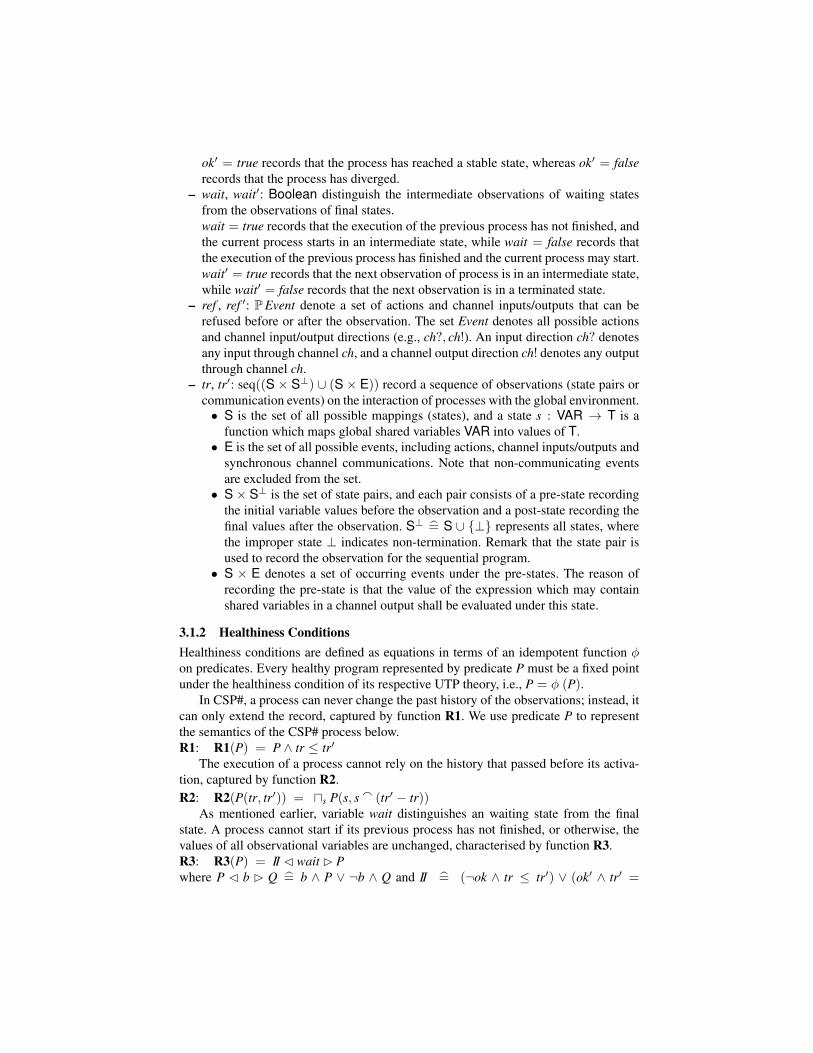
ok′ = true records that the process has reached a stable state, whereas ok′ = falserecords that the process has diverged.

– wait, wait′: Boolean distinguish the intermediate observations of waiting statesfrom the observations of final states.wait = true records that the execution of the previous process has not finished, andthe current process starts in an intermediate state, while wait = false records thatthe execution of the previous process has finished and the current process may start.wait′ = true records that the next observation of process is in an intermediate state,while wait′ = false records that the next observation is in a terminated state.

– ref , ref ′: PEvent denote a set of actions and channel inputs/outputs that can berefused before or after the observation. The set Event denotes all possible actionsand channel input/output directions (e.g., ch?, ch!). An input direction ch? denotesany input through channel ch, and a channel output direction ch! denotes any outputthrough channel ch.

– tr, tr′: seq((S × S⊥) ∪ (S × E)) record a sequence of observations (state pairs orcommunication events) on the interaction of processes with the global environment.• S is the set of all possible mappings (states), and a state s : VAR → T is a

function which maps global shared variables VAR into values of T.• E is the set of all possible events, including actions, channel inputs/outputs and

synchronous channel communications. Note that non-communicating eventsare excluded from the set.

• S× S⊥ is the set of state pairs, and each pair consists of a pre-state recordingthe initial variable values before the observation and a post-state recording thefinal values after the observation. S⊥ =̂ S ∪ {⊥} represents all states, wherethe improper state ⊥ indicates non-termination. Remark that the state pair isused to record the observation for the sequential program.

• S × E denotes a set of occurring events under the pre-states. The reason ofrecording the pre-state is that the value of the expression which may containshared variables in a channel output shall be evaluated under this state.

3.1.2 Healthiness ConditionsHealthiness conditions are defined as equations in terms of an idempotent function φon predicates. Every healthy program represented by predicate P must be a fixed pointunder the healthiness condition of its respective UTP theory, i.e., P = φ (P).

In CSP#, a process can never change the past history of the observations; instead, itcan only extend the record, captured by function R1. We use predicate P to representthe semantics of the CSP# process below.R1: R1(P) = P ∧ tr ≤ tr′

The execution of a process cannot rely on the history that passed before its activa-tion, captured by function R2.R2: R2(P(tr, tr′)) = us P(s, s a (tr′ − tr))

As mentioned earlier, variable wait distinguishes an waiting state from the finalstate. A process cannot start if its previous process has not finished, or otherwise, thevalues of all observational variables are unchanged, characterised by function R3.R3: R3(P) = II C wait B Pwhere P C b B Q =̂ b ∧ P ∨ ¬b ∧ Q and II =̂ (¬ok ∧ tr ≤ tr′) ∨ (ok′ ∧ tr′ =

tr ∧ wait′ = wait ∧ ref ′ = ref ). Here II states that if a process is in a divergent state,then only the trace can be extended, or otherwise, it is in a stable state, and the valuesof all observational variables remain unchanged.

When a process is in a divergent state, it can only extend the trace. This feature iscaptured by function CSP1.CSP1: CSP1(P) = (¬ok ∧ tr ≤ tr′) ∨ P

Every process is monotonic in the observational variable ok′. This monotonicityproperty is modelled by function CSP2 which states that if an observation of a processis valid when ok′ is false, then the observation should also be valid when ok′ is true.CSP2: CSP2(P) = P; (ok⇒ ok′ ∧ tr′ = tr ∧ wait′ = wait ∧ ref ′ = ref )

The behaviour of a process does not depend on the initial value of its refusal, cap-tured by function CSP3.CSP3: CSP3(P) = Skip; P

Similarly, when a process terminates or diverges, the value of its final refusal isirrelevant, characterised by function CSP4.CSP4: P = P; Skip

If a deadlocked process refuses some set of events offered by its environment, thenit would still be deadlocked in an environment that offers even fewer events, capturedby function CSP5CSP5: P = P ||| Skip

We below use H to denote all healthiness conditions satisfied by the CSP# process.

H = R1 ◦ R2 ◦ R3 ◦ CSP1 ◦ CSP2 ◦ CSP3 ◦ CSP4 ◦ CSP5

From the above definition, we can see that although CSP# satisfies the same healthinessconditions of CSP, observational variables tr, tr′ in our semantic model record addi-tional information for shared variable states. We adopt the same names for the idempo-tent functions used in CSP for consistency. In addition, function H is idempotent andmonotonic [1,6].

3.2 Semantics of Expressions and Programs

In this section, we define the semantics of arithmetic expressions, Boolean expressionsand programs. The definitions will be used in Section 3.3.

Definition 1 (Arithmetic Expression). Let Aexp be the type of arithmetic expres-sions defined in Section 2, the evaluation of the expression is defined as a functionA : Aexp→ (S→ T).

A[[n]](s) = nA[[x]](s) = s(x)A[[exp1 + exp2]](s) = A[[exp1]](s) +A[[exp2]](s)A[[exp1 − exp2]](s) = A[[exp1]](s)−A[[exp2]](s)A[[exp1 ∗ exp2]](s) = A[[exp1]](s) ∗ A[[exp2]](s)A[[exp1/exp2]](s) = A[[exp1]](s)/A[[exp2]](s)3

3 We assume the expression is well-defined ( i.e., A[[exp2]](s) 6= 0).

Definition 2 (Boolean Expression). Let Bexp be the type of Boolean expressions de-fined in Section 2, given a valuation, function B returns whether a boolean expressionis valid, defined as B : Bexp→ (S→ Boolean).

B[[true]](s) = trueB[[false]](s) = false

B[[exp1 op exp2)]](s) ={

true A[[exp1]](s) op A[[exp2]](s)false otherwise

B[[¬b]](s) = ¬(B[[b]](s))B[[b1 ∧ b2]](s) = B[[b1]](s) ∧ B[[b2]](s)B[[b1 ∨ b2]](s) = B[[b1]](s) ∨ B[[b2]](s)

Definition 3 (Sequential Program). Let Prog be the type of sequential programs,function C returns the updated valuations after executing the program, defined as C :Prog→ (S → S⊥).

C[[x := exp]] = {(s, s[n/x]) | s ∈ S ∧ n = A[[exp]](s)}C[[prog1; prog2]] = {(s, s′) | ∃ s0 ∈ S • (s, s0) ∈ C[[prog1]]

∧(s0, s′) ∈ C[[prog2]]} ∪{(s,⊥) | (s,⊥) ∈ C[[prog1]]}

C[[if b then prog1 else prog2]] = {(s, s′) | B[[b]](s) = true ∧ (s, s′) ∈ C[[prog1]]} ∪{(s, s′) | B[[b]](s) = false ∧ (s, s′) ∈ C[[prog2]]}

C[[while b do prog]] = {(s, s′) | (s, s′) ∈ C[[µX • F(X)]]}

where, F(X) =̂ if b then prog; X else skip, µX • F(X) =̂⋂

n Fn(true), C[[skip]] ={(s, s) | s ∈ S}, and C[[true]] = {(s, s′) | s ∈ S, s′ ∈ S⊥}.

3.3 Process Semantics

In this section, we construct an observation-oriented semantics for all CSP# processoperators based on our proposed UTP semantic model for CSP#. The semantics is de-fined in an open environment; namely, a process may be interfered with by the en-vironment. In Section 3.1.1, we have defined a hybrid trace to record the potentialevents and state transitions in which a process P may engage; for example, the tracetr′ = 〈(s1, s′1)〉 a 〈(s2, a2)〉 describes the transitions of process P. In an open environ-ment, tr′ may contain an (implicit) transition (s′1, s2) as the result of interference by theenvironment where states s′1 and s2 can be different.

In the following, we illustrate our semantic definitions for the complete CSP# lan-guage, and present the refinement definition.

3.3.1 PrimitivesDeadlock process Stop never engages in any event or updates shared variables, and it isalways waiting.

Stop =̂ H(ok′ ∧ tr′ = tr ∧ wait′)

The semantics shows that the trace is unchanged and wait′ is true. In addition, Stoprefuses all events, so the final value of the refusal set, ref ′, is left unconstrained.

Process Skip terminates immediately without any event or state change occurring.

Skip =̂ H(∃ ref • II)

Reactive condition II constrains that if a process terminates, then there is no change onthe trace. The initial refusal of Skip is relevant to its behaviour, defined by the existentialquantifier making the refusal set ref unconstrained. After termination, the refusal setref ′ is also irrelevant, which is specified by the predicate ∃ ref • II.

3.3.2 Synchronous Channel Output/InputIn CSP#, messages can be sent/received synchronously through channels. The synchro-nisation is pair-wise, involving two processes. Specifically, a synchronous channel com-munication ch.exp can take place only if an output ch!exp is enabled and a correspond-ing input ch?m is also ready.

ch!exp→ P =̂ H

ok′ ∧

ch? 6∈ ref ′ ∧ tr′ = trCwait′B∃ s ∈ S • tr′ = tr a 〈(s, ch!A[[exp]](s))〉

; P

The above semantics of synchronous channel output depicts two possible behaviours:when a process is waiting to communicate on channel ch, it cannot refuse any channelinput over ch provided by the environment to perform a channel communication (rep-resented by predicate ch? 6∈ ref ′), and its trace is unchanged; or a process performsthe output through ch and terminates without divergence. Since the environment mayinterfere with the process behaviour and make a transition on the shared variable states,we use state s to denote the initial state before the observation (also named pre-state).The observation of the trace is recorded as a tuple (s, ch!A[[exp]](s)), where the valueof the output message is evaluated under the pre-state s. Here function A defines thesemantics of arithmetic expressions, and its definition is available in Definition 1. Af-ter the output occurs, the process behaves as P. Note that the semantics of sequentialcomposition “; ” is defined in Section 3.3.4.

ch?m→ P(m) =̂ ∃ v ∈ T •

H

ok′ ∧

ch! 6∈ ref ′ ∧ tr′ = trCwait′B∃ s ∈ S • tr′ = tr a 〈(s, ch?v)〉

; P(v)

As shown above, the semantics of synchronous channel input is similar to channel out-put except that when a process is waiting, it cannot refuse any channel output providedby the environment, and after the process receives a message v from channel ch, itstrace is appended with a tuple (s, ch?v). In addition, parameter m cannot be modified inprocess P; namely, it becomes constant-like and its value is replaced by value v.

3.3.3 Data Operation PrefixingIn CSP#, sequential programs are executed atomically together with the occurrence ofan event, called data operation. The updates on shared variables are observed after theexecution of all programs as illustrated below.

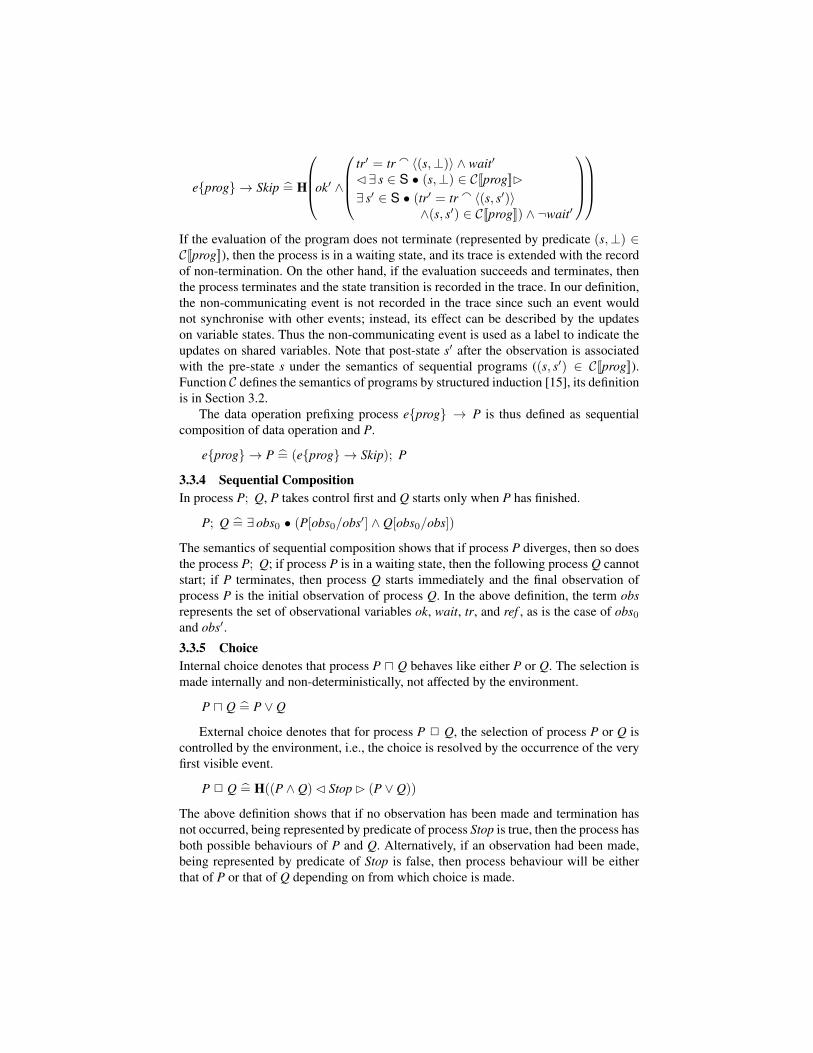
e{prog} → Skip =̂ H

ok′ ∧

tr′ = tr a 〈(s,⊥)〉 ∧ wait′

C∃ s ∈ S • (s,⊥) ∈ C[[prog]]B∃ s′ ∈ S • (tr′ = tr a 〈(s, s′)〉

∧(s, s′) ∈ C[[prog]]) ∧ ¬wait′

If the evaluation of the program does not terminate (represented by predicate (s,⊥) ∈C[[prog]]), then the process is in a waiting state, and its trace is extended with the recordof non-termination. On the other hand, if the evaluation succeeds and terminates, thenthe process terminates and the state transition is recorded in the trace. In our definition,the non-communicating event is not recorded in the trace since such an event wouldnot synchronise with other events; instead, its effect can be described by the updateson variable states. Thus the non-communicating event is used as a label to indicate theupdates on shared variables. Note that post-state s′ after the observation is associatedwith the pre-state s under the semantics of sequential programs ((s, s′) ∈ C[[prog]]).Function C defines the semantics of programs by structured induction [15], its definitionis in Section 3.2.

The data operation prefixing process e{prog} → P is thus defined as sequentialcomposition of data operation and P.

e{prog} → P =̂ (e{prog} → Skip); P

3.3.4 Sequential CompositionIn process P; Q, P takes control first and Q starts only when P has finished.

P; Q =̂ ∃ obs0 • (P[obs0/obs′] ∧ Q[obs0/obs])

The semantics of sequential composition shows that if process P diverges, then so doesthe process P; Q; if process P is in a waiting state, then the following process Q cannotstart; if P terminates, then process Q starts immediately and the final observation ofprocess P is the initial observation of process Q. In the above definition, the term obsrepresents the set of observational variables ok, wait, tr, and ref , as is the case of obs0and obs′.

3.3.5 ChoiceInternal choice denotes that process P u Q behaves like either P or Q. The selection ismade internally and non-deterministically, not affected by the environment.

P u Q =̂ P ∨ Q

External choice denotes that for process P 2 Q, the selection of process P or Q iscontrolled by the environment, i.e., the choice is resolved by the occurrence of the veryfirst visible event.

P 2 Q =̂ H((P ∧ Q)C Stop B (P ∨ Q))

The above definition shows that if no observation has been made and termination hasnot occurred, being represented by predicate of process Stop is true, then the process hasboth possible behaviours of P and Q. Alternatively, if an observation had been made,being represented by predicate of Stop is false, then process behaviour will be eitherthat of P or that of Q depending on from which choice is made.

3.3.6 State Guard

Process [b]P waits until condition b becomes true and then behaves as P. Moreover, thechecking of condition b is performed simultaneously with the occurrence of the firstevent of process P.

[b]P =̂ P / (B(b)(π1(head(tr′ − tr))) = true ∧ tr < tr′) . Stop

The semantics states that if the Boolean guard b is satisfied under the state from theinitial observation of P, being represented by π1(head(tr′ − tr)), then the observationof whole process is the same as P; otherwise, process behaves as Stop process. Thesemantics of Stop is defined in Section 3.3.1. Function π1 selects the first element ofa tuple and head returns the first element of a sequence. Note that the semantics oftraditional conditional choice if (b) {P} else {Q} can be equivalent to the semantics of[b]P ∨ [¬b]Q.

3.3.7 Hiding

The hiding operator makes all occurrences of actions in X not be observed or controlledby the environment of the process. The actions in set X are not recorded in the processtrace.

P \ X =̂ H(∃ s • P[s,X ∪ ref ′/tr′, ref ′] ∧ (tr′ − tr) = hide(s− tr,X)); Skip

The definition of hiding is given by renaming the final trace of P as s, and restricting sto the trace which contains all the events of process P except for those in set X, definedby the function hide. The final refusal set is the union of refusal set of P and set X.

hide : seq((S× E) ∪ (S× S⊥))× PEvent→ seq((S× E) ∪ (S× S⊥))hide(〈 〉) =̂ 〈 〉

hide(〈(s, e)〉a t) =̂{

hide(t,X) if e ∈ X〈(s, e)〉a hide(t,X) otherwise

3.3.8 Parallel Composition

The parallel composition P ‖ Q executes P and Q in the following way: (1) commonactions of P and Q require simultaneous participation, (2) synchronous channel outputin one process occurs simultaneously with the corresponding channel input in the otherprocess, and (3) other events of processes occur independently.

In CSP, the semantics of parallel composition is defined in terms of the merge oper-ator ‖M in UTP [6], where the predicate M captures how to merge two observations. Todeal with channel-based communications and shared variable updates in CSP#, we heredefine a new merge predicate M(X) to model the merge operation. The set X containscommon actions of both processes (denoted by set X1) and all synchronous channelinputs and outputs (denoted by set X2). Namely,

P ‖ Q =̂

(P[0.ok, 0.wait, 0.ref , 0.tr/ok′,wait′, ref ′, tr′] ∧Q[1.ok, 1.wait, 1.ref , 1.tr/ok′,wait′, ref ′, tr′]

); M(X)

where

M(X) =̂

(ok′ = 0.ok ∧ 1.ok) ∧(wait′ = 0.wait ∨ 1.wait) ∧(ref ′ = (0.ref ∩ 1.ref ∩ X2) ∪ ((0.ref ∪ 1.ref ) ∩ X1)

∪ ((0.ref ∩ 1.ref )− X1 − X2))(tr′ − tr ∈ (0.tr − tr ‖X 1.tr − tr))

; Skip

Our defined predicate M(X) captures four kinds of behaviours of a parallel composi-tion. First, the composition diverges if either process diverges (represented by predi-cate ok′ = 0.ok ∧ 1.ok). Second, the composition terminates if both processes termi-nate (wait′ = 0.wait ∨ 1.wait). Third, the composition refuses synchronous channelouputs/inputs that are refused by both processes (0.ref ∩ 1.ref ∩X2), all actions that arein the set X1 and refused by either process ((0.ref ∪1.ref )∩X1), and actions that are notin the set X1 but refused by both processes ((0.ref ∩1.ref )−X1−X2). Last, the trace ofthe composition is a member of the set of traces produced by the trace synchronisationfunction ‖X as elaborated below.

Function ‖X models how to merge two individual traces into a set of all possibletraces; there are 9 cases from 6 groups. In the following definitions, s, s′, s1, s′1, s2, s′2are representative elements of variable states, a, a1, a2 are representative elements ofactions, ch is a representative element of channel names, and v is a value with type T.

– When one of the input traces is empty, (1) if both input traces are empty, the resultis a set of an empty sequence (denoted by case-1); (2) if only one input trace isempty, the result is determined based on the first observation of that non-emptytrace: (i) if that observation is an action in the set X which requires synchronisation,then the result is a set containing only an empty sequence, or otherwise, the firstobservation is recorded in the merged trace (case-2); if the first observation is (ii) achannel input/output/communication (case-3) or (iii) a state pair (case-4), then theobservation is recorded in the merged trace.case-1 〈 〉 ‖X 〈 〉 = {〈 〉}

case-2 〈(s, a)〉a t ‖X 〈 〉 ={{〈 〉} if a ∈ X{〈(s, a)〉a l | l ∈ t ‖X 〈 〉} otherwise

case-3 〈(s, h)〉at ‖X 〈 〉 = {〈(s, h)〉al | l ∈ t ‖X 〈 〉}, where h ∈ {ch?v, ch!v, ch.v}case-4 〈(s, s′)〉a t ‖X 〈 〉 = {〈(s, s′)〉a l | l ∈ t ‖X 〈 〉}

– When a communication is over a synchronous channel, (1) if the first observationsof two input traces match (see Definition 4 below), then a synchronisation mayoccur (denoted by the set G1) or at this moment a synchronisation does not occur(denoted by the set G2), or otherwise, a synchronisation cannot occur. Here, twoobservations are matched provided that both channel input and output from twoprocesses respectively are enabled under the same pre-state.

Definition 4 (Match). Given two pairs p1 = (s1, h1) and p2 = (s2, h2), we saythat they are matched if both s1 = s2 and {h1, h2} = {ch?v, ch!v} are satisfied,denoted as match(p1, p2).

case-5 〈(s1, h1)〉a t1 ‖X 〈(s2, h2)〉a t2 =

{G1 ∪ G2 match((s1, h1), (s2, h2))G2 otherwise

where h1, h2 ∈ {ch?v, ch!v, ch.v}, G1 =̂ {〈(s1, ch.v)〉a l | l ∈ t1 ‖X t2}, and G2 =̂

{〈(s1, h1)〉al | l ∈ t1 ‖X 〈(s2, h2)〉at2}∪{〈(s2, h2)〉al | l ∈ 〈(s1, h1)〉at1 ‖X t2}.– When two actions (a1 and a2) are synchronised, there are five cases with respect

to the initial states (s1 and s2) and actions from the first observation of two inputtraces: (1) both actions are in the set X but different, (2) actions from X are the samebut under different pre-states, (3) actions from X are the same and under the samepre-state, (4) one of the actions is not in X, and (5) both actions are not in X. Asshown in case-6 below, the result is a set containing only an empty sequence forcases (1) and (2). A synchronisation occurs under case (3), although it is postponedto occur under case (4). Either action can occur for case (5).case-6 〈(s1, a1)〉a t1 ‖X 〈(s2, a2)〉a t2 =

{〈 〉} a1, a2 ∈ X ∧ a1 6= a2{〈 〉} a1, a2 ∈ X ∧ a1 = a2 ∧ s1 6= s2{〈(s1, a1)〉a l | l ∈ t1 ‖X t2} a1, a2 ∈ X ∧ a1 = a2 ∧ s1 = s2{〈(s1, a1)〉a l | l ∈ t1 ‖X 〈(s2, a2)〉a t2} a1 6∈ X ∧ a2 ∈ X{〈(s1, a1)〉a l | l ∈ t1 ‖X 〈(s2, a2)〉a t2}∪{〈(s2, a2)〉a l | l ∈ 〈(s1, a1)〉a t1 ‖X t2}

a1 6∈ X ∧ a2 6∈ X

– When the merge operation is on an action a and channel input ch?v, output ch!v,communication ch.v, or a post-state s′2, (1) if a is from the set X, then its occurrenceis postponed (G3), (2) or otherwise, either observation from two processes occurs(G3 ∪ G4).

case-7 〈(s1, a)〉a t1 ‖X 〈(s2, h)〉a t2 =

{G3 if a ∈ XG3 ∪ G4 otherwise

where h ∈ {ch?v, ch!v, ch.v, s′2}, G3 =̂ {〈(s2, h)〉a l | l ∈ 〈(s1, a)〉a t1 ‖X t2}, andG4 =̂ {〈(s1, a)〉a l | l ∈ t1 ‖X 〈(s2, h)〉a t2}.

– When the merge operation is over two state pairs or the operation is on a statepair and a channel input/output/communication, either observation from two pro-cesses can occur as only one process can update shared variable(s) at a time whenprocesses run in parallel.case-8 〈(s1, s′1)〉 a t1 ‖X 〈(s2, h)〉 a t2 = {〈(s1, s′1)〉 a l | l ∈ t1 ‖X 〈(s2, h)〉 a

t2} ∪ {〈(s2, h)〉a l | l ∈ 〈(s1, s′1)〉a t1 ‖X t2} where h ∈ {s′2, ch?v, ch!v, ch.v}– Finally , function ‖X is symmetric.

case-9 t1 ‖X t2 = t2 ‖X t1

3.3.9 InterleaveProcess P ||| Q runs all processes independently (except communications through syn-chronous channels). The semantics of the interleave operator defined below is similarto that of parallel operator except the set X which only contains synchronous channeloutputs and inputs.

P ||| Q =̂ P ‖M(X) Q

The merge predicate M(X) is the same as the definition in section 3.3.8.

3.3.10 Recursion

We have proved that all the process operators in our language are monotonic (see Ap-pendix A). For a recursion process P = µ p • P, the semantics of the weakest fixed pointis the greatest lower bound of all the fixed points with the bottom element H(true) andthe top element H(false), namely, u{X | X w F(X)}. The definition of refinement orderw is shown in Definition 5.

3.3.11 Refinement

Refinement calculus is designed to produce correct programs, assisting in the softwaredevelopment. In the UTP theory, it is expressed as logic implication; an implementation(denoted as predicate P) satisfying a specification (denoted as predicate S) is formallyexpressed by universal quantification implication ∀ a, a′, · · · • P⇒ Q, where a, a′, · · ·are all the variables of the alphabet, which must be the same for the specification andimplementation. The universal quantification implication is usually denoted as [P ⇒Q]. The definition of refinement in CSP# is given as below.

Definition 5 (Refinement). Let P and Q be predicates for processes with the sameshared variable state space, the refinement P w Q holds iff [P⇒ Q].

The refinement ordering in our definition is strong; every observation that satisfies Pmust also satisfy Q. The observation includes all process behaviours, i.e., stability, ter-mination, traces, and refusals. Moreover, the record of the trace considers both variablestates and event occurrences. For example, given a process P = [x = 2]b → Skip 2

[x 6= 2]c → Skip, and a process Q = [x = 2]b → Skip 2 [x 6= 2]d → Skip, the re-finement P w Q does not hold although one observation satisfies both processes whenx is equal to 2. A counterexample is that when x is not equal to 2, processes P and Qperform action c and d, respectively.

Notice that we only allow that in the trace sequence of process P, every element shallbe the same as its counterpart in Q. In other words, our refinement prevents atomic pro-gram operations updating shared variables from being refined by non-atomic programoperations which make the same effect. For example, given a process P = e{x =x + 1} → e{x = x + 1} → Skip, and a process Q = e{x = x + 2} → Skip, therefinement P w Q does not hold.

Definition 6 (Equivalence). For any two CSP# processes P and Q, P is equivalent toQ if and only if P w Q ∧ Q w P.

Lemma 1. All process combinators defined in the CSP# language are monotonic.

The proofs of Lemma 1 is in Appendix A.

Theorem 1. The open semantics of CSP# is compositional.

Proof Given process combinator F and processes P,Q such that P and Q are equivalentwith respect to the open semantics, we have P w Q and Q w P according to Definition6. According to Lemma 1, both F(P) w F(Q) and F(Q) w F(P), which indicatesF(P) = F(Q), i.e., the open semantics is compositional. 2

4 Algebraic Laws

In this section, we present a set of algebraic laws concerning the distinct features ofCSP#. All algebraic laws can be established based on our denotational model. Thatis to say, if the equality of two differently written processes is algebraically provable,then the two processes are also equivalent with respect to the denotational semantics.Moreover, these algebraic laws can be used as auxiliary reasoning rules to provide aneasier way to prove process equivalence during the theorem proving procedures. PATselectively adopts some rules (e.g., seq - 5, par - 3) to speed up the verification bysimplifying the complicated process to the equivalent simpler form.State Guardguard - 1 [b1]([b2]P) = [b1 ∧ b2]Pguard - 2 [b](P1 op P2) = [b]P1 op [b]P2 where, op ∈ {‖,2,u}guard - 3 [false]P = Stopguard - 4 [true]P = Pguard - 1 enables the elimination of nested guards. guard - 2 shows the distribution ofthe state guard through parallel composition, external choice and internal choice. guard- 3 shows that process [false]P behaves like Stop because its guard can never be fired.guard - 4 shows that process [true]P always activates the process P. The proof of theselaws is in Appendix B.

Sequential Compositionseq - 1 (P1; P2); P3 = P1; (P2; P3)seq - 2 P1; (P2 u P3) = (P1; P2) u (P1; P3)seq - 3 (P1 u P2); P3 = (P1; P3) u (P2; P3)seq - 4 P = Skip; Pseq - 5 P = P; Skipseq - 1 shows that sequential composition is associative. seq - 2, 3 show the distributionof sequential composition through external choice. seq - 4, 5 show that process Skip isthe left and right unit of sequential composition, respectively. The semantics of CSP#sequential composition and Skip is the same as in CSP, so the proof of the above lawsis not shown in this report.

Parallel Compositionpar - 1 P1 ‖ P2 = P2 ‖ P1

par - 2 (P1 ‖ P2) ‖ P3 = P1 ‖ (P2 ‖ P3)par - 3 Skip ‖ P = P = P ‖ Skippar - 1, 2 show that parallel composition is commutative and associative. Consequently,the order of parallel composition is irrelevant. par - 3 shows that process Skip is the unitof parallelism. The proof is shown in Appendix B.

5 The Closed Semantics

So far, we have constructed an open semantics for CSP#. Namely, the denotationalsemantics is defined in an open environment. The interference by the environment is

implicitly captured in the hybrid trace which collects the potential events or state tran-sitions in which a process may engage. For example, given a trace 〈(s1, s′1)〉a 〈(s2, e)〉,the transition from state s′1 to s2 is implicit, and it is performed by the environment. Inaddition, the environment can change the states, so it is not necessary to ensure that states′1 is the same as s2. Thus the system and environment alternate in making transitions.From Theorem 1, the open semantics maintains the compositionality of the processes.Therefore, it supports compositional verification of process behaviours.

However, if we look at it in another light, there is no need to retain all possibletransitions from the environment if we have already built the model of the whole systemor the behaviour of the environment has been modelled as a process. In this situation, weattempt to consider a closed semantics for the CSP# language. Fortunately, the closedsemantics does not need to be defined from the scratch; it can be generated from theopen semantics. Thus, we first introduce the definition of closed traces to judge whichtrace exactly describes the process behaviour in a closed environment.

Definition 7 (Closed Trace). A hybrid trace tr is closed, represented as cl(tr), if it sat-isfies the following two conditions.

(1) For any state pair which is not the last element in the trace, the post-state ispassed as the pre-state of its immediate subsequent element, i.e., ∀ 0 ≤ i < #tr −1,∃ s, s′ ∈ S • (tri = (s, s′)⇒ s′ = π1(tr(i+1)))

4.

(2) For any event which is not the last element in the trace, it should share the samepre-state with its immediate subsequent element, i.e., ∀ 0 ≤ i < #tr − 1,∃ s ∈ S, a ∈E • (tri = (s, a)⇒ s = π1(tr(i+1))).

Informally speaking, a closed trace has this property: two adjacent elements in thetrace are associated by a common state; the post-state of the former equals to the pre-state of the latter if the former is a state transition; the pre-state is shared if the formeris an event. Note that every element in a hybrid trace has a pre-state but only the statetransition possesses a post-state because the pre-state is not changed when an eventoccurs. Since the environment cannot update the shared state, a closed trace is identifiedas the behaviour of the process in the closed environment. For convenience, given a setof hybrid traces, denoted as the set HT , we define CL(HT) to represent the set of allclosed traces in HT . Obviously, we have CL(HT) ⊆ HT .

Now, we can generate the closed semantics (denoted by [[P]]closed) from the opensemantics ([[P]]open) for any communicating process P. The relation between them isrevealed by Definition 8.

Definition 8 (Closed Semantics). [[P]]closed =̂ [[P]]open ∧ cl(tr) ∧ cl(tr′)

According to the open semantics, two processes that are semantically equivalent cangenerate the same traces tr, tr′. Further, any two closed traces generated from their opentraces are the same. Thus the equality with respect to the open semantics is preservedby the closed semantics, which is shown in Theorem 2.

Theorem 2. [[P]]open = [[Q]]open ⇒ [[P]]closed = [[Q]]closed

4 tri returns the (i + 1)th element of the sequence tr.

However, we cannot imply that [[P]]open = [[Q]]open is true when [[P]]closed = [[Q]]closed

holds. Furthermore, given that [[P]]closed = [[Q]]closed, the law P ‖ R = Q ‖ R may beinvalid; the compositionality fails in the closed semantics as shown by Example 1.

Example 1. Given a process P = a{x = 2} → ([x = 2]b→ Skip 2 [x 6= 2]c→ Skip),and a process Q = a{x = 2} → ([x = 2]b → Skip 2 [x 6= 2]d → Skip), the closedsemantics of processes P and Q is the same, while their open semantics is not the samebecause after executing the event a, process P may execute event c, and process Qmay execute event d when the value of variable x is not equal to 2 in their pre-states.Therefore, given a process R = e{x = 3} → Skip, there is a case that after executingthe events a and e sequentially, process P ‖ R will execute event c while process Q ‖ Rwill execute event d, and thus the law P ‖ R = Q ‖ R is not satisfied.

6 Conclusion

In this work, we have proposed an observation-oriented semantics in an open environ-ment for the CSP# language based on the UTP framework. The formalised semanticscovers different types of concurrency, i.e., communications and shared variable paral-lelism. In addition, a set of algebraic laws have been proposed based on the denota-tional model for communicating processes involving shared variables. Furthermore, aclosed semantics has been derived from the open denotational semantics by focusingon the particular hybrid traces. Our next step is to encode our proposed semantics intoa generic theorem prover and in turn to validate the algebraic laws using the theoremproving techniques. Ultimately, we can verify the correctness of system behaviours ina theorem prover which may solve the common state space explosion problem.

Acknowledgements

The authors thank Jim Woodcock for insightful comments in the initial discussion.

References

1. A. Cavalcanti and J. Woodcock. A Tutorial Introduction to CSP in Unifying Theories ofProgramming. In PSSE, pages 220–268, 2004.

2. R. Colvin and I. J. Hayes. CSP with Hierarchical State. In IFM, pages 118–135, 2009.3. C. Fischer. Combining Object-Z and CSP. In FBT, pages 119–128, 1997.4. A. J. Galloway and W. J. Stoddart. An Operational Semantics for ZCCS. In ICFEM, pages

272–282, 1997.5. C. Hoare. Communicating Sequential Processes. Prentice-Hall, 1985.6. C. Hoare and J. He. Unifying Theories of Programming. Prentice-Hall, 1998.7. M. Oliveira, A. Cavalcanti, and J. Woodcock. A UTP Semantics for Circus. Formal Asp.

Comput., 21(1-2):3–32, 2009.8. S. Qin, J. S. Dong, and W.-N. Chin. A Semantic Foundation for TCOZ in Unifying Theories

of Programming. In FME, pages 321–340, 2003.9. A. W. Roscoe. The Theory and Practice of Concurrency. Prentice Hall, 1997.

10. S. Schneider and H. Treharne. CSP Theorems for Communicating B Machines. Formal Asp.Comput., 17(4):390–422, 2005.

11. G. Smith. A Semantic Integration of Object-Z and CSP for the Specification of ConcurrentSystems. In FME, pages 62–81, 1997.

12. J. Sun, Y. Liu, J. S. Dong, and C. Chen. Integrating Specification and Programs for SystemModeling and Verification. In TASE, pages 127–135, 2009.

13. J. Sun, Y. Liu, J. S. Dong, and J. Pang. PAT: Towards Flexible Verification under Fairness.In CAV, pages 709–714, 2009.

14. K. Taguchi and K. Araki. The State-Based CCS Semantics for Concurrent Z Specification.In ICFEM, pages 283–292, 1997.

15. G. Winskel. The Formal Semantics of Programming Languages: An Introduction. MIT Press,Cambridge, MA, USA, 1993.

16. J. Woodcock, P. G. Larsen, J. Bicarregui, and J. S. Fitzgerald. Formal Methods: Practice andExperience. ACM Comput. Surv., 41(4), 2009.

17. H. Zhu, J. P. Bowen, and J. He. From Operational Semantics to Denotational Semantics forVerilog. In CHARME, pages 449–466, 2001.

18. H. Zhu, S. Qin, J. He, and J. P. Bowen. PTSC: probability, time and shared-variable concur-rency. ISSE, 5(4):271–284, 2009.

19. H. Zhu, F. Yang, J. He, J. P. Bowen, J. W. Sanders, and S. Qin. Linking Operational Seman-tics and Algebraic Semantics for a Probabilistic Timed Shared-Variable Language. J. Log.Algebr. Program., 81(1):2–25, 2012.

APPENDIX

A Monotonicity of CSP# Process Constructs

In this section, we present the detailed proof of the monotonicity of the CSP# processconstructs. We Given any two processes P and Q such that P w Q, then given any pro-cess Q, the following auxiliary laws should be satisfied.

Law A.1

(P ∧ R) w (Q ∧ R), provided that P w Q.

Proof:

(P ∧ R) w (Q ∧ R) [w]= [(P ∧ R)⇒ (Q ∧ R)] [propositional calculus]= [((P ∧ R)⇒ Q) ∧ ((P ∧ R)⇒ R)] [propositional calculus]= [((P⇒ Q) ∨ (R⇒ Q)) ∧ ((P⇒ R) ∨ (R⇒ R))] [assumption]= [(true ∨ (R⇒ Q)) ∧ ((P⇒ R) ∨ (R⇒ R))] [propositional calculus]= [true ∧ true] [propositional calculus]= true 2

Law A.2

(P ∨ R) w (Q ∨ R), provided that P w Q.

Proof:

(P ∨ R) w (Q ∨ R) [w]= [(P ∨ R)⇒ (Q ∨ R)] [propositional calculus]= [(P⇒ (Q ∨ R)) ∧ (R⇒ (Q ∨ R))] [propositional calculus]= [((P⇒ Q) ∨ (P⇒ R)) ∧ ((R⇒ Q) ∨ (R⇒ R))] [assumption]= [true ∨ (P⇒ R)) ∧ ((R⇒ Q) ∨ (R⇒ R))] [propositional calculus]= [true ∧ true] [propositional calculus]= true 2

The CSP# sequential composition construct is monotonic (see Law A.3 and Law A.4).

Law A.3

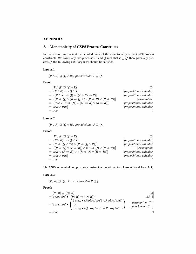
(P; R) w (Q; R), provided that P w Q.

Proof:

(P; R) w (Q; R) [w]= ∀ obs, obs′ • ((P; R)⇒ (Q; R))5 [3.3.4]

= ∀ obs, obs′ •

∃ obs0 • (P[obs0/obs′] ∧ R[obs0/obs])⇒∃ obs0 • (Q[obs0/obs′] ∧ R[obs0/obs])

[assumption, wand Lemma 2

]= true 2

Lemma 2. ∀ obs, obs′•(∃m•(P(obs,m)∧R(m, obs′))⇒ ∃m•(Q(obs,m)∧R(m, obs′)))holds, provided that ∀ obs, obs′ • (P(obs, obs′)⇒ Q(obs, obs′)).

Proof:1 ∀ obs, obs′ • (P(obs, obs′)⇒ Q(obs, obs′)) premise2 obs1 ∀ obs′ • (P(obs1, obs′)⇒ Q(obs1, obs′)) ∀ obs e 13 obs′1 P(obs1, obs′1)⇒ Q(obs1, obs′1) ∀ obs′ e 24 ∃m • (P(obs1,m) ∧ R(m, obs′1)) assumption5 m0 P(obs1,m0) ∧ R(m0, obs′1) ∃m e 46 P(obs1,m0)⇒ Q(obs1,m0) ∀ obs′ e 27 P(obs1,m0) ∧e1 58 Q(obs1,m0) ⇒e 6, 79 R(m0, obs′1) ∧e2 510 Q(obs1,m0) ∧ R(m0, obs′1) ∧i 8, 911 ∃m • (Q(obs1,m) ∧ R(m, obs′1)) ∃m i 1012 ∃m • (Q(obs1,m) ∧ R(m, obs′1)) ∃m 4, 5− 1113 ∃m • (P(obs1,m) ∧ R(m, obs′1))⇒

∃m • (Q(obs1,m) ∧ R(m, obs′1)) ⇒ i 4− 1214 ∀ obs′ • (∃m • (P(obs1,m) ∧ R(m, obs′))⇒

∃m • (Q(obs1,m) ∧ R(m, obs′))) ∀ obs′ i 3− 1315 ∀ obs, obs′ • (∃m • (P(obs,m) ∧ R(m, obs′))⇒

∃m • (Q(obs,m) ∧ R(m, obs′))) ∀ obs i 2− 14Law A.4

(R; P) w (R; Q), provided that P w Q.

Proof:

(R; P) w (R; Q) [w]= ∀ obs, obs′ • ((R; P)⇒ (R; Q)) [3.3.4]

= ∀ obs, obs′ •

∃ obs0 • (R[obs0/obs′] ∧ P[obs0/obs])⇒∃ obs0 • (R[obs0/obs′] ∧ Q[obs0/obs])

[assumption, wand Lemma 3

]= true 2

Lemma 3. ∀ obs, obs′•(∃m•(R(obs,m)∧P(m, obs′))⇒ ∃m•(R(obs,m)∧P(m, obs′)))holds, provided that ∀ obs, obs′ • (P(obs, obs′)⇒ Q(obs, obs′)).

Proof:

5 The term obs represents the set of observational variables ok, wait, tr, as is the case of obs′.

1 ∀ obs, obs′ • (P(obs, obs′)⇒ Q(obs, obs′)) premise2 obs′1 ∀ obs • (P(obs, obs′1)⇒ Q(obs, obs′1)) ∀ obs′ e 13 obs1 P(obs1, obs′1)⇒ Q(obs1, obs′1) ∀ obs e 24 ∃m • (R(obs1,m) ∧ P(m, obs′1)) assumption5 m0 R(obs1,m0) ∧ P(m0, obs′1) ∃m e 46 P(m0, obs′1)⇒ Q(m0, obs′1) ∀ obs e 27 P(m0, obs′1) ∧e2 58 Q(m0, obs′1) ⇒e 6, 79 R(obs1,m0) ∧e1 510 R(obs1,m0) ∧ Q(m0, obs′1) ∧i 8, 911 ∃m • (R(obs1,m) ∧ Q(m, obs′1)) ∃m i 1012 ∃m • (R(obs1,m) ∧ Q(m, obs′1)) ∃m 4, 5− 1113 ∃m • (R(obs1,m) ∧ P(m, obs′1))⇒

∃m • (R(obs1,m) ∧ Q(m, obs′1)) ⇒ i 4− 1214 ∀ obs • (∃m • (R(obs,m) ∧ P(m, obs′1))⇒

∃m • (R(obs,m) ∧ Q(m, obs′1))) ∀ obs i 3− 1315 ∀ obs, obs′ • (∃m • (R(obs,m) ∧ P(m, obs′))⇒

∃m • (R(obs,m) ∧ Q(m, obs′))) ∀ obs′ i 2− 14

Synchronous output/input is monotonic (see Law A.5 and Law A.6).

Law A.5

(ch!exp→ P) w (ch!exp→ Q), provided that P w Q.

Proof:(ch!exp→ P) [3.3.2]

= H

ok′ ∧

ch? 6∈ ref ′ ∧ tr′ = trCwait′B∃ s ∈ S • tr′ = tr a 〈(s, ch!A[[exp]](s))〉

; P[

assumptionand A.4

]

w H

ok′ ∧

ch? 6∈ ref ′ ∧ tr′ = trCwait′B∃ s ∈ S • tr′ = tr a 〈(s, ch!A[[exp]](s))〉

; Q [3.3.2]

= ch!exp→ Q 2

Law A.6

(ch?m→ P(m)) w (ch?m→ Q(m)), provided that ∀m ∈ T • P(m) w Q(m).

Proof:ch?m→ P(m) [3.3.2]

= ∃ v ∈ T •

H

ok′ ∧

ch! 6∈ ref ′ ∧ tr′ = trCwait′Btr′ = tr a 〈(s, ch?v)〉

; P(v)

assumption, A.4,and predicatecalculus

w ∃ v ∈ T •

H

ok′ ∧

ch! 6∈ ref ′ ∧ tr′ = trCwait′Btr′ = tr a 〈(s, ch?v)〉

; Q(v)

[3.3.2]

= ch?m→ Q(m) 2

The CSP# data operation prefixing construct is monotonic (see Law A.7).

Law A.7

(e{prog} → P) w (e{prog} → Q), provided that P w Q.

Proof:e{prog} → P [3.3.3]

= H

ok′ ∧

∃ s ∈ S • (tr′ = tr a 〈(s,⊥)〉 ∧ (s,⊥) ∈ C[[prog]])Cwait′B∃ s, s′ ∈ S • (tr′ = tr a 〈(s, s′)〉 ∧ (s, s′) ∈ C[[prog]]∧(s,⊥) 6∈ C[[prog]])

; P

[assumptionand A.4

]

w H

ok′ ∧

∃ s ∈ S • (tr′ = tr a 〈(s,⊥)〉 ∧ (s,⊥) ∈ C[[prog]])Cwait′B∃ s, s′ ∈ S • (tr′ = tr a 〈(s, s′)〉 ∧ (s, s′) ∈ C[[prog]]∧(s,⊥) 6∈ C[[prog]])

; Q [3.3.3]

= e{prog} → Q 2

The CSP# state guard is monotonic (see Law A.8).

Law A.8

[b]P w [b]Q, provided that P w Q.

Proof:[b]P w [b]Q [3.3.6 and w]

=

P / B(b)(π1(head(tr′ − tr))) = true ∧ tr < tr′) . Stop⇒Q / B(b)(π1(head(tr′ − tr))) = true ∧ tr < tr′) . Stop

[predicatecalculus

]

=

(P ∧ B(b)(π1(head(tr′ − tr))) = true ∧ tr < tr′)⇒(Q ∧ B(b)(π1(head(tr′ − tr))) = true ∧ tr < tr′)

∨ (P ∧ B(b)(π1(head(tr′ − tr))) = true ∧ tr < tr′)⇒(Stop ∧ ¬(B(b)(π1(head(tr′ − tr))) = true ∧ tr < tr′))

∧

(Stop ∧ ¬(B(b)(π1(head(tr′ − tr))) = true ∧ tr < tr′))⇒(Q ∧ B(b)(π1(head(tr′ − tr))) = true ∧ tr < tr′)

∨ (Stop ∧ ¬(B(b)(π1(head(tr′ − tr))) = true ∧ tr < tr′))⇒(Stop ∧ ¬(B(b)(π1(head(tr′ − tr))) = true ∧ tr < tr′))

[predicatecalculus

]

=

(P⇒ Q)∨

((B(b)(π1(head(tr′ − tr))) = true ∧ tr < tr′)⇒ Q)∨ (P ∧ B(b)(π1(head(tr′ − tr))) = true ∧ tr < tr′)⇒(Stop ∧ ¬(B(b)(π1(head(tr′ − tr))) = true ∧ tr < tr′))

∧ (Stop ∧ ¬(B(b)(π1(head(tr′ − tr))) = true ∧ tr < tr′))⇒(Q ∧ B(b)(π1(head(tr′ − tr))) = true ∧ tr < tr′)

∨

true

assumptionandpredicatecalculus

= true ∧ true[

predicatecalculus

]= true 2

The CSP# parallel composition is monotonic (see Law A.9 and Law A.10).

Law A.9

P || R w Q || R

provided that P w Q, and common synchronization events of the two parallel processes(denoted as set X) are the same.Proof:

P w Q [w]= [P⇒ Q] [predicate calculus]= [P[0.obs/obs]⇒ Q[0.obs/obs]] [w]= P[0.obs/obs] w Q[0.obs/obs] [Law A.1]

=(P[0.obs/obs] ∧ R[1.obs/obs])w(Q[0.obs/obs] ∧ R[1.obs/obs])

[Law A.3]

⇒(P[0.obs/obs] ∧ R[1.obs/obs]); M(X)w(Q[0.obs/obs] ∧ R[1.obs/obs]); M(X)

[3.3.8]

= P || R w Q || R 2

Law A.10

R || P w R || Q,

provided that P w Q, and common synchronization events of the two parallel processes(denoted as set X) are the same.

Proof:P w Q [w]

= [P⇒ Q] [predicate calculus]= [P[1.obs/obs]⇒ Q[1.obs/obs]] [w]= P[1.obs/obs] w Q[1.obs/obs] [A.1]

=(P[1.obs/obs] ∧ R[0.obs/obs])w(Q[1.obs/obs] ∧ R[0.obs/obs])

[predicate calculus]

=(R[0.obs/obs] ∧ P[1.obs/obs])w(R[0.obs/obs] ∧ Q[1.obs/obs])

[A.3]

⇒(R[0.obs/obs] ∧ P[1.obs/obs]); M(X)w(R[0.obs/obs] ∧ Q[1.obs/obs]); M(X)

[3.3.8]

= R || P w R || Q 2

Since the semantics of other CSP# processes (i.e., event prefixing, external/internalchoice, hiding and recursion) is the same as that of CSP, the proof is ommited here.

B Proof of Algebraic Laws

In this section, we present the proofs of laws in Section 4.Law guard - 1

[b1]([b2]P) = [b1 ∧ b2]P

Proof:[b1]([b2]P) [3.3.6]

=(P / (B(b2)(π1(head(tr′ − tr))) = true ∧ tr < tr′) . Stop)/(B(b1)(π1(head(tr′ − tr))) = true ∧ tr < tr′) . Stop [predicate calculus]

=

P ∧ B(b2)(π1(head(tr′ − tr))) = true∧tr < tr′∧B(b1)(π1(head(tr′ − tr))) = true

∨Stop ∧ ¬(B(b2)(π1(head(tr′ − tr))) = true∧

tr < tr′∧B(b1)(π1(head(tr′ − tr))) = true)

[Def . 2]

=(P ∧ B(b2 ∧ b1)(π1(head(tr′ − tr))) = true ∧ tr < tr′)∨(Stop ∧ ¬(B(b2 ∧ b1)(π1(head(tr′ − tr))) = true ∧ tr < tr′))

[3.3.6]

= [b1 ∧ b2]P 2

Law guard - 2

[b](P1 op P2) = [b]P1 op [b]P2 where, op ∈ {‖,2,u}

Proof: The guard b1 constrains that the pre-state of initial observation of compositionprocess should satisfies the condition, since the pre-state of the initial observation of thecomposition process can be from either process P1 or P2 (see Section 3.3.5, 3.3.8), sothe condition should be satisfied by the initial observation of both processes. 2

Law guard - 3

[false]P = Stop

Proof:

[false]P [3.3.6]= P / (B(false)(π1(head(tr′ − tr))) = true ∧ tr < tr′) . Stop [Def . 2]= P / (false ∧ tr < tr′) . Stop [predicate calculus]= Stop 2

Law guard - 4

[true]P = P

Proof:

[true]P [3.3.6]

= P / (B(true)(π1(head(tr′ − tr))) = true ∧ tr < tr′) . Stop[

Def . 2 andpredicate calculus

]= P 2

Law par - 1

P1 ‖ P2 = P2 ‖ P1

Proof:

P1 ‖ P2 [3.3.8]

= (P1[0.obs/obs′] ∧ P2[1.obs/obs′]); M(X)[

symmetry of M(X) andpredicate calculus

]= (P2[0.obs/obs′] ∧ P1[1.obs/obs′]); M(X) [3.3.8]= P2 ‖ P1 2

Law par - 2

(P1 ‖ P2) ‖ P3 = P1 ‖ (P2 ‖ P3),

provided that common synchronization events among processes P1, P2 and P3 (denotedas set X) are the same.

Proof:

(P1 ‖ P2) ‖ P3 [3.3.8]

=

((P1[0.obs/obs′] ∧ P2[1.obs/obs′]); M(X))[0.obs/obs′]∧P3[1.obs/obs′]

; M(X)[

associativity of M(X),predicate calculus

]

=

P1[0.obs/obs′]∧((P2[0.obs/obs′] ∧ P3[1.obs/obs′]); M(X))[1.obs/obs′]

; M(X) [3.3.8]

= P1 ‖ (P2 ‖ P3) 2

Law par - 3

Skip ‖ P = P = P ‖ Skip,

given that set X1 is a set of channel outputs and inputs.Proof:

Skip ‖ P [par− 1]= P ‖ Skip 2

P ‖ Skip [3.3.8]= P ‖M(X) Skip [UTP parallel]= ((P[0.obs/obs′]) ∧ (Skip[1.obs/obs′])); M(X1) [3.3.1]= ((P[0.obs/obs′]) ∧ (H(∃ ref • II)[1.obs/obs′])); M(X1) [H]

=

((P[0.obs/obs′]) ∧

(wait ∧ ¬ok ∧ tr ≤ tr′) ∨(wait ∧ ok′ ∧ tr′ = tr ∧ wait′ = wait ∧ ref ′ = ref ) ∨(¬wait ∧ ¬ok ∧ tr ≤ tr′) ∨(¬wait ∧ ∃ ref • (ok′ ∧ tr′ = tr ∧ wait′ = wait∧ ref ′ = ref ))

[1.obs/obs′]

; M(X1)

[propositionalcalculus

]

=

((P[0.obs/obs′]) ∧ (¬ok ∧ tr ≤ tr′) ∨

(wait ∧ ok′ ∧ tr′ = tr ∧ wait′ = wait ∧ ref ′ = ref ) ∨(¬wait ∧ ok′ ∧ tr′ = tr ∧ wait′ = wait)

[1.obs/obs′]

; M(X1) [P is CSP1]

=

((CSP1(P)[0.obs/obs′]) ∧ (¬ok ∧ tr ≤ tr′) ∨

(wait ∧ ok′ ∧ tr′ = tr ∧ wait′ = wait ∧ ref ′ = ref ) ∨(¬wait ∧ ok′ ∧ tr′ = tr ∧ wait′ = wait)

[1.obs/obs′]

; M(X1) [CSP1]

=

((P ∨ ¬ok ∧ tr ≤ tr′)[0.obs/obs′]) ∧ (¬ok ∧ tr ≤ tr′) ∨

(wait ∧ ok′ ∧ tr′ = tr ∧ wait′ = wait ∧ ref ′ = ref ) ∨(¬wait ∧ ok′ ∧ tr′ = tr ∧ wait′ = wait)

[1.obs/obs′]

; M(X1) [P is R3]

=

((R3(P) ∨ ¬ok ∧ tr ≤ tr′)[0.obs/obs′]) ∧ (¬ok ∧ tr ≤ tr′) ∨

(wait ∧ ok′ ∧ tr′ = tr ∧ wait′ = wait ∧ ref ′ = ref ) ∨(¬wait ∧ ok′ ∧ tr′ = tr ∧ wait′ = wait)

[1.obs/obs′]

; M(X1) [R3]

=

wait ∧ II ∨¬wait ∧ P ∨¬ok ∧ tr ≤ tr′

[0.obs/obs′])

∧ (¬ok ∧ tr ≤ tr′) ∨(wait ∧ ok′ ∧ tr′ = tr ∧ wait′ = wait ∧ ref ′ = ref ) ∨(¬wait ∧ ok′ ∧ tr′ = tr ∧ wait′ = wait)

[1.obs/obs′]

; M(X1)

II andprositionalcalculus

=

(¬ok ∧ tr ≤ tr′) ∨(wait ∧ ok′ ∧ tr′ = tr ∧ wait′ = wait ∧ ref ′ = ref ) ∨(¬wait ∧ P)

[0.obs/obs′])

∧ (¬ok ∧ tr ≤ tr′) ∨(wait ∧ ok′ ∧ tr′ = tr ∧ wait′ = wait ∧ ref ′ = ref ) ∨(¬wait ∧ ok′ ∧ tr′ = tr ∧ wait′ = wait)

[1.obs/obs′]

; M(X1)

[predicatecalculus

]

=

(¬ok ∧ tr ≤ 0.tr) ∨(wait ∧ 0.ok ∧ 0.tr = tr ∧ 0.wait = wait ∧ 0.ref = ref ) ∨(¬wait ∧ P[0.obs/obs′])

∧ (¬ok ∧ tr ≤ 1.tr) ∨(wait ∧ 1.ok ∧ 1.tr = tr ∧ 1.wait = wait ∧ 1.ref = ref ) ∨(¬wait ∧ 1.ok ∧ 1.tr = tr ∧ 1.wait = wait)

; M(X1)

[propositionalcalculus

]

=

(¬ok ∧ tr ≤ 0.tr ∧ tr ≤ 1.tr) ∨(¬ok ∧ tr ≤ 0.tr ∧ wait ∧ 1.ok∧ 1.tr = tr ∧ 1.wait = wait ∧ 1.ref = ref ) ∨

(¬ok ∧ tr ≤ 0.tr ∧ ¬wait ∧ 1.ok∧ 1.tr = tr ∧ 1.wait = wait) ∨

(¬ok ∧ tr ≤ 1.tr ∧ wait ∧ 0.ok∧ 0.tr = tr ∧ 0.wait = wait ∧ 0.ref = ref ) ∨

(wait ∧ 0.ok ∧ 1.ok ∧ 0.tr = 1.tr = tr∧ 0.wait = 1.wait = wait ∧ 0.ref = 1.ref = ref ) ∨

(¬ok ∧ tr ≤ 1.tr ∧ ¬wait ∧ (P[0.obs/obs′])) ∨(¬wait ∧ 1.ok ∧ 1.tr = tr ∧ 1.wait = wait ∧ P[0.obs/obs′])

; M(X1) [3.3.8 M(X)]

=

(¬ok ∧ tr ≤ 0.tr ∧ tr ≤ 1.tr) ∨(¬ok ∧ tr ≤ 0.tr ∧ wait ∧ 1.ok∧ 1.tr = tr ∧ 1.wait = wait ∧ 1.ref = ref ) ∨

(¬ok ∧ tr ≤ 0.tr ∧ ¬wait ∧ 1.ok∧ 1.tr = tr ∧ 1.wait = wait) ∨

(¬ok ∧ tr ≤ 1.tr ∧ wait ∧ 0.ok∧ 0.tr = tr ∧ 0.wait = wait ∧ 0.ref = ref ) ∨

(wait ∧ 0.ok ∧ 1.ok ∧ 0.tr = 1.tr = tr∧ 0.wait = 1.wait = wait ∧ 0.ref = 1.ref = ref ) ∨

(¬ok ∧ tr ≤ 1.tr ∧ ¬wait ∧ (P[0.obs/obs′])) ∨(¬wait ∧ 1.ok ∧ 1.tr = tr ∧ 1.wait = wait ∧ (P[0.obs/obs′]))

;

(ok′ = 0.ok ∧ 1.ok) ∧(wait′ = 0.wait ∨ 1.wait) ∧(ref ′ = ((0.refa ∪ 1.refa) ∩ X1) ∪ ((0.refa ∩ 1.refa)− X1)

∪ (0.refc ∩ 1.refc ∩ X2)) ∧(tr′ − tr ∈ (0.tr − tr ‖X 1.tr − tr))

; Skip

[seq− 1]

=

(¬ok ∧ tr ≤ 0.tr ∧ tr ≤ 1.tr) ∨(¬ok ∧ tr ≤ 0.tr ∧ wait ∧ 1.ok∧ 1.tr = tr ∧ 1.wait = wait ∧ 1.ref = ref ) ∨

(¬ok ∧ tr ≤ 0.tr ∧ ¬wait ∧ 1.ok∧ 1.tr = tr ∧ 1.wait = wait) ∨

(¬ok ∧ tr ≤ 1.tr ∧ wait ∧ 0.ok∧ 0.tr = tr ∧ 0.wait = wait ∧ 0.ref = ref ) ∨

(wait ∧ 0.ok ∧ 1.ok ∧ 0.tr = 1.tr = tr∧ 0.wait = 1.wait = wait ∧ 0.ref = 1.ref = ref ) ∨

(¬ok ∧ tr ≤ 1.tr ∧ ¬wait ∧ (P[0.obs/obs′])) ∨(¬wait ∧ 1.ok ∧ 1.tr = tr ∧ 1.wait = wait ∧ (P[0.obs/obs′]))

;(ok′ = 0.ok ∧ 1.ok) ∧(wait′ = 0.wait ∨ 1.wait) ∧(ref ′ = ((0.refa ∪ 1.refa) ∩ X1) ∪ ((0.refa ∩ 1.refa)− X1)

∪ (0.refc ∩ 1.refc ∩ X2)) ∧(tr′ − tr ∈ (0.tr − tr ‖X 1.tr − tr))

; Skip [3.3.4]

=

(¬ok ∧ tr ≤ 0.tr ∧ tr ≤ 1.tr) ∨(¬ok ∧ tr ≤ 0.tr ∧ wait ∧ 1.ok∧ 1.tr = tr ∧ 1.wait = wait ∧ 1.ref = ref ) ∨

(¬ok ∧ tr ≤ 0.tr ∧ ¬wait ∧ 1.ok∧ 1.tr = tr ∧ 1.wait = wait) ∨

(¬ok ∧ tr ≤ 1.tr ∧ wait ∧ 0.ok∧ 0.tr = tr ∧ 0.wait = wait ∧ 0.ref = ref ) ∨

(wait ∧ 0.ok ∧ 1.ok ∧ 0.tr = 1.tr = tr∧ 0.wait = 1.wait = wait ∧ 0.ref = 1.ref = ref ) ∨

(¬ok ∧ tr ≤ 1.tr ∧ ¬wait ∧ (P[0.obs/obs′])) ∨(¬wait ∧ 1.ok ∧ 1.tr = tr ∧ 1.wait = wait ∧ (P[0.obs/obs′]))

∧(ok′ = 0.ok ∧ 1.ok) ∧(wait′ = 0.wait ∨ 1.wait) ∧(ref ′ = ((0.refa ∪ 1.refa) ∩ X1) ∪ ((0.refa ∩ 1.refa)− X1)

∪ (0.refc ∩ 1.refc ∩ X2)) ∧(tr′ − tr ∈ (0.tr − tr ‖X 1.tr − tr))

; Skip[

predicatecalculus

]

=

(¬ok ∧ tr ≤ tr′) ∨(¬ok ∧ wait ∧ tr ≤ tr′ ∧ ok′ = 0.ok ∧ Ψ1) ∨(¬ok ∧ ¬wait ∧ tr ≤ tr′ ∧ wait′ = 0.wait) ∨(¬ok ∧ wait ∧ tr ≤ tr′ ∧ ok′ = 1.ok ∧ Ψ2) ∨(wait ∧ ok′ ∧ tr′ = tr ∧ wait′ = wait ∧ ref ′ = ref ) ∨(¬ok ∧ ¬wait ∧ tr ≤ tr′ ∧ Ψ3) ∨(¬wait ∧ ok′ = 0.ok ∧ tr′ = 0.tr ∧ wait′ = 0.wait∧ ref ′ = 0.ref ∧ (P[0.obs/obs′]))

6; Skip

[predicatecalculus

]

=

(¬ok ∧ tr ≤ tr′) ∨(wait ∧ ok′ ∧ tr′ = tr ∧ wait′ = wait ∧ ref ′ = ref ) ∨(¬wait ∧ P)

; Skip [II]

=

(wait ∧ II) ∨(¬wait ∧ P) ∨(¬ok ∧ tr ≤ tr′)

; Skip [R3]

=

(R3(P) ∨(¬ok ∧ tr ≤ tr′)

); Skip [P is R3]

= (P ∨ ¬ok ∧ tr ≤ tr′); Skip [CSP1]

= CSP1(P); Skip [P is CSP1]

= P; Skip [seq− 5]

= P 2

6 Ψ1, Ψ2 and Ψ3 are logic formulae in terms of ref ′, 0.ref and 1.ref .