Embed Size (px)
Citation preview
Entropy 2007, 9, 1-26
EntropyISSN 1099-4300
www.mdpi.org/entropy/
Full paper
A Utility-Based Approach to Some InformationMeasures
Craig Friedman ∗, Jinggang Huang ◦ and Sven Sandow †
Standard & Poor’s, 55 Water Street, 46th Floor, New York, NY 10041, USA
E-Mail: ∗ craig [email protected], ◦ james [email protected], † [email protected]
Received: 23 May 2006 / Accepted: 5 January 2007 / Published: 20 January 2007
Abstract: We review a decision theoretic, i.e., utility-based, motivation for entropy and Kullback-
Leibler relative entropy, the natural generalizations that follow, and various properties of these
generalized quantities. We then consider these generalized quantities in an easily interpreted spe-
cial case. We show that the resulting quantities, share many of the properties of entropy and
relative entropy, such as the data processing inequality and the second law of thermodynamics.
We formulate an important statistical learning problem – probability estimation – in terms of a
generalized relative entropy. The solution of this problem reflects general risk preferences via the
utility function; moreover, the solution is optimal in a sense of robust absolute performance.
Keywords: Generalized Entropy, Generalized Kullback-Leibler Relative Entropy, Decision The-
ory, Expected Utility, Horse Race, Tsallis Entropy, Statistical Learning, Probability Estimation,
Risk Neutral Pricing Measure
Entropy 2007, 9, 1-26 2
1 Introduction
It is well known that there are a number of ways to motivate the fundamental quantities of
information theory, for example:
• Entropy can be defined as essentially the only quantity that is consistent with a plausible
set of information axioms (the approach taken by Shannon (1948) for a communication
system–see also Csiszar and Korner (1997) for additional axiomatic approaches).
• The definition of entropy is related to the definition of entropy from thermodynamics (see,
for example, Brillouin (1962) and Jaynes (1957)).
There is a substantial literature on various generalizations of entropy, for example, the Tsal-
lis entropy (with an extensive biblioigraphy in Group of Statistical Physics (2006)), which was
introduced by Cressie and Read (1984) and Cressie and Read (1989) and used for statistical de-
cisions. There is a literature on income inequality which generalizes entropy (see, for example,
Cowell (1981)). A generalization of relative entropy, relative Tsallis entropy (alpha-divergence),
was introduced by Liese and Vajda (1987). Osterreicher and Vajda (May, 1993), Stummer (1999),
Stummer (2001), and Stummer (2004) discussed Tsallis entropy and optimal Bayesian decisions.
A number of these generalization are closely related to the material in this paper. In this paper, we
discuss entropy and Kullback-Leibler relative entropy from a decision theoretic point of view; in
particular, we review utility-based motivations and generalizations of these information theoretic
quantities, based on fundamental principles from decision theory applied in a particular ”market”
context. As we shall see, some generalizations share important properties with entropy and relative
entropy. We then formulate a statistical learning problem (estimation of probability measures) in
terms of these generalized quantities and discuss optimality properties of the solution.
The connection between information theoretic quantities and gambling is well known. Cover and
Thomas (1991) (see Theorem 6.1.2), for example, show that in the horse race setting, an expected
wealth growth rate maximizing investor, who correctly understands the probabilities, has expected
wealth growth rate equal to that of a clairvoyant (someone who wins every bet) minus the entropy
of the horse race. Thus, the entropy can be interpreted as the difference between the wealth
growth rates attained by a clairvoyant and an expected wealth growth rate maximizing investor
who allocates according to the true measure p. It follows from Cover and Thomas (1991), Theorem
6.1.2 and Equation (6.13) that an investor who allocates according to the measure q rather than
p, suffers a loss in expected wealth growth rate of Kullback-Leibler relative entropy D(p‖q).
Investors who maximize expected wealth growth rates can be viewed as expected logarithmic
utility maximizers; thus, the entropy can be interpreted as the difference in expected logarithmic
utility attained by a clairvoyant and expected logarithmic utility maximizing investor who allocates
according to the true measure p. By similar reasoning, an investor who allocates according to the
measure q rather than p, suffers a loss in expected logarithmic utility of D(p‖q). Friedman and
Sandow (2003b) extend these ideas and define a generalized entropy and a generalized Kullback-
Leibler relative entropy for investors with general utility functions.
Entropy 2007, 9, 1-26 3
In Section 2, we review the generalizations and various properties of the generalized quantities
introduced in Friedman and Sandow (2003b). In Section 3 we consider these quantities in a new
and natural special case. We show that the resulting quantities, which are still more general than
entropy and Kullback-Leibler relative entropy, share many of the properties of entropy and relative
entropy, for example, the data processing inequality and the second law of thermodynamics. We
note that one of the most popular families of utility functions from finance leads to a monotone
transformation of the Tsallis entropy. In Section 4 we formulate a decision-theoretic approach
to the problem of learning a probability measure from data. This approach, formulated in terms
of the quantities described in Section 3, generalizes the minimum relative entropy approach to
estimating probabilistic models. This more general formulation specifically incorporates the risk
preferences of an investor who would use the probability measure that is to be learned in order to
make decisions in a particular market setting. Moreover, we show that the probability measure
that is “learned” is robust in the sense that an investor allocating according to the “learned”
measure maximizes his expected utility in the most adverse environment consistent with certain
data consistency constraints.
2 (U,O)-Entropy
According to utility theory (see, for example, Theorem 3, p. 31 of Ingersoll (1987)), a rational
investor acts to maximize his expected utility based on the model he believes. Friedman and
Sandow (2003b) use this fact to construct general information theoretic quantities that depend on
the probability measures associated with potential states of a horse race (defined precisely below).
In this section, we review the horse race setting, notions from utility theory and definitions and
some of the basic properties of the generalized entropy ((U,O)−entropy) and the generalized
relative entropy (relative (U,O)-entropy) from Friedman and Sandow (2003b).
2.1 Probabilistic Model and Horse Race
We consider the random variable X with values, x, in a finite set X .1 Let q(x) denote prob{X = x}
under the probability measure q. We adopt the viewpoint of an investor who uses the model to
place bets on a horse race, which we define as follows:2
Definition 1 A horse race is a market characterized by the discrete random variable X with
possible states x ∈ X , where an investor can place a bet that X = x, which pays the odds ratio
O(x) > 0 for each dollar wagered if X = x, and 0, otherwise.
We assume that our investor allocates b(x) to the event X = x, where
∑
x
b(x) = 1. (1)
1We have chosen this setting for the sake of simplicity. One can generalize the ideas in this paper to continuous
random variables and to conditional probability models; for details, see Friedman and Sandow (2003b).2See, for example, Cover and Thomas (1991), Chapter 6.
Entropy 2007, 9, 1-26 4
We note that we have not required b(x) to be nonnegative. For some utility functions, the investor
may choose to “short” a particular horse. We also note that we can ease the constraint (1) so as
to allow our investor to leverage or withhold cash. This will not lead to any significant change in
the final results of this paper (see Friedman and Sandow (2004)).
The investor’s wealth after the bet is
W = b(x)O(x), (2)
where x denotes the winning horse.
We note that an investor who allocates $1 of capital, investing BO(x)
to each state x, where
B =1
∑
x1
O(x)
, (3)
receives the payoff B with certainty. This motivates the following definition:
Definition 2 The riskless bank account payoff, B, is given by
B =1
∑
x1
O(x)
. (4)
In a horse race with superfair odds,3 B > 1; in a horse race with subfair odds (there is a “track
take”), B < 1. In financial markets, with positive “interest rates,” B > 1. If the “interest rate”
is zero, B = 1.
2.2 Utility and Optimal Betting Weights
In order to quantify the benefits, to an investor, of the information in the model q, we consider
the investor’s utility function, U .
Assumption 1 Our investor subscribes to the axioms of utility theory.4 The investor has a utility
function, U : (Wb,Ws) → R, that
(i) is strictly concave,
(ii) is twice differentiable,
(iii) is strictly monotone increasing,
(iv) has the property (0,∞) ⊆ range(U ′), i.e., there exists a ’blow-up point’, Wb, with
limW→W+
b
U ′(W ) = ∞ (5)
and a ’saturation point’, Ws, with
limW→W−
s
U ′(W ) = 0, (6)
and3See, for example, Cover and Thomas (1991).4Such an investor maximizes his expected utility with respect to the probability measure that he believes (see,
for example, Luenberger (1998)).
Entropy 2007, 9, 1-26 5
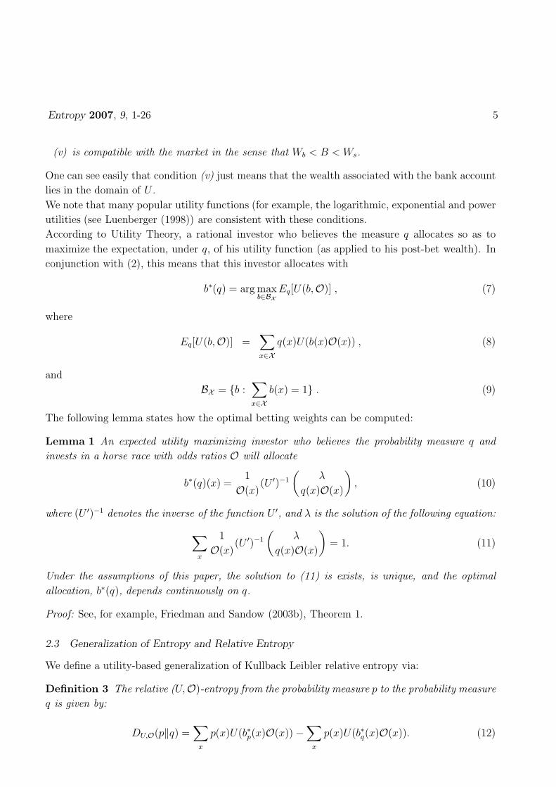
(v) is compatible with the market in the sense that Wb < B < Ws.
One can see easily that condition (v) just means that the wealth associated with the bank account
lies in the domain of U .
We note that many popular utility functions (for example, the logarithmic, exponential and power
utilities (see Luenberger (1998)) are consistent with these conditions.
According to Utility Theory, a rational investor who believes the measure q allocates so as to
maximize the expectation, under q, of his utility function (as applied to his post-bet wealth). In
conjunction with (2), this means that this investor allocates with
b∗(q) = arg maxb∈BX
Eq[U(b,O)] , (7)
where
Eq[U(b,O)] =∑
x∈X
q(x)U(b(x)O(x)) , (8)
and
BX = {b :∑
x∈X
b(x) = 1} . (9)
The following lemma states how the optimal betting weights can be computed:
Lemma 1 An expected utility maximizing investor who believes the probability measure q and
invests in a horse race with odds ratios O will allocate
b∗(q)(x) =1
O(x)(U ′)−1
(
λ
q(x)O(x)
)
, (10)
where (U ′)−1 denotes the inverse of the function U ′, and λ is the solution of the following equation:
∑
x
1
O(x)(U ′)−1
(
λ
q(x)O(x)
)
= 1. (11)
Under the assumptions of this paper, the solution to (11) is exists, is unique, and the optimal
allocation, b∗(q), depends continuously on q.
Proof: See, for example, Friedman and Sandow (2003b), Theorem 1.
2.3 Generalization of Entropy and Relative Entropy
We define a utility-based generalization of Kullback Leibler relative entropy via:
Definition 3 The relative (U,O)-entropy from the probability measure p to the probability measure
q is given by:
DU,O(p‖q) =∑
x
p(x)U(b∗p(x)O(x)) −∑
x
p(x)U(b∗q(x)O(x)). (12)
Entropy 2007, 9, 1-26 6
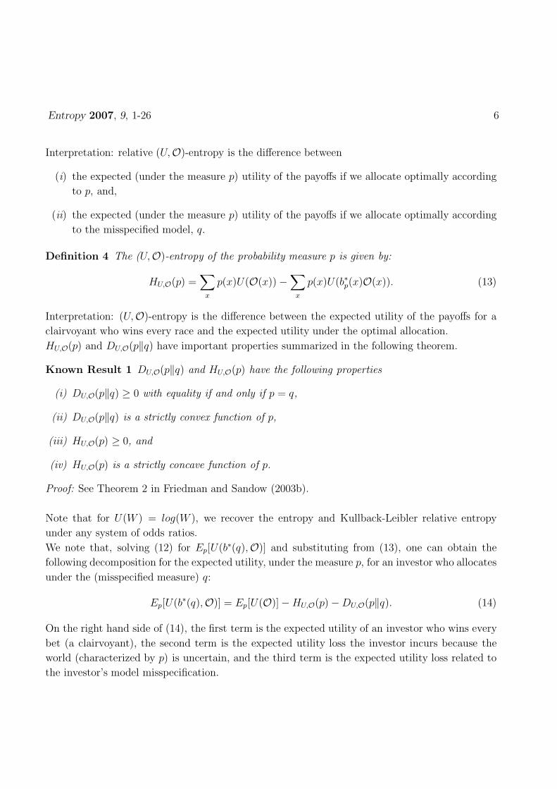
Interpretation: relative (U,O)-entropy is the difference between
(i) the expected (under the measure p) utility of the payoffs if we allocate optimally according
to p, and,
(ii) the expected (under the measure p) utility of the payoffs if we allocate optimally according
to the misspecified model, q.
Definition 4 The (U,O)-entropy of the probability measure p is given by:
HU,O(p) =∑
x
p(x)U(O(x)) −∑
x
p(x)U(b∗p(x)O(x)). (13)
Interpretation: (U,O)-entropy is the difference between the expected utility of the payoffs for a
clairvoyant who wins every race and the expected utility under the optimal allocation.
HU,O(p) and DU,O(p‖q) have important properties summarized in the following theorem.
Known Result 1 DU,O(p‖q) and HU,O(p) have the following properties
(i) DU,O(p‖q) ≥ 0 with equality if and only if p = q,
(ii) DU,O(p‖q) is a strictly convex function of p,
(iii) HU,O(p) ≥ 0, and
(iv) HU,O(p) is a strictly concave function of p.
Proof: See Theorem 2 in Friedman and Sandow (2003b).
Note that for U(W ) = log(W ), we recover the entropy and Kullback-Leibler relative entropy
under any system of odds ratios.
We note that, solving (12) for Ep[U(b∗(q),O)] and substituting from (13), one can obtain the
following decomposition for the expected utility, under the measure p, for an investor who allocates
under the (misspecified measure) q:
Ep[U(b∗(q),O)] = Ep[U(O)]− HU,O(p) − DU,O(p‖q). (14)
On the right hand side of (14), the first term is the expected utility of an investor who wins every
bet (a clairvoyant), the second term is the expected utility loss the investor incurs because the
world (characterized by p) is uncertain, and the third term is the expected utility loss related to
the investor’s model misspecification.
Entropy 2007, 9, 1-26 7
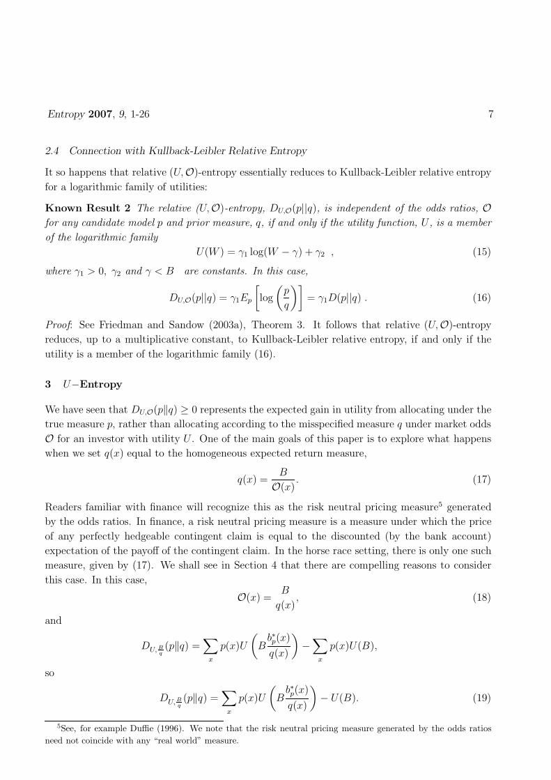
2.4 Connection with Kullback-Leibler Relative Entropy
It so happens that relative (U,O)-entropy essentially reduces to Kullback-Leibler relative entropy
for a logarithmic family of utilities:
Known Result 2 The relative (U,O)-entropy, DU,O(p||q), is independent of the odds ratios, O
for any candidate model p and prior measure, q, if and only if the utility function, U , is a member
of the logarithmic family
U(W ) = γ1 log(W − γ) + γ2 , (15)
where γ1 > 0, γ2 and γ < B are constants. In this case,
DU,O(p||q) = γ1Ep
[
log
(
p
q
)]
= γ1D(p||q) . (16)
Proof: See Friedman and Sandow (2003a), Theorem 3. It follows that relative (U,O)-entropy
reduces, up to a multiplicative constant, to Kullback-Leibler relative entropy, if and only if the
utility is a member of the logarithmic family (16).
3 U−Entropy
We have seen that DU,O(p‖q) ≥ 0 represents the expected gain in utility from allocating under the
true measure p, rather than allocating according to the misspecified measure q under market odds
O for an investor with utility U . One of the main goals of this paper is to explore what happens
when we set q(x) equal to the homogeneous expected return measure,
q(x) =B
O(x). (17)
Readers familiar with finance will recognize this as the risk neutral pricing measure5 generated
by the odds ratios. In finance, a risk neutral pricing measure is a measure under which the price
of any perfectly hedgeable contingent claim is equal to the discounted (by the bank account)
expectation of the payoff of the contingent claim. In the horse race setting, there is only one such
measure, given by (17). We shall see in Section 4 that there are compelling reasons to consider
this case. In this case,
O(x) =B
q(x), (18)
and
DU, Bq(p‖q) =
∑
x
p(x)U
(
Bb∗p(x)
q(x)
)
−∑
x
p(x)U(B),
so
DU, Bq(p‖q) =
∑
x
p(x)U
(
Bb∗p(x)
q(x)
)
− U(B). (19)
5See, for example Duffie (1996). We note that the risk neutral pricing measure generated by the odds ratios
need not coincide with any “real world” measure.
Entropy 2007, 9, 1-26 8
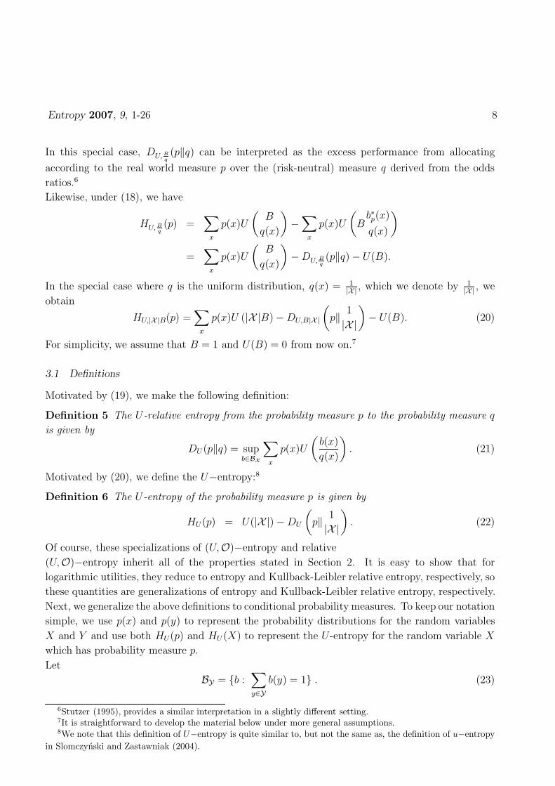
In this special case, DU, Bq(p‖q) can be interpreted as the excess performance from allocating
according to the real world measure p over the (risk-neutral) measure q derived from the odds
ratios.6
Likewise, under (18), we have
HU, Bq(p) =
∑
x
p(x)U
(
B
q(x)
)
−∑
x
p(x)U
(
Bb∗p(x)
q(x)
)
=∑
x
p(x)U
(
B
q(x)
)
− DU, Bq(p‖q) − U(B).
In the special case where q is the uniform distribution, q(x) = 1|X |
, which we denote by 1|X |
, we
obtain
HU,|X |B(p) =∑
x
p(x)U (|X |B)− DU,B|X |
(
p‖1
|X |
)
− U(B). (20)
For simplicity, we assume that B = 1 and U(B) = 0 from now on.7
3.1 Definitions
Motivated by (19), we make the following definition:
Definition 5 The U-relative entropy from the probability measure p to the probability measure q
is given by
DU (p‖q) = supb∈BX
∑
x
p(x)U
(
b(x)
q(x)
)
. (21)
Motivated by (20), we define the U−entropy:8
Definition 6 The U-entropy of the probability measure p is given by
HU (p) = U(|X |) − DU
(
p‖1
|X |
)
. (22)
Of course, these specializations of (U,O)−entropy and relative
(U,O)−entropy inherit all of the properties stated in Section 2. It is easy to show that for
logarithmic utilities, they reduce to entropy and Kullback-Leibler relative entropy, respectively, so
these quantities are generalizations of entropy and Kullback-Leibler relative entropy, respectively.
Next, we generalize the above definitions to conditional probability measures. To keep our notation
simple, we use p(x) and p(y) to represent the probability distributions for the random variables
X and Y and use both HU(p) and HU (X) to represent the U -entropy for the random variable X
which has probability measure p.
Let
BY = {b :∑
y∈Y
b(y) = 1} . (23)
6Stutzer (1995), provides a similar interpretation in a slightly different setting.7It is straightforward to develop the material below under more general assumptions.8We note that this definition of U−entropy is quite similar to, but not the same as, the definition of u−entropy
in Slomczynski and Zastawniak (2004).
Entropy 2007, 9, 1-26 9
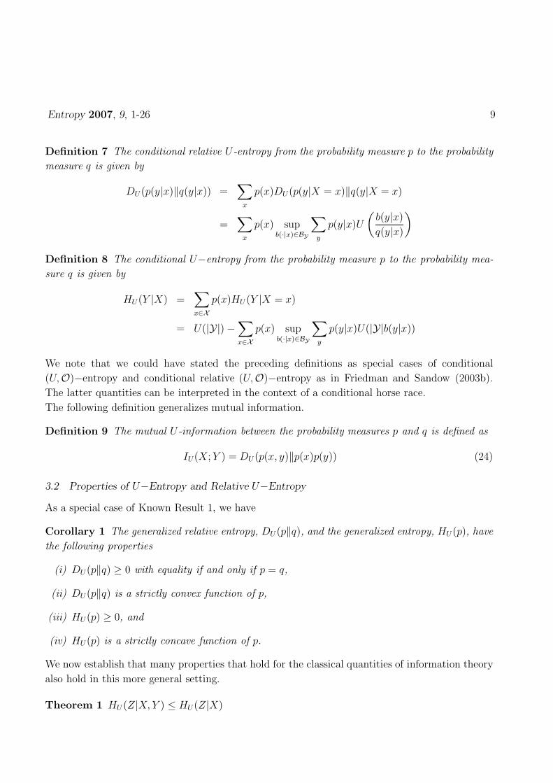
Definition 7 The conditional relative U-entropy from the probability measure p to the probability
measure q is given by
DU (p(y|x)‖q(y|x)) =∑
x
p(x)DU (p(y|X = x)‖q(y|X = x)
=∑
x
p(x) supb(·|x)∈BY
∑
y
p(y|x)U
(
b(y|x)
q(y|x)
)
Definition 8 The conditional U−entropy from the probability measure p to the probability mea-
sure q is given by
HU (Y |X) =∑
x∈X
p(x)HU (Y |X = x)
= U(|Y|) −∑
x∈X
p(x) supb(·|x)∈BY
∑
y
p(y|x)U(|Y|b(y|x))
We note that we could have stated the preceding definitions as special cases of conditional
(U,O)−entropy and conditional relative (U,O)−entropy as in Friedman and Sandow (2003b).
The latter quantities can be interpreted in the context of a conditional horse race.
The following definition generalizes mutual information.
Definition 9 The mutual U-information between the probability measures p and q is defined as
IU(X;Y ) = DU (p(x, y)‖p(x)p(y)) (24)
3.2 Properties of U−Entropy and Relative U−Entropy
As a special case of Known Result 1, we have
Corollary 1 The generalized relative entropy, DU (p‖q), and the generalized entropy, HU (p), have
the following properties
(i) DU (p‖q) ≥ 0 with equality if and only if p = q,
(ii) DU (p‖q) is a strictly convex function of p,
(iii) HU (p) ≥ 0, and
(iv) HU (p) is a strictly concave function of p.
We now establish that many properties that hold for the classical quantities of information theory
also hold in this more general setting.
Theorem 1 HU (Z|X,Y ) ≤ HU (Z|X)
Entropy 2007, 9, 1-26 10
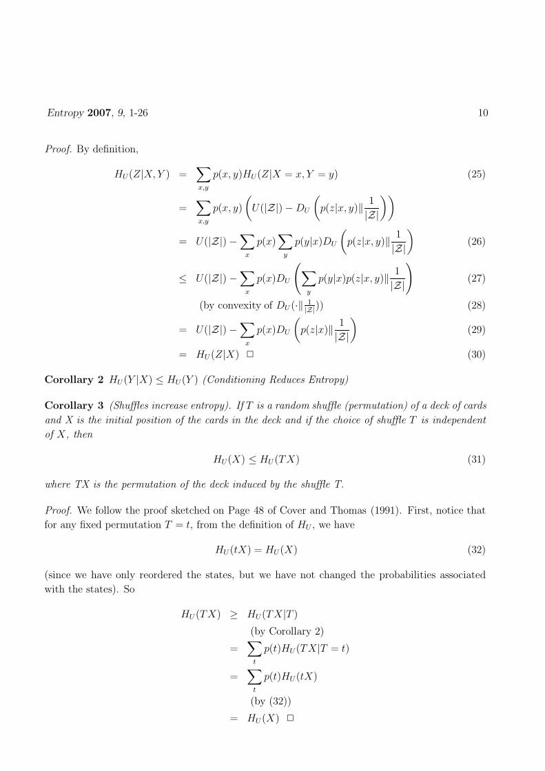
Proof. By definition,
HU(Z|X,Y ) =∑
x,y
p(x, y)HU(Z|X = x, Y = y) (25)
=∑
x,y
p(x, y)
(
U(|Z|) − DU
(
p(z|x, y)‖1
|Z|
))
= U(|Z|) −∑
x
p(x)∑
y
p(y|x)DU
(
p(z|x, y)‖1
|Z|
)
(26)
≤ U(|Z|) −∑
x
p(x)DU
(
∑
y
p(y|x)p(z|x, y)‖1
|Z|
)
(27)
(by convexity of DU (·‖ 1|Z|
)) (28)
= U(|Z|) −∑
x
p(x)DU
(
p(z|x)‖1
|Z|
)
(29)
= HU (Z|X) 2 (30)
Corollary 2 HU (Y |X) ≤ HU (Y ) (Conditioning Reduces Entropy)
Corollary 3 (Shuffles increase entropy). If T is a random shuffle (permutation) of a deck of cards
and X is the initial position of the cards in the deck and if the choice of shuffle T is independent
of X, then
HU(X) ≤ HU (TX) (31)
where TX is the permutation of the deck induced by the shuffle T.
Proof. We follow the proof sketched on Page 48 of Cover and Thomas (1991). First, notice that
for any fixed permutation T = t, from the definition of HU , we have
HU (tX) = HU (X) (32)
(since we have only reordered the states, but we have not changed the probabilities associated
with the states). So
HU (TX) ≥ HU (TX|T )
(by Corollary 2)
=∑
t
p(t)HU (TX|T = t)
=∑
t
p(t)HU (tX)
(by (32))
= HU (X) 2
Entropy 2007, 9, 1-26 11
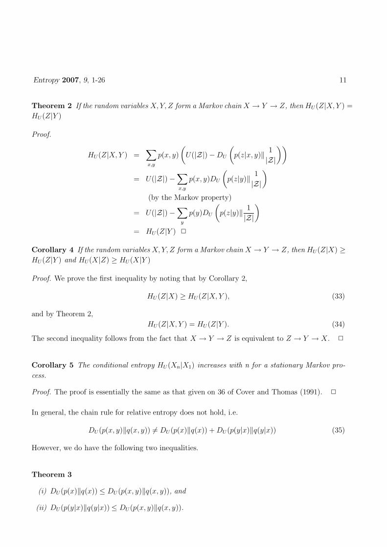
Theorem 2 If the random variables X,Y,Z form a Markov chain X → Y → Z, then HU (Z|X,Y ) =
HU (Z|Y )
Proof.
HU (Z|X,Y ) =∑
x,y
p(x, y)
(
U(|Z|) −DU
(
p(z|x, y)‖1
|Z|
))
= U(|Z|) −∑
x,y
p(x, y)DU
(
p(z|y)‖1
|Z|
)
(by the Markov property)
= U(|Z|) −∑
y
p(y)DU
(
p(z|y)‖1
|Z|
)
= HU (Z|Y ) 2
Corollary 4 If the random variables X,Y,Z form a Markov chain X → Y → Z, then HU (Z|X) ≥
HU (Z|Y ) and HU(X|Z) ≥ HU (X|Y )
Proof. We prove the first inequality by noting that by Corollary 2,
HU (Z|X) ≥ HU (Z|X,Y ), (33)
and by Theorem 2,
HU (Z|X,Y ) = HU (Z|Y ). (34)
The second inequality follows from the fact that X → Y → Z is equivalent to Z → Y → X. 2
Corollary 5 The conditional entropy HU (Xn|X1) increases with n for a stationary Markov pro-
cess.
Proof. The proof is essentially the same as that given on 36 of Cover and Thomas (1991). 2
In general, the chain rule for relative entropy does not hold, i.e.
DU (p(x, y)‖q(x, y)) 6= DU (p(x)‖q(x)) + DU (p(y|x)‖q(y|x)) (35)
However, we do have the following two inequalities.
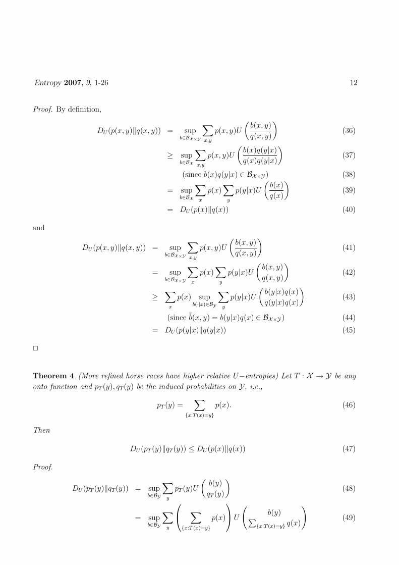
Theorem 3
(i) DU (p(x)‖q(x)) ≤ DU (p(x, y)‖q(x, y)), and
(ii) DU (p(y|x)‖q(y|x)) ≤ DU (p(x, y)‖q(x, y)).
Entropy 2007, 9, 1-26 12
Proof. By definition,
DU (p(x, y)‖q(x, y)) = supb∈BX×Y
∑
x,y
p(x, y)U
(
b(x, y)
q(x, y)
)
(36)
≥ supb∈BX
∑
x,y
p(x, y)U
(
b(x)q(y|x)
q(x)q(y|x)
)
(37)
(since b(x)q(y|x) ∈ BX×Y ) (38)
= supb∈BX
∑
x
p(x)∑
y
p(y|x)U
(
b(x)
q(x)
)
(39)
= DU (p(x)‖q(x)) (40)
and
DU (p(x, y)‖q(x, y)) = supb∈BX×Y
∑
x,y
p(x, y)U
(
b(x, y)
q(x, y)
)
(41)
= supb∈BX×Y
∑
x
p(x)∑
y
p(y|x)U
(
b(x, y)
q(x, y)
)
(42)
≥∑
x
p(x) supb(·|x)∈BY
∑
y
p(y|x)U
(
b(y|x)q(x)
q(y|x)q(x)
)
(43)
(since b(x, y) = b(y|x)q(x) ∈ BX×Y ) (44)
= DU (p(y|x)‖q(y|x)) (45)
2
Theorem 4 (More refined horse races have higher relative U−entropies) Let T : X → Y be any
onto function and pT (y), qT(y) be the induced probabilities on Y, i.e.,
pT (y) =∑
{x:T (x)=y}
p(x). (46)
Then
DU (pT (y)‖qT(y)) ≤ DU (p(x)‖q(x)) (47)
Proof.
DU (pT (y)‖qT(y)) = supb∈BY
∑
y
pT (y)U
(
b(y)
qT (y)
)
(48)
= supb∈BY
∑
y
∑
{x:T (x)=y}
p(x)
U
(
b(y)∑
{x:T (x)=y} q(x)
)
(49)
Entropy 2007, 9, 1-26 13
Define b(x) = q(x)b(T (x))∑{x′:T (x′)=T (x)} q(x′)
Then b(x) ∈ BX and
∑
y
∑
{x:T (x)=y}
p(x)
U
(
b(y)∑
{x:T (x)=y} q(x)
)
=∑
x
p(x)U
(
b(x)
q(x)
)
(50)
≤ DU (p(x)‖q(x)) (51)
2
Theorem 4 can also be regarded as a special case of Theorem 3, part (i).
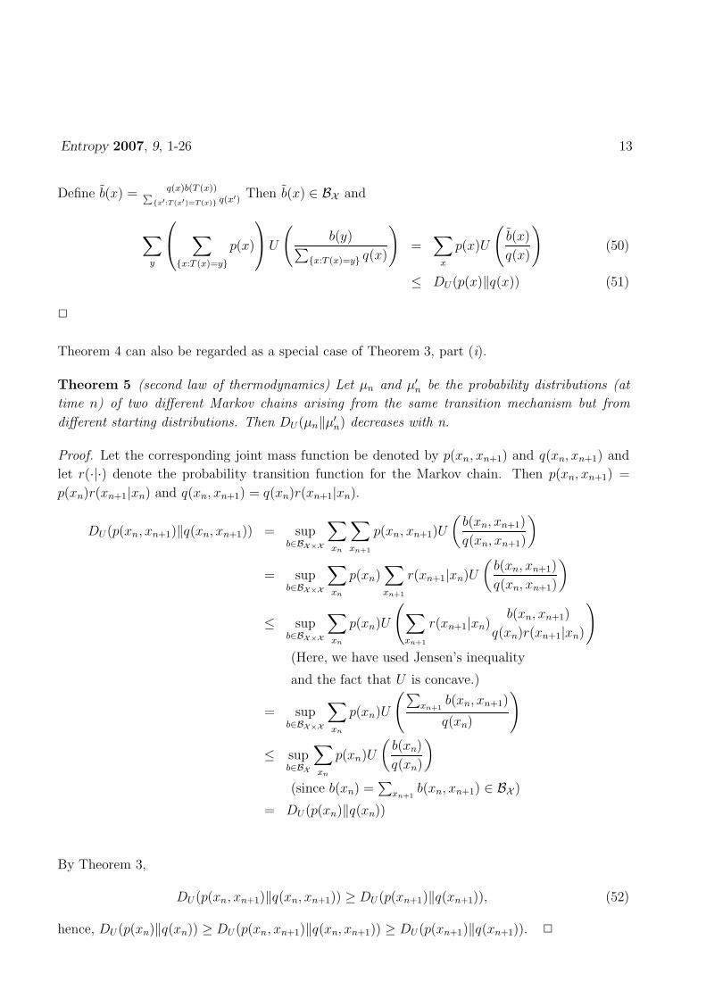
Theorem 5 (second law of thermodynamics) Let µn and µ′n be the probability distributions (at
time n) of two different Markov chains arising from the same transition mechanism but from
different starting distributions. Then DU (µn‖µ′n) decreases with n.
Proof. Let the corresponding joint mass function be denoted by p(xn, xn+1) and q(xn, xn+1) and
let r(·|·) denote the probability transition function for the Markov chain. Then p(xn, xn+1) =
p(xn)r(xn+1|xn) and q(xn, xn+1) = q(xn)r(xn+1|xn).
DU (p(xn, xn+1)‖q(xn, xn+1)) = supb∈BX×X
∑
xn
∑
xn+1
p(xn, xn+1)U
(
b(xn, xn+1)
q(xn, xn+1)
)
= supb∈BX×X
∑
xn
p(xn)∑
xn+1
r(xn+1|xn)U
(
b(xn, xn+1)
q(xn, xn+1)
)
≤ supb∈BX×X
∑
xn
p(xn)U
(
∑
xn+1
r(xn+1|xn)b(xn, xn+1)
q(xn)r(xn+1|xn)
)
(Here, we have used Jensen’s inequality
and the fact that U is concave.)
= supb∈BX×X
∑
xn
p(xn)U
(∑
xn+1b(xn, xn+1)
q(xn)
)
≤ supb∈BX
∑
xn
p(xn)U
(
b(xn)
q(xn)
)
(since b(xn) =∑
xn+1b(xn, xn+1) ∈ BX )
= DU (p(xn)‖q(xn))
By Theorem 3,
DU (p(xn, xn+1)‖q(xn, xn+1)) ≥ DU (p(xn+1)‖q(xn+1)), (52)
hence, DU (p(xn)‖q(xn)) ≥ DU (p(xn, xn+1)‖q(xn, xn+1)) ≥ DU (p(xn+1)‖q(xn+1)). 2
Entropy 2007, 9, 1-26 14
Corollary 6 The relative U-entropy DU (µn‖µ) between a distribution µn on the states at time n
and a stationary distribution µ decreases with n.
Proof: This is a special case of Theorem 5, where µ′n = µ for any n. 2
Corollary 7 If the uniform distribution 1|X |
is a stationary distribution, then entropy HU (µn)
increases with n.
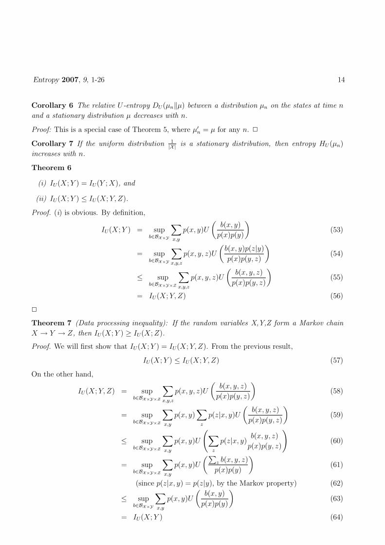
Theorem 6
(i) IU(X;Y ) = IU(Y ;X), and
(ii) IU(X;Y ) ≤ IU(X;Y,Z).
Proof. (i) is obvious. By definition,
IU(X;Y ) = supb∈BX×Y
∑
x,y
p(x, y)U
(
b(x, y)
p(x)p(y)
)
(53)
= supb∈BX×Y
∑
x,y,z
p(x, y, z)U
(
b(x, y)p(z|y)
p(x)p(y, z)
)
(54)
≤ supb∈BX×Y×Z
∑
x,y,z
p(x, y, z)U
(
b(x, y, z)
p(x)p(y, z)
)
(55)
= IU(X;Y,Z) (56)
2
Theorem 7 (Data processing inequality): If the random variables X,Y,Z form a Markov chain
X → Y → Z, then IU(X;Y ) ≥ IU(X;Z).
Proof. We will first show that IU(X;Y ) = IU(X;Y,Z). From the previous result,
IU(X;Y ) ≤ IU(X;Y,Z) (57)
On the other hand,
IU(X;Y,Z) = supb∈BX×Y×Z
∑
x,y,z
p(x, y, z)U
(
b(x, y, z)
p(x)p(y, z)
)
(58)
= supb∈BX×Y×Z
∑
x,y
p(x, y)∑
z
p(z|x, y)U
(
b(x, y, z)
p(x)p(y, z)
)
(59)
≤ supb∈BX×Y×Z
∑
x,y
p(x, y)U
(
∑
z
p(z|x, y)b(x, y, z)
p(x)p(y, z)
)
(60)
= supb∈BX×Y×Z
∑
x,y
p(x, y)U
(∑
z b(x, y, z)
p(x)p(y)
)
(61)
(since p(z|x, y) = p(z|y), by the Markov property) (62)
≤ supb∈BX×Y
∑
x,y
p(x, y)U
(
b(x, y)
p(x)p(y)
)
(63)
= IU(X;Y ) (64)
Entropy 2007, 9, 1-26 15
so IU(X;Y ) = IU(X;Y,Z) ≥ IU(X;Z). 2
Corollary 8 If Z = g(Y ), we have IU(X;Y ) ≥ IU(X; g(Y )).
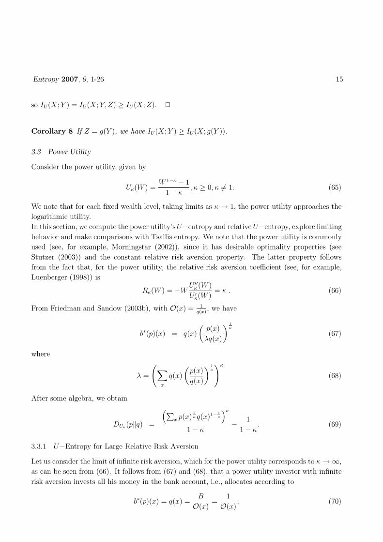
3.3 Power Utility
Consider the power utility, given by
Uκ(W ) =W 1−κ − 1
1 − κ, κ ≥ 0, κ 6= 1. (65)
We note that for each fixed wealth level, taking limits as κ → 1, the power utility approaches the
logarithmic utility.
In this section, we compute the power utility’s U−entropy and relative U−entropy, explore limiting
behavior and make comparisons with Tsallis entropy. We note that the power utility is commonly
used (see, for example, Morningstar (2002)), since it has desirable optimality properties (see
Stutzer (2003)) and the constant relative risk aversion property. The latter property follows
from the fact that, for the power utility, the relative risk aversion coefficient (see, for example,
Luenberger (1998)) is
Rκ(W ) = −WU ′′
κ (W )
U ′κ(W )
= κ . (66)
From Friedman and Sandow (2003b), with O(x) = 1q(x)
, we have
b∗(p)(x) = q(x)
(
p(x)
λq(x)
)1κ
(67)
where
λ =
(
∑
x
q(x)
(
p(x)
q(x)
) 1κ
)κ
(68)
After some algebra, we obtain
DUκ(p‖q) =
(
∑
x p(x)1κ q(x)1− 1
κ
)κ
1 − κ−
1
1 − κ. (69)
3.3.1 U−Entropy for Large Relative Risk Aversion
Let us consider the limit of infinite risk aversion, which for the power utility corresponds to κ → ∞,
as can be seen from (66). It follows from (67) and (68), that a power utility investor with infinite
risk aversion invests all his money in the bank account, i.e., allocates according to
b∗(p)(x) = q(x) =B
O(x)=
1
O(x), (70)
Entropy 2007, 9, 1-26 16
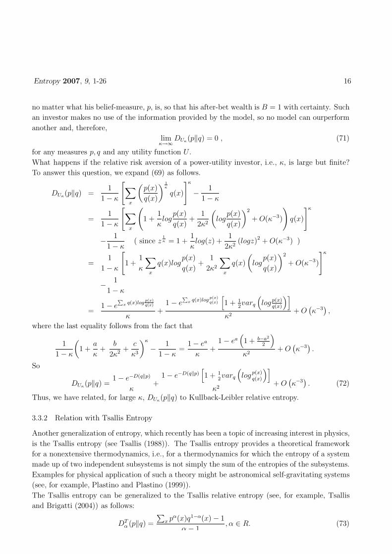
no matter what his belief-measure, p, is, so that his after-bet wealth is B = 1 with certainty. Such
an investor makes no use of the information provided by the model, so no model can ourperform
another and, therefore,
limκ→∞
DUκ(p‖q) = 0 , (71)
for any measures p, q and any utility function U .
What happens if the relative risk aversion of a power-utility investor, i.e., κ, is large but finite?
To answer this question, we expand (69) as follows.
DUκ(p‖q) =1
1 − κ
[
∑
x
(
p(x)
q(x)
) 1κ
q(x)
]κ
−1
1 − κ
=1
1 − κ
[
∑
x
(
1 +1
κlog
p(x)
q(x)+
1
2κ2
(
logp(x)
q(x)
)2
+ O(κ−3)
)
q(x)
]κ
−1
1 − κ( since z
1κ = 1 +
1
κlog(z) +
1
2κ2(logz)2 + O(κ−3) )
=1
1 − κ
[
1 +1
κ
∑
x
q(x)logp(x)
q(x)+
1
2κ2
∑
x
q(x)
(
logp(x)
q(x)
)2
+ O(κ−3)
]κ
−1
1 − κ
=1 − e
∑x q(x)log
p(x)q(x)
κ+
1 − e∑
x q(x)logp(x)q(x)
[
1 + 12varq
(
logp(x)q(x)
)]
κ2+ O
(
κ−3)
,
where the last equality follows from the fact that
1
1 − κ
(
1 +a
κ+
b
2κ2 +c
κ3
)κ
−1
1 − κ=
1 − ea
κ+
1 − ea(
1 + b−a2
2
)
κ2+ O
(
κ−3)
.
So
DUκ(p‖q) =1 − e−D(q‖p)
κ+
1 − e−D(q‖p)[
1 + 12varq
(
logp(x)q(x)
)]
κ2+ O
(
κ−3)
. (72)
Thus, we have related, for large κ, DUκ(p‖q) to Kullback-Leibler relative entropy.
3.3.2 Relation with Tsallis Entropy
Another generalization of entropy, which recently has been a topic of increasing interest in physics,
is the Tsallis entropy (see Tsallis (1988)). The Tsallis entropy provides a theoretical framework
for a nonextensive thermodynamics, i.e., for a thermodynamics for which the entropy of a system
made up of two independent subsystems is not simply the sum of the entropies of the subsystems.
Examples for physical application of such a theory might be astronomical self-gravitating systems
(see, for example, Plastino and Plastino (1999)).
The Tsallis entropy can be generalized to the Tsallis relative entropy (see, for example, Tsallis
and Brigatti (2004)) as follows:
DTα (p‖q) =
∑
x pα(x)q1−α(x) − 1
α − 1, α ∈ R. (73)
Entropy 2007, 9, 1-26 17
This entropy recovers the standard Boltzmann-Gibbs entropy α → 1. It turns out that there is a
simple monotonic relationship between our relative U−entropy and the relative Tsallis entropies:
DUκ(p‖q) =
(
DT1κ
(p‖q)(
1κ− 1)
+ 1)κ
− 1
1 − κ. (74)
Also note that
HUκ(X) = Uκ(|X |)− DUκ
(
p‖1
|X |
)
=|X |1−κ
[
1 −(
∑
x p(x)1κ
)κ]
1 − κ. (75)
Comparing this to the Tsallis entropy:
HTα (X) =
∑
x pα(x) − 1
1 − α; (76)
we have the following simple monotonic relationship between the two entropies
HUκ(X) =
[
1 −(
HT1κ
(X)(1 − 1κ) + 1
)κ]
|X |1−κ
1 − κ. (77)
4 Application: Probability Estimation via Relative U−Entropy Minimization
Information theoretic ideas such as the maximum entropy principle (see, for example, Jaynes
(1957) and Golan et al. (1996)) or the closely related minimum relative entropy (MRE) principle
(see, for example Lebanon and Lafferty (2001)) have assumed major roles in statistical learning.
We discuss these principles from the point of view of a model user who would use a probabilistic
model to make bets in the horse race setting of Section 2.9 As we shall see, probability models
estimated by these principles are robust in the sense that they maximize “worst case” model
performance, in terms of expected utility, for a horse race investor with the three parameter
logarithmic utility (15) in a particular market (horse race).
As such, probability models estimated by MRE methods are special in the sense that they are
tailored to the risk preferences of logarithmic-family-utility investors. However, not all risk prefer-
ences can be expressed by utility functions in the logarithmic family. In the financial community,
a substantial percentage, if not a majority, of practitioners implement utility functions outside
the logarithmic family (15) (see, for example, Morningstar (2002)). This is not surprising – other
utility functions may more accurately reflect the risk preferences of certain investors, or possess
important defining properties or optimality properties.
In order to tailor the statistical learning problem to the specific utility function of the investor,
one can replace the usual MRE problem with a generalization, based on relative U -entropy, as
indicated below. Before stating results for minimum relative U−entropy (MRUE) probability
estimation, we review results for MRE probability estimation.
9It is possible to consider more general settings, such as incomplete markets, but a number of results depend in
a fundamental way on the horse race setting.
Entropy 2007, 9, 1-26 18
4.1 MRE and Dual Formulation
The usual MRE formulation (see, for example, Lebanon and Lafferty (2001) and Kitamura and
Stutzer (1997)) is given by:10
Problem 1 Find
p∗ = arg minp∈Q
D(p||p0) (78)
s.t. Ep[fj] − Ep[f
j] = 0 , j = 1, . . . , J , (79)
where each f j represents a feature (i.e., a function that maps X to R), p0 is a probability measure,
p represents the empirical measure, and Q is the set of all probability measures.
The feature constraints (79) can be viewed as a mechanism to enforce ”consistency” between the
model and the data. Typically, p0 is interpreted as representing prior beliefs, before modification
in light of model training data. Below, we discuss what happens when p0 is a benchmark measure
or the pricing measure generated by the odds ratios. The solution to Problem 1 will be the measure
satisfying the feature constraints that is closest to p0 (in the sense of relative entropy).
In many settings, the above (primal) problem is not as easy to solve numerically as the following
dual problem:11
Problem 2 Find
β∗ = arg maxβ∈RJ
L(pβ) , (80)
where L(p) =∑
x
p(x) log(p(x)) (81)
is the log-likelihood function,
pβ(x) =1
Zp0(x)eβT f(x) (82)
and Z =∑
x
p0(x)eβT f(x) , (83)
and p(x) denotes the empirical probability that X = x.
We note that the primal problem (Problem 1) and the dual problem (Problem 2) have the same
solution, in the sense that p∗ = pβ∗.
10MRE problems can be stated for conditional probability estimation and with regularization. We keep the
context and notation as simple as possible by confining our discussion to unconditional estimation without regu-
larization. Extensions are straightforward.11See, for example, Lebanon and Lafferty (2001).
Entropy 2007, 9, 1-26 19
4.2 Robustness of MRE when the Prior Measure is the Odds Ratio Pricing Measure
In a certain circumstance, the MRE measure (i.e., the solution of Problem 1) has a desirable
robustness property, which we discuss in this section. First we state the following minimax result
from Grunwald and Dawid (2004).
Known Result 3 If there exists a probability measure π ∈ K, with πx > 0,∀x ∈ X , then
infp′∈K
(−H(p′)) = infp∈K
supp′∈Q
Ep [log p′] = supp′∈Q
infp∈K
Ep [log p′] , (84)
where Q is the set of all possible probability measures, K is a closed convex set, such as the set of
all p ∈ Q that satisfy the feature constraints, (79). Moreover, a saddle point is attained.
Replacing log p′ with log p′− log p0 in (84) doesn’t change the finiteness or the convexity properties
of the function under the infsup or the supinf. Since the proof of Known Result 3 relies only on
those properties of this function, we have
infp∈K
supp′∈Q
Ep
[
log p′ − log p0]
= supp′∈Q
infp∈K
Ep
[
log p′ − log p0]
, (85)
and a saddle point is attained here as well. Further using the fact that
D(p||p0) = supp′∈Q
Ep
[
log p′ − log p0]
, (86)
which follows from the information inequality (see, for example, Cover and Thomas (1991)), we
obtain
infp∈K
D(p||p0) = supp′∈Q
infp∈K
Ep
[
log p′ − log p0]
= supp∈Q
infp′∈K
Ep′
[
log p − log p0]
. (87)
Using further b∗(p) = p,12 for U(W ) = log W , we see that (87) leads to the following corollary:
Corollary 9 If U(W ) = log W , and
p0(x) =B
O(x)=
1
O(x),∀x ∈ X , (88)
then
p∗ = arg minp∈K
D(p||p0) = arg maxp∈Q
minp′∈K
Ep′[U(b∗(p),O)], (89)
where Q is the set of all possible probability measures and K is the set of all p ∈ Q that satisfy
the feature constraints, (79).13
12See, for example, Cover and Thomas (1991), Theorem 6.1.2.13For ease of exposition, we have proved this result for U (·) = log(·). The same result holds for utilities in the
generalized logarithmic family (15).
Entropy 2007, 9, 1-26 20
Thus, if p0 is given by pricing measure generated by the odds ratios, then the MRE measure, p∗,
is robust in the following sense: by choosing p∗ a rational (expected-utility optimizing) investor
maximizes his (model-based optimal) expected utility in the most adverse environment consistent
with the feature constraints.
Here, p0 has a specific and non-traditional interpretation. It no longer represents prior beliefs about
the real world measure that we estimate with p∗. Rather, it represents the risk neutral pricing
measure consistent with the odds ratios. If a logarithmic utility investor wants the measure that
he estimates to have the optimality property (89), he is not free to choose p0 to represent his prior
beliefs, in general. However, if he sets p0 to the risk neutral pricing measure determined by the
odds ratios, then the optimality property (89) will hold. In this case, p∗, can be thought of as a
function of the odds ratios, rather than an update of prior beliefs.
It is this property, (89), that we seek to generalize to accommodate risk preferences more general
than the ones compatible with a logarithmic utility function.
4.3 General Risk Preferences and Robust Relative Performance
In this section, we state a known result that we will use below to generalize the robustness property
(89).
The MRE problem is generalized in Friedman and Sandow (2003a) to a minimum relative (U,O)
entropy problem. The solution to this generalized problem is robust in the following sense:
Known Result 4
arg minp∈K
DU,O(p||p0) = arg maxp∈Q
minp′∈K
{
Ep′ [U(b∗(p),O)] − Ep′
[
U(b∗(p0),O)]}
,
where Q is the set of all possible probability measures, K is the set of all p ∈ Q that satisfy the
feature constraints, (79).
This is only a slight modification of a result from Grunwald and Dawid (2002) and is based on
the logic from Topsøe (1979). A proof can be found in Friedman and Sandow (2003a).
Known Result 4 states the following: minimizing DU,O(p||p0) with respect to p ∈ K is equivalent
to searching for the measure p∗ ∈ Q that maximizes the worst-case (with respect to the potential
true measures, p′ ∈ K) relative model performance (over the benchmark model, p0), in the sense
of expected utility. The optimal model, p∗, is robust in the sense that for any other model, p, the
worst (over potential true measures p′ ∈ K) relative performance is even worse than the worst-
case relative performance under p∗. We do not know the true measure; an investor who makes
allocation decisions based on p∗ is prepared for the worst that “nature” can offer.
4.4 Robust Absolute Performance and MRUE
We now address the following question: Is it possible to formulate a generalized MRE problem
for which the solution is robust in the absolute sense of (89), as opposed to the relative sense in
Known Result 4? This is indeed possible, as the following Corollary, which follows directly from
Known Result 4, indicates:
Entropy 2007, 9, 1-26 21
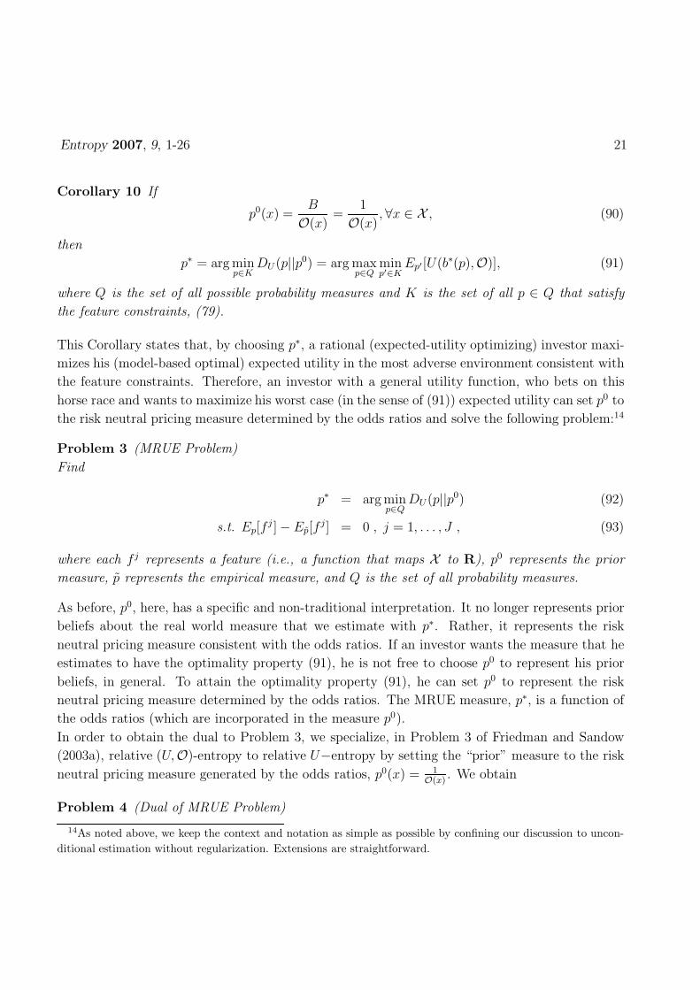
Corollary 10 If
p0(x) =B
O(x)=
1
O(x),∀x ∈ X , (90)
then
p∗ = arg minp∈K
DU (p||p0) = arg maxp∈Q
minp′∈K
Ep′[U(b∗(p),O)], (91)
where Q is the set of all possible probability measures and K is the set of all p ∈ Q that satisfy
the feature constraints, (79).
This Corollary states that, by choosing p∗, a rational (expected-utility optimizing) investor maxi-
mizes his (model-based optimal) expected utility in the most adverse environment consistent with
the feature constraints. Therefore, an investor with a general utility function, who bets on this
horse race and wants to maximize his worst case (in the sense of (91)) expected utility can set p0 to
the risk neutral pricing measure determined by the odds ratios and solve the following problem:14
Problem 3 (MRUE Problem)
Find
p∗ = arg minp∈Q
DU (p||p0) (92)
s.t. Ep[fj ]− Ep[f
j] = 0 , j = 1, . . . , J , (93)
where each f j represents a feature (i.e., a function that maps X to R), p0 represents the prior
measure, p represents the empirical measure, and Q is the set of all probability measures.
As before, p0, here, has a specific and non-traditional interpretation. It no longer represents prior
beliefs about the real world measure that we estimate with p∗. Rather, it represents the risk
neutral pricing measure consistent with the odds ratios. If an investor wants the measure that he
estimates to have the optimality property (91), he is not free to choose p0 to represent his prior
beliefs, in general. To attain the optimality property (91), he can set p0 to represent the risk
neutral pricing measure determined by the odds ratios. The MRUE measure, p∗, is a function of
the odds ratios (which are incorporated in the measure p0).
In order to obtain the dual to Problem 3, we specialize, in Problem 3 of Friedman and Sandow
(2003a), relative (U,O)-entropy to relative U−entropy by setting the “prior” measure to the risk
neutral pricing measure generated by the odds ratios, p0(x) = 1O(x)
. We obtain
Problem 4 (Dual of MRUE Problem)
14As noted above, we keep the context and notation as simple as possible by confining our discussion to uncon-
ditional estimation without regularization. Extensions are straightforward.
Entropy 2007, 9, 1-26 22
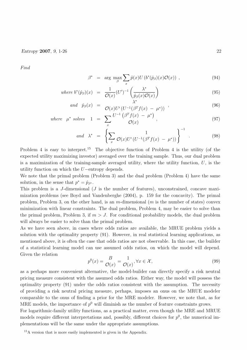
Find
β∗ = arg maxβ
∑
x
p(x)U (b∗(pβ)(x)O(x)) , (94)
where b∗(pβ)(x) =1
O(x)(U ′)−1
(
λ∗
pβ(x)O(x)
)
(95)
and pβ(x) =λ∗
O(x)U ′ (U−1(βTf(x) − µ∗)), (96)
where µ∗ solves 1 =∑
x
U−1(
βTf(x) − µ∗)
O(x), (97)
and λ∗ =
{
∑
x
1
O(x)U ′ (U−1(βTf(x) − µ∗))
}−1
. (98)
Problem 4 is easy to interpret.15 The objective function of Problem 4 is the utility (of the
expected utility maximizing investor) averaged over the training sample. Thus, our dual problem
is a maximization of the training-sample averaged utility, where the utility function, U , is the
utility function on which the U−entropy depends.
We note that the primal problem (Problem 3) and the dual problem (Problem 4) have the same
solution, in the sense that p∗ = pβ∗.
This problem is a J -dimensional (J is the number of features), unconstrained, concave maxi-
mization problems (see Boyd and Vandenberghe (2004), p. 159 for the concavity). The primal
problem, Problem 3, on the other hand, is an m-dimensional (m is the number of states) convex
minimization with linear constraints. The dual problem, Problem 4, may be easier to solve than
the primal problem, Problem 3, if m > J . For conditional probability models, the dual problem
will always be easier to solve than the primal problem.
As we have seen above, in cases where odds ratios are available, the MRUE problem yields a
solution with the optimality property (91). However, in real statistical learning applications, as
mentioned above, it is often the case that odds ratios are not observable. In this case, the builder
of a statistical learning model can use assumed odds ratios, on which the model will depend.
Given the relation
p0(x) =B
O(x)=
1
O(x),∀x ∈ X , (99)
as a perhaps more convenient alternative, the model-builder can directly specify a risk neutral
pricing measure consistent with the assumed odds ratios. Either way, the model will possess the
optimality property (91) under the odds ratios consistent with the assumption. The necessity
of providing a risk neutral pricing measure, perhaps, imposes an onus on the MRUE modeler
comparable to the onus of finding a prior for the MRE modeler. However, we note that, as for
MRE models, the importance of p0 will diminish as the number of feature constraints grows.
For logarithmic-family utility functions, as a practical matter, even though the MRE and MRUE
models require different interpretations and, possibly, different choices for p0, the numerical im-
plementations will be the same under the appropriate assumptions.
15A version that is more easily implemented is given in the Appendix.
Entropy 2007, 9, 1-26 23
5 Conclusions
Motivated by decision theory, we have defined a generalization of entropy (U−entropy) and a
generalization of relative entropy (relative U−entropy). We have shown that these generaliza-
tions retain a number of properties of entropy and relative entropy that are not retained by the
generalizations DU,O and HU,O presented in Friedman and Sandow (2003a).
We have used relative U−entropy to formulate an approach to the probability measure estimation
problem (Problem 3). Problem 3 generalizes the absolute robustness properties of the solution to
the MRE problem, incorporating risk preferences more general than those that can be expressed
via the logarithmic family (15).
Depending on the situation, the model builder may prefer one of the methods listed below:
I General Risk Preferences (not expressible by (15)), real or assumed odds ratios available
(i) MRUE, Problem 3: If p0 is the pricing measure generated by the odds ratios, we get
robust absolute performance (in the market described by the odds ratios) in the sense
of Corollary 10.
(ii) Minimum Relative (U,O)−entropy Problem from Friedman and Sandow (2003a): If p0
represents a benchmark model (possibly prior beliefs), we get robust relative outperfor-
mance (relative to the benchmark model, in the market described by the odds ratios)
in the sense of Known Result 4.
II Special Case: Logarithmic Family Risk Preferences (15), odds ratios need not be available
MRE, Problem 1: If p0 represents a benchmark model (possibly prior beliefs), we get
robust relative outperformance with respect to the benchmark model, under any odds
ratios.
6 Appendix
If we specialize relative (U,O)-entropy to relative U−entropy, substituting
p0(x) =B
O(x)=
1
O(x),∀x ∈ X , (100)
in Problem 4 of Friedman and Sandow (2003a), we obtain a version of the dual problem that is
easier to implement, though the objective function is not as easy to interpret as the objective
function in Problem 4.
Problem 5 (Easily Implemented Version of Dual Problem)
Find β∗ = arg maxβ
{βTEp[f ] − µ∗} , (101)
(102)
where µ∗ solves 1 =∑
x
p0(x)U−1(
βTf(x) − µ∗)
. (103)
Entropy 2007, 9, 1-26 24
Once Problem 5 is solved, the solution to Problem 3 is simply,
p∗(x) = λ∗ p0(x)
U ′(
U−1(β∗T f(x) − µ∗)) (104)
where λ∗ is the positive constant that makes∑
x p∗(x) = 1.
References
S. Boyd and L. Vandenberghe. Convex Optimization. Cambridge, 2004.
L. Brillouin. Science and Information Theory. Academic Press, New York, 1962.
T. Cover and J. Thomas. Elements of Information Theory. Wiley, New York, 1991.
F. Cowell. Additivity and the entropy concept: An axiomatic approach to inequality measurement.
Journal of Economic Theory, 25:131–143, 1981.
N. Cressie and T. Read. Multinomial goodness of fit tests. journal of the royal statistical society
b, 46(3):440–464, 1984.
N. Cressie and T. Read. Pearson’s x2 and the loglikelihood ratio statistic g2: a comparative review.
International statistical review, 57(1):19–43, 1989.
I. Csiszar and J. Korner. Information theory: Coding Theorems for Discrete Memoryless Systems.
Academic Press, New York, 1997.
D. Duffie. Dynamic Asset Pricing Theory. Princeton University Press, Princeton, 1996.
C. Friedman and S. Sandow. Learning probabilistic models: An expected utility maximization
approach. Journal of Machine Learning Research, 4:291, 2003a.
C. Friedman and S. Sandow. Model performance measures for expected utility maximizing in-
vestors. International Journal of Theoretical and Applied Finance, 6(4):355, 2003b.
C. Friedman and S. Sandow. Model performance measures for leveraged investors. International
Journal of Theoretical and Applied Finance, 7(5):541, 2004.
A. Golan, G. Judge, and D. Miller. Maximum Entropy Econometrics. Wiley, New York, 1996.
Group of Statistical Physics. Nonextensive statistical mechanics and thermodynamics: Bibliogra-
phy. Working Paper, http://tsallis.cat.cbpf.br/TEMUCO.pdf, 2006.
P. Grunwald and A. Dawid. Game theory, maximum generalized entropy, minimum discrepancy,
robust bayes and pythagoras. Proceedings ITW, 2002.
P. Grunwald and A. Dawid. Game theory, maximum generalized entropy, minimum discrepancy,
and robust bayesian decision theory. Annals of Statistics, 32(4):1367–1433, 2004.
Entropy 2007, 9, 1-26 25
J. Ingersoll. Theory of Financial Decision Making. Rowman and Littlefield, New York, 1987.
E. T. Jaynes. Information theory and statistical mechanics. Physical Review, 106:620, 1957.
Y. Kitamura and M. Stutzer. An information-theoretic alternative to generalized method of
moments. Econometrica, 65(4):861–874, 1997.
G. Lebanon and J. Lafferty. Boosting and maximum likelihood for exponential models. Technical
Report CMU-CS-01-144 School of Computer Science Carnegie Mellon University, 2001.
F. Liese and I. Vajda. Convex Statistical Distances. Teubner, Leipzig, 1987.
D. Luenberger. Investment Science. Oxford University Press, New York, 1998.
Morningstar. The new morningstar ratingTM methodology.
http://www.morningstar.dk/downloads/MRARdefined.pdf, 2002.
F. Osterreicher and I. Vajda. Statistical information and discrimination. IEEE transactions on
information theory, 39(3):1036–1039, May, 1993.
A. Plastino and A. R. Plastino. Tsallis entropy and Jaynes’ informnation theory formalism.
Brazilian Journal of Physics, 29(1):50, 1999.
C. E. Shannon. A mathematical theory of communication. Bell System Technical Journal, 27:
379–423 and 623–656, Jul and Oct 1948.
W. Slomczynski and T. Zastawniak. Utility maximizing entropy and the second law of thermo-
dynamics. Annals of Probability, 32(3A):2261, 2004.
W. Stummer. On a statistical information measure of diffusion processes. statistics and decisions,
17:359–376, 1999.
W. Stummer. On a statistical information measure for a Samuelson-Black-Scholes model. statistics
and decisions, 19:289–313, 2001.
W. Stummer. Exponentials, Diffusions, Finance, Entropy and Information. Shaker, 2004.
M. Stutzer. A bayesian approach to diagnosis of asset pricing models. Journal of Econometrics,
68:367–397, 1995.
M. Stutzer. Portfolio choice with endogenous utility: A large deviations approach. Journal of
Econometrics, 116:365–386, 2003.
F. Topsøe. Information theoretical optimization techniques. Kybernetika, 15(1):8, 1979.
C. Tsallis. Possible generalization of Boltzmann-Gibbs statistics. Journal of Statistical Physics,
52:479, 1988.

Entropy 2007, 9, 1-26 26
C. Tsallis and E. Brigatti. Nonextensive statistical mechanics: A brief introduction. Continuum
Mechechanics and Thermodynanmics, 16:223–235, 2004.
c©2007 by MDPI (http://www.mdpi.org). Reproduction for noncommercial purposes permitted.