1

A Unifying Bayesian Optimization Framework forRadio Frequency Localization

Nachikethas A. Jagadeesan and Bhaskar Krishnamachari

Abstract—We consider the problem of estimating an RF-device’s location based on observations, such as received signalstrength, from a set of transmitters with known locations. Wesurvey the literature on this problem, showing that previousauthors have considered implicitly or explicitly various metrics.We present a Bayesian optimization framework that unifies theseworks and shows how to optimize the location estimation withrespect to a given metric. We demonstrate how the frameworkcan incorporate a general class of algorithms, including bothmodel-based methods and data-driven algorithms such finger-printing. This is illustrated by re-deriving the most popularalgorithms within this framework. Furthermore, we proposeusing the error-CDF as a unified way of comparing algorithmsbased on two methods: (i) stochastic dominance, and (ii) an upperbound on error-CDFs. We prove that an algorithm that optimizesany distance based cost function is not strictly stochasticallydominated by any other algorithm. This suggests that in lieuof the search for a universally best localization algorithm, thecommunity should focus on finding the best algorithm for a givenwell-defined objective.

Index Terms—Indoor environments, Algorithm design andanalysis, Estimation, Optimization, Bayes methods.

I . I N T R O D U C T I O N

THE ability to locate a wireless device based on receivedsignal strength from known-location transmitters is of

great utility for many applications, including indoor location-based mobile apps and services, interactive media, emergencysearch and rescue, asset tracking, etc. A significant numberof researchers have tackled this fundamental problem andproposed various algorithms for radio signal strength (RSS)based localization. Many works adopt standard algorithmsfrom signal processing, specifically estimation theory, such asMaximum Likelihood Estimation [1], Minimum Mean SquaredError Estimation [2], Best Linear Unbiased Estimator [3], etc.,while other techniques such as fingerprinting [4], and sequence-based localization [5], are somewhat more heuristically derived.These algorithms are typically evaluated using numerical andtrace-based simulations, using varied metrics such as the meansquared position error, the absolute distance error, etc.

We contend that the literature is disconnected and disorga-nized and that it is hard to decipher any unified theory that fairlyevaluates these algorithms across different metrics of interest.We argue that the state-of-the-art approach to localization inthe literature — which typically involves first presenting analgorithm and then evaluating its performance according to

The authors are with the Department of Electrical Engineering, Universityof Southern California, Los Angeles, CA 90089. Email: {nanantha,bkrishna}@usc.edu

a particular metric or a set of metrics — is akin to puttingthe proverbial cart before the horse. For instance, it is notuncommon for algorithms to be evaluated on metrics for whichthey are not explicitly or implicitly optimized.

We advocate a systematic way of designing location estima-tion algorithms which we refer to as the “optimization-basedapproach to localization”. In this approach, first the localizationmetric is defined in terms of a suitable cost function, thenan appropriate estimation algorithm is derived to minimizethat cost function. In addition, our optimization frameworkis applicable to any deterministic or stochastic model of theobservations (assumed to be known) and can accommodate anyprior distribution for location. Our framework also applies todata-driven approaches such as fingerprinting. We show that, insuch data-driven settings, our framework makes better use of theavailable data compared to traditional methods. Fundamentallya Bayesian approach, this framework is also compatible withBayesian filtering for location tracking over time [6].

As an illustration of our framework, we consider first a com-mon metric used in the evaluation of localization algorithms, theabsolute distance error, and derive an algorithm which yieldslocation estimates so as to minimize the expected distanceerror (MEDE). For a second illustration, we also consider asanother metric the probability that the location estimate iswithin a given radius of the true location (P(d)) and derivean algorithm which maximizes this probability. Furthermore,we show that standard algorithms such as MLE and MMSEcan be derived similarly from optimizing the correspondingmetrics (likelihood, mean squared error respectively).

In conjunction with our framework for deriving algorithmsto optimize a specified metric, we also consider the problemof comparing different localization algorithms with each other;for which we make use of the error CDF. For an importantclass of cost functions that can be expressed as non-negativemonotonically increasing functions of distance error, we provethat there is in effect a partial ordering among various estimationalgorithms. Certain algorithms dominate other algorithms forall such cost functions, and we show the necessary conditionfor this to happen. But there could also be two algorithms, A1and A2, and two metrics, M1 and M2, such that A1 is betterthan A2 in terms of M1 while the reverse is true for M2. Thuswe show that there is, in general, no single-best localizationalgorithm, but rather a “Pareto Set” of algorithms that are eachoptimized for different cost functions.

We evaluate the optimization-based framework for locationestimation using both numerical simulations, traces [7], anddata obtained from experiments in an indoor office environment.We illustrate how our framework can incorporate a variety of

2

localization algorithms, including fingerprinting based methods.Our evaluation confirms what is predicted by the theory — nosingle algorithm outperforms others with respect to all metrics,thus underlining the need for an optimization based approachsuch as the one we propose.

A. Contributions

• We describe an optimization-based Bayesian frameworkthat unifies and puts in context various previously proposedtechniques for localization and provides a systematic basisfor developing new algorithms.

• We introduce a partial ordering over the set of algorithmsby considering a stochastic dominance relationship be-tween their error CDFs. We prove that any algorithmthat optimizes a distance based cost function is notstochastically dominated by any other algorithm.

• We also present how algorithms may be compared basedon how ‘close’ an algorithm gets to the upper bound onerror CDFs. We propose one such measure of closeness(area of difference) and identify MEDE as the optimalalgorithm over that measure.

• We illustrate how our framework encompasses both model-based approaches and data-driven methods such as finger-printing, through simulations and real-world experiments.

The rest of the paper is organized as follows: A survey of theexisting literature on RSS based localization algorithms is givenin Section II. We introduce our optimization based localizationframework in Section III. In Section IV we introduce theconcept of stochastic dominance and prove how it leads toa partial ordering over the set of localization algorithms. Wealso introduce the upper bound on error CDFs and illustratethe evaluation of algorithms using the same. In Section V weevaluate our framework using simulations and trace data. Wealso show how fingerprinting methods fit into our framework.We conclude in Section VI.

I I . L I T E R AT U R E O N R S S B A S E D L O C A L I Z AT I O N

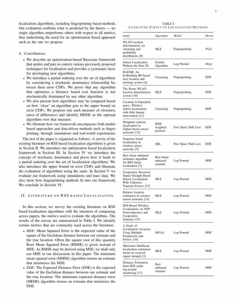
In this section, we survey the existing literature on RSSbased localization algorithms with the intention of comparing,across papers, the metrics used to evaluate the algorithms. Theresults of the survey are summarized in Table I. We identifycertain metrics that are commonly used across the literature:• MSE: Mean Squared Error is the expected value of the

square of the Euclidean distance between our estimate andthe true location. Often the square root of this quantityRoot Mean Squared Error (RMSE) is given instead ofMSE. As RMSE may be derived using MSE, we shall onlyuse MSE in our discussions in this paper. The minimummean squared error (MMSE) algorithm returns an estimatethat minimizes the MSE.

• EDE: The Expected Distance Error (EDE) is the expectedvalue of the Euclidean distance between our estimate andthe true location. The minimum expected distance error(MEDE) algorithm returns an estimate that minimizes theEDE.

TABLE IL I T E R AT U R E S U RV E Y O N L O C A L I Z AT I O N M E T H O D S

Study Algorithm Model Metric

WLAN locationdetermination viaclustering andprobabilitydistributions [8]

MLE Fingerprinting P(d)

Indoor LocalizationWithout the Pain [9]

GeneticAlgorithm Log-Normal D(p)

RADAR: AnIn-Building RF-baseduser location andtracking system [4]

Clustering Fingerprinting EDE

The Horus WLANlocation determinationsystem [10]

MLE Fingerprinting EDE

Locating in fingerprintspace: Wirelessindoor localizationwith little humanintervention [11]

Clustering Fingerprinting EDE

Weighted centroidlocalization inZigbee-based sensornetworks [12]

RSSIweightedposition

Free Space Path Loss EDE

Sequence basedlocalization inwireless sensornetworks [5]

SBL Free Space Path Loss EDE

Best linear unbiasedestimator algorithmfor RSS basedlocalization [3]

Best linearunbiasedestimate

Log-Normal MSE

Cooperative ReceivedSignal Strength-BasedSensor LocalizationWith UnknownTransmit Powers [13]

MLE Log-Normal MSE

Relative locationestimation in wirelesssensor networks [14]

MLE Log-Normal MSE

RSS-Based WirelessLocalization via SDP:Noncooperative andCooperativeSchemes [15]

MLE Log-Normal MSE

A Study ofLocalization AccuracyUsing MultipleFrequencies andPowers [16]

MP(d) Log-Normal MSE

Maximum likelihoodlocalization estimationbased on receivedsignal strength [1]

MLE Log-Normal MSE

Distance Estimationfrom RSS underlog-normalshadowing [17]

Bestunbiasedestimate

Log-Normal MSE

3

• P(d): P(d) indicates the probability that the receiverlocation is within a distance of d from our locationestimate. P(d) is closely related to the metric D(p) whichgives the radius at which an open ball around our locationestimate yields a probability of at least p. The MP(d)algorithm returns an estimate that minimizes the P(d).

As evidenced by Table I, it is with striking regularity that oneencounters a mismatch between an algorithm and the metricused for its evaluation. While there is hardly anything amissin checking how an algorithm performs on a metric that it isnot optimized for, it is shortsighted to draw a conclusion as tothe efficacy of the said algorithm based on such an evaluation.An awareness of the metric that an algorithm is implicitlyor explicitly optimized for, is essential to its fair assessment.We believe that such of notion of consistent evaluation ofalgorithms across all important metrics of interest has beenabsent in the community so far. In addition, while the literatureon localization abounds in algorithms that yield a locationestimate, there is no unifying theory that relates them to eachother with appropriate context.

For instance, [18] picks four algorithms for evaluation,independent of the metrics used to evaluate the algorithms. Suchan approach makes it unclear if an algorithm is optimal withrespect with any of the given metrics. In this case, we can onlymake (empirical) inferences regarding the relative ordering ofthe chosen algorithms among the chosen metrics. Consequently,there are no theoretical guarantees on algorithm performanceand it becomes hard, if not impossible, to accurately predicthow a chosen algorithm will behave when evaluated with ametric that was not considered.

Moreover, while error CDFs have been used earlier to eval-uate localization algorithms [16], [19]–[21], they are typicallyused to derive inferences about algorithm performance withrespect to the Euclidean distance and D(p) metrics. In theabsence of the unifying theory presented in this proposal, it isunclear how one may draw meaningful conclusions regardingthe relative performance of algorithms across various metricsbased on their error CDF. Our proposed unifying frameworkplaces the commonly employed subjective reading of errorCDFs on a firm theoretical footing and enables a better under-standing of algorithm performance than what was previouslypossible. Moreover, our framework is computationally tractableas the optimization is typically done over a reasonably sizeddiscrete set of possible locations.

Table I also indicates that there is considerable interest in thecommunity for the EDE metric. However, it is interesting tonote that none of the algorithms evaluated using that metric areexplicitly optimized for it. In the following sections we showhow such metrics fit into our framework. More importantly, itis our hope that thinking in terms of the framework below shalllead to a clearer understanding of the trade-offs involved inchoosing an algorithm and a better specification of the criterionnecessary for its adoption.

The optimization-based framework for localization presentedin this paper is inspired in part by the optimization-basedapproach to networking developed since the late 90’s [22],which has shown successfully that efficient medium access,routing, and congestion control algorithms, protocols, and archi-

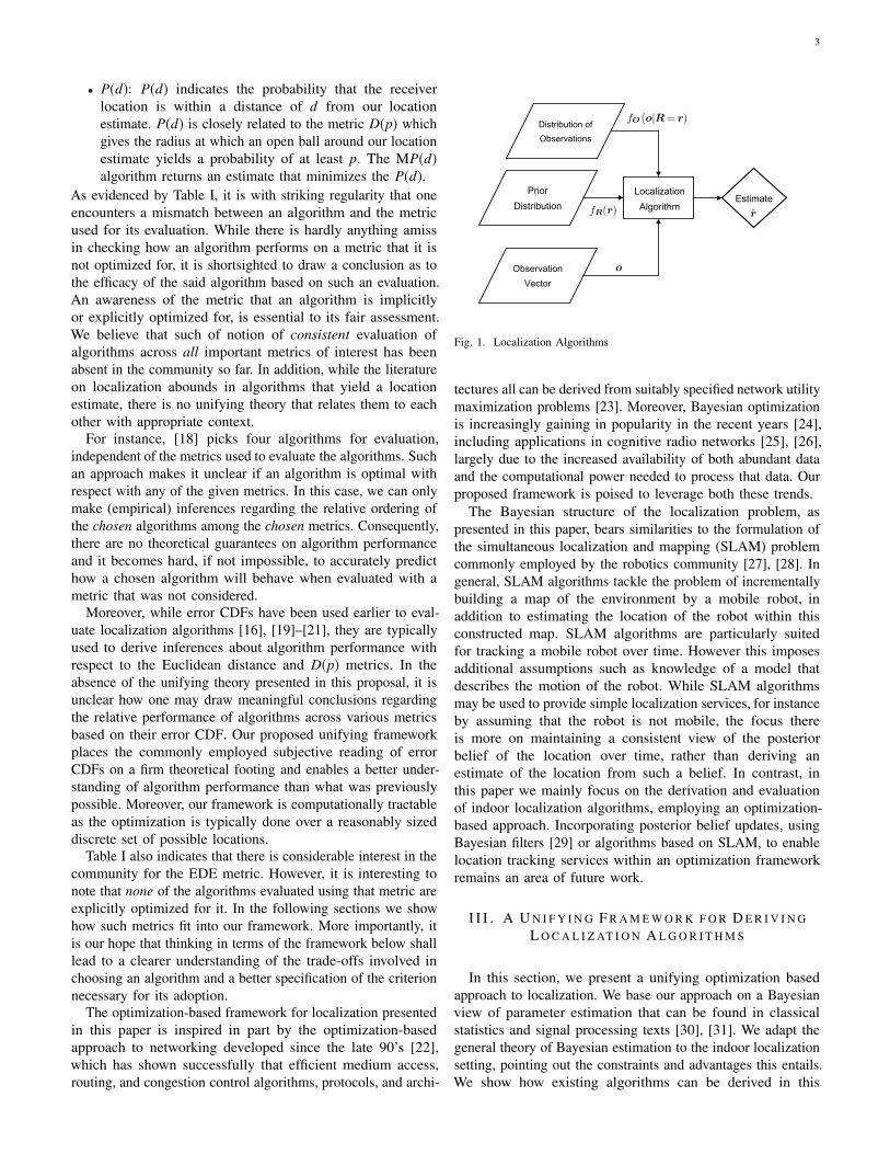
Localization Algorithm

Distribution of Observations

Prior Distribution

Observation Vector

Estimate

Fig. 1. Localization Algorithms

tectures all can be derived from suitably specified network utilitymaximization problems [23]. Moreover, Bayesian optimizationis increasingly gaining in popularity in the recent years [24],including applications in cognitive radio networks [25], [26],largely due to the increased availability of both abundant dataand the computational power needed to process that data. Ourproposed framework is poised to leverage both these trends.

The Bayesian structure of the localization problem, aspresented in this paper, bears similarities to the formulation ofthe simultaneous localization and mapping (SLAM) problemcommonly employed by the robotics community [27], [28]. Ingeneral, SLAM algorithms tackle the problem of incrementallybuilding a map of the environment by a mobile robot, inaddition to estimating the location of the robot within thisconstructed map. SLAM algorithms are particularly suitedfor tracking a mobile robot over time. However this imposesadditional assumptions such as knowledge of a model thatdescribes the motion of the robot. While SLAM algorithmsmay be used to provide simple localization services, for instanceby assuming that the robot is not mobile, the focus thereis more on maintaining a consistent view of the posteriorbelief of the location over time, rather than deriving anestimate of the location from such a belief. In contrast, inthis paper we mainly focus on the derivation and evaluationof indoor localization algorithms, employing an optimization-based approach. Incorporating posterior belief updates, usingBayesian filters [29] or algorithms based on SLAM, to enablelocation tracking services within an optimization frameworkremains an area of future work.

I I I . A U N I F Y I N G F R A M E W O R K F O R D E R I V I N GL O C A L I Z AT I O N A L G O R I T H M S

In this section, we present a unifying optimization basedapproach to localization. We base our approach on a Bayesianview of parameter estimation that can be found in classicalstatistics and signal processing texts [30], [31]. We adapt thegeneral theory of Bayesian estimation to the indoor localizationsetting, pointing out the constraints and advantages this entails.We show how existing algorithms can be derived in this

4

TABLE IIR E C O V E R I N G E X I S T I N G A L G O R I T H M S I N O U R F R A M E W O R K

Algorithm Cost function Optimization

MMSE C(r, r̃, o) = ( ‖r̃ − r ‖2)2 rMMSE = arg minr̃ E

[( ‖r̃ − r ‖2)

2]

MEDE C(r, r̃, o) = ‖r̃ − r ‖2 rMEDE = arg minr̃ E [ ‖r̃ − r ‖2]

MP(d) C(r, r̃, o) = −P ( ‖r̃ − r ‖2 ≤ d) rMP(d) = arg maxr̃ E [P (‖r̃ − r ‖2 ≤ d)]

MLE C(r, r̃, o) = −P ( ‖r̃ − r ‖2 ≤ ε ) rMLE = limε→0 arg maxr̃ E [P ( ‖r̃ − r ‖2 ≤ ε )]

framework and point out how alternate algorithms may bederived.

Let S ⊆ R2 be the two-dimensional space of interest inwhich localization is to be performed1. We assume that S isclosed and bounded. Let the location of the receiver (the nodewhose location is to be estimated) be denoted as r = [xr, yr ].Using a Bayesian viewpoint [30], [31], we assume that thislocation is a random variable with some prior distributionfR(r). This prior distribution is used to represent knowledgeabout the possible position, obtained, for instance from previouslocation estimates or knowledge of the corresponding user’smobility characteristics in the space; in the absence of any priorknowledge, it could be set to be uniform over S. Let o ∈ RN

represent the location dependent observation data that wascollected. As an example, o could represent the received signalstrength values from transmitters whose locations are known.Mathematically, we only require that the observation vector isdrawn from a known distribution that depends on the receiverlocation r: fO (o|R = r). In case of RSS measurements,this distribution characterizes the stochastic radio propagationcharacteristics of the environment and the location of thetransmitters. Note that this distribution could be expressedin the form of a standard fading model whose parametersare fitted with observed data, such as the well-known simplepath loss model with log-normal fading [32]. The distributionfO (o|R = r) is general enough to incorporate more data-drivenapproaches such as the well-known fingerprinting procedure.In fingerprinting, there is a training phase in which statisticalmeasurements are obtained at the receiver at various knownlocations and used to estimate the distribution of received signalstrengths at each location.2 Fundamentally, the data-drivenapproach constructs fO (o|R = r) empirically, while model-dependent approaches take the distribution over observationsdirectly from the model.

Using the conditional distribution of the observed vector andthe prior over R, we obtain the conditional distribution overthe receiver locations using Bayes’ rule:

fR (r |O = o) =fO(o|R = r) fR(r)∫

r∈SfO (o|R = r) fR(r) dr

. (1)

1It is trivial to extend the framework to 3-D localization, for simplicity, wefocus on the more commonly considered case of 2-D localization here.

2We note that in many implementations of fingerprinting, only the meanreceived signal strength from each transmitter is used, which of course is aspecial case, equivalent to assuming a deterministic signal strength measurementwith a unit step function cumulative distribution function.

Algorithms for localization are essentially methods that derivea location estimate from the above posterior distribution. Infact, any localization algorithm A is a mapping from• the observation vector o• the prior distribution over the location, fR(r)• the conditional distribution over o, fO (o|R = r)

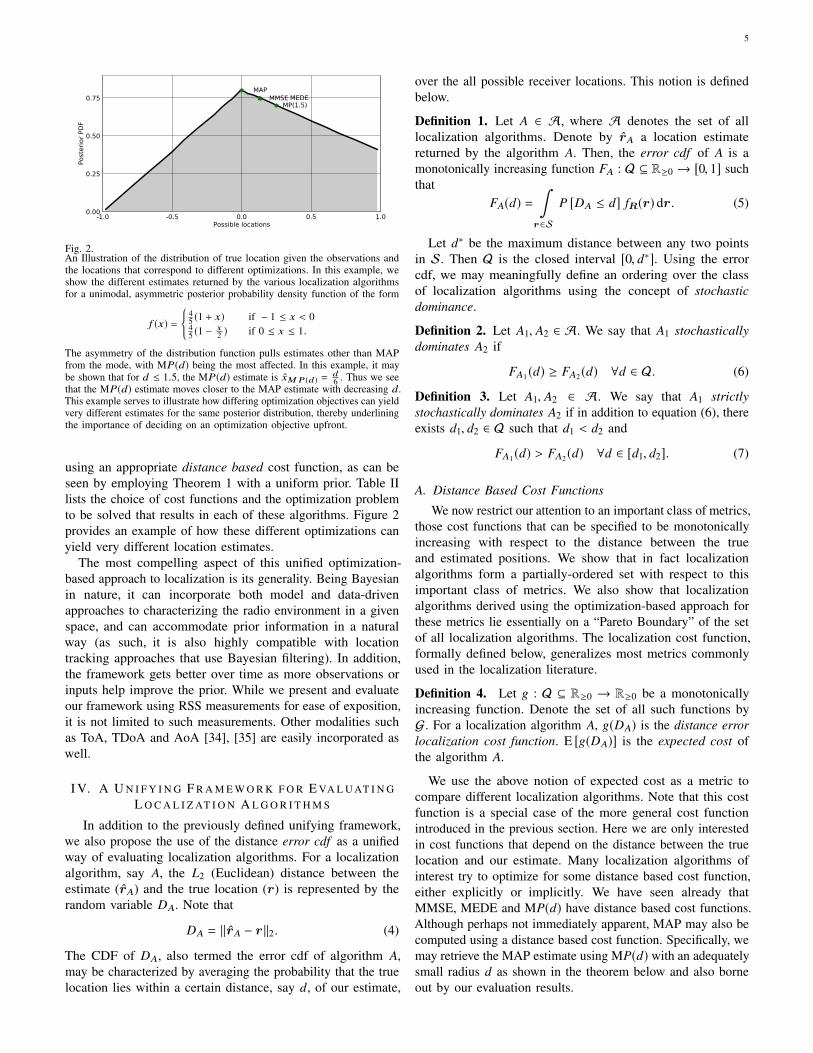
to a location estimate r̂, as illustrated in Figure 1. A visualiza-tion3 of the posterior distribution for the popular simple pathloss model with log-normal fading is given in Figure 3.

A. Optimization based approach to Localization

The starting point for estimating the receiver location is acost function that must be defined a priori. In the most generalterms, the cost function is modeled as C(r, r̃, o), i.e., a functionof the true location r, a given proposed location estimate r̃, andthe observation vector o. We define the expected cost functiongiven an observation vector as follows:

E[C(r, r̃, o)] =∫

r∈S

C(r, r̃, o) fR (r |O = o) dr. (2)

Given any cost function C, the optimal location estimationalgorithm can be obtained in a unified manner by solving thefollowing optimization for any given observation vector toobtain the optimal estimate r̂:

r̂ = arg minr̃

E[C(r, r̃, o)]. (3)

Note that this optimization may be performed to obtainan arbitrarily near-optimal solution by numerically computingE[C(r, r̃, o)] over the discretization of a two or three dimen-sional search space. Given recent gains in computing power, theoptimization is feasible for typical indoor localization problems.Moreover, the optimization naturally lends itself to parallelexecution since the computation of the expected cost at allcandidate locations are independent of each other. Assuminguniform coverage, the solution will improve upon increasingthe number of points in our search space. In practice, for RSSlocalization, these points could be spaced apart on the orderof 10’s of centimeters.

Existing algorithms such as MLE, MMSE, MEDE and MP(d)can be recovered in this framework using suitable choices of thecost function C. For instance, it is straightforward to verify thatminimizing the expected distance error yields MEDE. Perhapsmore interestingly, the MLE estimate can also be recovered

3The code used to generate the figures in this paper is available online [33].

5

-1.0 -0.5 0.0 0.5 1.0Possible locations

0.00

0.25

0.50

0.75

Post

erio

r PDF

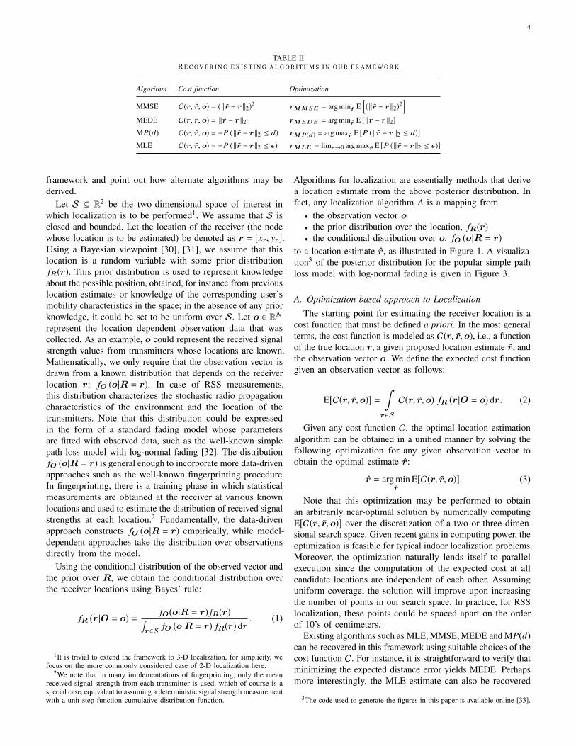
MMSEMAP

MEDEMP(1.5)

Fig. 2.An Illustration of the distribution of true location given the observations andthe locations that correspond to different optimizations. In this example, weshow the different estimates returned by the various localization algorithmsfor a unimodal, asymmetric posterior probability density function of the form

f (x) =

{45 (1 + x) if − 1 ≤ x < 045 (1 −

x2 ) if 0 ≤ x ≤ 1.

The asymmetry of the distribution function pulls estimates other than MAPfrom the mode, with MP(d) being the most affected. In this example, it maybe shown that for d ≤ 1.5, the MP(d) estimate is x̂MP(d) =

d6 . Thus we see

that the MP(d) estimate moves closer to the MAP estimate with decreasing d.This example serves to illustrate how differing optimization objectives can yieldvery different estimates for the same posterior distribution, thereby underliningthe importance of deciding on an optimization objective upfront.

using an appropriate distance based cost function, as can beseen by employing Theorem 1 with a uniform prior. Table IIlists the choice of cost functions and the optimization problemto be solved that results in each of these algorithms. Figure 2provides an example of how these different optimizations canyield very different location estimates.

The most compelling aspect of this unified optimization-based approach to localization is its generality. Being Bayesianin nature, it can incorporate both model and data-drivenapproaches to characterizing the radio environment in a givenspace, and can accommodate prior information in a naturalway (as such, it is also highly compatible with locationtracking approaches that use Bayesian filtering). In addition,the framework gets better over time as more observations orinputs help improve the prior. While we present and evaluateour framework using RSS measurements for ease of exposition,it is not limited to such measurements. Other modalities suchas ToA, TDoA and AoA [34], [35] are easily incorporated aswell.

I V. A U N I F Y I N G F R A M E W O R K F O R E VA L U AT I N GL O C A L I Z AT I O N A L G O R I T H M S

In addition to the previously defined unifying framework,we also propose the use of the distance error cdf as a unifiedway of evaluating localization algorithms. For a localizationalgorithm, say A, the L2 (Euclidean) distance between theestimate (r̂A) and the true location (r) is represented by therandom variable DA. Note that

DA = ‖r̂A − r‖2. (4)

The CDF of DA, also termed the error cdf of algorithm A,may be characterized by averaging the probability that the truelocation lies within a certain distance, say d, of our estimate,

over the all possible receiver locations. This notion is definedbelow.

Definition 1. Let A ∈ A, where A denotes the set of alllocalization algorithms. Denote by r̂A a location estimatereturned by the algorithm A. Then, the error cdf of A is amonotonically increasing function FA : Q ⊆ R≥0 → [0, 1] suchthat

FA(d) =∫

r∈S

P [DA ≤ d] fR(r) dr. (5)

Let d∗ be the maximum distance between any two pointsin S. Then Q is the closed interval [0, d∗]. Using the errorcdf, we may meaningfully define an ordering over the classof localization algorithms using the concept of stochasticdominance.

Definition 2. Let A1, A2 ∈ A. We say that A1 stochasticallydominates A2 if

FA1 (d) ≥ FA2 (d) ∀d ∈ Q. (6)

Definition 3. Let A1, A2 ∈ A. We say that A1 strictlystochastically dominates A2 if in addition to equation (6), thereexists d1, d2 ∈ Q such that d1 < d2 and

FA1 (d) > FA2 (d) ∀d ∈ [d1, d2]. (7)

A. Distance Based Cost Functions

We now restrict our attention to an important class of metrics,those cost functions that can be specified to be monotonicallyincreasing with respect to the distance between the trueand estimated positions. We show that in fact localizationalgorithms form a partially-ordered set with respect to thisimportant class of metrics. We also show that localizationalgorithms derived using the optimization-based approach forthese metrics lie essentially on a “Pareto Boundary” of the setof all localization algorithms. The localization cost function,formally defined below, generalizes most metrics commonlyused in the localization literature.

Definition 4. Let g : Q ⊆ R≥0 → R≥0 be a monotonicallyincreasing function. Denote the set of all such functions byG. For a localization algorithm A, g(DA) is the distance errorlocalization cost function. E [g(DA)] is the expected cost ofthe algorithm A.

We use the above notion of expected cost as a metric tocompare different localization algorithms. Note that this costfunction is a special case of the more general cost functionintroduced in the previous section. Here we are only interestedin cost functions that depend on the distance between the truelocation and our estimate. Many localization algorithms ofinterest try to optimize for some distance based cost function,either explicitly or implicitly. We have seen already thatMMSE, MEDE and MP(d) have distance based cost functions.Although perhaps not immediately apparent, MAP may also becomputed using a distance based cost function. Specifically, wemay retrieve the MAP estimate using MP(d) with an adequatelysmall radius d as shown in the theorem below and also borneout by our evaluation results.

6

X

5

10

15

Y5

10

15

0.0002

0.0004

0.0006

(a)

X

5

10

15

Y5

10

15

0.00025

0.00050

0.00075

(b)

X

5

10

15

Y5

10

15

0.00025

0.00050

0.00075

(c)

X

5

10

15

Y5

10

15

0.0002

0.0004

0.0006

(d)

Fig. 3. Illustration of the posterior distribution of R using observations taken from a log-normal distribution. For this illustration, four transmitters were placedin a 16 m × 16 m area. A log-normal path loss model was used to to determine the signal strengths. Each subplot above shows the posterior distribution of Rconstructed by the receiver upon receiving a different vector of observations.

Theorem 1. If the posterior distribution fR |O is continuousand the MAP estimate lies in the interior of S, then for anyδ > 0 there exists ε > 0 such that,

|P1(d) − P2(d)| ≤ δ ∀ 0 < d < ε, (8)

where P1(d) and P2(d) give the probability of the receiverlocation being within distance d of the MAP and the MP(d)estimate respectively.

Proof. See Appendix. �

B. Comparing Algorithms using Stochastic Dominance

In this section, we explore how we may meaningfullycompare algorithms using our optimization based framework. Ifwe are interested in a particular cost function, then comparingtwo algorithms is straightforward. Compute their expectedcost and the algorithm with the lower cost is better. However,with stochastic dominance we can deduce something morepowerful. For any two localization algorithms A1 and A2, ifA1 stochastically dominates A2, then the expected cost of A1does not exceed that of A2 for any distance based cost function.More formally,

Theorem 2. For any two localization algorithms A1, A2 ∈ A,if A1 stochastically dominates A2, then

E[g(DA1 )

]≤ E

[g(DA2 )

] ∀g ∈ G. (9)

If A1 strictly stochastically dominates A2, then

E[g(DA1 )

]< E

[g(DA2 )

] ∀g ∈ G. (10)

Proof. See Appendix. �

Theorem 2 is the first step towards ranking algorithms basedon stochastic dominance. It also gives us a first glimpse ofwhat an optimal algorithm might look like. From Theorem 2,an algorithm A∗ that stochastically dominates every otheralgorithm is clearly optimal for the entire set of distance basedcost functions. However, it is not obvious that such an algorithmneed even exist. On the other hand, we can compute algorithmsthat are optimal with respect to a particular cost function. Asgiven in the following theorem, such optimality implies that thealgorithm isn’t strictly dominated by any other algorithm. Inother words, if algorithm A is optimal with respect to a distancebased cost function g, then A is not strictly stochasticallydominated by any other algorithm B.

7

Theorem 3. For a localization algorithm A ∈ A, if thereexists a distance based cost function g ∈ G such that for anyother localization algorithm B ∈ A

E [g (DA)] ≤ E [g (DB)] , (11)

then for all algorithms B ∈ A, there exists a distance d ∈ Qsuch that

FA(d) ≥ FB(d). (12)

Proof. See Appendix. �

Theorems 2 & 3 establish the utility of ranking algorithmsbased on stochastic dominance. However, if we are given twoalgorithms, it is not necessary that one should dominate the other.As Theorem 4 shows, if they do not conform to a stochasticdominance ordering, the algorithms are incomparable.

Theorem 4. For any two localization algorithms A1 and A2,if A2 does not stochastically dominate A1 and vice versa, thenthere exits distance based cost functions g1, g2 ∈ G such that

E[g1(DA1 )

]< E

[g1(DA2 )

], (13)

andE

[g2(DA2 )

]< E

[g2(DA1 )

]. (14)

Proof. See Appendix. �

Theorem 4 establishes the existence of a “Pareto Boundary”of the set of all localization algorithms. Choosing an algorithmfrom within this set depends on additional considerations suchas its performance on specific cost functions of interest.

C. Comparison based on Upper Bound of Error CDFs

In the previous section, we focused on using stochasticdominance to rank and compare algorithms without payingmuch attention to what an ideal algorithm might look like. Inthis section, we explore this topic more detail. To begin, weask if there exists an algorithm that dominates every otheralgorithm? From Theorem 2 we know that such an algorithm,if it exists, will be the best possible algorithm for the class ofdistance based cost functions. Moreover the error CDF of suchan algorithm will be an upper bound on the error CDFs of allalgorithms A ∈ A.

Definition 5. We denote the upper envelope of error CDFsfor all possible algorithms A ∈ A by F∗.

We now turn our attention to formally defining the errorbound F∗. Our definition also provides us with a way tocompute F∗. Let DA represent the distance error for algorithmA. Consider the following class of MP(d) cost functions. Foreach d ∈ Q, let

gd (D) =

{0 if D ≤ d1 if D > d.

(15)

Then, the value of F∗ at any distance d ∈ Q may be computedusing the MP(d) cost function at that distance. More formally,

Definition 6. The upper envelope of error CDFs for all possiblealgorithms A ∈ A, F∗ is defined as

F∗(d) = supA∈A{1 − E [gd(DA)]} , ∀d ∈ Q. (16)

The upper envelope of error CDFs, F∗, satisfies the followingproperties:

1) F∗ stochastically dominates every algorithm A ∈ A,2) F∗ is monotonically increasing in [0, d∗],3) F∗ is Riemann integrable over [0, d∗].

The monotonicity of F∗ is direct consequence of the mono-tonicity of CDFs. Moreover, since F∗ is monotonic, it is alsoRiemann integrable [36, p. 126]. In general, F∗ may notbe attainable by any other algorithm. However, as we showbelow, it is achievable under certain circumstances, which lendscredence to its claim as a useful upper bound that may be usedas a basis of comparison of localization algorithms.

Given the ideal performance characteristics of F∗, it isworthwhile to investigate if it is ever attained by an algorithm.A trivial case is when the MP(d) algorithm yields the sameestimate for all distances of interest in the domain. In thisparticular case, MAP and MP(d) are optimal since the errorCDF of the MAP or MP(d) estimate traces F∗. As anillustration consider a continuous symmetric unimodal posteriordistribution over a circular space with the mode located onthe center of the circle. Clearly, the MAP estimate is given bythe center. Moreover, the MP(d) estimate is the same at alldistances, namely the center of the circle. Thus we immediatelyhave that both the MAP and MP(d) estimates have attainedF∗. An extensive discussion on the attainability of F∗ can befound in Appendix F.

Thus we see that there exist conditions under which F∗ isattained by an algorithm. Consequently, it is worthwhile tosearch for algorithms that are close to this bound or even attainit under more general settings. This leads us directly to thesecond method of comparing algorithms. We identify how closethe error CDFs of our algorithms get to the upper bound F∗.

Consider algorithms A, B ∈ A. Intuitively, if the error CDFof A is closer to F∗ than that of B, then it seems reasonableto expect A to perform better. To make this idea precise,we need to define our measure of closeness to F∗. In thefollowing paragraph, we propose one such measure of howclose the error CDF of an algorithm A is to F∗. Our proposalsatisfies a nice property. Namely, searching for an algorithmthat is optimal over this measure is equivalent to searching foran algorithm that minimizes a particular distance based costfunction. Consequently, to specify the algorithm we only needto identify this cost function.

Definition 7. The area between the error CDF of algorithm Aand the upper envelope of error CDFs is given by

ΘA =

d∗∫0

(F∗(x) − FA(x)) dx. (17)

The intuition behind our measure is can be summarizedeasily. We seek to find an algorithm A that minimizes the “areaenclosed” by F∗ and the error CDF of A. Note that ΘA ≥ 0

8

-100 -80 -60 -40O

0.0

0.1

0.2

0.3

0.4

f O(o

|R=

r)

(a)

-100 -80 -60 -40O

0.00

0.05

0.10

0.15

0.20

0.25

f O(o

|R=

r)

(b)

-100 -80 -60 -40O

0.0

0.1

0.2

0.3

f O(o

|R=

r)

(c)

-100 -80 -60 -40O

0.000

0.025

0.050

0.075

0.100

0.125

f O(o

|R=

r)

(d)

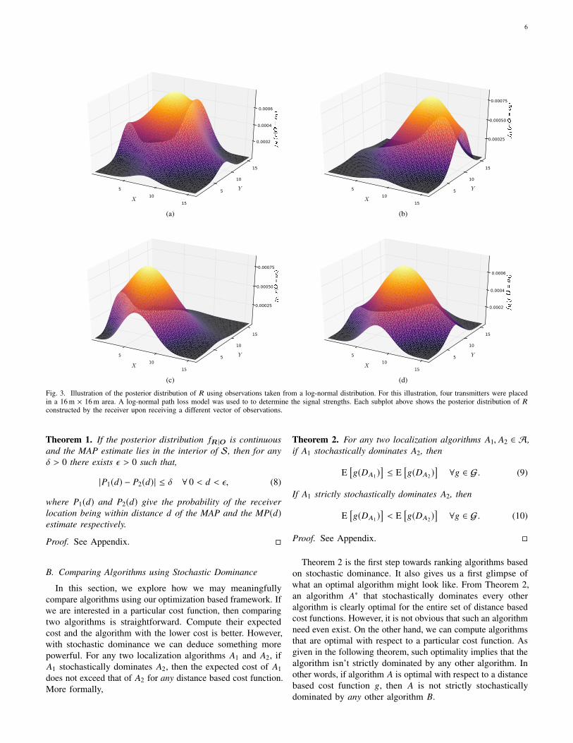
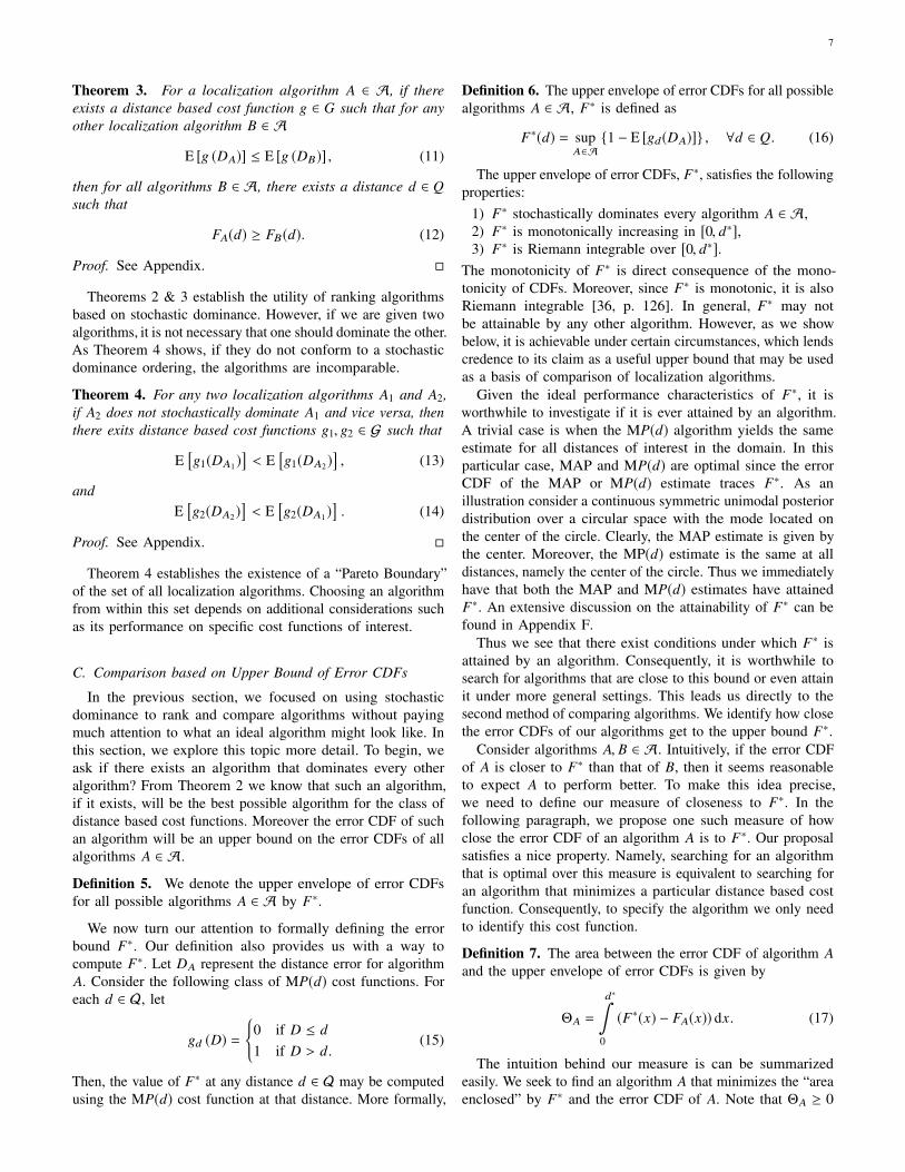
Fig. 4. Illustration of the empirically estimated distribution of O using signal strength measurements taken at different locations. Each subplot refers to thedistribution of signal strength from a unique access point. The left subplots refer to measurements taken at night, while the right subplots refer to measurementstaken during daytime. Our framework makes better use of the higher variance data.

for all A ∈ A. In general, it is not clear if every measure ofcloseness between F∗ and FA will yield a cost function forus to minimize. However, if we do find such a cost function,then we have the advantage of not needing to explicit knowF∗ in the execution of our algorithm. This is the case for ΘA

as proved in the theorem below.

Theorem 5. The algorithm that minimizes the area betweenits error CDF and the upper envelope of error CDFs for allpossible algorithms is the MEDE algorithm.

Proof. See Appendix. �

As consequence of Theorem 5, we note that if F∗ is attainableby any localization algorithm, then it is attained by MEDE.This in turn yields a simple test for ruling out the existenceof an algorithm that attains F∗. On plotting the error CDFplots of different algorithms, if we find an algorithm that isnot dominated by MEDE, then we may conclude that F∗ isunattainable. Thus it is relatively easy to identify cases wherethere is a gap between F∗ and MEDE. However, the issue ofconfirming that MEDE has attained F∗ is more difficult as itinvolves a search over the set of all algorithms.

In summary, the utility of F∗ lies in its ability to pin pointthe strengths and weaknesses of a proposed algorithm. As we

have seen, some algorithms such as MP(d) is designed to dowell at specific distances while others such as MEDE aims forsatisfactory performance at all distances. Other algorithms liesomewhere in between. Consequently, choosing one algorithmover the other depends on the needs of the application utilizingthe localization algorithm. Therein lies the strength of ourproposed framework. It allows us to effectively reason aboutthe applicability of an algorithm for the use case at hand.

D. Comparison with the Cramér–Rao Bound

The Cramér–Rao Bound (CRB) is often used as an aid inevaluating localization algorithms [14], [17], [37], [38]. How-ever, the CRB is not necessarily a good choice as an absolutemeasure of performance for every localization algorithm.

Let DA denote the distance error corresponding to a algo-rithm A. Define dA = E [DA]. Since the ideal distance error is0, dA is the bias of algorithm A. The expected mean squarederror of algorithm A may be then expressed as

E[D2

A

]= E

[(DA − dA)

2] + d2A (18)

= Var[DA] + (Bias[DA])2. (19)

In our setting, the CRB is a lower bound on Var[DA]. Thusan algorithm that attains the CRB is optimal only if (i) our

9

objective is to minimize the mean squared error, and (ii) theclass of algorithms under consideration is unbiased. In ourframework, the MMSE algorithm given in Table II shares thesame objective as that of an algorithm evaluated against theCRB. However, the MMSE algorithm considers both varianceand bias simultaneously, allowing for estimates that have asmall, non-zero bias combined with a small variance.

V. E VA L U AT I O N

We evaluate the proposed framework using simulations,traces and real world experiments. In Section V-A, we providean illustration of how fingerprinting methods fit in to theframework presented in Section III, using real-world datacollected from an indoor office environment. We show thatwhile many implementations of fingerprinting use only themean signal strength from each transmitter, we are able to betterutilize the collected data by building an empirical distributionof the received observations.

We also evaluate the performance of the MLE, MP(d),MMSE and MEDE using simulations as well as using traces [7].In both cases the signal propagation was modelled using asimplified path loss model with log-normal shadowing [32].We assume that the prior distribution ( fR) is uniform over S.

A. Fingerprinting Methods

Model-based methods assume that the distribution of ob-servations given a receiver location is known. In contrast,fingerprinting methods avoid the need to model the distributionof observations by noting that one only needs to identify thechange in distribution of observations from one location toanother. Most implementations simplify matters even furtherby assuming that mean of the observations is distinct acrossdifferent locations in our space of interest. The estimated meanis thus said to ‘fingerprint’ the location.

This approach works well only in cases when the distributionof signal strengths is mostly concentrated around the mean. Inthis case, the approach of using only the mean signal strengthamounts to approximating the signal strength distributionwith a normal distribution centered at the estimated meansignal strength and variance approaching zero. However, ifthe distribution has significant variance this approach is likelyto fail. Indeed, in the regime of significantly varying signalstrengths, keeping only the mean amounts to throwing awaymuch of the information that one has already taken pains tocollect.

As already indicated in Section III, we make better use ofthe collected data by empirically constructing the distributionof observations fO (o|R = r). This formulation allows us tothe use the same algorithms as in the model-based approach, asthe only difference here is in the construction of fO (o|R = r).This is in contrast to many existing implementations whereone resorts to heuristics such as clustering. Indeed, under mildassumptions it is well known that the empirical distributionconverges with probability one to true distribution [39] whichgives our approach the nice property that it can always dobetter given more data.

As a proof-of-concept, we compare the performance of ourapproach with that of traditional fingerprinting methods in twodifferent settings. The data was collected from a 4 m×2 m spaceinside an office environment. The space was divided into eight1 m × 1 m squares and signal strength samples were collectedfrom the center of each square. Two hundred and fifty signalstrength readings were collected for the ten strongest accesspoints detected using the WiFi card on a laptop running Linux.The beacon interval for each access point was approximately100 ms. The signal strength measurements were taken 400 msapart. Two sets of data were collected, one at night time and theother during the day. The measurements taken at night show thatthe observed signal strengths are highly concentrated aroundthe mean, as can be seen from the left subplots of Figure 4.The measurements taken during daytime show slightly morevariability as can be seen in the right subplots of Figure 4.

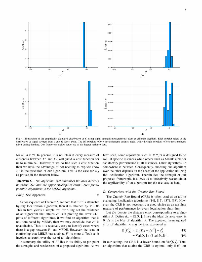
Ten percent of the collected data is randomly chosen forevaluating algorithm performance. The remaining data is usedto construct the empirical distribution f̂O (o|R = r) from whichthe MMSE, MAP and MEDE estimates are derived. It is alsoused to compute the mean signal strength vector or fingerprintfor each location. For the algorithm denoted as ‘FING’ inFigure 5, the fingerprint closest to the test observation vector(in terms of Euclidean distance) is used to predict the location.

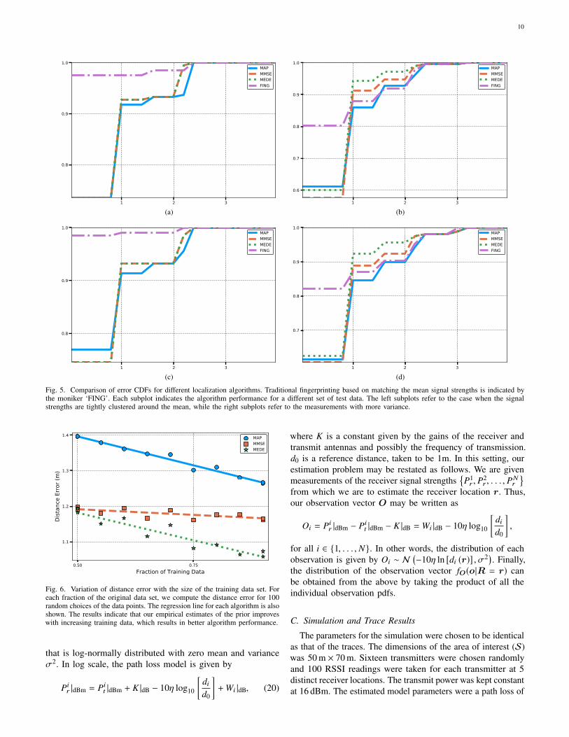
From the performance results given in Figure 5, we see that,as expected, the traditional fingerprinting approach works verywell when the variability in the signal strength data is low.On the other hand, even with slight variability in the data, theestimates derived using our Bayesian framework outperformstraditional fingerprinting.

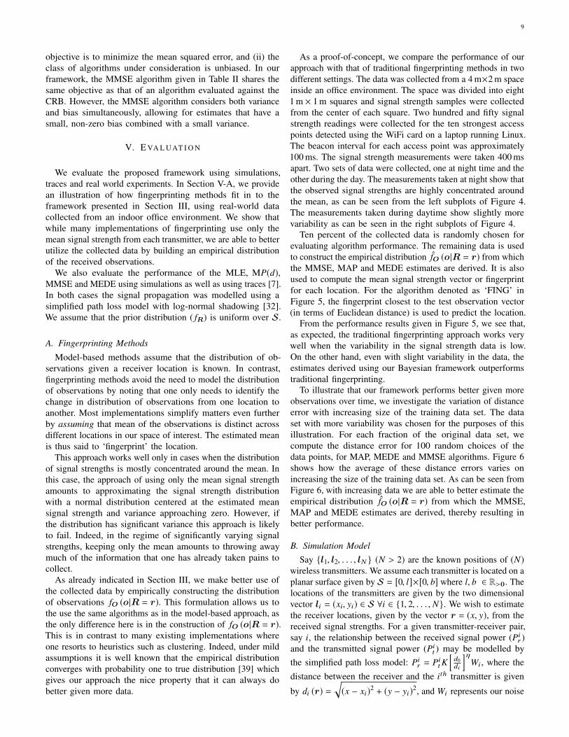
To illustrate that our framework performs better given moreobservations over time, we investigate the variation of distanceerror with increasing size of the training data set. The dataset with more variability was chosen for the purposes of thisillustration. For each fraction of the original data set, wecompute the distance error for 100 random choices of thedata points, for MAP, MEDE and MMSE algorithms. Figure 6shows how the average of these distance errors varies onincreasing the size of the training data set. As can be seen fromFigure 6, with increasing data we are able to better estimate theempirical distribution f̂O (o|R = r) from which the MMSE,MAP and MEDE estimates are derived, thereby resulting inbetter performance.

B. Simulation ModelSay {l1, l2, . . . , lN } (N > 2) are the known positions of (N)

wireless transmitters. We assume each transmitter is located on aplanar surface given by S = [0, l]×[0, b] where l, b ∈ R>0. Thelocations of the transmitters are given by the two dimensionalvector li = (xi, yi) ∈ S ∀i ∈ {1, 2, . . . , N}. We wish to estimatethe receiver locations, given by the vector r = (x, y), from thereceived signal strengths. For a given transmitter-receiver pair,say i, the relationship between the received signal power (Pi

r )and the transmitted signal power (Pi

t ) may be modelled bythe simplified path loss model: Pi

r = PitK

[d0di

]ηWi , where the

distance between the receiver and the ith transmitter is given

by di (r) =√(x − xi)2 + (y − yi)

2, and Wi represents our noise

10

1 2 3

0.8

0.9

1.0MAPMMSEMEDEFING

(a)1 2 3

0.6

0.7

0.8

0.9

1.0MAPMMSEMEDEFING

(b)

1 2 3

0.8

0.9

1.0MAPMMSEMEDEFING

(c)1 2 3

0.7

0.8

0.9

1.0MAPMMSEMEDEFING

(d)

Fig. 5. Comparison of error CDFs for different localization algorithms. Traditional fingerprinting based on matching the mean signal strengths is indicated bythe moniker ‘FING’. Each subplot indicates the algorithm performance for a different set of test data. The left subplots refer to the case when the signalstrengths are tightly clustered around the mean, while the right subplots refer to the measurements with more variance.

0.50 0.75Fraction of Training Data

1.1

1.2

1.3

1.4

Dist

ance

Erro

r (m

)

MAPMMSEMEDE

Fig. 6. Variation of distance error with the size of the training data set. Foreach fraction of the original data set, we compute the distance error for 100random choices of the data points. The regression line for each algorithm is alsoshown. The results indicate that our empirical estimates of the prior improveswith increasing training data, which results in better algorithm performance.

that is log-normally distributed with zero mean and varianceσ2. In log scale, the path loss model is given by

Pir |dBm = Pi

t |dBm + K |dB − 10η log10

[did0

]+Wi |dB, (20)

where K is a constant given by the gains of the receiver andtransmit antennas and possibly the frequency of transmission.d0 is a reference distance, taken to be 1m. In this setting, ourestimation problem may be restated as follows. We are givenmeasurements of the receiver signal strengths

{P1r , P

2r , . . . , P

Nr

}from which we are to estimate the receiver location r. Thus,our observation vector O may be written as

Oi = Pir |dBm − Pi

t |dBm − K |dB = Wi |dB − 10η log10

[did0

],

for all i ∈ {1, . . . , N}. In other words, the distribution of eachobservation is given by Oi ∼ N

(−10η ln [di (r)] , σ2) . Finally,

the distribution of the observation vector fO(o|R = r) canbe obtained from the above by taking the product of all theindividual observation pdfs.

C. Simulation and Trace Results

The parameters for the simulation were chosen to be identicalas that of the traces. The dimensions of the area of interest (S)was 50 m × 70 m. Sixteen transmitters were chosen randomlyand 100 RSSI readings were taken for each transmitter at 5distinct receiver locations. The transmit power was kept constantat 16 dBm. The estimated model parameters were a path loss of

11

TABLE IIIN O R M A L I Z E D P E R F O R M A N C E R E S U LT S

Simulations

Likelihood P(ε ) P(d) MSE EDE

MLE 1.0000 0.9222 0.8994 1.4359 1.1240

MP(ε ) 0.9808 1.0000 0.9165 1.3172 1.0997

MP(d) 0.6963 0.7573 1.0000 1.2860 1.0857

MMSE 0.6806 0.6980 0.8737 1.0000 1.0643

MEDE 0.7247 0.7455 0.9080 1.1272 1.0000

Traces

Likelihood P(ε ) P(d) MSE EDE

MLE 1.0000 0.9989 0.9865 1.1583 1.1808

MP(ε ) 0.9976 1.0000 0.9881 1.1522 1.1785

MP(d) 0.8213 0.8596 1.0000 1.2605 1.3760

MMSE 0.9013 0.9171 0.9797 1.0000 1.1101

MEDE 0.8529 0.8685 0.9517 1.1569 1.0000

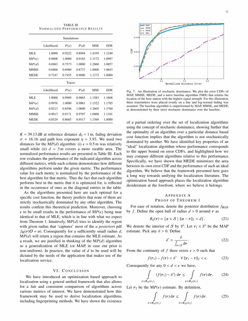
K = 39.13 dB at reference distance d0 = 1 m, fading deviationσ = 16.16 and path loss exponent η = 3.93. We used twodistances for the MP(d) algorithm: (i) ε = 0.5 m was relativelysmall while (ii) d = 3 m covers a more sizable area. Thenormalized performance results are presented in Table III. Eachrow evaluates the performance of the indicated algorithm acrossdifferent metrics, while each column demonstrates how differentalgorithms perform under the given metric. The performancevalue for each metric is normalized by the performance of thebest algorithm for that metric. Thus the fact that each algorithmperforms best in the metric that it is optimized for, is reflectedin the occurrence of ones as the diagonal entries in the table.

As the algorithms presented here are each optimal for aspecific cost function, the theory predicts that none of them arestrictly stochastically dominated by any other algorithm. Theresults confirm this theoretical prediction. Moreover, choosingε to be small results in the performance of MP(ε) being nearidentical to that of MLE, which is in line with what we expectfrom Theorem 1. Intuitively, MP(d) tries to identify the regionwith given radius that ‘captures’ most of the a posteriori pdffR(r |O = o). Consequently for a sufficiently small radius d,MP(d) will return a region that contains the MLE estimate. Asa result, we are justified in thinking of the MP(d) algorithmas a generalization of MLE (or MAP, in case our prior isnon-uniform). In practice, the value of d to be used will bedictated by the needs of the application that makes use of thelocalization service.

V I . C O N C L U S I O N

We have introduced an optimization based approach tolocalization using a general unified framework that also allowsfor a fair and consistent comparison of algorithms acrossvarious metrics of interest. We have demonstrated how thisframework may be used to derive localization algorithms,including fingerprinting methods. We have shown the existence

0.2 0.4 0.6Normalized Distance Error

0.25

0.50

0.75

CDF

MAPMMSEMEDENBS

Fig. 7. An illustration of stochastic dominance. We plot the error CDFs ofMAP, MMSE, MEDE, and a naïve baseline algorithm (NBS) that returns thelocation of the base station with the highest signal strength. For this illustration,three transmitters were placed evenly on a line and log-normal fading wasassumed. The baseline algorithm is outperformed by MAP, MMSE, and MEDE,as demonstrated by their strict stochastic dominance over the baseline.

of a partial ordering over the set of localization algorithmsusing the concept of stochastic dominance, showing further thatthe optimality of an algorithm over a particular distance basedcost function implies that the algorithm is not stochasticallydominated by another. We have identified key properties of an“ideal” localization algorithm whose performance correspondsto the upper bound on error CDFs, and highlighted how wemay compare different algorithms relative to this performance.Specifically, we have shown that MEDE minimizes the areabetween its own error CDF and the performance of such an idealalgorithm. We believe that the framework presented here goesa long way towards unifying the localization literature. Theoptimization based approach places the localization algorithmdesideratum at the forefront, where we believe it belongs.

A P P E N D I X AP R O O F O F T H E O R E M 1

For ease of notation, denote the posterior distribution fR |Oby f . Define the open ball of radius d > 0 around r as

Bd(r) = {x ∈ S | ‖x − r‖2 < d} . (21)

We denote the interior of S by So. Let r1 ∈ So be the MAPestimate. Pick any δ > 0. Define

δ′ =δ∫

r∈Sdr. (22)

From the continuity of f there exists ε > 0 such that

f (r1) − f (r) < δ′ ∀ ‖r1 − r‖2 < ε. (23)

Consequently for any 0 < d < ε we have,∫r∈Bd (r1)

( f (r1) − δ′) dr ≤

∫r∈Bd (r1)

f (r) dr. (24)

Let r2 be the MP(ε) estimate. By definition,∫r∈Bd (r1)

f (r) dr ≤∫

r∈Bd (r2)

f (r) dr. (25)

12

Since r1 is the MAP estimate,∫r∈Bd (r2)

f (r) dr ≤∫

r∈Bd (r2)

f (r1) dr. (26)

Combining the above inequalities together, we conclude

( f (r1) − δ′)

∫r∈Bd (r1)

dr ≤ P1(d) ≤ P2(d) ≤ f (r1)

∫r∈Bd (r2)

dr.

(27)

Note that the difference between the upper and lower bounds inthe above inequality is at most δ. Consequently, the difference|P1(d) − P2(d)| is also bounded by δ,

|P1(d) − P2(d)| ≤ δ ∀ 0 < d < ε. (28)

�

A P P E N D I X BP R O O F O F T H E O R E M 2

Recall that the domain of the cost function is given byQ ⊆ R≥0. For any element p in the range of the cost function,the inverse image of p is given by

g−1(p) = {d ∈ Q | g(d) = p} . (29)

Let h(p) = inf(g−1(p)

). From the monotonicity of g(d), we

conclude that h(p) is monotonically increasing in p. Moreover,we have the following relation for any algorithm A ∈ A

P (g(DA) ≤ p) = P (DA ≤ h(p)) . (30)

This allows us to characterize the CDF of g(DA) asFA (h (g(dA))). Moreover, since cost functions are non-negative,g(DA) ≥ 0. Thus the expected value of g(DA) for any algorithmA may be expressed as

E [g(DA)] =

sup(Q)∫0

(1 − FA (h (g(dA)))) ddA. (31)

Consider any two algorithms A1 and A2 such that A1 stochas-tically dominates A2. From (6), we have

FA1 (h (g(d))) ≥ FA2 (h (g(d))) ∀d ∈ Q. (32)

From (31) and (32), we conclude

E[g(DA1 )

]≤ E

[g(DA2 )

], (33)

which proves (9). If A1 strictly dominates A2, then in additionto (32), A1 and A2 satisfies

FA1 (h (g(d))) > FA2 (h (g(d))) ∀d ∈ [d1, d2]. (34)

From (31), (32) and (34) we have

E[g(DA1 )

]< E

[g(DA2 )

]. (35)

�

A P P E N D I X CP R O O F O F T H E O R E M 3

Say A ∈ A is the optimal algorithm for the distance basedcost function g ∈ G. Further assume that for some algorithmB ∈ A,

FA(d) ≤ FB(d) ∀d ∈ Q, (36)

and that there exists some d ′ ∈ Q such that FA(d ′) < FB(d ′).If these conditions implied that A is strictly dominated by B,then by Theorem 2 we have

E [g(DA)] > E [g(DB)] . (37)

However, from the optimality of A with respect to g,

E [g(DA)] ≤ E [g(DB)] , (38)

which contradicts (37). To complete the proof of Theorem 3we need to show the strict dominance of B over A. Since theerror CDFs are right continuous, for any ε > 0 there exists aδ > 0 such that

FB(d) − FB(d ′) < ε ∀d ∈ [d ′, d ′ + δ], (39)

and

FA(d) − FA(d ′) < ε ∀d ∈ [d ′, d ′ + δ]. (40)

Choosing ε < FB (d′)−FA(d

′)

2 implies

FB(d) > FA(d) ∀d ∈ [d ′, d ′ + δ], (41)

which proves that B strictly dominates A. �

A P P E N D I X DP R O O F O F T H E O R E M 4

Since A2 does not stochastically dominate A1, there existssome d1 ∈ Q such that

FA1 (d1) > FA2 (d1) . (42)

Since A1 does not stochastically dominate A2, there exists somed2 ∈ Q such that

FA1 (d2) < FA2 (d2) . (43)

Define the cost functions g1 and g2 as

g1 (D) =

{0 if D ≤ d1

1 if D > d1,(44)

and

g2 (D) =

{0 if D ≤ d2

1 if D > d2.(45)

Thus,

E[g1(DA1 )

]= 1 − FA1 (d1) (46)

< 1 − FA2 (d1) = E[g1(DA2 )

], (47)

where the inequality follows from (42). Similarly,

E[g2(DA2 )

]= 1 − FA2 (d2) (48)

< 1 − FA1 (d2) = E[g2(DA1 )

], (49)

where the inequality in the second step follows from (43). �

13

A P P E N D I X EP R O O F O F T H E O R E M 5

As F∗ dominates every other algorithm, the area under theCDF curve of any other algorithm is no greater than thearea under F∗. Consequently, maximizing RA is equivalentto maximizing the area under the CDF curve of the algorithm.We use this fact to show that the expected distance errorof algorithm A, E [DA] is a linear function of RA. Thus analgorithm that minimizes RA minimizes E [DA] as well andvice versa. More formally, for all A ∈ A

RA =

d∗∫0

(F∗(x) − FA(x)) dx (50)

=

d∗∫0

(1 − FA(x)) dx +

d∗∫0

(F∗(x) − 1) dx (51)

= E [DA] + α, (52)

where the last equality follows from the fact that the randomvariable DA is non-negative and α is the constant given byα =

∫ d∗

0 (F∗(x) − 1) dx. �

A P P E N D I X FAT TA I N A B I L I T Y O F T H E O P T I M A L E R R O R C D F

As indicated in Section IV-C, if we have a symmetricunimodal distribution over a circular area with the mode locatedat the center, then the MAP estimate is optimal. On the otherhand, from an algorithmic perspective, MEDE has the niceproperty, following Theorem 3, that if there exists an algorithmthat attains F∗, then the MEDE algorithm will attain it aswell. However, it is not clear a priori if F∗ is attainable. Asufficient and necessary condition for the attainability F∗ maybe obtained in light of the following observations:• By design, the MP(d) estimate matches the performance

of F∗ for the specific distance d ∈ Q. However, there areno guarantees on the performance the estimate at otherdistances.

• The MP(d) algorithm need not return a unique locationestimate. This reflects the fact that there may be multiplelocations in S that maximizes the P(d) metric for thegiven posterior distribution.

Consequently, consider a modified version of the MP(d)algorithm that enumerates all possible MP(d) estimates for thegiven distance d. If F∗ is attainable by some algorithm A, thenthe estimate returned by A, say r̂A, must exist in the list returnedby the MP(d) algorithm. Note that this condition holds for anydistance d ∈ Q used for the MP(d) algorithm. Consequently,if the intersection of the estimate list returned by MP(d) forall d ∈ Q is non-empty, then we conclude that F∗ is attainedby each estimate in the intersection. If the intersection is a nullset, then we conclude that F∗ is unattainable, thereby givingus the necessary and sufficient condition for the existence ofF∗.

While the above test calls for the repeated execution of theMP(d) algorithm over a potentially large search space, we mayexploit the fact that each execution is independent of each

other, thereby gaining considerable speed improvements byutilizing parallel processing. In some cases, it may be possibleto carry out this test analytically. The condition enumeratedin Section IV-C is a case in point. The task of identifying thecases when we can obtain the algorithm that attains F∗ is atopic of future research. A slight generalization of the examplegiven in Section IV-C leads to the following conjecture.

Conjecture 1. If the posterior distribution fR(r |O = o) iscontinuous, symmetric and unimodal with the mode located atthe centroid of a convex space S, then the MAP estimate isoptimal.

Let d ′ be the maximal radius of a neighbourhood Nd(c) ⊆ Scentered on the centroid (c) of our space S. For all d ≤ d ′

infr∈Nd (c)

fR(r |O = o) ≥ supr∈Nd (r′)\Nd (c)

fR(r |O = o), (53)

for any r′ ∈ S. Note that this follows directly from theassumption that the posterior is unimodal. Consequently, forall d ≤ d ′ the MAP estimate is one of the best performingestimates. The optimality of MAP at distances beyond d ′

follows immediately if∫S∩(Nd (c)\Nd (r′))

dr ≥∫

S∩(Nd (r′)\Nd (c))

dr, (54)

for any r′ ∈ S. We intuit that the above condition holds sincec is the centroid of S, but a proof remains elusive.

R E F E R E N C E S

[1] A. Waadt, C. Kocks, S. Wang, G. Bruck, and P. Jung, “Maximumlikelihood localization estimation based on received signal strength,”in Proc. IEEE ISABEL’10, Nov. 2010, pp. 1–5.

[2] Y.-F. Huang, Y.-T. Jheng, and H.-C. Chen, “Performance of an MMSEbased indoor localization with wireless sensor networks,” in Proc. IEEENCM’10, Aug. 2010, pp. 671–675.

[3] L. Lin and H. So, “Best linear unbiased estimator algorithm for receivedsignal strength based localization,” in Proc. IEEE EUSIPCO’11, Aug.2011, pp. 1989–1993.

[4] P. Bahl and V. Padmanabhan, “RADAR: an in-building RF-based userlocation and tracking system,” in Proc. IEEE INFOCOM’00, vol. 2, Mar.2000, pp. 775–784.

[5] K. Yedavalli and B. Krishnamachari, “Sequence-based localization inwireless sensor networks,” IEEE Trans. Mobile Comput., vol. 7, no. 1,pp. 81–94, Jan. 2008.

[6] D. Fox, J. Hightower, L. Liao, D. Schulz, and G. Borriello, “Bayesianfiltering for location estimation,” IEEE Pervasive Comput., vol. 2, no. 3,pp. 24–33, Jul. 2003.

[7] K. Bauer, E. W. Anderson, D. McCoy, D. Grunwald, and D. C. Sicker,“CRAWDAD data set cu/rssi (v. 2009-05-28),” Downloaded fromhttp://crawdad.org/cu/rssi/, May 2009.

[8] M. Youssef, A. Agrawala, and A. Udaya Shankar, “WLAN locationdetermination via clustering and probability distributions,” in Proc. IEEEPerCom’03, Mar. 2003, pp. 143–150.

[9] K. Chintalapudi, A. Padmanabha Iyer, and V. N. Padmanabhan, “Indoorlocalization without the pain,” in Proceedings of the Sixteenth AnnualInternational Conference on Mobile Computing and Networking, ser.MobiCom ’10. New York, NY, USA: ACM, 2010, pp. 173–184.

[10] M. Youssef and A. Agrawala, “The horus wlan location determinationsystem,” in Proc. ACM MobiSys’05, 2005, pp. 205–218.

[11] Z. Yang, C. Wu, and Y. Liu, “Locating in fingerprint space: Wirelessindoor localization with little human intervention,” in Proc. ACMMobiCom’12, 2012, pp. 269–280.

[12] J. Blumenthal, R. Grossmann, F. Golatowski, and D. Timmermann,“Weighted centroid localization in zigbee-based sensor networks,” inProc. IEEE WISP’07, Oct. 2007, pp. 1–6.

14

[13] R. M. Vaghefi, M. R. Gholami, R. M. Buehrer, and E. G. Strom,“Cooperative received signal strength-based sensor localization withunknown transmit powers,” IEEE Transactions on Signal Processing,vol. 61, no. 6, pp. 1389–1403, March 2013.

[14] N. Patwari, A. Hero, M. Perkins, N. Correal, and R. O’Dea, “Relativelocation estimation in wireless sensor networks,” IEEE Trans. SignalProcess., vol. 51, no. 8, pp. 2137–2148, Aug. 2003.

[15] R. W. Ouyang, A. K. S. Wong, and C. T. Lea, “Received signal strength-based wireless localization via semidefinite programming: Noncoop-erative and cooperative schemes,” IEEE Transactions on VehicularTechnology, vol. 59, no. 3, pp. 1307–1318, March 2010.

[16] X. Zheng, H. Liu, J. Yang, Y. Chen, R. P. Martin, and X. Li, “A studyof localization accuracy using multiple frequencies and powers,” IEEETransactions on Parallel and Distributed Systems, vol. 25, no. 8, pp.1955–1965, Aug. 2014.

[17] S. Chitte, S. Dasgupta, and Z. Ding, “Distance estimation from receivedsignal strength under log-normal shadowing: Bias and variance,” IEEESignal Process. Lett., vol. 16, no. 3, pp. 216–218, Mar. 2009.

[18] H. Aksu, D. Aksoy, and I. Korpeoglu, “A study of localization metrics:Evaluation of position errors in wireless sensor networks,” Comput. Netw.,vol. 55, no. 15, pp. 3562–3577, Oct. 2011.

[19] E. Elnahrawy, X. Li, and R. Martin, “The limits of localization usingsignal strength: a comparative study,” in Proc. IEEE SECON’04, Oct.2004, pp. 406–414.

[20] R. M. Vaghefi and R. M. Buehrer, “Received signal strength-basedsensor localization in spatially correlated shadowing,” in 2013 IEEEInternational Conference on Acoustics, Speech and Signal Processing,May 2013, pp. 4076–4080.

[21] B. Wang, S. Zhou, W. Liu, and Y. Mo, “Indoor localization based oncurve fitting and location search using received signal strength,” IEEETransactions on Industrial Electronics, vol. 62, no. 1, pp. 572–582, Jan.2015.

[22] S. H. Low and D. E. Lapsley, “Optimization flow control i: Basicalgorithm and convergence,” IEEE/ACM Trans. Netw., vol. 7, no. 6,pp. 861–874, Dec. 1999.

[23] S. Shakkottai and R. Srikant, Network Optimization and Control, inFoundations and Trends in Networking. Boston - Delft: Now PublishersInc, Jan. 2008.

[24] B. Shahriari, K. Swersky, Z. Wang, R. P. Adams, and N. de Freitas,“Taking the human out of the loop: A review of bayesian optimization,”Proceedings of the IEEE, vol. 104, no. 1, pp. 148–175, Jan. 2016.

[25] J. Jacob, B. R. Jose, and J. Mathew, “Spectrum prediction in cognitiveradio networks: A bayesian approach,” in 2014 Eighth InternationalConference on Next Generation Mobile Apps, Services and Technologies,Sep. 2014, pp. 203–208.

[26] X. Xing, T. Jing, Y. Huo, H. Li, and X. Cheng, “Channel quality predictionbased on bayesian inference in cognitive radio networks,” in 2013Proceedings IEEE INFOCOM, April 2013, pp. 1465–1473.

[27] H. Durrant-Whyte and T. Bailey, “Simultaneous localization and mapping:part I,” IEEE Robotics Automation Magazine, vol. 13, no. 2, pp. 99–110,June 2006.

[28] S. Thrun, W. Burgard, and D. Fox, “A probabilistic approach to concurrentmapping and localization for mobile robots,” Mach. Learn., vol. 31, no.1-3, pp. 29–53, Apr. 1998.

[29] S. Särkkä, Bayesian Filtering and Smoothing. New York, NY, USA:Cambridge University Press, 2013.

[30] G. Casella and R. L. Berger, Statistical Inference, 2nd ed. CengageLearning, 2001.

[31] H. Van Trees, K. Bell, and Z. Tian, Detection Estimation and ModulationTheory, Part I. Wiley, 2013.

[32] A. F. Molisch, Wireless Communications, 2nd ed. Chichester, WestSussex, U.K: Wiley, 2010.

[33] N. A. Jagadeesan. (2017) Lczn.jl. [Online]. Available: https://github.com/ANRGUSC/Lczn.jl

[34] D. Niculescu and B. Nath, “Ad hoc positioning system (APS) usingAoA,” in Proc. IEEE INFOCOM’03, vol. 3, Mar. 2003, pp. 1734–1743.

[35] A. Savvides, C.-C. Han, and M. B. Strivastava, “Dynamic fine-grainedlocalization in ad-hoc networks of sensors,” in Proc. ACM MobiCom’01,2001, pp. 166–179.

[36] W. Rudin, Principles of Mathematical Analysis, 3rd ed. New York:McGraw-Hill Science/Engineering/Math, Jan. 1976.

[37] J. Wang, J. Chen, and D. Cabric, “Cramer-Rao bounds for joint RSS/DoA-based primary-user localization in cognitive radio networks,” IEEETransactions on Wireless Communications, vol. 12, no. 3, pp. 1363–1375,Mar. 2013.

[38] M. Angjelichinoski, D. Denkovski, V. Atanasovski, and L. Gavrilovska,“Cramér–Rao lower bounds of RSS-based localization with anchor positionuncertainty,” IEEE Transactions on Information Theory, vol. 61, no. 5,pp. 2807–2834, May 2015.

[39] H. G. Tucker, “A generalization of the glivenko-cantelli theorem,” Ann.Math. Statist., vol. 30, no. 3, pp. 828–830, Sep. 1959.

Nachikethas A. Jagadeesan is a Ph.D. studentin Electrical Engineering at University of SouthernCalifornia. He received his B.Tech. in EngineeringPhysics from the Indian Institute of Technology,Madras, in 2011, and his M.S. degrees in ElectricalEngineering and Statistics from University of South-ern California in 2015 and 2017 respectively. Hisresearch interests broadly lie in wireless networks,mathematical statistics, and machine learning.

Bhaskar Krishnamachari received his B.E. inElectrical Engineering at The Cooper Union, NewYork, in 1998, and his M.S. and Ph.D. degrees fromCornell University in 1999 and 2002 respectively.He is a Professor in the Department of ElectricalEngineering at the University of Southern California’sViterbi School of Engineering. His primary researchinterest is in the design, theoretical analysis andexperimental evaluation of algorithms and protocolsfor next-generation wireless networks including lowpower wireless sensor networks. He has co-authored

more than 200 publications on this topic, including best paper awards atMobicom (2010), IPSN (2004, 2010), and MSWiM (2006), that have beencollectively cited more than 20000 times per Google Scholar.