Embed Size (px)
Citation preview

A Unified Geometric Framework forKinematics, Dynamics and Concurrent Control ofFree-base, Open-chain Multi-body Systems with
Holonomic and Nonholonomic Constraints
by
Robin Chhabra
A thesis submitted in conformity with the requirementsfor the degree of Doctor of Philosophy
Graduate Department of Aerospace Science and EngineeringUniversity of Toronto
c© Copyright 2014 by Robin Chhabra

Abstract
A Unified Geometric Framework for
Kinematics, Dynamics and Concurrent Control of
Free-base, Open-chain Multi-body Systems with
Holonomic and Nonholonomic Constraints
Robin Chhabra
Doctor of Philosophy
Graduate Department of Aerospace Science and Engineering
University of Toronto
2014
This thesis presents a geometric approach to studying kinematics, dynamics and
controls of open-chain multi-body systems with non-zero momentum and multi-degree-
of-freedom joints subject to holonomic and nonholonomic constraints. Some examples
of such systems appear in space robotics, where mobile and free-base manipulators are
developed. The proposed approach introduces a unified framework for considering holo-
nomic and nonholonomic, multi-degree-of-freedom joints through: (i) generalization of
the product of exponentials formula for kinematics, and (ii) aggregation of the dynamical
reduction theories, using differential geometry. Further, this framework paves the ground
for the input-output linearization and controller design for concurrent trajectory tracking
of base-manipulator(s).
In terms of kinematics, displacement subgroups are introduced, whose relative config-
uration manifolds are Lie groups and they are parametrized using the exponential map.
Consequently, the product of exponentials formula for forward and differential kinematics
is generalized to include multi-degree-of-freedom joints and nonholonomic constraints in
open-chain multi-body systems.
As for dynamics, it is observed that the action of the relative configuration manifold
corresponding to the first joint of an open-chain multi-body system leaves Hamilton’s
equation invariant. Using the symplectic reduction theorem, the dynamical equations
ii

of such systems with constant momentum (not necessarily zero) are formulated in the
reduced phase space, which present the system dynamics based on the internal parameters
of the system.
In the nonholonomic case, a three-step reduction process is presented for nonholo-
nomic Hamiltonian mechanical systems. The Chaplygin reduction theorem eliminates the
nonholonomic constraints in the first step, and an almost symplectic reduction procedure
in the unconstrained phase space further reduces the dynamical equations. Consequently,
the proposed approach is used to reduce the dynamical equations of nonholonomic open-
chain multi-body systems.
Regarding the controls, it is shown that a generic free-base, holonomic or nonholo-
nomic open-chain multi-body system is input-output linearizable in the reduced phase
space. As a result, a feed-forward servo control law is proposed to concurrently control
the base and the extremities of such systems. It is shown that the closed-loop system is
exponentially stable, using a proper Lyapunov function. In each chapter of the thesis,
the developed concepts are illustrated through various case studies.
iii

To my love, Fahimeh
iv

Acknowledgements
First of all, I would like to thank my supervisors, M. Reza Emami and Yael Karshon.
Reza showed me how to define practical problems and approach them in a scientific
manner. He was the one who introduced me to the field of robotics, starting from the
basics. Throughout my graduate studies, he was always inspiring and supportive, and
he familiarized me with ethics in research. During the last four years of my Ph.D., Yael
helped me to understand differential geometry and use it towards the final goals of my
research. She was always patient to hear me and advise me in the theoretical aspects of
my Ph.D. dissertation. She always encouraged me and reminded me that my research
was a valuable piece of work.
During my studies at the University of Toronto, I had the opportunity of knowing
great professors who gave me constructive pieces of advice about my research. Amongst
them, I particularly would like to thank Gabriele D’Eleuterio and Christopher J. Damaren,
the members of my Doctorla Examination Committee.
Further, I want to sincerely thank my friends in the Space Mechatronics group who
made a very friendly and comfortable environment for me to perform my research. Spe-
cially, I would like to mention my amazing friends, Sina, Peter, Victor, Jason, Michael
Anthony and Adrian.
Finally, I would like to take a moment and appreciate my best friends and family who
accompanied me in this journey. Special thanks go to Payman and Ali, my best friends,
whose friendship and help has been endless. My parents and my brother Arvind have
been always supportive in different perspectives of life. Without their help and support,
I was not able to complete my Ph.D. degree. Thank you mama, thank you papa, and
thank you Arvind!
Last but not least, my sincere thanks go to Fahimeh and her beautiful smile. Since
the first day we met, she has been encouraging and supporting me, as a friend and as
my wife. She has been emotionally and technically supportive, and filled my life with
happiness and joy. While I was writing this dissertation, she was the only one who was
with me at all the moments, happy and sad. Thank you Fahimeh, and please keep smiling
in the rest of our lives!
v

Contents
1 Introduction 1
1.1 Kinematics of Open-chain Multi-body Systems . . . . . . . . . . . . . . . 1
1.2 Dynamical Reduction of Holonomic and Nonholonomic Hamiltonian Sys-
tems with Symmetry . . . . . . . . . . . . . . . . . . . . . . . . . . . . . 3
1.3 Control of Free-base Multi-body Systems . . . . . . . . . . . . . . . . . . 7
1.4 Statement of Contributions . . . . . . . . . . . . . . . . . . . . . . . . . 8
1.4.1 Kinematics . . . . . . . . . . . . . . . . . . . . . . . . . . . . . . 9
1.4.2 Dynamics . . . . . . . . . . . . . . . . . . . . . . . . . . . . . . . 10
1.4.3 Controls . . . . . . . . . . . . . . . . . . . . . . . . . . . . . . . . 12
1.4.4 Produced Manuscripts . . . . . . . . . . . . . . . . . . . . . . . . 13
1.5 Outline of the Thesis . . . . . . . . . . . . . . . . . . . . . . . . . . . . . 14
2 A Generalized Exponential Formula for Kinematics 15
2.1 Holonomic and Nonholonomic Joints . . . . . . . . . . . . . . . . . . . . 16
2.1.1 Displacement Subgroups . . . . . . . . . . . . . . . . . . . . . . . 17
2.1.2 Nonholonomic Displacement Subgroups . . . . . . . . . . . . . . . 21
2.2 Forward Kinematics . . . . . . . . . . . . . . . . . . . . . . . . . . . . . 21
2.3 Differential Kinematics . . . . . . . . . . . . . . . . . . . . . . . . . . . . 23
2.4 Coordinate Assignment . . . . . . . . . . . . . . . . . . . . . . . . . . . . 25
2.5 Case Study . . . . . . . . . . . . . . . . . . . . . . . . . . . . . . . . . . 32
2.5.1 Forward Kinematics . . . . . . . . . . . . . . . . . . . . . . . . . 33
2.5.2 Differential Kinematics . . . . . . . . . . . . . . . . . . . . . . . . 36
3 Reduction of Holonomic Multi-body Systems 38
3.1 Hamilton-Pontryagin Principle and Hamilton’s Equation . . . . . . . . . 38
3.2 Hamiltonian Mechanical Systems with Symmetry . . . . . . . . . . . . . 45
3.3 Symplectic Reduction of Holonomic Open-chain Multi-body Systems with
Displacement Subgroups . . . . . . . . . . . . . . . . . . . . . . . . . . . 53
vi

3.3.1 Indexing and Some Kinematics . . . . . . . . . . . . . . . . . . . 54
3.3.2 Lagrangian and Hamiltonian of an Open-chain Multi-body System 58
3.3.3 Reduction of Holonomic Open-chain Multi-body Systems . . . . 59
3.4 Case Study . . . . . . . . . . . . . . . . . . . . . . . . . . . . . . . . . . 69
4 Reduction of Nonholonomic Multi-body Systems 82
4.1 Nonholonomic Hamilton’s Equation and
Lagrange-d’Alembert-Pontryagin principle . . . . . . . . . . . . . . . . . 83
4.2 Nonholonomic Hamiltonian Mechanical Systems with Symmetry . . . . . 87
4.3 Reduction of Nonholonomic Open-chain Multi-body Systems with Dis-
placement Subgroups . . . . . . . . . . . . . . . . . . . . . . . . . . . . . 106
4.4 An Investigation on Further Symmetries of Open-chain Multi-body Systems113
4.4.1 Identifying Symmetry Groups using AP1 . . . . . . . . . . . . . . 114
4.4.2 Identifying Symmetry Groups using AP2 . . . . . . . . . . . . . . 115
4.5 Further Reduction of Nonholonomic Open-chain Multi-body Systems . . 118
4.6 Case Study . . . . . . . . . . . . . . . . . . . . . . . . . . . . . . . . . . 121
4.6.1 Further Reduction of the System . . . . . . . . . . . . . . . . . . 141
5 Concurrent Control of Multi-body Systems 144
5.1 Problem Statement . . . . . . . . . . . . . . . . . . . . . . . . . . . . . . 144
5.1.1 Mathematical Formalization and Assumptions . . . . . . . . . . . 145
5.1.2 Reduced Hamilton’s Equation and Reconstruction . . . . . . . . . 149
5.2 End-effector Pose and Velocity Error . . . . . . . . . . . . . . . . . . . . 152
5.2.1 Error Function . . . . . . . . . . . . . . . . . . . . . . . . . . . . 152
5.2.2 Velocity Error . . . . . . . . . . . . . . . . . . . . . . . . . . . . . 154
5.3 Input-output Linearization and Inverse Dynamics in the Reduced Phase
Space . . . . . . . . . . . . . . . . . . . . . . . . . . . . . . . . . . . . . . 156
5.4 An Output-tracking Feed-forward
Servo Controller . . . . . . . . . . . . . . . . . . . . . . . . . . . . . . . . 161
5.5 Case Study . . . . . . . . . . . . . . . . . . . . . . . . . . . . . . . . . . 170
6 Conclusions 176
6.1 Summary of Contributions . . . . . . . . . . . . . . . . . . . . . . . . . . 176
6.2 Future Work . . . . . . . . . . . . . . . . . . . . . . . . . . . . . . . . . . 178
6.2.1 Kinematics . . . . . . . . . . . . . . . . . . . . . . . . . . . . . . 178
6.2.2 Dynamics . . . . . . . . . . . . . . . . . . . . . . . . . . . . . . . 179
6.2.3 Controls . . . . . . . . . . . . . . . . . . . . . . . . . . . . . . . . 179
vii

List of Tables
2.1 Categories of displacement subgroups [38, 71] . . . . . . . . . . . . . . . 19
3.1 Displacement subgroups and their corresponding isotropy groups . . . . . 69
viii

List of Figures
2.1 A mobile manipulator on a six d.o.f. moving base . . . . . . . . . . . . . 33
2.2 Coordinate frames assigned to A0, ..., A6 at the initial configuration . . . 34
3.1 A six-d.o.f. manipulator mounted on a spacecraft . . . . . . . . . . . . . 70
3.2 The coordinate frames attached to the bodies of the robot . . . . . . . . 71
4.1 An example of a mobile manipulator . . . . . . . . . . . . . . . . . . . . 122
4.2 The coordinate frames attached to the bodies of the mobile manipulator
(Note that, the Zi-axis (i = 0, · · · , 6) is normal to the plane) . . . . . . . 123
4.3 An example of a crane . . . . . . . . . . . . . . . . . . . . . . . . . . . . 131
4.4 The coordinate frames attached to the bodies of the crane . . . . . . . . 132
5.1 Feed-forward servo control for a generic free-base, open-chain multi-body
system . . . . . . . . . . . . . . . . . . . . . . . . . . . . . . . . . . . . . 169
5.2 Servo controller for concurrent control of a three-d.o.f. manipulator mounted
on a two-wheeled rover . . . . . . . . . . . . . . . . . . . . . . . . . . . . 174
ix
Notation
Lr Left composition/translation by a Lie group element r
Rr Right composition/translation by a Lie group element r
Kr Conjugation by a Lie group element r
Adr Adjoint operator corresponding to a Lie group element r
adξ adjoint operator corresponding to a Lie algebra element ξ
[ξ, η] Lie bracket of two Lie algebra elements or matrix commutator of
two matrices
diag(A1, ..., An) Block diagonal matrix of the matrices A1, ..., An
v Skew-symmetric matrix corresponding to the vector v in R3
R(θ) 2× 2 rotation matrix for the angle θ
R(θ, v) 3× 3 rotation matrix of a rotation for the angle θ, about the vector
v ∈ R3
ω The 3× 3 anti-symmetric matrix corresponding to the vector ω in R3
Tmf Tangent map corresponding to the map f at m, an element of the
domain manifold
T ∗mf Cotangent map corresponding to the map f at m, an element of the
target manifold
TmM Tangent space of the manifold M at the element m
TM Tangent bundle of the manifold M
T ∗mM Cotangent space of the manifold M at the element m
T ∗M Cotangent bundle of the manifold M
exp(ξ) Group/matrix exponential of a Lie algebra element ξ
Lie(G) Lie algebra of the Lie group G
Lie∗(G) Dual of the Lie algebra of the Lie group G
Gµ Coadjoint isotropy group for µ ∈ Lie∗(G)
n Semi-direct product of groups
·, · Euclidean metric
‖v‖h Norm of the vector v with respect to the metric h
〈·, ·〉 Canonical pairing of the elements of tangent and cotangent space
LX Lie derivative with respect to the vector field X
ξM Vector field on the manifold M induced by the infinitesimal action of
ξ ∈ Lie(G)
ιXΩ Interior product of the differential form Ω by the vector field X
X(M) Space of all vector fields on the manifold M
x

Ω2(M) Space of all differential 2-forms on the manifold M
dΩ Exterior derivative of the differential form Ω
dH Exterior derivative of the function H
M/G Quotient manifold corresponding to a free and proper action of
the Lie group G
xi

Chapter 1
Introduction
Holonomic and nonholonomic open-chain multi-body systems appear in the field of
robotics. In the context of geometric mechanics, these systems can be considered as
Hamiltonian mechanical systems. In this thesis, we have a geometric approach towards
studying the kinematics, dynamics and controls of generic open-chain multi-body sys-
tems with holonomic and nonholonomic constraints. This study includes: revisiting the
notion of lower kinematic pairs and generalizing it to define displacement subgroups,
studying and unifying the reduction of Hamiltonian mechanical systems for holonomic
and nonholonomic open-chain multi-body systems with symmetry, and deriving an out-
put tracking, feed-forward servo controller for such systems. In the following, we first
report the existing literature for different topics appearing in this thesis. Then, we list
the main contributions of the thesis, and finally we give the outline of the thesis.
1.1 Kinematics of Open-chain Multi-body Systems
The product of exponentials formula for Forward Kinematics of serial-link multi-body sys-
tems with revolute and/or prismatic joints was first introduced by Brockett in 1984 [11].
This formulation was further developed and its roots in Lie group and screw theory were
illustrated by Murray et al. in 1994 [57]. One of the most important contributions of
this method of multi-body system modeling is the elimination of intermediate coordinate
frames in the kinematic analysis of serial-link manipulators. Since then, a number of
researchers have investigated the computational efficiency of this formulation [62], and
have applied it to different robotic problems [64, 24, 37, 67, 68]. In 1995, Park et al.
used this formulation to reformulate the dynamical equations of serial-link multi-body
systems [63], and later in 2003 Muller et al. attempted to unify the kinematics and dy-
namics of open-chain multi-body systems with one degree-of-freedom (d.o.f.) joints [56].
1

Chapter 1. Introduction 2
The exponential map used in the product of exponentials formula is the exponential
map of Lie groups, which maps an element of the corresponding Lie algebra to an element
of the Lie group. For a rigid body the configuration manifold is the Lie group SE(3), and
the elements of its Lie algebra se(3) are the screws associated with the possible motions
of a rigid body in 3-dimensional space [57]. Screw theory, which was first introduced by
Ball in 1900 [4] and also appeared in the work of Clifford [22, 23], has been extensively
investigated as a powerful means for the kinematic modeling of mechanisms [47, 45, 32, 33,
38, 10] and robotic systems [24, 80, 92, 31], by defining the notion of screw systems [71].
Moreover, the relationship between screw theory, Lie groups and projective geometry in
the study of rigid body motion was elaborated in a paper by Stramigioli in 2002 [82]. He
subsequently defined the notions of relative configuration manifold and relative screw to
study multi-body systems [81]. In 1999 Mladenova also applied Lie group theory to the
modeling and control of multi-body systems [54]. As opposed to the geometric nature of
most of the above-mentioned works, her approach was mainly algebraic.
Based on a well-known theorem in the theory of Lie groups, any element of a connected
Lie group can be written as product of exponentials of some elements of its Lie algebra.
Accordingly, Wei and Norman introduced a product of exponentials representation for
the elements of a connected Lie group [91], which was adopted by Liu [46] and Leonard et
al. [44] to reformulate Kane’s equations for multi-body systems and solve nonholonomic
control problems on Lie groups, respectively. On the other hand, surjectivity of the
exponential map of SE(3) that is a direct consequence of Chasles’ Theorem [57] implies
that any element of SE(3) can be written as the exponential of an element of se(3).
However, not much work has been done on the exponential parametrization of the
Lie subgroups of SE(3). Only for the one-parameter subgroups of SE(3), which corre-
spond to one-d.o.f. joints, the exponential map has been used to parametrize the relative
configuration manifold that leads to the standard product of exponentials formula. In
fact, we will show that the Lie subgroups of SE(3) correspond to the relative configura-
tion manifolds of displacement subgroups [38, 36]. These joints are generally multi-d.o.f.
holonomic joints. For generic multi-d.o.f. joints, Stramigioli in [81] briefly mentions that
at each point the exponential map can be used as a local diffeomorphism between the
relative configuration manifold and its tangent space. He later used this local diffeomor-
phism to introduce singularity-free dynamic equations of a generic open-chain multi-body
system with holonomic and nonholonomic joints [29]. In Chapter 2, we give the necessary
and sufficient conditions for surjectivity of the exponential map of the relative configu-
ration manifolds of displacement subgroups. Under those conditions the corresponding
Lie subgroups are locally parametrized using the elements of their Lie algebras.

Chapter 1. Introduction 3
1.2 Dynamical Reduction of Holonomic and Non-
holonomic Hamiltonian Systems with Symmetry
A symplectic manifold is a pair (M,Ω), where M is an even dimensional smooth manifold
and Ω is a nondegenerate, closed 2-form. Such a 2-form is called a symplectic form.
Consider the action of a Lie group G on M ; the G-action is called symplectic if it
preserves the symplectic form Ω, i.e., ∀g ∈ G, Φ∗gΩ = Ω, where Φg : M →M is the action
map. Now consider an Ad∗-equivariant map M : M → Lie∗(G) such that ∀ξ ∈ Lie(G) it
satisfies the identity
ιξMΩ = d〈M, ξ〉, (1.2.1)
where ξM is the vector field on M induced by the infinitesimal action of G in the direction
of ξ. Such a map is called the momentum map. The symplectic reduction theorem states
that in the presence of a free and proper G-action and an (Ad∗-equivariant) momentum
map, for any value µ ∈ Lie∗(G) of the momentum map the quotient manifold Mµ :=
M−1(µ)/Gµ inherits a symplectic form Ωµ, where Gµ is the coadjoint isotropy group for
µ, Ωµ is identified by the equality i∗µΩ = π∗µΩµ, and where the maps iµ : M−1(µ) → M
and πµ : M−1(µ) → M−1(µ)/Gµ are the canonical inclusion and quotient maps [53].
The pair (Mµ,Ωµ) is called the symplectic reduced manifold. This theorem by Marsden
and Weinstein made a huge impact on unifying the reduction methods that had been
previously developed for holonomic dynamical systems, such as classical Routh method
and the reduction of Lagrangian systems by cyclic parameters [70].
For mechanical systems, the space of momenta, or phase space, i.e., the cotangent
bundle of the configuration manifold T ∗Q, admits a canonical symplectic 2-form, which
is the exterior derivative of the tautological 1-form Θcan defined by (Θcan)pq(Zpq) :=
〈pq, TpqπQ(Zpq)〉, ∀pq ∈ T ∗qQ and ∀Zpq ∈ TpqT∗Q and where πQ : T ∗Q → Q is the
cotangent bundle projection. That is, (T ∗Q,Ωcan := −dΘcan) is a symplectic manifold.
Let H : T ∗Q → R be the Hamiltonian of a mechanical system that is defined by a
Riemannian metric and a function on Q. The solution curves of this system satisfy
Hamilton’s equation
ιXΩcan = dH,
where X ∈ X(T ∗Q) is everywhere tangent to the solution curves. In general, for any
function f ∈ C∞(T ∗Q), the vector field Xf ∈ X(T ∗Q) that satisfies Hamilton’s equation
is called the Hamiltonian vector field of f . Let G be a group acting properly on the
configuration manifold Q. The cotangent lifted action on the phase space is symplectic.
In this case, if the Hamiltonian of the system is also invariant under the cotangent lift

Chapter 1. Introduction 4
of the G-action, the group G is called the symmetry group of the mechanical system,
and the system is called a mechanical system with symmetry [48, 50]. In the reduction
process of mechanical systems with symmetry, we start with a Riemannian metric on
Q, a symplectic structure on T ∗Q, the Hamiltonian H, and a Lie group whose action
preserves the above structures, and after the reduction, we have a mechanical system on
the reduced phase space, which is a symplectic manifold, with the induced Riemannian
metric and Hamiltonian.
A Poisson manifold is a pair (P, ·, ·), where P is a smooth manifold and ·, · :
C∞(P )×C∞(P )→ C∞(P ), called the Poisson bracket, satisfies the following properties:
∀f, g, h ∈ C∞(P ) and ∀λ ∈ R,
i) f, g = −g, f (antisymmetry property)
ii) f + λh, g = f, g+ λ h, g (linearity property)
iii) hf, g = h f, g+ h, g f (Leibniz property)
iv) f, g , h+ h, f , g+ g, h , f = 0. (Jacobi identity)
For a mechanical system, the phase space T ∗Q admits a canonical Poisson structure using
the canonical symplectic form, given by f, h := −Ωcan(Xf , Xh), ∀f, h ∈ C∞(T ∗Q),
where Xf and Xh satisfy the identities ιXfΩcan = df and ιXhΩcan = dh. Based on this
definition of the Poisson bracket, one has f, h = LXfh, where LXf is the Lie derivative
in the direction of the vector field Xf . For a mechanical system with symmetry, suppose
that the symmetry group G acts freely and properly on Q, and hence on T ∗Q. The
Poisson bracket is invariant under the cotangent lifted action, i.e., the action is a Poisson
action on (T ∗Q, ·, ·). The Poisson bracket on T ∗Q descends to a Poisson bracket on
the quotient manifold (T ∗Q)/G, defined by
f, h(T ∗Q/G) π = f π, h π ,
where f and h are smooth functions on (T ∗Q)/G, and π : T ∗Q → (T ∗Q)/G is the
quotient map. This bracket is well-defined since f π, h π and ·, · are G invariant.
This process, which has been introduced in [50, 8], is called Poisson reduction. The major
difference between the Poisson reduction and the symplectic reduction is the concept of
momentum map, which is not necessary for Poisson reduction, and as a result the induced
Hamilton’s equation on the quotient phase space evolves in a bigger space. This approach
unifies the Euler-Poincare and Lagrange-Poincare equations for mechanical systems with
symmetry [50].

Chapter 1. Introduction 5
Both of the abovementioned reduction theories were developed and extended to La-
grangian systems, in the 1990s [15, 52, 51]. Since the trivial behaviour of a mechanical
system due to symmetry are eliminated during a reduction process, the behaviour of
the system is more explicit in the reduced space. The reduction procedures are help-
ful for extracting coordinate-independent control laws for the mechanical systems with
symmetry [8, 13], which is the subject of Chapter 5.
A nonholonomic mechanical system with symmetry is a mechanical system with sym-
metry together with a G-invariant distribution D, i.e., a distribution D such that ∀g ∈ Gand ∀q ∈ Q, TqΦg(D(q)) = D(Φg(q)). The distribution D is a linear sub-bundle of TQwhere the velocities of the physical trajectories of the system should lie. Generally, this
distribution is non-involutive, and it is the result of kinematic nonholonomic constraints
such as rolling without slipping. If D is involutive, we say that the constraints are holo-
nomic. Although in general the physical constraints can be nonlinear, time dependant
or affine, we only restrict our attention to the constraints that are linear in velocity. The
distinguishing characteristics of nonholonomic systems from the holonomic ones are that
i) they satisfy the Lagrange-d’Alembert principle instead of the Hamilton principle [9],
and
ii) the momentum is not generally conserved for them.
A Chaplygin system is a nonholonomic mechanical system with symmetry such that
the space of directions of the infinitesimal G-action is complementary to the distribution
D. On the Lagrangian side, in [16] Chaplygin reduces such systems considering only
abelian symmetry groups . Afterwards, Koiller generalizes his result to non-abelian
symmetry groups [42]. He considers two cases:
i) Nonholonomic systems whose configuration manifold is a total space of aG-principal
bundle and the constraints are given by a connection, and
ii) Nonholonomic systems whose configuration manifold is G itself with left invariant
constraints and left invariant metric, which defines the Lagrangian.
A more general reduction procedure for the tangent lifted symmetries of a nonholo-
nomic system that results in Lagrange-d’Alembert-Poincare equations [8, 14] is reported
in [9]. This method is centred on defining a nonholonomic connection as the sum of an
Ehresmann connection and the mechanical connection and introducing a nonholonomic
momentum map. The analogue of this approach in Poisson formalism is also explained
in [8] that is originated in a paper by van der Schaft and Maschke [86]. In this paper,

Chapter 1. Introduction 6
the authors use an Ehresmann connection to project the canonical Poisson bracket of
T ∗Q to the image of the nonholonomic distribution under the Legendre transformation,
and they show that the resulting bracket satisfies the Jacobi identity if and only if the
original distribution is involutive.
On the Hamiltonian side, Bates and Sniatycki first show that the vector field repre-
senting the dynamics of a nonholonomic system, which is the solution of Hamilton’s equa-
tion for nonholonomic systems, indeed lies in the distribution T (FL(D))∩v ∈ T (T ∗Q)|TπQv ∈ D ⊆ T (T ∗Q). Here, the fibre-wise linear map FL : TQ → T ∗Q is the Legen-
dre transformation. Then under the symmetry hypotheses, after restricting Hamilton’s
equation to this distribution, they show that the flow of the vector field, which is the so-
lution of Hamilton’s equation, descends to the quotient manifold FL(D)/G [6, 25, 26, 27].
Later on, based on this method of reduction, which is called distributional Hamiltonian
approach [27], the Noether theorem is extended to nonholonomic systems and accordingly
a two-stage reduction procedure is introduced. In the first stage, the symplectic reduc-
tion theorem is applied to reduce Hamilton’s equation by a normal subgroup G0 ⊆ G,
whose momentum is conserved, and yields another distributional Hamiltonian system.
For the second stage, the method in [6] is used to reduce the equations by G/G0 [76].
This method is further extended to singular reduction of nonholonomic systems, and it
is reformulated for almost Poisson manifolds in [77]. Here, an almost Poisson manifold
is a manifold equipped with a bracket that satisfies the properties of the Poisson bracket
except the Jacobi identity.
An extension of reduction of Chaplygin systems is also reported in the concept of
nonholonomic Hamilton-Jacobi theory [59, 39], which uses the symplectic reduction the-
orem in the presence of further symmetries of the system to reduce a Chaplygin system
in two steps. The first step is equivalent to the Chaplygin reduction in [42], which results
in an almost symplectic 2-form to describe Hamilton’s equation in the reduced space. An
almost symplectic 2-form is a non-degenerate differential 2-form (which is not necessarily
closed). In the second step, under some assumptions an almost symplectic reduction [69]
is performed. Based on this idea, a three-step reduction procedure for nonholonomic me-
chanical systems with symmetry is presented in Chapter 4 that generalizes the two-step
reduction in [59] by trying to find constants of motion that are not necessarily correspond
to the action of abelian Lie groups.

Chapter 1. Introduction 7
1.3 Control of Free-base Multi-body Systems
An example of a mechanical system with symmetry is a free-base multi-body system,
which is mostly studied in the field of robotics and aerospace. Vafa and Dubowsky
introduce the notion of Virtual Manipulator [85] (for a free-floating manipulator with
zero total momentum), and they show that this approach decouples the system centre of
mass translation and rotation. Dubowsky and Papadopoulos in [28] use this notion to
solve for the inverse dynamics problem that yields to designing linear controllers in joint
and task space. Since the trivial behaviour of a multi-body system due to momentum
conservation is eliminated during a reduction process, the behaviour of the system is
more explicit in the reduced space. The reduction procedures have been helpful for
extracting control laws for space manipulators by restricting the dynamical equations to
the submanifold of the phase space where the momentum of the system is constant (and
usually equal to zero). Yoshida et al. investigate the kinematics of free-floating multi-
body systems utilizing the momentum conservation law. They derive a new Jacobian
matrix in generalized form and develop a control method based on the resolved motion
rate control concept [84, 58].
McClamroch et al. propose an articulated-body dynamical model for free-floating
robots based on Hamilton’s equation, and implement it to derive an adaptive motion
control law [90]. Based on the concept of Virtual manipulator, Parlaktuna and Ozkan
also develop an adaptive controller for free-floating space manipulators [65]. Wang and
Xie introduce an adaptive control law for position/force tracking of free-flying manipula-
tors [87, 88], and later they use recursive Newton-Euler equations to derive a novel adap-
tive controller for position tracking of free-floating manipulators in their task space [89].
In this controller, they estimate the inertia tensor of the spacecraft (base body) by a
parameter projection algorithm. As an application, Pazelli et al. investigate different
nonlinear H∞ control schemes implemented to a free floating space manipulator, subject
to parameter uncertainty and external disturbances [66].
In the case of underactuated space manipulators, Mukherjee and Chen in [55] show
that even if the unactuated joints do not possess brakes, the manipulator can be brought
to a complete rest provided that the system maintains zero momentum. In [83] an alterna-
tive path planning methodology is developed for underactuated manipulators using high
order polynomials as arguments in cosine functions to specify the desired path directly
in joint space. Note that all of the above mentioned control strategies were developed
for holonomic multi-body systems with one-d.o.f. joints and for zero momentum of the
system.
Chapter 1. Introduction 8
Geometric methods have also been used to reduce the dynamical model of free-base
multi-body systems and introduce effective control laws. For example, in [78, 79] Sreenath
reduces Hamilton’s equation by SO(2) for free-base planar multi-body systems with non-
zero angular momentum. He uses the symplectic reduction theory to first reduce the
dynamical equations and then derive a control law for reorienting the free-base system.
Chen in his Ph.D. thesis [17] extends Sreenath’s approach to spatial multi-body systems
with zero angular momentum. Duindam and Stramigioly derive the Boltzmann-Hamel
equations for multi-body systems with generalized multi-d.o.f. holonomic and nonholo-
nomic joints by restricting the dynamical equations to the nonholonomic distribution [29].
This is the first attempt to reduce the dynamical equations of a generic open-chain multi-
body systems with generalized holonomic and nonholonomic joints. Furthermore, Shen
proposes a novel trajectory planning in shape space for nonlinear control of multi-body
systems with symmetry [74, 72, 73]. In his work he performs symplectic reduction for zero
momentum and assumes multi-body systems on trivial bundles. Then, in [75] he extends
his results to include nonholonomic constraints. Hussein and Bloch study optimal control
of nonholonomic mechanical systems, using an affine connection formulation [40]. Sliding
mode control of underactuated multi-body systems is also studied in [3]. In the control
community, Olfati-Saber in his Ph.D. thesis [60] studies the reduction of underactuated
holonomic and nonholonomic Lagrangian mechanical systems with symmetry and its ap-
plication to nonlinear control of such systems. He uses a feedback linearization method
in the reduced phase space to extract control laws for such systems [61]. However, he
only considers abelian symmetry groups, and he does not take into account non-zero
momentum of the system in his approach. As a continuation of Olfati-Saber’s work,
Grizzle et al. in [34] show that a planar mechanism with a cyclic unactuated parameter
is always locally feedback linearizable, and they derive a nonlinear control law for such
systems. Further, Bloch and Bullo extract coordinate-independent nonlinear control laws
for holonomic and nonholonomic mechanical systems with symmetry [8, 12, 13].
1.4 Statement of Contributions
This section presents the contributions of this dissertation in different aspects of study-
ing open-chain multi-body systems. In this work, we consider nonholonomic constraints
as linear constraints on the joint velocities. Normally, systems with nonholonomic con-
straints are treated separately in the literature. This thesis is an attempt to use geo-
metric tools to unify and extend the existing approaches for analyzing the kinematics
and dynamics of open-chain multi-body systems with non-zero momentum and holo-

Chapter 1. Introduction 9
nomic/nonholonomic constraints.
As a result, based on the developments in Chapters 2 to 4, we are able to derive a
nonlinear control scheme in Chapter 5 for concurrent trajectory tracking of a generic free-
base, open-chain multi-body system with multi-d.o.f. holonomic and/or nonholonomic
joints. In the following sections, we elaborate on the contributions of this thesis in
kinematics, dynamics and controls.
1.4.1 Kinematics
The main contributions of the thesis in kinematics can be listed as:
i) group theoretic classification of multi-d.o.f. joints, and
ii) development of a generalized exponential formula for forward and differential kine-
matics of open-chain multi-body systems with multi-d.o.f. holonomic and/or non-
holonomic joints.
In the following, we detail different steps of this phase of the research, which is the content
of Chapter 2.
Displacement Subgroups
We start with the definition of joint as a distribution on the relative configuration mani-
fold of a body with respect to another body. This configuration manifold is diffeomorphic
to the Lie group SE(3). We observe that for a left invariant distribution (corresponding
to a joint) the involutivity of the distribution and closedness of the Lie bracket (of the
Lie algebra) coincide. Based on this observation, we show that the relative configuration
manifolds of lower kinematic pairs are indeed Lie subgroups of SE(3), and in Section 2.1
we generalize this class of multi-d.o.f. holonomic joints by introducing the notion of dis-
placement subgroups. In Table 2.1 we list different categories of displacement subgroups.
Accordingly, we use the exponential map for Lie subgroups of SE(3) to introduce a new
joint parametrization, called screw joint parameters. This joint parametrization is used
in Chapter 3 and 4 to embed an open subset of a quotient manifold in the relative con-
figuration manifold and in Chapter 5 to define the error function for the controller. We
study the relationship between the screw and classic joint parameters in Theorem 2.1.5.
We then define the nonholonomic constraints for a multi-d.o.f. joint in section 2.1.2. The
contribution of this part of the thesis is stated in Proposition 2.1.3, in which we prove the
surjectivity of the exponential map for all categories of displacement subgroups except
for the 2-d.o.f. prismatic + helical category of joints.

Chapter 1. Introduction 10
Forward and Differential Kinematics
The main contribution of this chapter is generalizing the existing product of exponential
formula [57] for forward and differential kinematics of open-chain multi-body systems to
include displacement subgroups, in Theorem 2.2.3 and 2.3.1. We accordingly derive a
modified Jacobian for the screw joint parameters in (2.3.13), by considering the nonholo-
nomic constraints. Finally in Section 2.4, we study different operators appearing in the
developed differential kinematics formulation using the standard basis for the Lie algebra
of SE(3). The results of this section are summarized in Proposition 2.4.5. To illustrate
the contents of Chapter 2, we present a detailed example in Section 2.5.
1.4.2 Dynamics
The main contributions of this phase of research are:
i) symplectic reduction of holonomic open-chain multi-body systems with multi-d.o.f.
joints and non-zero momentum as a generalization of the existing reduction methods
for free-base manipulators, which are for single-d.o.f. joints and zero momentum,
ii) generalization of the existing approaches to the reduction of nonholonomic Hamil-
tonian mechanical systems and its application to dynamical reduction of nonholo-
nomic open-chain multi-body systems with multi-d.o.f. joints, and
iii) unification of the developed reduction methods for holonomic and nonholonomic
cases.
In addition, a new approach to the derivation of Hamilton’s equation for holonomic
and nonholonomic Lagrangian systems is developed, using Lagrange-d’Alembert-Pontryagin
principle on Pontryagin bundle. (See Section 3.1 and 4.1.)
The study of the dynamical reduction of open-chain multi-body systems is the subject
of Chapters 3 and 4. Different steps of this part of the research are detailed in the
following.
Holonomic
Chapter 3 focuses on the case of holonomic Hamiltonian mechanical systems with symme-
try. We denote the symmetry group by G and its coadjoint isotropy group corresponding
to an element µ ∈ Lie∗(G) by Gµ. The Hamiltonian function H of a Hamiltonian mechan-
ical system consists of a quadratic term coming from the kinetic energy metric on the
configuration manifold Q plus the potential energy function. We revisit the dynamical

Chapter 1. Introduction 11
reduction of Hamiltonian mechanical systems with symmetry, using the symplectic re-
duction theorem. We also use the mechanical connection, which is a principal connection
compatible with the kinetic energy metric, to identify the symplectic reduced space with
a vector sub-bundle of T ∗(Q/Gµ).
One of the contributions of this chapter is identifying the relative configuration man-
ifold of the first joint of a holonomic open-chain multi-body system with displacement
subgroups as a symmetry group for the system (see Theorem 3.3.3). We then define
the notion of a holonomic open-chain multi-body system with symmetry. Consequently,
we apply the symplectic reduction procedure for Hamiltonian mechanical systems to
holonomic open-chain multi-body systems with symmetry. The main contribution of
this chapter is summarized in Theorem 3.3.6. In this theorem, we reduce the Hamil-
ton’s equation for a holonomic open-chain multi-body system with symmetry in T ∗Qto a Hamilton’s equation in the reduced phase space, which is a vector sub-bundle of
T ∗(Q/Gµ). This theorem generalizes the existing reduction methods for holonomic open-
chain multi-body systems at zero momentum, e.g., used in [17, 28, 90, 72, 74].
Nonholonomic
In Section 4.2, we consider nonholonomic Hamiltonian mechanical systems with sym-
metry, where the linear distribution corresponding to the nonholonomic constraints is
denoted by D. In this section we restrict our attention to the nonholonomic systems
with symmetry whose symmetry group has a Lie subgroup G that satisfies the Chaply-
gin assumption in (4.2.10). One of the contributions of this section is the proof of the
Chaplygin reduction theorem [42]. In Theorem 4.2.4, we state the Chaplygin reduction
theorem for the systems on T ∗Q. And, we give a proof that is independent of the choice
of local coordinate charts, and it illustrates the geometry behind the Chaplygin reduction
theorem. Using this proof, we geometrically show the similarities and distinctions be-
tween this reduction procedure and the symplectic reduction of holonomic Hamiltonian
mechanical systems with symmetry. The main difference between these two reduction
methods is that in the holonomic case the reduced phase space is a symplectic mani-
fold, as opposed to the almost symplectic manifold for the case of a Chaplygin system.
This proof can be used to unify the reduction processes developed for holonomic and
nonholonomic Hamiltonian mechanical systems with symmetry. Accordingly, we give a
nonholonomic version of Noether’s theorem for reduced Chaplygin systems in Proposi-
tion 4.2.12, which is equivalent to the theorem presented in Section 3 of [76]. Another
contribution of this section is using this proposition along with the almost symplectic
reduction presented in [69] to perform a three-step reduction of nonholonomic Hamilto-

Chapter 1. Introduction 12
nian mechanical systems with symmetry. The main results of this section are presented
in Proposition 4.2.14 and Theorem 4.2.18. Note that the three-step reduction process in
this section is a generalization of the 2-step reduction of Chaplygin systems presented in
[59]. To illustrate the contents of Chapter 3 and 4, we include three detailed case studies
in Sections 3.4 and 4.6.
In Section 4.3, we apply the developed reduction process to nonholonomic open-
chain multi-body systems with symmetry. We report the result of the first step of the
reduction process in Theorem 4.3.1, which is one of the main contributions of Chapter
4. Before performing the next steps of the reduction process, in Section 4.4 we present
a number of sufficient conditions, under which a nonholonomic open-chain multi-body
system admits a symmetry group bigger than G = Q1, which is one of the contributions
of this dissertation. Then, Theorem 4.5.2 finalizes Chapter 4 by performing the second
step of the reduction presented in Section 4.2 for nonholonomic open-chain multi-body
systems with symmetry. This theorem is one of the main contribution of this dissertation.
1.4.3 Controls
The main contributions of this research in controls can be listed as:
i) solving the input-output linearization problem in the reduced phase space of a free-
base, holonomic (with non-zero momentum) or nonholonomic controlled open-chain
multi-body system and multi-d.o.f. joints, and
ii) deriving a coordinate-independent, trajectory tracking, feed-forward servo control
law for concurrent control of the base and other extremities of a generic open-chain
multi-body system with multi-d.o.f. joints, and proving the exponential stability
of the closed-loop system by introducing a proper Lyapunov function.
In the following, we detail different steps of this phase of research.
Chapter 5 is devoted to the concurrent control of underactuated holonomic and non-
holonomic open-chain multi-body systems with displacement subgroups. We only restrict
our attention to systems in which there is no actuation in the directions of the group
action and nonholonomic constraints. We call such systems free-base, open-chain multi-
body systems. The control problem considered in this thesis is a trajectory tracking
problem for the extremities of an open-chain multi-body system. In order to formally
define this problem, we need to make sense of pose and velocity error on the output
manifold of a holonomic or nonholonomic open-chain multi-body system (see Section
5.2). For technical reasons we assume that the output manifold of the system can be

Chapter 1. Introduction 13
identified by a Lie subgroup of a Cartesian product of copies of SE(3). As a result,
we use the exponential map of Lie groups and right trivialization of the tangent bundle
of Lie groups to define an error function and connection on the output manifold. In
order to control the pose of the extremities in the inertial coordinate frame, we need not
only the reduced Hamilton’s equation but also the reconstruction equations. In Section
5.1.2, we derive the reconstruction equations for holonomic and nonholonomic open-chain
multi-body systems.
As mentioned above, one of the contributions of this dissertation is unification of
the reduction of holonomic and nonholonomic open-chain multi-body systems. This
enables us to develop a unified framework to derive control laws for both categories
of multi-body systems. In Section 5.3, we first show that a controlled holonomic or
nonholonomic open-chain multi-body system with symmetry is input-output linearizable
in the reduced phase space. This result generalizes the existing linearization methods
for underactuated, holonomic and nonholonomic mechanical systems presented, e.g., in
[2, 5, 28, 34, 60, 61], to include non-abelian symmetry groups, non-zero momentum
(of holonomic systems) and nonholonomic constraints. In addition, under a dimensional
assumption and feasibility of the desired trajectory we solve the inverse dynamics problem
for a generic holonomic or nonholonomic open-chain multi-body system with symmetry
in the reduced phase space.
Finally, in Theorem 5.4.2 (Section 5.4) we present a coordinate-independent, output
tracking, feed-forward servo control law for a holonomic or nonholonomic open-chain
multi-body system. And, using an appropriate Lyapunov function we prove that this
controller exponentially stabilizes the closed-loop system for any feasible trajectory of
the extremities. This control law depends only on the elements of the reduced phase
space and the symmetry group, and it is independent of the velocity of the system in the
directions of the group action.
1.4.4 Produced Manuscripts
Four manuscripts [20, 19, 18, 21] have been produced for publication (one is accepted for
publication), as listed in the following:
i) R. Chhabra and M.R. Emami. A Generalized Exponential Formula for Forward
and Differential Kinematics of Open-chain Multi-body Systems. Accepted in Mech-
anism and Machine Theory, September 2013.
ii) R. Chhabra and M.R. Emami. Symplectic Reduction of Holonomic Open-chain
Multi-body Systems with Constant Momentum. Submitted to Multibody System

Chapter 1. Introduction 14
Dynamics, September 2013.
iii) R. Chhabra and M.R. Emami. A Geometric Approach to Dynamical Reduction of
Open-chain Multi-body Systems with Nonholonomic Constraints. Submission to
Mechanism and Machine Theory, October 2013.
iv) R. Chhabra and M.R. Emami. A Unified Approach to Input-output Linearization
and Concurrent Control of Underactuated Holonomic and Nonholonomic Open-
chain Multi-body Systems. Submission to Journal of Dynamical and Control Sys-
tems, October 2013.
1.5 Outline of the Thesis
A brief outline of the content of different chapters of this dissertation is as follows:
Chapter 2: In this chapter we study the kinematics of holonomic and nonholonomic open-chain
multi-body systems with multi-d.o.f. joints.
Chapter 3: This chapter is devoted to the study of the symplectic reduction of holonomic
Hamiltonian mechanical systems with symmetry and its application to holonomic
open-chain multi-body systems.
Chapter 4: This chapter presents a three-step reduction method for nonholonomic Hamiltonian
mechanical systems with symmetry and its application to nonholonomic open-chain
multi-body systems.
Chapter 5: An output tracking, feed-forward servo control law in the reduced phase space of
a generic free-base holonomic or nonholonomic open-chain multi-body system is
developed in this chapter, and exponential stability of the closed-loop system is
proven.
Chapter 6: This chapter includes some concluding remarks and states some future directions
of the research presented in this dissertation.

Chapter 2
A Generalized Exponential Formula
for Forward and Differential
Kinematics of Open-chain
Multi-body Systems
This chapter presents a generalized exponential formula for Forward and Differential
Kinematics of open-chain multi-body systems with multi-degree-of-freedom, holonomic
and nonholonomic joints. We revisit the notion of displacement subgroup, and show
that the relative configuration manifolds of such joints are Lie groups. Accordingly, we
categorize displacement subgroups, and prove that except for one class of displacement
subgroups the exponential map is surjective. Screw joint parameters are defined to
parametrize the relative configuration manifolds of displacement subgroups using the
exponential map of Lie groups. For nonholonomic constraints, the admissible screw
joint speeds are introduced, and the Jacobian of the open-chain multi-body system is
modified accordingly. Then by assigning coordinate frames to the initial configuration
of the multi-body system, employing the matrix representation of SE(3) and choosing
a basis for se(3), we explore the computational aspects of the developed formulation
for Forward and Differential Kinematics of open-chain multi-body systems. Finally, we
study the developed formulation for an example of a mobile manipulator mounted on a
spacecraft, i.e., on a six-degree-of-freedom moving base.
15

Chapter 2. A Generalized Exponential Formula for Kinematics 16
2.1 Holonomic and Nonholonomic Joints
A physical 3-dimensional (3D) space can be mathematically modelled as a 3D affine
space, denoted by A, which is modelled on a vector space V , and a rigid body B is the
closure of a bounded open subset of A. Let us fix a coordinate frame in the physical
space. Considering a multi-body system MS(N) = (Ai, Bi)|Bi ⊂ Ai, i = 0, ..., N and
a body Bi in it, the space of all absolute poses (position and orientation) of Bi with
respect to the fixed coordinate frame is then Gi = SE(3), Special Euclidean group. One
can also introduce the relative pose of two bodies of a multi-body system. Let Bi and
Bj be two bodies in MS(N), the space of all relative poses of Bi with respect to Bj
forms a smooth manifold P ji :=
g−1j · gi
∣∣ gi ∈ Gi = SE(3), gj ∈ Gj = SE(3) ∼= SE(3).
When i = j this manifold, which is the space of all possible coordinate transformations
of Ai, inherits Lie group structure isomorphic to Gi = SE(3) with the identity element
ei and the Lie algebra denoted by Lie(P ii ). In the case of i = j, to simplify the notation
only the lower index is used, e.g., Pi := P ii . A relative motion of Bi with respect to
Bj is a smooth curve rji : [0, 1] → P ji , and the relative velocity at time t is the vector
vji (t) = (drji /dt)(t) ∈ Trji (t)Pji , where Trji (t)
P ji is the tangent space of P j
i at the element
rji (t). At each instant t, one can show that this vector induces a vector field Xt on Aj
corresponding to the relative motion of Bi with respect to Bj such that ∀a ∈ Aj,
Xt(a) = limδ→0
exp(δ(Trji (t)
Rrij(t)
)vji (t)
)(a)− (a)
δ; (2.1.1)
where Rrij(t): P j
i → Pj denotes the right composition map by rij(t). If we identify the
manifolds P ji and Pj by the Lie group SE(3), the right composition map becomes just
the right translation map by rij(t) =(rij(t)
)−1 ∈ SE(3). For a relative motion, if this
vector field is independent of time, the relative motion is called relative screw motion. In
other words, a relative screw motion is the curve on P ji corresponding to the flow of a
left-invariant Killing vector field [82] on Pj. An interpretation of the Chasles’ Theorem
indicates that from any initial relative pose, any relative pose of Bi with respect to Bj can
be reached by a relative screw motion. Therefore, the exponential map of SE(3) ∼= P ji
is onto [57].
Given two rigid bodies of a multi-body system, Bi and Bj, a joint is a mechanism
that restricts the relative motion of Bi with respect to Bj, and specifies a subset Dji
of TP ji . A joint may be time dependant, called rheonomic joint, or time independent,
which is called scleronomic joint. A special type of scleronomic joints, which is mostly
considered in the literature, is when we have Dji ⊆ TP j
i being a distribution on P ji that

Chapter 2. A Generalized Exponential Formula for Kinematics 17
corresponds to admissible directions of the relative velocity of Bi with respect to Bj.
We only consider this category of joints in this thesis. In particular, we assume that Dji
has constant rank. If Dji is involutive, i.e. its space of sections is closed under the Lie
bracket of vector fields, the joint is called holonomic; otherwise, it is a nonholonomic
joint. For any non-involutive distribution Dji , under the existence assumption, let Dj
i be
the involutive closure of Dji . The involutive closure of a distribution Dj
i is the smallest
vector sub-bundle of TP ji containing Dj
i that is closed under the Lie bracket of vector
fields. Based on the global Frobenius Theorem [43], either Dji or Dj
i (for a holonomic
or nonholonomic joint) gives a foliation on P ji . The leaf Qj
i ⊆ P ji that contains the
initial relative pose of Bi with respect to Bj, rji,0, is called the relative configuration
manifold. The manifold Qji is the space of all admissible relative poses considering the
joint constraints. The dimension of this manifold, k, is called the number of d.o.f. of
a joint, which is greater than or equal to the dimension of the joint distribution for a
nonholonomic or holonomic joint, respectively.
One can define the submanifold Qi ⊆ Pi as the left composition of Qji by rij,0, i.e.,
Qi = Lrij,0(Qji ), where rji,0 rij,0 = ej and rij,0 r
ji,0 = ei. This submanifold contains
the identity element of Pi, which corresponds to rji,0 ∈ Qji . A local coordinate chart
for a neighbourhood W ⊂ Qi of ei is a diffeomorphism ϕ : Rk ⊃ U → W such that
ϕ([0, ..., 0]T ) = ei. Therefore, any element rji ∈ Lrji,0(W ) ⊆ Qj
i can be parametrized
by a q ∈ U , which is called the classic joint parameter, through the diffeomorphism
Lrji,0 ϕ. A velocity vector vji ∈ TrjiQ
ji can also be identified with a k-dimensional vector
q ∈ TqU ∼= Rk by the linear isomorphism (Tϕ(q)Lrji,0)(Tqϕ). Note that the coordinate
chart ϕ induces a basis ( ∂∂qb
)|q|b = 1, ..., k for Tϕ(q)W , where qb is the bth element of q,
and in this basis Tqϕ is the identity matrix, idk.
2.1.1 Displacement Subgroups
In this subsection, displacement subgroups are defined as a class of holonomic joints,
and it is shown that their relative configuration manifolds are connected Lie groups.
In Proposition 2.1.3, the necessary and sufficient conditions for the surjectivity of the
exponential map of these relative configuration manifolds are given. Based on this iden-
tification of displacement subgroups, a set of new joint parameters, called screw joint
parameters, is introduced. These joint parameters can be physically interpreted as the
initial classic joint speeds for a screw motion on the corresponding relative configuration
manifold. Finally, the relationship between the screw joint parameters and the classic
joint parameters is formalized in Theorem 2.1.5.

Chapter 2. A Generalized Exponential Formula for Kinematics 18
For a holonomic joint, define the distribution Dj := TrjiRrij,0
(Dji ) ⊆ TPj. Based on the
definition of a holonomic joint, Dj is involutive, i.e., its space of sections is closed under
the Lie bracket of vector fields on Pj. This bracket coincides with the definition of the
Lie bracket [41] on Lie(Pj) if Dj is left-invariant, i.e., Dj(rj) = TejLrj(Dj(ej)),∀rj ∈ Pj.We denote the integral manifold of Dj containing ej by Qj ⊆ Pj. Particularly, Dj(ej),
which is a linear subspace of Lie(Pj), is closed under the Lie bracket of Lie(Pj); hence
TejQj = Dj(ej) is a Lie sub-algebra of Lie(Pj).
Proposition 2.1.1. For a holonomic joint, if Dj (defined above) is left-invariant, its
integral manifold containing ej, i.e., Qj ⊆ Pj, is the unique k-dimensional connected Lie
subgroup of Pj with the Lie algebra Lie(Qj) = Dj(ej).
Note that conversely, for any Lie subgroup Q′j ⊆ Pj, there exists a unique involutive
distribution corresponding to a holonomic joint, by left translating Lie(Q′j) over Pj and
right composing it with rji,0.
Definition 2.1.2. A holonomic joint is called displacement subgroup if the corresponding
distribution Dj (defined above) on Pj is left-invariant.
Therefore, based on Proposition 2.1.1 and since Pj ∼= SE(3), different types of dis-
placement subgroups are identified by the connected Lie subgroups of SE(3), up to
conjugation, which are tabulated in Table 2.1 [38, 71]. In this table, Hp is the Lie sub-
group of SE(3) corresponding to a simultaneous rotation about and translation along a
vector in R3, where the ratio of translation to rotation is equal to the constant p. From
this table, one can observe that the displacement subgroups consist of the six lower kine-
matic pairs, i.e., revolute, prismatic, helical, cylindrical, planar and spherical joints, and
combinations of them. Therefore, in this joint categorization, the relative configuration
manifolds of lower kinematic pairs are indeed subgroups of SE(3). There also exist other
types of holonomic joints, e.g., universal joint and higher kinematic pairs, which are not
included in the category of displacement subgroups. However, the relative configuration
manifolds of these joints are not subgroups of SE(3). To parametrize the relative config-
uration manifolds of these joints one needs a product of exponentials of some elements
of a basis for the tangent space of the relative configuration manifold at the identity
element.
Proposition 2.1.3. The group exponential map exp: Lie(Qj)→ Qj is surjective for all
categories of displacement subgroups, except for a three-d.o.f. joint where a helical joint is
combined with a two-d.o.f. prismatic joint such that the helical joint axis is perpendicular
to the plane of the prismatic joint. This case is considered as two separate joints in this
thesis.

Chapter 2. A Generalized Exponential Formula for Kinematics 19
Table 2.1: Categories of displacement subgroups [38, 71]
Dim. Subgroups of SE(3)/displacement subgroups
6 SE(3) = SO(3)nR3
freea
4 SE(2)× Rplanar+prismaticb
3 SE(2) = SO(2)nR2
planarSO(3)ball (spherical)
R3
3-d.o.f. prismaticHp nR2
helical + 2-d.o.f. prismaticc
2 SO(2)× Rcylindricald
R2
2-d.o.f. prismatic1 SO(2)
revoluteRprismatic
Hp
helical0 e
fixeda
a These two subgroups are the trivial subgroups of SE(3).b The axis of the prismatic joint is always perpendicular to the plane of the planar joint.c The axis of the helical joint is always perpendicular to the plane of the 2-d.o.f. prismatic joint.d The axis of the revolute and prismatic joints are always aligned.
Since this proposition is proved by coordinate chart assignment, its proof is presented
in Section 2.4.
Definition 2.1.4. Let ϕ be a coordinate chart for a neighbourhood of ei. By Propo-
sition 2.1.3 any relative configuration manifold Qji of a displacement subgroup can be
parametrized by vectors s ∈ Rk, called screw joint parameters, such that every rji ∈Qji ⊆ P j
i can be expressed as
rji = exp(τ ji s) rji,0 := exp
((Adrji,0
)(Teiι)(T0ϕ)s) rji,0, (2.1.2)
where ι : Qi → Pi is the inclusion map.
Therefore, for a relative motion rji : [0, 1]→ Qji the relationship between (s, s), which
are the screw joint parameters and their speeds, and (q, q), which are the classic joint
parameters and their speeds, can be summarized in the following theorem. In this the-
orem, ∀η ∈ Lie(Qj) adη : Lie(Qj) → Lie(Qj) is the endomorphism of Lie(Qj) such
that ∀ξ ∈ Lie(Qj) we have adη(ξ) := [η, ξ] [41]. The linear map Z(s) (defined in The-
orem 2.1.5) is an isomorphism between T0Rk and TqRk if and only if adT0ϕ(s) has no
eigenvalue in 2πiZ, where i =√−1.
Theorem 2.1.5. For a displacement subgroup, consider a coordinate chart for Qi, ϕ : Rk ⊃U → W such that ϕ([0, ..., 0]T ) = ei, and a relative motion rji : [0, 1] → Qj
i in the neigh-
bourhood of rji,0, denoted by W ′ := Lrji,0(W ) ⊆ Qj
i . Then, rji (t) = exp(τ ji s(t)) rji,0 where

Chapter 2. A Generalized Exponential Formula for Kinematics 20
s(0) = 0, and
q(s) = ϕ−1 exp(T0ϕ s), (2.1.3a)
q(s, s) = Z(s)s
:= (Tq(s)ϕ)−1TejLexp(T0ϕs)
(∫ 1
0
exp(−x adT0ϕs) dx
)T0ϕ s. (2.1.3b)
Proof. For the relative motion rji ⊂ W ′, let ri = Lrij,0 rji ⊂ W be the corresponding
curve on Qi. This curve on Pi is ι ϕ(q) = Lrij,0 Rrji,0 exp(τ ji s) = Krij,0
exp(τ ji s).
Based on (2.1.2) and the fact that exponential map is compatible with the Lie group
homomorphisms [41], in this case conjugation and inclusion map, ιϕ(q) = Krij,0Krji,0
ι exp(T0ϕs) = ι exp(T0ϕs). Therefore, (2.1.3a) is true since the inclusion map ι is an
embedding, and ϕ is a diffeomorphism.
Differentiating (2.1.3a) with respect to the curve parameter results in
q =(Texp(T0ϕs)ϕ
−1)
(TT0ϕs exp)T0ϕs = (Tqϕ)−1 (TT0ϕs exp)T0ϕs.
For a Lie group G, it can be shown that the differential of the exponential map at
ξ ∈ Lie(G) is [30]
Tξ exp = TeLexp(ξ)
∫ 1
0
exp(−x adξ)dx. (2.1.4)
Hence, substituting (2.1.4) and (2.1.3a) in the above equation completes the proof for
(2.1.3b).
In (2.1.3b), Z(s) is defined as the composition of several linear operators, and it is
invertible if and only if all of the linear operators are invertible. Since left translation is
a global diffeomorphism and ϕ is a coordinate chart, it suffices to check the conditions
under which Θ :=∫ 1
0exp(−x adT0ϕs) dx is invertible. For z ∈ C, consider the solution of∫ 1
0exp(−x z) dx that is equal to the entire holomorphic function f(z) = 1−exp(−z)
zsuch
that f(0) = 1. Thus, the eigenvalues of Θ are equal to 1−exp(−λi)λi
, where λi’s are the
eigenvalues of adT0ϕs. The Lie algebra endomorphism Θ is invertible if and only if it has
no eigenvalues equal to zero, i.e., λi 6∈ 2πiZ where i =√−1.
This theorem gives a condition for the size of the image of the coordinate chart
associated with the screw joint parametrization. On Pj ∼= SE(3) this condition dictates
that the coordinate chart cannot include elements of Pj corresponding to 2π radian
rotation about an axis in Aj. Also, note that the integral term in (2.1.4) is equal to
the identity map for abelian Lie groups, and in general this term corresponds to the
non-commutativity of ξ, ξ ∈ Lie(Qj) with respect to the Lie bracket.
Chapter 2. A Generalized Exponential Formula for Kinematics 21
2.1.2 Nonholonomic Displacement Subgroups
A nonholonomic displacement subgroup is a displacement subgroup together with k lin-
early independent constraints in the space of the speeds of the classic joint parameters
that are not integrable, i.e., C(q)q = 0, where C(q) ∈ Rk×k, and C(q) is assumed to be
a differentiable linear operator on Qi. In other words, for the neighbourhood W of the
initial relative pose rji,0, ∀q ∈ U ⊂ Rk q ∈ TqRk should lie in the ker(C(q)) ∼= Rk−k that
can be considered as the range of another linear operator C(q), i.e., C(q)C(q) = 0. The
C(q) ∈ Rk×(k−k) is a differentiable linear operator on Qi of constant rank k − k. This
linear operator identifies a smooth non-involutive distribution on Qji corresponding to the
space of all admissible instantaneous relative velocities of the joint. Therefore, an admis-
sible joint speed has the form q = C(q) ˙q ∀ ˙q ∈ Rk−k. Note that the representation of C(q)
in the local coordinates is not unique, and it could be chosen such that the admissible
classic joint speeds are collocated with the joint control forces and torque to simplify the
dynamic analysis. Based on (2.1.3b) in Theorem 2.1.5 and considering the screw joint
parameters, the space of all admissible screw joint speeds at s can be identified by
s = Σ(s) ˙s := Z−1(s)C(q(s)) ˙s. ∀ ˙s ∈ Rk−k (2.1.5)
2.2 Forward Kinematics
Definition 2.2.1. An open-chain multi-body system is a multi-body system MS(N)
together with N − 1 joints between the bodies, such that there exists a unique path
between any two bodies of the multi-body system. In an open-chain multi-body system,
bodies with only one neighbouring body are called extremities.
In robotics, the relative pose and velocity of the extremities with respect to a base
body, labeled as B0 in MS(N), is usually of interest. The base body is possibly an inertial
observer.
Definition 2.2.2. A branch of an open-chain multi-body system is a chain of m+1 ≤ N
bodies together with m joints that connects B0 to an extremity.
In this chapter, an open-chain multi-body system is assumed to have n branches with
both holonomic and nonholonomic multi-d.o.f. joints. In the branch i, joint j connects
body Bj−1 to Bj. The branch configuration ri is defined as the collection of the relative
poses of rigid bodies, i.e., ri :=(r0
1, ..., rmi−1mi
)∈ Q0
1 × ...×Qmi−1mi
.
Index the jth body of the branch i by ji. Let kji be the number of d.o.f. of the joint j
in the ith branch, for an initial branch configuration, the set of all screw joint parameters

Chapter 2. A Generalized Exponential Formula for Kinematics 22
of the branch is denoted by Gi :=
is =[isT1 , ...,
isTmi
]T |isj ∈ Rkji , j = 1, ...,mi
. For-
ward Kinematics of the ith branch of an open-chain multi-body system is a smooth map
FKi from the set of screw joint parameters of the branch to P 0mi
for an initial branch
configuration that indicates the relative pose of the body Bmiwith respect to B0, i.e.,
FKi : Gi → P 0mi
such that FKi(is) := r0
1 ... rmi−1mi
.
Theorem 2.2.3. For an open-chain multi-body system MS(N) along with N holonomic
and nonholonomic displacement subgroups, the generalized exponential formula for the
Forward Kinematics map corresponding to the ith branch can be formulated as
FKi(is) = exp
(0τ 0
1is1
) ... exp
(0τmi−1mi
ismi
) r0
mi, (2.2.6)
where 0τ j−1j = (Adr0
j,0)(Tejιj)(T0ϕj), ιj : Qj → Pj is the inclusion map, and ϕj is a coordinate
chart for a neighbourhood of ej ∈ Pj ∀j = 1, ...,mi.
Proof. Using the screw joint parameters and the definition of the Forward Kinematics
map,
FKi(is) =
(exp(τ 0
1is1) r0
1,0
) ...
(exp(τmi−1
mi
ismi) rmi−1
mi,0
).
Due to the fact that rj−1j,0 = rj−1
0,0 r0j,0, associativity of the composition operator, and
compatibility of the exponential map with the conjugation map,
FKi(is) = exp(τ 0
1is1)
(r0
1,0 exp(τ 12
is2) r10,0
) ...
(r0mi−1,0 exp(τmi−1
mi
ismi) rmi−1
0,0
) r0
mi,0
= exp(τ 01
is1) exp(Adr01,0
(τ 12
is2)) ... exp(Adr0mi−1,0
( τmi−1mi
ismi)) r0
mi,0.
Substituting the definition of τ j−1j , ∀j = 1, ...,mi, from (2.1.2) completes the proof.
Note that since Forward Kinematics is only a function of the relative poses, non-
holonomic constraints do not appear in (2.2.6). Forward Kinematics of an open chain
multi-body system, FK, is defined as the collection of the relative poses of the extrem-
ities with respect to the base body B0, i.e., FK : G1 × ... × Gn → P 0m1× ... × P 0
mn such
that
FK(s) :=
FK1(1s)
...
FKn(ns)
,where s = [1sT , ..., nsT ]T .
For a serial-link multi-body system MS(N) with one-d.o.f. revolute and/or prismatic
joints, sj(t) ∀j = 1, ..., N is a real number function, instead of a vector function. Based

Chapter 2. A Generalized Exponential Formula for Kinematics 23
on the interpretation of the screw joint parameters given in the beginning of Subsec-
tion 2.1.1, sj(t) is the constant speed of a classic joint parameter during a screw motion
from 0 to qj(t), in the interval of [0,1]. Therefore, its number is equal to the corresponding
classic joint parameter. Moreover, since the joint has only one d.o.f., the linear operator0τ j−1
j reduces to the joint screw at the initial configuration, which corresponds to the axis
of rotation for a revolute joint or the direction of translation for a prismatic joint [57, 71].
Consequently, it can be shown that in this special case the formulation for Forward Kine-
matics of an open-chain multi-body system is equivalent to the product of exponentials
formula suggested by Brockett [11]. This relationship is further illustrated in the case
study in Section 2.5.
2.3 Differential Kinematics
For the ith branch of an open-chain multi-body system, Differential Kinematics is a
linear map that relates the speed of the screw joint parameters of the branch to the
instantaneous relative twist of Bmiwith respect to B0 and observed in A0, i.e., expressed
in the vector space associated with A0, V0. The corresponding linear operator 0J0mi
(is),
called the Jacobian, for an initial branch configuration is 0J0mi
(is) : TisGi → Lie(P0) such
that 0J0mi
(is) :=(TFKi(is)R(FKi(is))−1
)TisFKi.
Theorem 2.3.1. For an open-chain multi-body system MS(N) along with N holonomic
displacement subgroups, the generalized exponential formula for the Jacobian of the branch
i can be formulated as
0J0mi
(is) =[(
∆10τ 0
1
) (exp
(ad0τ0
1is1
)∆2
0τ 12
)· · ·(
exp(
ad0τ01
is1
)... exp
(ad0τ
mi−2mi−1
ismi−1
)∆mi
0τmi−1mi
)], (2.3.7)
where ∆j :=∫ 1
0exp(x ad0τ j−1
j (isj))dx is an endomorphism of Lie(P0).
Proof. Consider a curve is : [0, 1] → Gi, such that t 7→i s(t), in the set of screw joint
parameters of the branch i. Let γj(t) := exp(0τ j−1j
isj(t)) ∀j = 1, ...,mi. Using (2.2.6) and
the product rule for Lie groups,
d
dtFKi(
is(t)) = Tis(t)FKiis(t) =
(Tγ1Rγ2...γmi
r0mi,0
)γ1
+(Tγ2...γmi
r0mi,0
Lγ1
)(Tγ2Rγ3...γmi
r0mi,0
)γ2 + ...
+(Tγmi
r0mi,0
Lγ1...γmi−1
)(Tγmi
Rr0mi,0
)γmi
.

Chapter 2. A Generalized Exponential Formula for Kinematics 24
By the definition of the Differential Kinematics map and rearranging the differential of
the right and left composition maps,
0J0mi
(is) is =(Tγ1Rγ−1
1
)γ1 +
(Tγ1γ2R(γ1γ2)−1
)(Tγ2Lγ1) γ2 + ...
+(Tγ1...γmi
R(γ1...γmi)−1
)(Tγmi
Lγ1...γmi−1
)γmi
. (2.3.8)
Now, use (2.1.4) for the exponential map exp: Lie(P0)→ P0, and the equality of opera-
tors [41]
Adexp(ξ) = exp(adξ), ∀ξ ∈ Lie(P0) (2.3.9)
to calculate γj(t) = (Te0Lγj)(∫ 1
0Adexp(−x 0τ j−1
jisj)dx)
0τ j−1j
isj(t). Substitute γj and use
the identity Adr := TrRr−1 Te0Lr ∀r ∈ P0 in (2.3.8) to achieve
0J0mi
(is) is = Adγ1
(∫ 1
0
Adexp(−x 0τ01
is1)dx
)0τ 0
1is1 + ...
+ Adγ1...γmi
(∫ 1
0
Adexp(−x 0τ
mi−1mi
ismi)dx
)0τmi−1mi
ismi. (2.3.10)
Define ∆j ∀j = 1, ...,mi as
∆j := Adγj
(∫ 1
0
Adexp(−x 0τ j−1j
isj)dx
)=
∫ 1
0
Adexp((1−x) 0τ j−1j
isj)dx
=
∫ 1
0
exp(x ad0τ j−1
jisj
)dx,
where the first equality holds since [x 0τ j−1j
isj,0 τ j−1
jisj] = 0, and the second equality is
the consequence of a change of variable and using (2.3.9). Finally, by substituting ∆j
in (2.3.10) and employing the equality of operators in (2.3.9) one can show the desired
expression for the Jacobian in (2.3.7) .
For a serial-link multi-body system with one-d.o.f. revolute and/or prismatic joints,
since sj(t) is a real number function, 0τ j−1j sj(t) ∈ Lie(P0) and 0τ j−1
j sj(t) ∈ Lie(P0) com-
mute, i.e., [0τ j−1j sj,
0 τ j−1j sj] = 0, and hence ∆j becomes the identity map. In this case,
the developed formulation simplifies to the existing product of exponentials formula for
Differential Kinematics [57, 71].
Based on the definition of the Differential Kinematics map, 0J0mi
(is)is is the twist of
Bmiwith respect to B0 and expressed in A0. This twist can be viewed in the affine space

Chapter 2. A Generalized Exponential Formula for Kinematics 25
attached to the body j of the branch i, Aji , using the Adjoint operator, i.e.,
jiJ0mi
(is) = Adrji0 (is)
0J0mi
(is), (2.3.11)
where according to (2.2.6) r0ji(is) = exp
(0τ 0
1is1
) ... exp
(0τ j−1
jisj) r0
ji,0. In addition,
following the same calculations performed in the proof of Theorem 2.3.1, the Jacobian
for the instantaneous relative twist of the body Bj with respect to Bl in the ith branch of
MS(N) and observed in A0, i.e., 0J lj (
is) j > l > 0, can be determined to be the truncated
version of the Jacobian in (2.3.7):
0J lj (
is) =[exp
(ad0τ0
1is1
)... exp
(ad0τ l−1
l
isl
)∆l+1
0τ ll+1 · · ·
exp(
ad0τ01
is1
)... exp
(ad0τ j−2
j−1isj−1
)∆j
0τ j−1j
]. (2.3.12)
In order to include the nonholonomic constraints in the Jacobian of the ith branch of
MS(N), one can define admissible screw joint speeds according to (2.1.5). Therefore,
the Jacobian in (2.3.7) can be modified to introduce the modified Jacobian for the ith
branch of a multi-body system consisting of both holonomic and nonholonomic joints.
0J0mi
(is) := 0J0mi
(is)diag(Σ1(is1), · · · ,Σmi
(ismi))
; (2.3.13)
where diag(Σ1(is1), · · · ,Σmi
(ismi))
is the block diagonal matrix of its entries, and Σj =
idkji for a holonomic joint. The modified Jacobian is a linear operator from the space of all
admissible screw joint speeds, i.e., Gi :=
i ˙s =[i ˙sT1 , ...,
i ˙sTmi
]T |i ˙sj ∈ Rkji−kji , j = 1, ...,mi
,
to Lie(P0). For an open-chain multi-body system MS(N), the modified Jacobian is
defined as the collection of the modified Jacobians of the extremities with respect to
the base body and observed in A0, i.e., J(s) ˙s := diag(
0J0m1
(1s), ...,0 J0mn(ns)
)˙s, where
˙s =[
1 ˙sT , ...,n ˙sT]T
.
2.4 Coordinate Assignment
At the computational level, consider a base point Oi for the affine space Ai in a multi-
body system MS(N). Every point in this affine space can now be realized by a vector
in Vi ∼= R3 through the action of (Vi,+) on Ai [7]. Therefore, any relative pose rji ∈P ji can be represented by an orientation preserving isometry, Hj
i : Vi → Vj such that
Hji := σOj rji (σOi)
−1 ∈ SE(3), where σOl : Vl → Al for l = i, j is the map induced by
the vector space action of Vl on Al. A matrix representation of SE(3) is the group of

Chapter 2. A Generalized Exponential Formula for Kinematics 26
orientation preserving linear isometries of R4 that preserve the plane x4 = 1 [7], i.e.,
SE(3) ∼=
Hji =
[Rji pji
01×3 1
]|Rj
i ∈ SO(3), pji ∈ R3
,
where Rji is the rotation matrix whose columns are the elements of a basis for Vi expressed
in terms of a basis for Vj and pji is the position of the point rji (Oi) from Oj and expressed
in Vj. In this representation, the Lie algebra of SE(3) is denoted by
se(3) ∼=
T ji =
[ωji wji
01×3 0
]|ωji ∈ so(3), wji ∈ R3
,
where wji is the relative velocity of the point rij(Oj) with respect to Oj and expressed
in Vj. The element ωji ∈ so(3) corresponds to the relative angular velocity of Bi with
respect to Bj and expressed in Vj, and it can be identified with the column vector
ωji = [ω1 ω2 ω3]T ∈ R3. This identification is through the following equality:
ωji =
0 −ω3 ω2
ω3 0 −ω1
−ω2 ω1 0
.
By choosing a basis for se(3) asE1 :=
0 0 0 1
0 0 0 0
0 0 0 0
0 0 0 0
, E2 :=
0 0 0 0
0 0 0 1
0 0 0 0
0 0 0 0
, E3 :=
0 0 0 0
0 0 0 0
0 0 0 1
0 0 0 0
,
E4 :=
0 0 0 0
0 0 −1 0
0 1 0 0
0 0 0 0
, E5 :=
0 0 1 0
0 0 0 0
−1 0 0 0
0 0 0 0
, E6 :=
0 −1 0 0
1 0 0 0
0 0 0 0
0 0 0 0
,
and using the propositions presented in the sequel, one can perform the computations
for Forward and Differential Kinematics in the matrix representation of SE(3).
Proposition 2.4.1. For any element ξ = [wT , ωT ]T ∈ se(3), where ω,w ∈ R3, ω 6= 0,

Chapter 2. A Generalized Exponential Formula for Kinematics 27
expressed in the basis E1, ..., E6,
exp(ξ) =
[exp(ω) (id3 − exp(ω)) ωw
‖ω‖2 + ωωTw‖ω‖2
01×3 1
], (2.4.14)
where‖ · ‖ is the Euclidean norm of R3 and exp(ω) is evaluated using the Rodrigues’
formula for the exponential of skew-symmetric matrices,
exp(ω) = id3 +ω
‖ω‖sin(‖ω‖) +
ω2
‖ω‖2(1− cos(‖ω‖)). (2.4.15)
When ω = 0, exp(ξ) =
[id3 w
01×3 1
].
Proof. See Appendix A in [57].
Now, using the matrix representation of SE(3) and the above proposition, the proof
for Proposition 2.1.3 is presented.
Proof. (Proposition 2.1.3) In the matrix representation, the exponential map for a
connected Lie subgroup of SE(3) coincides with the restriction of the matrix exponential
to the Lie sub-algebra corresponding to the subgroup. Up to conjugation, all of the
connected Lie subgroups of SE(3) are listed in Table 2.1. Hence, to prove this proposition,
it suffices to check the surjectivity of the exponential map for the matrix representation
of each connected Lie subgroup, individually. Consider the following proposition and two
lemmas.
Proposition 2.4.2 (Chasles’ Theorem [57]). Every relative pose of a rigid body can be
realized by a rotation about an axis combined with a translation parallel to that axis. In
other words, the exponential map of the Lie group SE(3) is surjective.
Lemma 2.4.3. The exponential map of a compact, connected Lie group is surjective [30].
Lemma 2.4.4. For a vector space V, Lie(V) = V with zero Lie bracket, and the expo-
nential map is the identity map, i.e., exp(v) = v, ∀v ∈ V.
Based on the Chasles’ Theorem and the above lemmas, the exponential maps of the
subgroups SE(3), and SO(2), SO(3), R, R2 and R3 are surjective. In addition, since
SO(2) × R is the direct product of two subgroups with surjective exponential maps, its
own exponential map is also surjective.

Chapter 2. A Generalized Exponential Formula for Kinematics 28
In the following, we check the surjectivity of the exponential map for the remaining
four non-trivial Lie subgroups of SE(3), i.e., Hp, SE(2), SE(2)×R and HpnR2, respec-
tively. The subgroup Hp with p 6= 0 is a one dimensional subgroup of SE(3) that can be
represented as
Hp∼=
cos(θ) − sin(θ) 0 0
sin(θ) cos(θ) 0 0
0 0 1 pθ
0 0 0 1
|θ ∈ R
. (2.4.16)
It is easy to check that the Lie algebra of Hp is
Lie(Hp) = TidHp = spanR
Ep :=
0 −1 0 0
1 0 0 0
0 0 0 p
0 0 0 0
. (2.4.17)
Therefore, based on (2.4.14),
∀H =
h11 h12 0 0
h21 h22 0 0
0 0 1 h34
0 0 0 1
∈ Hp
there exists θ = h34/p such that exp(θEp) = H. For
SE(2) = SO(2) nR2 ∼=
cos(θ) − sin(θ) 0 x
sin(θ) cos(θ) 0 y
0 0 1 0
0 0 0 1
|θ ∈ S1, x, y ∈ R
, (2.4.18)
the corresponding Lie algebra is spanRE1, E2, E6. Based on Lemma 2.4.4,
∀H =
1 0 0 h14
0 1 0 h24
0 0 1 0
0 0 0 1
∈ SE(2),

Chapter 2. A Generalized Exponential Formula for Kinematics 29
exp(h14E1 + h24E2) = H, and otherwise for a general element of SE(2),
H =
h11 h12 0 h14
h21 h22 0 h24
0 0 1 0
0 0 0 1
∈ SE(2),
there exists θ = atan2(h21, h11), where, based on (2.4.14), one has
exp
(θE6 +
(θh24
2+θh14
2cot(
θ
2)
)E1 +
(θh24
2cot(
θ
2)− θh14
2
)E2
)
=
cos(θ) − sin(θ) 0
sin(θ) cos(θ) 0
0 0 1
x′
y′
z′
[0 0 0
]1
, (2.4.19)
where x′
y′
z′
=
1− cos(θ) sin(θ) 0
− sin(θ) 1− cos(θ) 0
0 0 0
0 −1
θ0
1θ
0 0
0 0 0
θh24
2+ θh14
2cot( θ
2)
θh24
2cot( θ
2)− θh14
2
0
=
h14
h24
0′
. (2.4.20)
Hence, the exponential map of SE(2) is surjective, and since SE(2) × R is the direct
product of two subgroups with surjective exponential maps, its own exponential map is
also surjective.
In the case of
Hp nR2 ∼=
cos(θ) − sin(θ) 0 x
sin(θ) cos(θ) 0 y
0 0 1 pθ
0 0 0 1
|θ, x, y ∈ R
, (2.4.21)
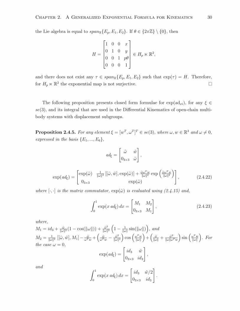
Chapter 2. A Generalized Exponential Formula for Kinematics 30
the Lie algebra is equal to spanREp, E1, E2. If θ ∈ 2πZ \ 0, then
H =
1 0 0 x
0 1 0 y
0 0 1 pθ
0 0 0 1
∈ Hp nR2,
and there does not exist any τ ∈ spanREp, E1, E2 such that exp(τ) = H. Therefore,
for Hp nR2 the exponential map is not surjective.
The following proposition presents closed form formulae for exp(adxi), for any ξ ∈se(3), and its integral that are used in the Differential Kinematics of open-chain multi-
body systems with displacement subgroups.
Proposition 2.4.5. For any element ξ = [wT , ωT ]T ∈ se(3), where ω,w ∈ R3 and ω 6= 0,
expressed in the basis E1, ..., E6,
adξ =
[ω w
03×3 ω
],
exp(adξ) =
[exp(ω) 1
‖ω‖2 [[ω, w], exp(ω)] + ωωTw‖ω‖2 exp
(ωωTw‖ω‖2
)03×3 exp(ω)
], (2.4.22)
where [·, ·] is the matrix commutator, exp(ω) is evaluated using (2.4.15) and,
∫ 1
0
exp(x adξ) dx =
[M1 M2
03×3 M1
], (2.4.23)
where,
M1 = id3 + ω‖ω‖2 (1− cos(‖ω‖)) + ω2
‖ω‖2
(1− 1
‖ω‖ sin(‖ω‖))
, and
M2 = 1‖ω‖2 [[ω, w],M1]− ω
ωTw+(
ωωTw− ω2
‖ω‖2
)cos(ωTw‖ω‖
)+(
ω‖ω‖ + ω2
‖ω‖ωTw
)sin(ωTw‖ω‖
). For
the case ω = 0,
exp(adξ) =
[id3 w
03×3 id3
],
and ∫ 1
0
exp(x adξ) dx =
[id3 w/2
03×3 id3
].

Chapter 2. A Generalized Exponential Formula for Kinematics 31
Proof. Case 1) When ω = 0,
adξ =
[03×3 w
03×3 03×3
].
Using the Taylor expansion of the matrix exponential, exp(adξ) =∑∞
i=0
(adiξ/i!
), and
the fact that adξ is nilpotent of degree two, i.e., adiξ = 0 for i ≥ 2, it is easy to show the
result.
Case 2) To prove the result for ω 6= 0, the following lemma is required.
Lemma 2.4.6. ∀ω,w ∈ R3 and ω ∈ so(3),
(i) ω2 = ωωT − ‖ω‖2id3 [57],
(ii) ω3 = −‖ω‖2ω [57],
(iii) ωw = −wω = ω × w,
(iv) ˜ωw = [ω, w].
The proof for the above lemma is a straight forward computation. Now, consider the
Adjoint operator corresponding to the element H, AdH , for
H =
[id3
−ωw‖ω‖2
01×3 1
]∈ SE(3),
and its action on ξ ∈ se(3). Based on Lemma 2.4.6,
ξ′ : = AdHξ =
[id3 − [ω,w]
‖ω‖2
03×3 id3
][w
ω
]=
[w − ωw ω
‖ω‖2 + wω ω‖ω‖2
ω
]
=
[w +
(ωωT − ‖ω‖2id3
)w‖ω‖2
ω
]=
[(ωTw)ω‖ω‖2
ω
]=:
[hω
ω
].
Hence,
exp(adξ′) =∞∑i=0
adiξ′
i!=
∞∑i=0
1
i!
[ωi i(hω)i
03×3 ωi
]=
[exp(ω)
∑∞i=1
(hω)i
(i−1)!
03×3 exp(ω)
]
=
[exp(ω) ∂
∂µ|µ=1 exp(hωµ)
03×3 exp(ω)
]=
[exp(ω) hω exp(hω)
03×3 exp(ω)
].

Chapter 2. A Generalized Exponential Formula for Kinematics 32
According to the definition of the adjoint operator, one has the following:
exp(adξ) = exp(adAdH−1 (ξ′)) = Adexp(AdH−1 (ξ′)) = Ad(H−1 exp(ξ′)H) = AdH−1 exp(adξ′)AdH .
A straightforward calculation proves the first part of the proposition. For the second
part of the proposition,∫ 1
0
exp(x adξ) dx
=
∫ 1
0
[exp(xω) 1
x2‖ω‖2 [[xω, xw], exp(xω)] + xhω exp(xhω)
03×3 exp(xω)
]dx.
Since the matrix commutator is a bilinear operator, and the integral operator and partial
derivative can commute,∫ 1
0
exp(x adξ) dx
=
[∫ 1
0exp(xω) dx 1
‖ω‖2
[[ω, w],
∫ 1
0exp(xω) dx
]+∫ 1
0xhω exp(xhω) dx
03×3
∫ 1
0exp(xω) dx
].
Using (2.4.15) and substituting h = ωTw‖ω‖2 , one can show the second part of the proposition.
2.5 Case Study
In this section, the kinematic analysis of a mobile manipulator moving on a spacecraft
is performed to elaborate the computational aspects of the proposed formulation for
Forward and Differential Kinematics of open-chain multi-body systems. The spacecraft
can be considered as a six-d.o.f. moving base for the mobile manipulator that is shown
in Figure 2.1. The multi-body system MS(6) = (Bi, Ai)|i = 0, ..., 6, Bi ⊂ Ai consists
of two branches and six joints. The first branch consists of B0 to B5. The second branch
contains B6 and joint six is its last joint. Joint one is a free joint, the second joint is
a nonholonomic three-d.o.f. planar joint, the next joint is a three-d.o.f. spherical joint
and the rest of the joints are one-d.o.f. revolute joints. The coordinate frames assigned
to A0, ..., A6 at the initial configuration are shown in Figure 2.2. In the sequel, the joint
parameters are specified, and Forward and Differential Kinematics maps of MS(6) are
determined. Note that in the following, a basis for Vj at the initial configuration is denoted

Chapter 2. A Generalized Exponential Formula for Kinematics 33
Figure 2.1: A mobile manipulator on a six d.o.f. moving base
by Xj, Yj, Zj, and the linear operator 0τ j−1j in the chosen coordinates is represented by
the matrix 0T j−1j .
2.5.1 Forward Kinematics
The first joint is a six-d.o.f. holonomic joint between B0 and B1. The classic joint pa-
rameters are q1 = [x1, y1, z1, θ1,x, θ1,y, θ1,z]T , where [x1, y1, z1]T is the position of H0
1 (t)(O1)
with respect to H01,0(O1) and expressed in V0, and [θ1,x, θ1,y, θ1,z]
T is the rotation angles
of V1 with respect to the axes of V1 at the initial configuration. Therefore, the local
coordinate chart ϕ1 for Q1 is
ϕ1(q1) =
[R(θ1,x, X1)R(θ1,y, Y1)R(θ1,z, Z1) [x1, y1, z1]T
01×3 1
],
where R(θ, W ) is the 3 × 3 rotation matrix corresponding to θ radian rotation about
the vector W . For this coordinate chart, any element of Lie(P0) corresponding to the
relative pose of B1 with respect to B0 is parametrized with the screw joint parameters
s1 = [s1,1, ..., s1,6]T , such that
0T 01 s1 =
(AdH0
1,0
)(Tid6ι1) (T0ϕ1) s1.
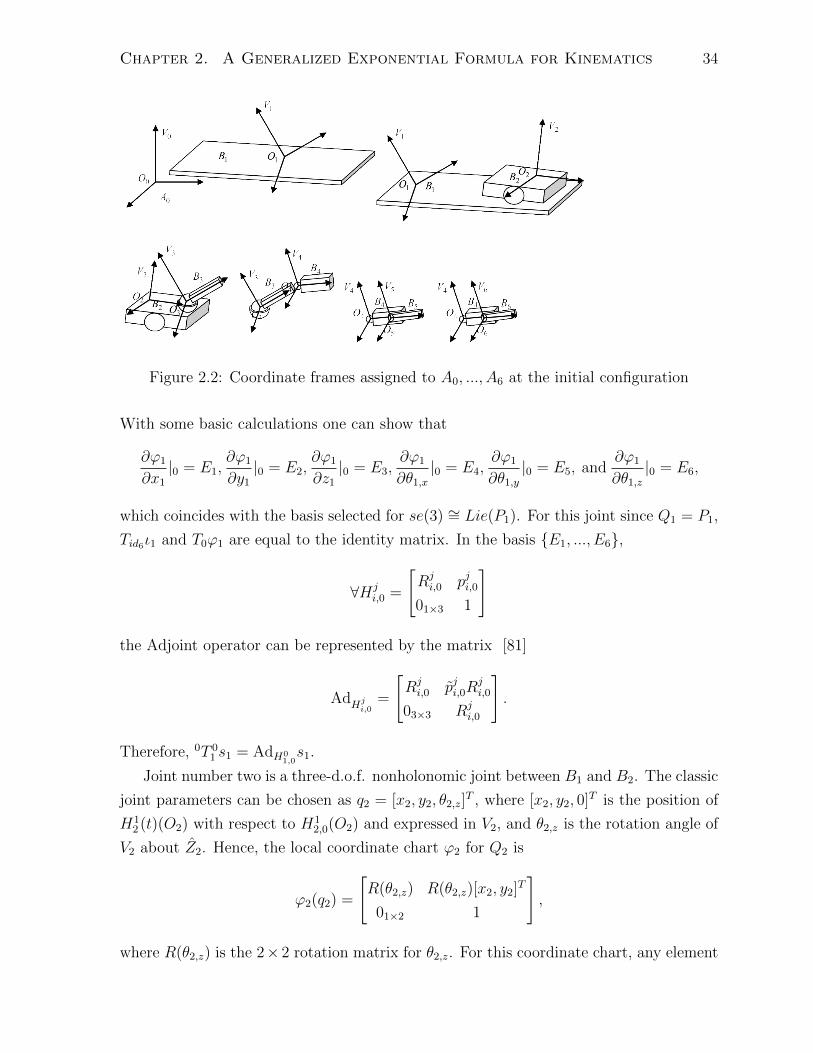
Chapter 2. A Generalized Exponential Formula for Kinematics 34
Figure 2.2: Coordinate frames assigned to A0, ..., A6 at the initial configuration
With some basic calculations one can show that
∂ϕ1
∂x1
|0 = E1,∂ϕ1
∂y1
|0 = E2,∂ϕ1
∂z1
|0 = E3,∂ϕ1
∂θ1,x
|0 = E4,∂ϕ1
∂θ1,y
|0 = E5, and∂ϕ1
∂θ1,z
|0 = E6,
which coincides with the basis selected for se(3) ∼= Lie(P1). For this joint since Q1 = P1,
Tid6ι1 and T0ϕ1 are equal to the identity matrix. In the basis E1, ..., E6,
∀Hji,0 =
[Rji,0 pji,0
01×3 1
]
the Adjoint operator can be represented by the matrix [81]
AdHji,0
=
[Rji,0 pji,0R
ji,0
03×3 Rji,0
].
Therefore, 0T 01 s1 = AdH0
1,0s1.
Joint number two is a three-d.o.f. nonholonomic joint between B1 and B2. The classic
joint parameters can be chosen as q2 = [x2, y2, θ2,z]T , where [x2, y2, 0]T is the position of
H12 (t)(O2) with respect to H1
2,0(O2) and expressed in V2, and θ2,z is the rotation angle of
V2 about Z2. Hence, the local coordinate chart ϕ2 for Q2 is
ϕ2(q2) =
[R(θ2,z) R(θ2,z)[x2, y2]T
01×2 1
],
where R(θ2,z) is the 2× 2 rotation matrix for θ2,z. For this coordinate chart, any element

Chapter 2. A Generalized Exponential Formula for Kinematics 35
of Lie(P0) corresponding to the relative pose of B2 with respect to B1 is parametrized
by the screw joint parameters s2 = [s2,1, s2,2, s2,3]T , such that
0T 12 s2 =
(AdH1
2,0
)(Tid3ι2) (T0ϕ2) s2,
where
Tid3ι2∂ϕ2
∂x2
|0 = E1, Tid3ι2∂ϕ2
∂y2
|0 = E2, and Tid3ι2∂ϕ2
∂θ2,z
|0 = E6.
Thus,
0T 12 s2 = AdH0
2,0
1 0 · · · 0
0 1 · · · 0
0 0 · · · 1
T
s2.
The third joint is a three-d.o.f. holonomic joint between B2 and B3. The classic joint
parameters are q3 = [θ3,x, θ3,y, θ3,z]T , and the local coordinate chart for Q3 is ϕ3(q3) =
R(θ3,x, X3)R(θ3,y, Y3)R(θ3,z, Z3). The elements of Lie(P0) corresponding to the relative
poses of B3 with respect to B2 are parametrized by the screw joint parameters s3 =
[s3,1, s3,2, s3,3]T , such that
0T 23 s3 = AdH0
3,0
[03×3
id3
]s3.
Joint 4 is a one-d.o.f. revolute joint, its classic joint parameter is q4 = θ4,z, and the
local coordinate chart for Q4 is ϕ4(q4) = R(θ4,z).The line in Lie(P0) corresponding to the
relative pose of B4 with respect to B5 is parametrized by the screw joint parameter s4,
such that0T 3
4 s4 = AdH04,0
[0, ..., 1]T s4.
By a simple calculation
0T 34 =
[p0
4,0 ×0 Z4
0Z4
],
where 0Z4 is the joint screw axis expressed in V0. Hence, 0T 34 s4 coincides with the
argument of the exponential map in the existing product of exponentials formula for a
revolute joint [11, 57, 71]. Similarly, for the fifth and sixth joints
0T 45 s5 = AdH0
5,0[0, ..., 1]T s5,
0T 46 s6 = AdH0
6,0[0, ..., 1]T s6,
respectively.
Therefore, based on (2.2.6), the Forward Kinematics map corresponding to MS(6) is

Chapter 2. A Generalized Exponential Formula for Kinematics 36
FK(s) =
[exp(0T 0
1 s1)... exp(0T 45 s5)H0
5,0
exp(0T 01 s1)... exp(0T 4
6 s6)H06,0
],
where exp is the matrix exponential for SE(3) that can be evaluated by (2.4.14) and
s = [sT1 , ..., vT6 ]T .
According to the calculation performed in the case of joint four, for a serial-link
multi-body system with revolute and/or prismatic joints, where the multi-body system
consists of one branch, the above formulation for FK reduces to the existing product of
exponentials formula.
2.5.2 Differential Kinematics
Based on Proposition 2.4.1 and 2.4.5, the Jacobian maps of B5 and B6 with respect to B0
and expressed in V0, i.e., 0J05 (s) and 0J0
6 (s), can be determined as 6× 14 matrices. The
nonholonomic constraints at the second joint can be expressed in terms of the classical
joint parameters as
C2(q2)q2 = [0, 1, 0]q2 = 0,
which indicates that the mobile base cannot drift side way. The annihilator of C2 can be
selected to be
C2(q2) =
[1 0 0
0 0 1
]T,
and therefore using (2.1.3b) and (2.1.5)
Σ2(s2) =
sin(s2,3)
s2,3s2,2
(cos(s2,3)+s2,3 sin(s2,3)−1)
s22,3+ s2,1
(cos(s2,3)+sin(s2,3)/s2,3)
s2,3(cos(s2,3)−1)
s2,3s2,1
(1−cos(s2,3)−s2,3 sin(s2,3))
s22,3+ s2,2
(cos(s2,3)−sin(s2,3)/s2,3)
s2,3
0 1
.Note that when s2,3 = 0,
Σ2(s2) =
[1 0 0
s2,2/2 −s2,1/2 1
]T.
Finally, according to (2.3.13) the modified Jacobian of the multi-body system MS(6)
becomes
J(s) =
[0J0
5 (s) 06×13
06×130J0
6 (s)
],
Chapter 2. A Generalized Exponential Formula for Kinematics 37
which can be calculated as a 12× 26 matrix using Proposition 2.4.1 and 2.4.5.

Chapter 3
Symplectic Reduction of Holonomic
Open-chain Multi-body Systems
with Displacement Subgroups
This Chapter presents a symplectic geometric approach to the reduction of Hamilton’s
equation for holonomic open-chain multi-body systems with multi-degree-of-freedom dis-
placement subgroups.
First in Section 3.1, we revisit Hamilton’s principle for Lagrangian systems, and we
use the Hamilton-Pontryagin principle to study the geometry of Hamiltonian systems. In
Section 3.2 we use the symplectic reduction theorem to express Hamilton’s equation in
the symplectic reduced manifold, for holonomic Hamiltonian mechanical systems. Then
by identifying the symplectic reduced manifold with a cotangent bundle, we express the
reduced Hamilton’s equation in that cotangent bundle. Consequently, in Section 3.3
we apply this procedure to open-chain multi-body systems with multi-degree-of-freedom
displacement subgroups, for which the symmetry group is identified with the configura-
tion manifold corresponding to the first joint. Then we derive their reduced dynamical
equations in local coordinates, in Theorem 3.3.6.
3.1 Hamilton-Pontryagin Principle and Hamilton’s
Equation
In this section we first explore the geometry of Hamilton’s principle for Lagrangian sys-
tems. Then we show how this principle leads to the Hamilton-Pontryagin principle on
the Pontryagin bundle TQ ⊕ T ∗Q. The Lagrangian systems that satisfy the Hamilton-
38

Chapter 3. Reduction of Holonomic Multi-body Systems 39
Pontryagin principle are called implicit Lagrangian systems, and the resulting equation of
motion is called the implicit Euler-Lagrange equation [93, 94]. In addition, we show that
for hyper-regular Lagrangian systems the implicit Euler-Lagrange equation is equivalent
to Hamilton’s equation. In the next chapter, we use an analogous method to derive the
equations of motion for nonholonomic systems, using Lagrange-d’Alembert-Pontryagin
principle.
Let TQ be the tangent bundle of the configuration manifold Q, and let L : TQ → Rbe a smooth function; we call L the Lagrangian. Let t 7→ vq(t)(t) ∈ Tq(t)Q be a smooth
curve in TQ. This curve corresponds to a tangent lift of a curve in Q if vq(t)(t) = dqdt
(t) =:
qq(t)(t), ∀t. For a time interval [ts, tf ], let (t, ε) 7→ q(t, ε) ∈ Q, for ε ∈ R, be a variation
of a smooth curve t 7→ q(t) ∈ Q with fixed end points qs, qf ∈ Q, i.e., q(ts, ε) = qs and
q(tf , ε) = qf , along with the condition that q(t, 0) = q(t). Hamilton’s principle states that
a Lagrangian system evolves on a curve t 7→ vq(t)(t) that is the tangent lift of the curve
t 7→ q(t) and that makes the action functional stationary for any arbitrary variation of
the curve t 7→ q(t) with fixed end points. That is,
∂
∂ε
∣∣∣∣ε=0
∫ tf
ts
L(vq(t,ε)(t, ε))dt = 0 (3.1.1)
for any variation as described above. This holds if and only if the curve t 7→ vq(t)(t)
satisfies the Euler-Lagrange equation, which is written in coordinates as
d
dt(∂L
∂q(qq(t)(t)))−
∂L
∂q(qq(t)(t)) = 0. (3.1.2)
We present the Euler-Lagrange equation (and upcoming dynamical equations) in the
form of paired elements of cotangent and tangent bundles, for the sake of generalizing
them to nonholonomic systems in the next chapter:⟨(d
dt(∂L
∂q(qq(t)(t)))−
∂L
∂q(qq(t)(t))
)dq, wq(t)
⟩= 0,
∀t ∈ (ts, tf ) and ∀wq(t) ∈ Tq(t)Q,
As was mentioned above, in Hamilton’s principle the variational problem deals only
with tangent lifted curves in TQ. One may implicitly impose this kinematic constraint
in the variational problem, and form a variational problem in the Pontryagin bundle
PQ := TQ ⊕ T ∗Q. The Pontryagin bundle is a vector bundle over the configuration
manifold Q with the canonical projection ΠQ : PQ → Q such that ∀vq ∈ TqQ and
∀pq ∈ T ∗qQ we write (vq, pq) ∈ PqQ and we have ΠQ(vq, pq) = q. The resulting equivalent

Chapter 3. Reduction of Holonomic Multi-body Systems 40
principle is called Hamilton-Pontryagin principle. This principle states that an implicit
Lagrangian system evolves on a curve t 7→ (vq(t)(t), pq(t)(t)) ∈ Pq(t)Q that makes the
following functional stationary for any arbitrary variation of the curve in PQ with fixed
end points in Q, i.e., q(ts, ε) = qs and q(tf , ε) = qf :
∂
∂ε
∣∣∣∣ε=0
∫ tf
ts
(L(vq(t,ε)(t, ε)) +
⟨pq(t,ε)(t, ε), qq(t,ε)(t, ε)− vq(t,ε)(t, ε)
⟩)dt = 0. (3.1.3)
For the time interval [ts, tf ], we denote any variation of the curve t 7→ (vq(t)(t), pq(t)(t)) ∈Pq(t)Q by a function γ : [ts, tf ]× R→ PQ:
γ(t, ε) = (vq(t,ε)(t, ε), pq(t,ε)(t, ε)).
For γ to be a variation with fixed end points in Q we assume that for all ε ∈ R,
ΠQ(γ(ts, ε)) = qs and ΠQ(γ(tf , ε)) = qf . We denote the induced map by ΠQ on the
tangent bundles by TΠQ : TPQ → TQ and the projection map that projects the Pon-
tryagin bundle onto T ∗Q by ΠT ∗Q : PQ → T ∗Q. Let Θcan and Ωcan := −dΘcan be the
tautological 1-form and the canonical 2-form on T ∗Q, and let γ := ∂γ∂t∈ Tγ(t,ε)(PQ) and
δγ := ∂γ∂ε
∣∣ε=0∈ Tγ(t,0)(PQ). We can write the left hand side of (3.1.3) as
∂
∂ε
∣∣∣∣ε=0
∫ tf
ts
(L(vq) + 〈pq, TΠQ(γ)− vq〉) γ dt
=
∫ tf
ts
(〈(dL− d〈pq, vq〉) γ(t, 0), δγ(t)〉+
∂
∂ε
∣∣∣∣ε=0
〈(T ∗ΠT ∗Q(Θcan)) γ, γ〉)dt
=
∫ tf
ts
∂
∂t〈(T ∗ΠT ∗QΘcan) γ(t, 0), δγ(t)〉 dt
+
∫ tf
ts
⟨(dL− d〈pq, vq〉) γ(t, 0) + ιγ(t,0) ((T ∗ΠT ∗QΩcan) γ(t, 0)) , δγ(t)
⟩dt
(by Lemma 3.1.1 bellow)
= [〈(T ∗ΠT ∗QΘcan) γ(t, 0), δγ(t)〉]tfts
+
∫ tf
ts
⟨(dL− d〈pq, vq〉) γ(t, 0) + ιγ(t,0) ((T ∗ΠT ∗QΩcan) γ(t, 0)) , δγ(t)
⟩dt
=
∫ tf
ts
⟨(dL− d〈pq, vq〉) γ(t, 0) + ιγ(t,0) ((T ∗ΠT ∗QΩcan) γ(t, 0)) , δγ(t)
⟩dt
(since the variation in Q at the end points is zero)
In the above calculation, the first equality follows from the definition of the tautological

Chapter 3. Reduction of Holonomic Multi-body Systems 41
1-form Θcan ∈ Ω1(T ∗Q) and from the following diagram:
PQΠT∗Q //
ΠQ
T ∗Q
πQ
Q Q
where πQ : T ∗Q → Q is the canonical projection of the cotangent bundle. Since δγ(t) ∈Tγ(t,0)PQ is arbitrary, we can write (3.1.3) as, ∀Wγ(t,0) ∈ Tγ(t,0)(PQ),
⟨d(L− 〈pq, vq〉) γ(t, 0) + ιγ(t,0) ((T ∗ΠT ∗QΩcan) γ(t, 0)) ,Wγ(t,0)
⟩= 0,
or equivalently,
d(L− 〈pq, vq〉) γ(t, 0) + ιγ(t,0) ((T ∗ΠT ∗QΩcan) γ(t, 0)) = 0. (3.1.4)
The 2-form T ∗ΠT ∗QΩcan is a closed degenerate 2-form on PQ. It is degenerate only
in the direction of vq, that is, ∀(vq, pq) ∈ PqQ and ∀W(vq ,pq) ∈ T(vq ,pq)(PQ), we have
ιW(T ∗ΠT ∗QΩcan) = 0 if and only if T(vq ,pq)ΠT ∗Q(W(vq ,pq)) = 0.
Lemma 3.1.1. For any variation γ as described above and for all α ∈ Ω1(PQ), we have
the equality
∂
∂ε
∣∣∣∣ε=0
〈α γ(t, ε), γ(t, ε)〉 =∂
∂t〈α γ(t, 0), δγ(t)〉+ 〈ιγ(t,0)(−dα γ(t, 0)), δγ(t)〉.
Proof. The proof is based on a straightforward calculation.
∂
∂ε〈α γ(t, ε), γ(t, ε)〉 =
∂
∂ε
⟨α γ, Tγ(
∂
∂t)
⟩= L∂/∂ε
⟨T ∗γ(α),
∂
∂t
⟩=
⟨L∂/∂ε(T ∗γ(α)),
∂
∂t
⟩+
⟨T ∗γ(α),L∂/∂ε(
∂
∂t)
⟩=
⟨L∂/∂ε(T ∗γ(α)),
∂
∂t
⟩(t and ε are two independent variables)
=
⟨ι∂/∂ε(T
∗γ(dα)) + d
⟨T ∗γ(α),
∂
∂ε
⟩,∂
∂t
⟩(by Cartan’s formula)
=
⟨−ι∂/∂t(T ∗γ(dα)),
∂
∂ε
⟩+∂
∂t
⟨T ∗γ(α),
∂
∂ε
⟩

Chapter 3. Reduction of Holonomic Multi-body Systems 42
=
⟨T ∗γ (ιγ(−dα γ)) ,
∂
∂ε
⟩+∂
∂t
⟨T ∗γ(α),
∂
∂ε
⟩=
⟨ιγ(−dα γ), Tγ(
∂
∂ε)
⟩+∂
∂t
⟨α γ, Tγ(
∂
∂ε)
⟩Based on the definition of δγ(t), at ε = 0 we have the desired equality.
We define the function E : PQ → R by E(vq, pq) := 〈pq, vq〉 − L(vq); it is called
the energy function. We call the triple (PQ, T ∗ΠT ∗QΩcan ∈ Ω2(PQ), E) an implicit
Lagrangian system.
In a coordinate chart, we have (γ(t, 0), γ(t, 0)) = (q(t), v(t), p(t), q(t), v(t), p(t)) and
T ∗ΠT ∗QΩcan = −dp ∧ dq. We can write (3.1.4) as
∂L
∂q(q, v)dq +
∂L
∂v(q, v)dv + qdp− pdq − vdp− pdv = 0,
or equivalently,
p =∂L
∂q(q, v), p =
∂L
∂v(q, v), q = v. (3.1.5)
This gives a bijection between the tangent lift of the curves in Q that satisfy the Euler-
Lagrange equation (3.1.2) and the curves in PQ that satisfy the implicit Euler-Lagrange
equation (3.1.5).
The fibre derivative of the Lagrangian L induces a fibre preserving map FL : TQ →T ∗Q, called Legendre transformation,
〈FLq(vq), wq〉 :=d
dε
∣∣∣∣ε=0
L(vq + εwq) =
⟨∂L
∂v(vq), wq
⟩. ∀wq ∈ TqQ (3.1.6)
For all vq ∈ TqQ we can define the embedding grph : TQ → PQ by grphq(vq) :=
(vq,FLq(vq)) ∈ PqQ. By (3.1.5), we have that the solution curve of an implicit La-
grangian system is always in this submanifold.
The Lagrangian L is called hyper-regular if FL is a diffeomorphism. Under the
assumption that L is hyper-regular, we also have the embedding grph : T ∗Q → PQthat maps any element pq ∈ T ∗Q to (FL−1(pq), pq) ∈ PqQ. In this case, we have
grph(T ∗Q) = grph(TQ); hence in (3.1.4) the curve t 7→ γ(t, 0) is in the image of grph,
and it has a unique pre-image t 7→ λ(t) = pq(t)(t) ∈ T ∗q(t)Q, such that λ(t) = ΠT ∗Q(γ(t, 0)),
for all t. Assuming that L is hyper-regular, we can now rewrite (3.1.4) in T ∗Q as
T ∗grph(ιγ(t,0) ((T ∗ΠT ∗QΩcan) γ(t, 0))− dE γ(t, 0)
)= 0,

Chapter 3. Reduction of Holonomic Multi-body Systems 43
⇐⇒ ιλ(t) (Ωcan λ(t))− dE grph(λ(t)) = 0,
since we have the following diagram:
T ∗Q
T ∗Q grph // PQ
ΠT∗Q
OO
Here, λ(t) := dλdt
(t). We define the Hamiltonian function H : T ∗Q → R on the cotangent
bundle by
H(pq) := E grph(pq) = 〈pq,FL−1(pq)〉 − L(FL−1(pq)). (3.1.7)
For a hyper-regular Lagrangian, the solution curve of an implicit Lagrangian system, i.e.,
t 7→ γ(t, 0), satisfies (3.1.4) if and only if the curve t 7→ λ(t) satisfies Hamilton’s equation,
defined by
ιλ(t) (Ωcan λ(t)) = dH λ(t). (3.1.8)
Let πQ : T ∗Q → Q be the canonical projection map for the cotangent bundle, and
(with some abuse of notation) denote a variation of the curve t 7→ λ(t) ∈ T ∗Q by the
function (t, ε) 7→ λ(t, ε) ∈ T ∗Q. Under the assumptions considered to derive (3.1.4),
Hamilton’s equation in T ∗Q can also be derived from the Hamilton-Pontryagin principle,
once we restrict the variational problem to the image of the embedding grph. That is, we
only consider the variations (t, ε) 7→ γ(t, ε) ∈ grph(T ∗Q) such that λ(t, ε) = ΠT ∗Q(γ(t, ε)):
∂
∂ε
∣∣∣∣ε=0
∫ tf
ts
(L(vq) + 〈pq, TΠQ(γ)− vq〉) γ dt = 0
⇐⇒ ∂
∂ε
∣∣∣∣ε=0
∫ tf
ts
(〈λ(t, ε), TπQ(λ(t, ε))〉 −H λ(t, ε))
)dt = 0
⇐⇒⟨ιλ(t,0) (Ωcan λ(t, 0))− dH λ(t, 0), δλ(t)
⟩= 0, ∀δλ(t) ∈ Tλ(t,0)(T
∗Q)
⇐⇒ ιλ(t) (Ωcan λ(t)) = dH λ(t).
Here, λ(t, ε) := ∂∂tλ(t, ε) and δλ(t) := ∂
∂ε
∣∣ε=0
λ(t, ε). Note that the details are omitted
here, since the derivation presented above is similar to the derivation of (3.1.4).
Using any coordinate chart for T ∗Q, we have (λ(t), λ(t)) = (q(t), p(t), q(t), p(t)), and

Chapter 3. Reduction of Holonomic Multi-body Systems 44
we can write (3.1.8) as
q =∂H
∂p, p = −∂H
∂q.
Now, let X be a vector field on the cotangent bundle T ∗Q. It induces a vector field
on grph(T ∗Q) whose smooth extension to PQ is denoted by X . Note that X is not a
unique vector field on PQ. In other words, ∀pq ∈ T ∗Q we have Tpq grph(Xpq) = Xgrph(pq).
If the curve t 7→ γ(t) ∈ PQ is an integral curve of the vector field X and it satisfies
(3.1.4), then ∀Wγ(t) ∈ Tγ(t)(PQ) we have
⟨(−dE + ιX (T ∗ΠT ∗QΩcan)) γ(t),Wγ(t)
⟩= 0,
⇐⇒ (−dE + ιX (T ∗ΠT ∗QΩcan)) γ(t) = 0. (3.1.9)
It is easy to show that the pull back of the 1-form ιX (T ∗ΠT ∗QΩcan) − dE ∈ Ω1(PQ)
(restricted to the image of grph) by the embedding grph is equal to
ιXΩcan − dH ∈ Ω1(T ∗Q).
Consequently, any curve t 7→ γ(t) ∈ grph(T ∗Q) such that Xγ(t) = dγdt
(t) satisfies (3.1.9) if
and only if the curve t 7→ λ(t) = ΠT ∗Q(γ(t)) ∈ T ∗Q, which is the integral curve of the
vector field X, satisfies
⟨(ιXΩcan − dH) λ(t),Yλ(t)
⟩= 0, ∀Yλ(t) ∈ Tλ(t)(T
∗Q)
⇐⇒ (ιXΩcan − dH) λ(t) = 0. (3.1.10)
If (3.1.10) holds for any integral curve of X ∈ X(T ∗Q), we can define Hamilton’s
equation as
ιXΩcan = dH. (3.1.11)
In general, one can have a system satisfying Hamilton’s equation (3.1.11) on T ∗Q for a
Hamiltonian H ∈ C∞(T ∗Q) that does not necessarily come from a Lagrangian. Such
system is called a Hamiltonian system. The unique vector field that satisfies Hamilton’s
equation for a Hamiltonian H is called the Hamiltonian vector field for the Hamiltonian
H. We define a Hamiltonian system to be a triple (T ∗Q,Ωcan, H), as above.

Chapter 3. Reduction of Holonomic Multi-body Systems 45
3.2 Hamiltonian Mechanical Systems with Symme-
try
For a mechanical system, the Lagrangian is defined by L := 12Kq(vq, vq) − V (q), where
Kq : TqQ×TqQ → R is a Riemannian metric, called the kinetic energy metric, and where
V : Q → R is a smooth function, called the potential energy function. This Lagrangian is
hyper-regular, and the corresponding Legendre transformation is equal to the fibre-wise
linear isomorphism that is induced by the metric K:
〈FLq(vq), wq〉 := Kq(vq, wq). ∀vq, wq ∈ TqQ (3.2.12)
Likewise, the Hamiltonian of the system is
H(pq) =1
2Kq(FL−1
q (pq),FL−1q (pq)) + V (q), (3.2.13)
which is the total energy of the mechanical system. A Hamiltonian mechanical system is
such a quadruple (T ∗Q,Ωcan, H,K).
Let G be a Lie group with the Lie algebra Lie(G). Consider an action of G on Q, and
denote the action by Φg : Q → Q, ∀g ∈ G. This action induces an action of G on T ∗Qby the cotangent lift of Φg, which is denoted by T ∗Φg : T ∗Q → T ∗Q.
Lemma 3.2.1. For every g ∈ G, the map T ∗Φg is a symplectomorphism, i.e., it preserves
Ωcan [50].
Proof. The proof relies on the fact that T ∗Φg preserves the tautological 1-form Θcan:
⟨(T ∗T ∗Φg(Θcan))pq ,Ypq
⟩=⟨T ∗Φg(pq), (TπQ)(TT ∗Φg)(Ypq)
⟩= ∀Ypq ∈ Tpq(T ∗Q)⟨
T ∗Φg(pq), T (πQ T ∗Φg)(Ypq)⟩
=⟨T ∗Φg(pq), T (Φg−1 πQ)(Ypq)
⟩=⟨
pq, TπQ(Ypq)⟩
=⟨(Θcan)pq ,Ypq
⟩.
The third equality holds, since the following diagram commutes:
T ∗Q
πQ
T ∗Φg // T ∗Q
πQ
Q
Φg−1// Q

Chapter 3. Reduction of Holonomic Multi-body Systems 46
Finally, we have
T ∗T ∗Φg(Ωcan) = T ∗T ∗Φg(−dΘcan) = −d (T ∗T ∗Φg(Θcan)) = −dΘcan = Ωcan.
Consider the infinitesimal action of Lie(G) on Q. For any ξ ∈ Lie(G), this action
induces a vector field ξQ ∈ X(Q) such that ∀q ∈ Q,
ξQ(q) =∂
∂ε
∣∣∣∣ε=0
(Φexp(εξ)(q)
). (3.2.14)
Denote the fibre-wise linear map corresponding to the infinitesimal action of Lie(G) by
φq : Lie(G) → TqQ, where φq(ξ) = ξQ(q). Likewise, we define ξT ∗Q ∈ X(T ∗Q) such that
∀pq ∈ T ∗qQ,
ξT ∗Q(pq) =∂
∂ε
∣∣∣∣ε=0
(T ∗Φexp(εξ)(q)
Φexp(−εξ)(pq)). (3.2.15)
Now, consider the fibre-wise linear map M : T ∗Q → Lie∗(G), defined by
〈Mq(pq), ξ〉 := 〈φ∗q(pq), ξ〉 = 〈pq, ξQ(q)〉. (3.2.16)
Lemma 3.2.2. The map M is an Ad∗-equivariant momentum map corresponding to the
cotangent lifted action T ∗Φg.
Proof. To prove that M is a momentum map, it suffices to show that M satisfies the
momentum equation (1.2.1) for the G-action on T ∗Q,
ιξT∗QΩcan = d〈M, ξ〉.
Therefore, we have
d〈M(pq), ξ〉 = d〈pq, ξQ〉 = d(ιξT∗QΘcan
)= LξT∗QΘcan − ιξT∗QdΘcan = ιξT∗QΩcan.
The forth equality is true, since the cotangent lifted action preserves the tautological
1-form.
To prove that M is Ad∗-equivariant, we have to show
M(T ∗Φg(pq)) = Ad∗gM(pq).

Chapter 3. Reduction of Holonomic Multi-body Systems 47
Using the definition of action and the map M, ∀ξ ∈ Lie(G) one has
〈M(T ∗Φg(pq)), ξ〉 = 〈T ∗Φg(pq), ξQ(Φg−1(q))〉 = 〈pq,∂
∂ε
∣∣∣∣ε=0
(Φg exp(εξ)g−1(q)
)〉 =
〈pq, (Adgξ)Q(q))〉 = 〈Ad∗gM(pq), ξ〉.
Proposition 3.2.3 (Noether’s Theorem). Let H : T ∗Q → R be the Hamiltonian of a
mechanical system. If H is invariant under the cotangent lifted group action, the mo-
mentum map M is constant along the flow of the Hamiltonian vector field X for the
Hamiltonian H. That is, ∀ξ ∈ Lie(G) we have LX(〈M, ξ〉) = 0.
Proof.
LX(〈M, ξ〉) = 〈d〈M, ξ〉, X〉 =⟨ιξT∗QΩcan, X
⟩= −Ωcan(X, ξT ∗Q) = −〈ιXΩcan, ξT ∗Q〉 =
− 〈dH, ξT ∗Q〉 = −LξT∗QH = 0.
The forth equality is true, since X is a Hamiltonian vector field for the function H, and
the last equality is the consequence of the hypothesis that H is G-invariant.
We define a Hamiltonian system with symmetry to be a quadruple (T ∗Q,Ωcan, H,G),
as above, where the Hamiltonian H is invariant under the cotangent lifted action of G. A
Hamiltonian mechanical system with symmetry is defined by a quintuple (T ∗Q,Ωcan, H,K,G),
where K is the kinetic energy metric on Q, and in addition to H, K is invariant under
the G-action.
Theorem 3.2.4 (Symplectic Reduction Theorem [53]). Assume that the action of G on
Q is free and proper, and let µ ∈ Lie∗(G) be a regular value of its momentum map M.
Also, let Gµ = g ∈ G|Ad∗gµ = µ be the coadjoint isotropy group for µ ∈ Lie∗(G).
Then the quotient manifold (T ∗Q)µ := M−1(µ)/Gµ is a symplectic manifold, called
the symplectic reduced space, with the unique symplectic form Ωµ that is identified by
the equality T ∗πµ(Ωµ) = T ∗iµ(Ωcan). Here, the maps πµ : M−1(µ) → M−1(µ)/Gµ and
iµ : M−1(µ) → T ∗Q are the projection map and inclusion map, respectively.
This theorem was first stated and proved in a paper by Marsden and Weinstein in
1974 [53], and since then this result has been extended to non-free actions [27] and almost
symplectic manifolds [39]. An almost symplectic manifold is a manifold equipped with
a nondegenerate 2-form, which may not be closed. Based on the symplectic reduction

Chapter 3. Reduction of Holonomic Multi-body Systems 48
theorem, in the presence of a group action that preserves the symplectic structure and
an Ad∗-equivariant momentum map (corresponding to the symmetry group) we say that
the phase space of a Hamiltonian system along with its symplectic 2-form can be reduced
to the symplectic reduced space ((T ∗Q)µ,Ωµ). In order to have a well-defined projection
of Hamilton’s equation onto the symplectic reduced space, the Hamiltonian of the system
should be invariant under the group action, as well. Under these hypotheses, Hamilton’s
equation can be written on (T ∗Q)µ as
ιXµΩµ = dHµ, (3.2.17)
where Hµ is defined by H iµ = Hµ πµ and Xµ πµ = Tπµ(X iµ).
We say that the Hamiltonian system with symmetry (T ∗Q,Ωcan, H,G) has been re-
duced to the Hamiltonian system ((T ∗Q)µ,Ωµ, Hµ).
In the theory of cotangent bundle reduction, there exist two equivalent ways to de-
scribe the symplectic reduced space in terms cotangent bundles and coadjoint orbits [49]:
i) Embedding version: in which the symplectic reduced space is identified with a
vector sub-bundle of the cotangent bundle of Q := Q/Gµ, called µ-shape space of a
Hamiltonian system.
ii) Bundle version: in which the symplectic reduced space is identified by a (locally
trivial) fibre bundle over T ∗Q, whereQ := Q/G, and where the fibre is the coadjoint
orbit through µ. The manifold Q is called the shape space of the Hamiltonian
system.
In this section, the embedding version of the cotangent bundle reduction is used to
write Hamilton’s equation (3.2.17) in a sub-bundle of the cotangent bundle of the µ-shape
space, i.e., a sub-bundle of T ∗Q. Prior to reporting the final result, we introduce a number
of necessary objects. Note that since we consider multi-body systems for the application,
from now on we only focus on Hamiltonian mechanical systems with symmetry, unless
otherwise stated.
Consider a Hamiltonian mechanical system with symmetry (T ∗Q,Ωcan, K,H,G), and
∀g ∈ G denote the action map by Φg : Q → Q. Assume that the action is free and proper.
The quotient manifold Q := Q/G gives rise to the principal bundle π : Q → Q with the
base space Q, and the fibres of the bundle are isomorphic to the group G. A principal
connection on the principle bundle π : Q → Q is a fibre-wise linear mapA : TQ → Lie(G),
such that A(ξQ(q)) = ξ (∀ξ ∈ Lie(G) and ∀q ∈ Q), and it is Ad-equivariant, i.e.,
A(TqΦg(vq)) = AdgA(vq) (∀vq ∈ TqQ). Accordingly, for any base element q ∈ Q the

Chapter 3. Reduction of Holonomic Multi-body Systems 49
tangent space of Q can be written as the following direct sum
TqQ = ker(Tqπ)⊕ ker(Aq). (3.2.18)
Note that V := ker(Tπ) = ξQ = φ(ξ)| ξ ∈ Lie(G) is called the vertical vector sub-
bundle of TQ, and H := ker(A) is called the horizontal vector sub-bundle of TQ. As
a result, any vq ∈ TqQ can be decomposed into the horizontal and vertical components
such that vq = hor(vq)+ver(vq), where ver(vq) := φq Aq(vq) and hor(vq) := vq−ver(vq).
For any q ∈ Q and q := π(q) ∈ Q the restriction of the tangent map Tqπ : TqQ → TqQto the horizontal subspace of TqQ, namely Hq, is a linear isomorphism between Hq and
TqQ. Therefore, for any vq ∈ TqQ it defines a horizontal lift map by
hlq(vq) := (Tqπ|Hq)−1(vq). (3.2.19)
The choice of the principal connection A is arbitrary; however, for a Hamiltonian
mechanical system, we can use the Legendre transformation, which is induced by the
kinetic energy metric K, to define an appropriate principal connection.
For any q ∈ Q consider the linear map Iq : Lie(G)→ Lie∗(G), defined by
Iq := φ∗q FLq φq, (3.2.20)
such that the following diagram commutes:
Lie(G)
Iq
φq // TqQ
FLq
Lie∗(G) T ∗qQφ∗q
oo
This map is a linear isomorphism for any q ∈ Q, and it is called the locked inertia
tensor. For a Hamiltonian mechanical system with symmetry ∀ξ, η ∈ Lie(G) we have
〈Iq(ξ), η〉 = Kq(ξQ(q), ηQ(q)). The principal connection A can now be chosen to be the
mechanical connection AMech, which can be interpreted as the orthogonal projection with
respect to the kinetic energy metric K, and defined by the following commuting diagram:

Chapter 3. Reduction of Holonomic Multi-body Systems 50
TqQ
AMechq
FLq // T ∗qQ
Mq
Lie(G) Lie∗(G)
I−1q
oo
Therefore, ∀q ∈ Q we have
Aq = AMechq := I−1
q Mq FLq. (3.2.21)
For any µ ∈ Lie∗(G), let the action of G restricted to the subgroup Gµ = g ∈ G|Ad∗gµ =
µ ⊆ G be denoted by Φµh : Q → Q (∀h ∈ Gµ). Similarly, for this action we have a prin-
cipal bundle π : Q → Q := Q/Gµ. Using the same procedure detailed above, the locked
inertia tensor Iµq : Lie(Gµ) → Lie∗(Gµ) and the (mechanical) connection Aµq : TqQ →Lie(Gµ) (∀q ∈ Q) for the Gµ-action are defined by
Iµq := (φµq )∗ FLq φµq , (3.2.22)
and
Aµq := (Iµq )−1 Mµq FLq, (3.2.23)
respectively. Here, the map φµq : Lie(Gµ) → TQ corresponds to the infinitesimal Gµ-
action, and Mµ : T ∗Q → Lie∗(Gµ) is the Ad∗-equivariant momentum map for the cotan-
gent lifted Gµ-action, which are defined based on (3.2.14) and (3.2.16). Let the map
iµ : Gµ → G be the canonical inclusion map. Denote the induced map in the Lie alge-
bras by iµ∗ : Lie(Gµ) → Lie(G) and in the dual of the Lie algebras by (iµ)∗ : Lie∗(G) →Lie∗(Gµ). The following diagrams commute:
Lie(G)
φq
""Lie(Gµ)?
iµ∗
OO
φµq // TqQ
Lie∗(G)
(iµ)∗
Lie∗(Gµ) T ∗qQ(φµq )∗
oo
φ∗q
bb

Chapter 3. Reduction of Holonomic Multi-body Systems 51
Based on these commuting diagrams, we have the following relations:
Iµq = (iµ)∗ φ∗q FLq φq iµ∗ = (iµ)∗ Iq iµ∗ ,
Mµq = (iµ)∗ Mq,
Aµq = (Iµq )−1 (iµ)∗ Mq FLq = (Iµq )−1 (iµ)∗ Iq Aq.
For the principal bundle π : Q → Q with the principal connection Aµ, the horizontal
and vertical sub-bundles are Hµ := ker(Aµ) and Vµ := ker(π) = ηQ = φµ(η)| η ∈Lie(Gµ), respectively. It is easy to check that Vµ ⊆ V and H ⊆ Hµ as vector sub-
bundles. The horizontal lift map corresponding to the connection Aµ can be defined as
hlq(vq) := (Tqπ|Hµq )−1(vq),
where q := π(q) and vq ∈ TqQ.
Now, consider the 1-form αµ := A∗µ ∈ Ω1(Q).
Lemma 3.2.5. The 1-form αµ takes values in M−1(µ), and it is invariant under Gµ-
action.
Proof. Using the definition of the momentum map and principal connection, we have
∀ξ ∈ Lie(G)
〈M(αµ), ξ〉 = 〈αµ, ξQ〉 = 〈A∗qµ, φq(ξ)〉 = 〈µ, (Aq φq)(ξ)〉 = 〈µ, ξ〉.
As a result, αµ ∈M−1(µ).
Finally, consider the action of an arbitrary element h ∈ Gµ, and denote the action
simply by h · q := Φh(q) and h · vq := TΦh(vq). Based on the Ad∗-equivariance of A and
the definition of Gµ, one can show that αµ is Gµ invariant. For all vq ∈ TqQ,
〈αµ(h · q), h · vq〉 = 〈A∗h·qµ, h · vq〉 = 〈µ,Ah·q(h · vq)〉
= 〈µ,Adh−1Aq(vq)〉 = 〈Ad∗h−1µ,Aq(vq)〉 = 〈µ,Aq(vq)〉.
According to the Cartan Structure Equation derived in [49, Theorem 2.1.9] for prin-
cipal connections, ∀Z, Y ∈ X(Q) the exterior derivative of αµ evaluated on Y and Z is
equal to
dαµ(Z, Y ) = 〈µ, dA(Z, Y )〉 = 〈µ,B(Z, Y ) + [A(Z),A(Y )]〉, (3.2.24)

Chapter 3. Reduction of Holonomic Multi-body Systems 52
where Bq(Zq, Yq) := (dA)q(horq(Zq), horq(Yq)) = −Aq([hor(Z), hor(Y )]q) is the curvature
of the connection A, and [·, ·] in (3.2.24) corresponds to the Lie bracket in Lie(G).
Lemma 3.2.6. For all η ∈ Lie(Gµ), the interior product of the 2-form dαµ with ηQ is
zero, i.e., ιηQdαµ = 0.
Proof.
ιηQdαµ = LηQ(αµ)− d(ιηQαµ).
The Lie derivative term is zero since αµ is invariant under the Gµ-action (see Lemma
3.2.5), and the exterior derivative term is zero since
ιηQαµ = 〈αµ, ηQ〉 = 〈µ,A φµ(η)〉 = 〈µ, η〉
is a constant function on Q, since A φµ(η) = η, for all η ∈ Lie(Gµ).
By this lemma and Lemma 3.2.5 the 2-form dαµ is basic; hence, a closed 2-form
βµ ∈ Ω2(Q) can be uniquely defined by the relation T ∗π(βµ) = dαµ, and its pullback Ξµ
by the cotangent bundle projection πQ : T ∗Q → Q will be a closed 2-form on T ∗Q,
Ξµ := T ∗πQ(βµ).
Theorem 3.2.7. There is a symplectic embedding ϕµ : ((T ∗Q)µ,Ωµ) → (T ∗Q, Ωcan−Ξµ)
onto [T π(V)]0 ⊂ T ∗Q that covers the base Q, where Ωcan is the canonical 2-form on T ∗Qand 0 indicates the annihilator with respect to the natural pairing between tangent and
cotangent bundle. The map ϕµ is identified by
〈ϕµ([γq]µ), Tqπ(vq)〉 = 〈γq − αµ(q), vq〉, (3.2.25)
∀γq ∈ M−1q (µ) and ∀vq ∈ TqQ, where [·]µ refers to a class of elements in the quotient
manifold M−1(µ)/Gµ [49].
Based on the above theorem, the inverse of the map ϕµ exists only on [T π(V)]0 ⊂ T ∗Q,
and it is a diffeomorphism on this vector sub-bundle. Hence, one may rewrite the reduced
Hamilton’s equation (3.2.17) in [T π(V)]0 ⊂ T ∗Q as
ιX(Ωcan − Ξµ) = dH, (3.2.26)
where H := Hµ ϕ−1µ for ϕ−1
µ : [T π(V)]0 → (T ∗Q)µ being the inverse of ϕµ, X ϕµ =
TϕµXµ, and Ξµ can be calculated as follows. Consider two vector fields Z,Y ∈ X(T ∗Q),

Chapter 3. Reduction of Holonomic Multi-body Systems 53
denote an element of Q by q := π(q), and ∀αq ∈ T ∗Q define Zq := TπQZ(αq), Yq :=
TπQY(αq):
(Ξµ)αq(Z(αq),Y(αq)) =⟨µ,−Aq([hor(hl(Z)), hor(hl(Y ))]q) + [Aq(hlq(Zq)),Aq(hlq(Yq))]
⟩.
(3.2.27)
For all h ∈ Gµ, we show the action of h at any q ∈ Q by h · q := Φµh (q). The 2-form
Ξµ ∈ Ω(T ∗Q) is well-defined, since we have⟨µ,−Ah·q([hor(hl(Z)), hor(hl(Y ))]h·q) + [Ah·q(hlh·q(Zq)),Ah·q(hlh·q(Yq))]
⟩=⟨µ,−Ah·q([TΦµ
h (hor(hl(Z))), TΦµh (hor(hl(Y )))]h·q)
+[Ah·q(TΦµh (hlq(Zq))),Ah·q(TΦµ
h (hlq(Yq)))]⟩
=⟨µ,−Ah·q(TΦµ
h [hor(hl(Z)), hor(hl(Y ))]q) + [AdhAq(hlq(Zq)),AdhAq(hlq(Yq))]⟩
=⟨µ,−AdhAq([hor(hl(Z)), hor(hl(Y ))]q) + Adh[Aq(hlq(Zq)),Aq(hlq(Yq))]
⟩=⟨µ,−Aq([hor(hl(Z)), hor(hl(Y ))]q) + [Aq(hlq(Zq)),Aq(hlq(Yq))]
⟩.
The first equality is the result of the definition of the bundle maps hl and hor. The
second and third equalities are true since the principal connection A is Ad-equivariant.
And the last equality holds because h ∈ Gµ.
If in Theorem 3.2.7 we assume Gµ = G, whose special examples are when G is Abelian
or µ = 0, then the map ϕµ becomes a symplectomorphism. Under this assumption, since
hl = hl and A hl = 0, Ξµ can be calculated by a simpler formulation
(Ξµ)αq(Z(αq),Y(αq)) =⟨µ,−Aq([hl(Z), hl(Y )]q)
⟩. (3.2.28)
3.3 Symplectic Reduction of Holonomic Open-chain
Multi-body Systems with Displacement Subgroups
In this section, we show that holonomic open-chain multi-body systems can be considered
as Hamiltonian mechanical systems with symmetry. In Theorem 3.3.3 we prove that the
configuration manifold of the first joint is a symmetry group, and the corresponding
group action is left translation. We identify the spaces and maps introduced in the
previous section. Accordingly, we apply the reduction theory for Hamiltonian mechanical
systems with symmetry to holonomic open-chain multi-body systems with displacement
subgroups.

Chapter 3. Reduction of Holonomic Multi-body Systems 54
3.3.1 Indexing and Some Kinematics
Based on Definition 2.2.1 in the previous chapter, a holonomic open-chain multi-body
system is a multi-body system MS(N) together with N holonomic displacement sub-
groups between the bodies, such that there exists a unique path between any two bodies
of the multi-body system, where B0 (a fixed body) corresponds to the ground (inertial
coordinate frame). In a holonomic open-chain multi-body system, bodies with only one
neighbouring body are called extremities.
We label the bodies starting from the inertial coordinate frame (ground), B0, out-
wards. That is, we label the bodies connected to B0 by joints successively as B1, · · · , BN0
(N0 ≤ N), and we repeat the same procedure for all N0 bodies starting from B1, e.g.,
all of the bodies connected to B1 by joints are labeled as BN0+1, · · · , BN0+N1 and so on.
Thus, one has∑
l=0Nl = N . Joints are numbered using the larger body label, e.g., the
joint between Bi and Bj, where i > j, is labeled as Ji. Considering the bodies and joints
in an open-chain multi-body system as vertices and edges of a graph, respectively, we can
encode the structure of the system in an N × (N + 1) matrix. We label this matrix by
GM. The N rows of this matrix correspond to the joints, J1, · · · , JN , and the columns
represent the bodies, B0, · · · , BN . Each row of this matrix consists of only two non-zero
elements and the rest is equal to 0. The non-zero elements in the row i correspond to the
two bodies that Ji connects. We put the element corresponding to the body with lower
index equal to −1 and the one with the higher index is equal to 1. With the choice of
numbering that was explained above, we have
GMij =
−1 if Ji connects Bj to Bi
1 if i = j
0 otherwise
,
which is a lower triangular matrix. We have the following properties of the matrix GM.
Corollary 3.3.1. Let GMj denote the jth column of the matrix GM.
i) The summation of the columns of the matrix GM is equal to zero, i.e.,
N+1∑j=1
GMj =
J1 0...
...
JN 0
.ii) The summation of the rows corresponding to the edges (joints) that are connecting

Chapter 3. Reduction of Holonomic Multi-body Systems 55
the vortex (body) Bj to Bi for i > j, has the following form
[ B0 ··· Bj−1 Bj Bj+1 ··· Bi−1 Bi Bi+1 ··· BN
0 · · · 0 −1 0 · · · 0 1 0 · · · 0].
Denote the transpose of GM by GMT . For all i, j = 1, · · · , (N + 1)
iii) ((GM)T (GM))ii= the number of neighbouring vortices (bodies) connected to Bi−1.
iv) if ((GM)T (GM))ij = −1 for i 6= j, then the vortex (body) Bi−1 is connected to Bj−1,
either with the edge (joint) Ji−1 if i > j, or with the edge (joint) Jj−1 if j > i.
Note that for any i = 2, · · · , (N + 1), if ((GM)T (GM))ii = 1 then the body Bi−1 is an
extremity. The body corresponding to the kth 1 is called the kth extremity. Accordingly,
the path between B0 and the kth extremity is called the kth branch.
Corollary 3.3.2. Let the row matrix Phi represent the path between the vertex (body) Bi
(∀i = 1, · · · , N) and B0. The jth element of Phi is equal to 1 if the path crosses the edge
(joint) Jj. Then we have
Phi×GM =[ B0 B1 ··· Bi−1 Bi Bi+1 ··· BN
−1 0 · · · 0 1 0 · · · 0].
Hence, the matrix of all paths, i.e.,
Ph =
Ph1
...
PhN
is equal to GM
−1, where GM is the matrix GM when the first column is removed.
For example, consider the following structure of an open-chain multi-body system
B0J1
B1J3
J2
B3J4
B4
B2
(3.3.29)

Chapter 3. Reduction of Holonomic Multi-body Systems 56
We have
GM =
B0 B1 B2 B3 B4
J1 −1 1 0 0 0
J2 0 −1 1 0 0
J3 0 −1 0 1 0
J4 0 0 0 −1 1
,
(GM)T (GM) =
B0 B1 B2 B3 B4
B0 1 −1 0 0 0
B1 −1 3 −1 −1 0
B2 0 −1 1 0 0
B3 0 −1 0 2 −1
B4 0 0 0 −1 1
,
Ph =
J1 J2 J3 J4
Ph1 1 0 0 0
Ph2 1 1 0 0
Ph3 1 0 1 0
Ph4 1 0 1 1
.
From the matrix (GM)T (GM) one can see that the open-chain multi-body system rep-
resented by the above graph has two extremities, B2 and B4. The body B2 is the first
extremity and B4 is the second one.
Since only displacement subgroups are considered, the relative configuration manifold
corresponding to the joint Ji is diffeomorphic to the Lie group Qi := Lr0i,0Rri0,0
Qi, where
Qi is defined in Section 2.1 and r0i,0 ∈ P 0
i is the initial pose of Bi with respect to B0,
for i = 1, ..., N . Note that every Qi is a di dimensional Lie subgroup of P0∼= SE(3),
where di is the number of degrees of freedom of Ji, and D :=∑N
i=1 di is the total number
of degrees of freedom of the holonomic open-chain multi-body system. Accordingly, any
state of the system can be realized by q := (q1, · · · , qN) ∈ Q := Q1 × · · · ×QN , where Qis the configuration manifold. The manifold Q along with the group structure induced
by Qi’s is also a Lie group. Let rcm,i ∈ SE(3) be the initial pose of the centre of mass
of Bi with respect to the inertial coordinate frame. Considering Qi’s as subgroups of
SE(3), we define the map F : Q → SE(3)× · · · × SE(3) =: P by
F (q) := (q1rcm,1, q1q2rcm,2, · · · , q1 · · · qNrcm,N). (3.3.30)

Chapter 3. Reduction of Holonomic Multi-body Systems 57
This map determines the position of the centre of mass of all bodies with respect to
the inertial coordinate frame. Note that the ith component of this map consists of the
joint parameters of all joints that connect B0 to Bi in the open-chain multi-body system.
Also, in this thesis, we consider open-chain multi-body systems with only one joint (J1)
attached to B0, i.e., N0 = 1. Because, for any N0 > 1 we can split the open-chain multi-
body system to N0 decoupled open-chain multi-body systems and study each of them
separately.
For any motion of the open-chain multi-body system, i.e., a curve t 7→ q(t) ∈ Q, the
velocity of the centre of mass of the bodies with respect to the inertial coordinate frame
(absolute velocity) is calculated by p := ddtF (q(t)) = TqF (q). Based on Corollary 3.3.2,
we can explicitly write the tangent map TqF using the matrix Ph. First, we substitute
the zero elements in the matrix Ph by 6× 6 block matrices of zero. Then, ∀i = 1, · · · , Nwe substitute all the elements equal to 1 in Phi by the linear maps that look like
T (Rrcm,i)T (R∏r qr
)T (L∏l ql
),
where the maps L• : SE(3) → SE(3) and R• : SE(3) → SE(3) are the left and right
translation maps on SE(3), respectively. Here,∏
l ql and∏
r qr are the product of some
elements of the relative configuration manifoldsQi ⊆ P0∼= SE(3), considered as elements
of SE(3). In order to specify which joints contribute to the left or right translation
maps, in Phi we look at the 1s that are on the left or right of the corresponding element,
respectively. If there does not exist any element equal to 1 on left (right), then we put
the argument of the left (right) translation map equal to the identity element of SE(3).
Finally, TqF is the right multiplication of the resulting matrix by
Tq1ι1 ⊕ · · · ⊕ TqN ιN =
Tq1ι1 · · · 0
.... . .
...
0 · · · TqN ιN
,where for all i = 1, · · · , N , ιi : Qi → SE(3) is the canonical inclusion map and Tιi : TQi →TSE(3) is the induced map on the tangent bundles.
This simple procedure becomes clear in an example. Consider the structure of the

Chapter 3. Reduction of Holonomic Multi-body Systems 58
system in (3.3.29), we calculate TqF to be the following matrixTRrcm,1 06×6 06×6 06×6
TRrcm,2TRq2 TRrcm,2TLq1 06×6 06×6
TRrcm,3TRq3 06×6 TRrcm,3TLq1 06×6
TRrcm,4TRq3q4 06×6 TRrcm,4TRq4TLq1 TRrcm,4TLq1q3
Tq1ι1 · · · 0
.... . .
...
0 · · · TqN ιN
.
3.3.2 Lagrangian and Hamiltonian of an Open-chain Multi-body
System
As mentioned in Section 3.2, the Lagrangian of an Open-chain Multi-body System
L : TQ → R is L(vq) = 12Kq(vq, vq) − V (q). In this section, we describe how the La-
grangian L and subsequently the Hamiltonian H of an Open-chain Multi-body System
is calculated.
Let hi for i = 1, · · · , N be the left-invariant kinetic energy metric for the rigid body Bi
in the open-chain multi-body system. They induce h := h1 ⊕ · · · ⊕ hN as a left-invariant
metric on P . For the open-chain multi-body system, the metric K := T ∗F (h), where
T ∗F (h) refers to the pull back of the metric h by the map F . That is, ∀q ∈ Q and
∀vq, wq ∈ TqQ we have
Kq(vq, wq) = hF (q) (TqF (vq), TqF (wq))
= he(TF (q)LF (q)−1(TqF (vq)), TF (q)LF (q)−1(TqF (wq))
), (3.3.31)
where e is the identity element of the Lie group P and Lp is the left translation map by
any element p ∈ P .
In this thesis, wherever we consider a non-zero potential energy function it is in-
duced by a constant gravitational field g in A0, which is defined in Section 2.1 as the
3-dimensional affine space corresponding to the inertial coordinate frame. Using the Eu-
clidean inner product of R3, which is denoted by ·, · , the potential energy function
for an open-chain multi-body system is defined as
V (q) :=N∑i=1
mig,O0 − Fi(q)(Oi), (3.3.32)
where mi is the mass of the rigid body Bi, and Fi(q) : Ai → A0 is the ith component of
the map F that can be considered as an isometry between Ai and A0 with respect to the
Euclidean norm of R3. The points O0 ∈ A0 and Oi ∈ Ai are the base points for the affine

Chapter 3. Reduction of Holonomic Multi-body Systems 59
spaces A0 and Ai, where Oi is located at the centre of mass of Bi.
Subsequently, using the Legendre transformation one can define the Hamiltonian
H : T ∗Q → R for an open-chain multi-body system by
H(pq) := 〈pq,FL−1q (pq)〉 − L(FL−1
q (pq)). (3.3.33)
Here, we remind the reader that FL : TQ → T ∗Q is the fibre-wise invertible Legendre
transformation induced by the kinetic energy metric, i.e., ∀vq, wq ∈ TqQ, 〈FLq(vq), wq〉 =
Kq(vq, wq).
Accordingly, a holonomic open-chain multi-body system can be considered as a Hamil-
tonian mechanical system described by the quadruple (T ∗Q,Ωcan, H,K). Here, the metric
K and the Hamiltonian H are defined by (3.3.31) and (3.3.33), respectively.
3.3.3 Reduction of Holonomic Open-chain Multi-body Systems
Based on the definition of the kinetic energy metric K for a holonomic open-chain multi-
body system, we immediately find the following symmetry for K.
Theorem 3.3.3. For a holonomic open-chain multi-body system, the action of G = Q1 on
Q by left translation on the first component leaves the kinetic energy metric K invariant.
Here,for any g ∈ G the action map Φg : Q → Q is given by Φg(q) = (gq1, q2, · · · , qN),
where q = (q1, · · · , qN) ∈ Q.
Proof. For any g ∈ G, let TΦg : TQ → TQ be the induced action of G on the tangent
bundle. For simplicity, ∀q ∈ Q and ∀vq ∈ TqQ we respectively write Φg(q) and TqΦg(vq)
as g · q and g · vq. Then, ∀wq ∈ TqQ we have
Kg·q(g · vq, g · wq) = he((TF (g·q)LF (g·q)−1)(Tg·qF )(g · vq), (TF (g·q)LF (g·q)−1)(Tg·qF )(g · wq)
)= he
((TF (g·q)LF (g·q)−1)(Tq(F Φg))(vq), (TF (g·q)LF (g·q)−1)(Tq(F Φg))(wq)
)= he
((TF (g·q)LF (g·q)−1)(Tq(∆g F ))(vq), (TF (g·q)LF (g·q)−1)(Tq(∆g F ))(wq)
)= he
((T∆gF (q)(LF (q)−1 ∆g−1))(Tq(∆g F ))(vq)
, (T∆gF (q)(LF (q)−1 ∆g−1))(Tq(∆g F ))(wq))
= he(Tq(LF (q)−1 F )(vq), Tq(LF (q)−1 F )(wq)
)= he
((TF (q)LF (q)−1)(TqF )(vq), (TF (q)LF (q)−1)(TqF )(wq)
)= Kq(vq, wq).
The first equality is based on the definition of the metric K, and the third and fourth
equalities are true since the following diagram commutes. Note that ∆g = L(g,...,g) is the

Chapter 3. Reduction of Holonomic Multi-body Systems 60
diagonal action of G on P .
Q F //
Φg
P
∆g
Q F // P
For the special case of open-chain multi-body systems in space where the potential
energy function is equal to zero, this theorem indicates that the Hamiltonian of the
system is also invariant under the cotangent lifted action of G. In general, there exist
joints for which the potential energy function V defined by (3.3.32) is also invariant
under the G-action, e.g., if Q1 corresponds to a planar joint with the direction of the
gravitational field g being perpendicular to the plane of the joint. For such first joints,
the Hamiltonian of the system H becomes invariant under the cotangent lifted action
of G. From here on, we always assume that V is also invariant under the G-action,
unless otherwise stated. Accordingly, the quintuple (T ∗Q,Ωcan, H,K,G) with the group
action defined in Theorem 3.3.3 is called a holonomic open-chain multi-body system with
symmetry. It is a mechanical system with symmetry.
For a holonomic open-chain multi-body system with symmetry, the G-action is ba-
sically the left translation on Q1. Therefore, the quotient manifolds Q = Q/G and
Q = Q/Gµ are equal to (Q2 × · · · × QN) and (Q1/Gµ × Q2 × · · · × QN), respectively.
We remind the reader that ∀µ ∈ Lie∗(G) the subgroup Gµ ⊆ G is the coadjoint isotropy
group corresponding to G. For any q1 ∈ Q1, let q1 ∈ Q1/Gµ denote the equivalence class
corresponding to q1. Indeed, ∀q = (q1, · · · , qN) ∈ Q the quotient maps π : Q → Q and
π : Q → Q are defined by q := π(q) = (q2, · · · , qN) and q := π(q) = (q1, q2, · · · , qN),
respectively.
For an open-chain multi-body system with symmetry, we then calculate the infinites-
imal action of ξ ∈ Lie(G) on Q at q = (q1, ..., qN) by
ξQ(q) =∂
∂ε
∣∣∣∣ε=0
(exp(εξ)q1, q2, · · · , qN) = (ξq1, 0, · · · , 0),
where ξq1 corresponds to the right translation of ξ by q1 ∈ Q1. This relation indicates

Chapter 3. Reduction of Holonomic Multi-body Systems 61
that the map φ is the right translation of a Lie algebra element on Q1, i.e.,
φq :=
Te1Rq1
0...
0
. (3.3.34)
Accordingly, based on (3.2.16) ∀pq := (p1, · · · , pN) ∈ T ∗Q the momentum map M : T ∗Q →Lie∗(G) for a holonomic open-chain multi-body system can be determined by the follow-
ing calculation,
〈Mq(pq), ξ〉 = 〈(p1, · · · , pN), (ξq1, 0, · · · , 0)〉 = 〈p1, ξq1〉 = 〈T ∗e1Rq1p1, ξ〉.
As a result,
Mq = φ∗q =[T ∗e1Rq1 0 · · · 0
]. (3.3.35)
Denote the block components of the kinetic energy tensor, which is equal to the Legendre
transformation in the case of Hamiltonian mechanical systems, by Kij(q)dqi ⊗ dqj for
i, j = 1, · · · , N . Hence, we have FLq =∑N
i,j=1Kij(q)dqi ⊗ dqj or equivalently
FLq =
K11(q) · · · K1N(q)
.... . .
...
KN1(q) · · · KNN(q)
.
Lemma 3.3.4. For all q ∈ Q we have the following equality:
FLq =
(T ∗q1Lq−1
1)(K11(q))(Tq1Lq−1
1) (T ∗q1Lq−1
1)(K12(q)) · · · (T ∗q1Lq−1
1)(K1N(q))
(K21(q))(Tq1Lq−11
) K22(q) · · · K2N(q)...
.... . .
...
(KN1(q))(Tq1Lq−11
) KN2(q) · · · KNN(q)
,
where q = π(q) and Kij(q) = Kij((e1, q)).
Proof. By Theorem 3.3.3, ∀vq, wq ∈ TqQ and q = π(q) ∈ Q we have
Kq(vq, wq) = K(e1,q)(TqΦq−11vq, TqΦq−1
1wq).

Chapter 3. Reduction of Holonomic Multi-body Systems 62
By the definition of Legendre transformation in (3.2.12), we can rewrite this equation as
〈FLq(vq), wq〉 =⟨FL(e1,q)(TqΦq−1
1)(vq), TqΦq−1
1(wq)
⟩=⟨
(T ∗q Φq−11
)FL(e1,q)(TqΦq−11
)(vq), wq
⟩.
We prove the equality in the lemma, since we have
TqΦq−11
= Tq1Lq−11⊕ idTqQ =
[Tq1Lq−1
10
0 idTqQ
],
where idTqQ is the identity map on TqQ.
Based on this lemma we calculate the locked inertia tensor Iq = φ∗q FLq φq for a
holonomic open-chain multi-body system by
Iq = (T ∗e1Rq1)K11(q)(Te1Rq1) = Ad∗q−11K11(q)Adq−1
1. (3.3.36)
Consequently, using (3.2.21) we determine the (mechanical) connection A corresponding
to the G-action, for a holonomic open-chain multi-body system:
Aq = I−1q Mq FLq
= (Adq1)K11(q)−1(Ad∗q1)[T ∗e1Rq1 0 · · · 0
]K11 · · · K1N
.... . .
...
KN1 · · · KNN
= Adq1
[Tq1Lq−1
1K11(q)−1K12(q) · · · K11(q)−1K1N(q)
]=: Adq1
[Tq1Lq−1
1Aq
],
(3.3.37)
where the last line of (3.3.37) is the consequence of Lemma 3.3.4, and the fibre-wise linear
map A : TQ → Lie(G) is defined by the last equality.
According to (3.2.19), ∀q ∈ Q and ∀vq ∈ TqQ the horizontal lift map hlq : TqQ → TqQbecomes
hlq =
[−(Te1Lq1)Aq
idTqQ
],
where q = (q1, q).
Using the decomposition TQ = H ⊕ V introduced in the previous section, we then
show that ∀q ∈ Q the map horq : TqQ → Hq, which maps any vector in the tangent space

Chapter 3. Reduction of Holonomic Multi-body Systems 63
TqQ to its horizontal component, is
horq = idTqQ − verq = idTqQ − φq Aq = idTqQ −
Te1Rq1
0...
0
Adq1
[Tq1Lq−1
1Aq
]
=
0 · · · 0 −Te1Lq1Aq...
...
0 · · · 0 idTqQ
. (3.3.38)
We consider the principal bundle π1 : Q1 → Q1/Gµ to locally trivialize the Lie group
Q1. Let Uµ ⊆ Q1/Gµ be an open neighbourhood of e1, where e1 is the equivalence class
corresponding to the identity element e1 ∈ Q1. We denote the map corresponding to
a local trivialization of the principal bundle π1 by χ : Gµ × Uµ → Q1. This map can
be defined by embedding Uµ in Q1, for example by using the exponential map of Lie
groups. We denote this embedding by χµ : Uµ → Q1 such that ∀q1 ∈ Q1/Gµ we have
χµ(q1) = exp(ζ) for some ζ ∈ C, where C ⊂ Lie(Q1) is a complementary subspace to
Lie(Gµ) ⊂ Lie(G). Accordingly, ∀h ∈ Gµ we define the map χ by the equality χ((h, q1)) :=
hχµ(q1). It is easy to show that the map χ is a diffeomorphism onto its image [35].
Using this diffeomorphism, any element q1 ∈ π−11 (Uµ) ⊆ Q1 can be uniquely identified
by an element (h, q1) ∈ Gµ × Uµ. As a result, we have q = (q1, q) = (χ((h, q1)), q).
From now on, for brevity we write q = (h, q1, q). Accordingly, by Lemma 3.3.4, for all
q = (h, q1, q) ∈ Gµ × Uµ ×Q we can calculate Aµ as
Aµq = Adh
[ThLh−1 Aq
],
where q = π(q) = (q1, q) ∈ Uµ ×Q and Aq : Tq(Uµ ×Q)→ Lie(Gµ) is calculated by
Aq :=[KGµ1 (q)−1K
Q1/Gµ1 (q) K
Gµ1 (q)−1Kµ
12(q) · · · KGµ11 (q)−1Kµ
1N(q)].
Here, according to the local trivialization that we chose we have the following form for

Chapter 3. Reduction of Holonomic Multi-body Systems 64
the tensor FLq
FLq =
KGµ1 (q) K
Q1/Gµ1 (q) Kµ
12(q) · · · Kµ1N(q)
KGµ2 (q) K
Q1/Gµ2 (q)
Kµ21(q)
.... . .
......
.... . .
...
KµN1(q) · · · · · · · · · Kµ
NN(q)
.
And, we have KGµ1 (q) = K
Gµ1 ((eµ, q)), K
Q1/Gµ1 (q) = K
Q1/Gµ1 ((eµ, q)), and Kµ
1i(q) = Kµ1i((eµ, q))
for all i = 2, · · · , N . Here, eµ ∈ Gµ is the identity element of the Lie group Gµ ⊆ G = Q1.
Now, for any h ∈ Gµ and ∀q = (h, q1, q) ∈ Gµ × Uµ × Q, we calculate the horizontal
lift map hlq : Tq(Uµ ×Q)→ TqQ for the principal bundle π : Q → Q by
hlq =
[−(TeµLh)Aq
idTq1Uµ ⊕ idTqQ
], (3.3.39)
where idTq1Uµ is the identity map on the tangent space Tq1Uµ. Let µ ∈ Lie∗(G) be a
regular value of the momentum map M. For a holonomic open-chain multi-body system
with symmetry, the level set of the momentum map M at µ becomes
M−1(µ) = pq = (p1, · · · , pN) ∈ T ∗Q| p1 = T ∗q1Rq−11µ ⊂ T ∗Q.
Furthermore, we determine αµ = A∗µ ∈ Ω1(Q) in the local trivialization by
αµ(q) =
[T ∗(h,q1)L(h,q1)−1
A∗q
]Ad∗(h,q1)µ =
[T ∗(h,q1)L(h,q1)−1
A∗q
]Ad∗(eµ,q1)µ, (3.3.40)
where (h, q1)−1 = χ−1 ((χ(h, q1))−1), by definition. The second equality is true by the
definition of the map χ, and because h ∈ Gµ.
Lemma 3.3.5. Based on Theorem 3.2.7, the inverse of the map ϕµ : M−1/Gµ → T ∗Q is
defined on [T π(V)]0 and in the local trivialization ∀pq = (p1, p) ∈ T ∗q (Uµ ×Q),
ϕ−1µ (pq) =
[T ∗(h,q1)R(h,q1)−1(µ)
p+ A∗q(Ad∗(eµ,q1)µ)
]µ
. (3.3.41)
Proof. First we show that p ∈ [T π(V)]0 if and only if p1 = 0. For any p ∈ [T π(V)]0 and

Chapter 3. Reduction of Holonomic Multi-body Systems 65
∀ξ ∈ Lie(G) = Lie(Q1) we have
〈(p1, p), T π(ξQ)〉 =⟨φ∗q(0, p1, p), ξ
⟩=⟨T ∗e1Rq1(0, p1), ξ
⟩= 0.
The first equality is true based on the definition of ξQ and the local trivialization that is
chosen. The second equality is the consequence of the definition of the map φ in (3.3.34).
Since the above equality should hold for every ξ ∈ Lie(G) and the right translation map
is a diffeomorphism ∀q1 ∈ Q1, we have p1 = 0. Now, based on (3.3.40) and the definition
of the map ϕµ in Theorem 3.2.7 we have the desired equation in the lemma.
Based on the definition of H(pq) := Hµ ϕ−1µ (pq) and the above lemma, we calculate
H on [T π(V)]0 using the local trivialization:
H(pq) =1
2
⟨(Ad∗(eµ,q1)µ, p+ A∗q(Ad∗(eµ,q1)µ)),
,FL−1(e1,q)
(Ad∗(eµ,q1)µ, p+ A∗q(Ad∗(eµ,q1)µ))⟩
+ V (eµ, q1, q). (3.3.42)
Now we are ready to state the main result of this section in the following theorem.
Theorem 3.3.6. Let µ ∈ Lie∗(G) be a regular value of the momentum map M. A
holonomic open-chain multi-body system with symmetry (T ∗Q,Ωcan, H,K,G) is reduced
to a Hamiltonian mechanical system ([T π(V)]0 ⊆ T ∗Q, Ωcan|[T π(V)]0 − Ξµ, H, K), where
Ωcan is the canonical 2-form on T ∗Q, H is defined by (3.3.42) and K is a metric on Qsuch that ∀uq, wq ∈ TqQ we have
Kq(uq, wq) = Kq(hlq(uq), hlq(wq)).
Here, in the local coordinates Ξµ is calculated as follows. Let πQ : T ∗Q → Q be the
canonical projection map of the cotangent bundle and let TπQ : T (T ∗Q) → T Q be its
tangent map. For every αq ∈ T ∗Q and ∀U , W ∈ X(T ∗Q) we introduce uq = TαqπQ(Uαq)and wq = TαqπQ(Wαq). In the local trivialization, we have q = (q1, q) ∈ Uµ × Q, uq =
(u1, u) and wq = (w1, w):
(Ξµ)αq(Uαq , Wαq) =
⟨µ,−Adχµ(q1)
([Aqu,Aqw] + (
∂Aq∂q
w)u− (∂Aq∂q
u)w
)+[(−Aqu+ (Tχµ(q1)Rχµ(q1)−1)(Tq1χµ)(u1) + Adχµ(q1)Aqu
),(
−Aqw + (Tχµ(q1)Rχµ(q1)−1)(Tq1χµ)(w1) + Adχµ(q1)Aqw)]⟩
, (3.3.43)
where χµ : Uµ → Q1 is the embedding that is used to define the local trivialization map

Chapter 3. Reduction of Holonomic Multi-body Systems 66
χ, using the exponential map of Q1.
Finally, in local coordinates we have X = (˙q1, q, p) as a vector field on [T π(V)]0.
Hamilton’s equation in the vector sub-bundle [T π(V)]0 of the cotangent bundle of µ-shape
space reads
ι( ˙q1,q,p)(−dp ∧ dq − Ξµ) =
∂H
∂pdp+
∂H
∂q1
dq1 +∂H
∂qdq, (3.3.44)
where Ξµ is calculated by (3.3.43).
Proof. In order to prove (3.3.43), we start with (3.2.27):
(Ξµ)αq(Uαq , Wαq) =⟨µ,−Aq([hor(hl(u)), hor(hl(w))]q) + [Aq(hlq(uq)),Aq(hlq(wq))]
⟩.
Using the local trivialization, we write q = (h, q1, q) ∈ Gµ × Uµ × Q, and accordingly
u = (u1, u) and w = (w1, w). By (3.3.39), the horizontal lift of u and w can be calculated
as
hlq(uq) = (−(TeµLh)Aqu, u1, u), hlq(wq) = (−(TeµLh)Aqw, w1, w),
and using (3.3.38), the terms hor(hl(u)) and hor(hl(w)) are
horq(hlq(uq)) = (−(T(eµ,e1)L(h,q1))Aqu, u), horq(hlq(wq)) = (−(T(eµ,e1)L(h,q1))Aqw,w).
Now, by (3.3.37) we have
Aq(hlq(uq)) = Ad(h,q1)
((T(h,q1)L(h,q1)−1)
(−(TeµLh)Aqu, u1
)+ Aqu
). (3.3.45)
Using the definition of the local trivialization map χ we have
T(h,q1)L(h,q1)−1
(−(TeµLh)Aqu, u1
)= Thχµ(q1)Lχµ(q1)−1h−1
(ThRχµ(q1)(−(Te1Lh)Aqu) + (Tχµ(q1)Lh)(Tq1χµ)(u1)
)= Adχµ(q1)−1(−Aqu) + (Tχµ(q1)Lχµ(q1)−1)(Tq1χµ)(u1),
where χµ : Uµ → Q1 is the embedding map that is defined using the exponential map.
Therefore, we have
Aq(hlq(uq)) = Adh
(−Aqu+ (Tχµ(q1)Rχµ(q1)−1)(Tq1χµ)(u1) + Adχµ(q1)Aqu
).

Chapter 3. Reduction of Holonomic Multi-body Systems 67
Similarly,
Aq(hlq(wq)) = Adh
(−Aqw + (Tχµ(q1)Rχµ(q1)−1)(Tq1χµ)(w1) + Adχµ(q1)Aqw
).
Since for all g ∈ G and ξ, η ∈ Lie(G) we have the equality Adg[ξ, η] = [Adgξ,Adgη]:
[Aq(hlq(uq)),Aq(hlq(wq))] = Adh
[(−Aqu+ (Tχµ(q1)Rχµ(q1)−1)(Tq1χµ)(u1) + Adχµ(q1)Aqu
),(
−Aqw + (Tχµ(q1)Rχµ(q1)−1)(Tq1χµ)(w1) + Adχµ(q1)Aqw)].
For all q ∈ Q, to calculate the Lie bracket [hor(hl(u)), hor(hl(w))]q, we express the vector
fields hor(hl(u)) and hor(hl(w)) in coordinates:
horq(hlq(uq)) =(−(T(eµ,e1)L(h,q1))Aqu
) ∂
∂(h, q1)+ u
∂
∂q
horq(hlq(wq)) =(−(T(eµ,e1)L(h,q1))Aqw
) ∂
∂(h, q1)+ w
∂
∂q.
In any coordinates chosen for Qi (i = 2, · · · , N), Gµ and Q1/Gµ we have
[hor(hl(u)), hor(hl(w))] = [((T(eµ,e1)L(h,q1))Aqu
) ∂
∂(h, q1),((T(eµ,e1)L(h,q1))Aqw
) ∂
∂(h, q1)]
+ [u∂
∂q, w
∂
∂q] + [
((T(eµ,e1)L(h,q1))Aqw
) ∂
∂(h, q1), u
∂
∂q]
− [((T(eµ,e1)L(h,q1))Aqu
) ∂
∂(h, q1), w
∂
∂q]
Based on the definition of the Lie bracket for Lie groups, ∀q ∈ Q the first bracket on the
right hand side can be written as
[((T(eµ,e1)L(h,q1))Aqu
) ∂
∂(h, q1),((T(eµ,e1)L(h,q1))Aqw
) ∂
∂(h, q1)]
=((T(eµ,e1)L(h,q1))[Aqu,Aqw]
) ∂
∂(h, q1)
+
((T(eµ,e1)L(h,q1))Aq
∂w
∂(h, q1)
((T(eµ,e1)L(h,q1))Aqu
)) ∂
∂(h, q1)
−(
(T(eµ,e1)L(h,q1))Aq∂u
∂(h, q1)
((T(eµ,e1)L(h,q1))Aqw
)) ∂
∂(h, q1).

Chapter 3. Reduction of Holonomic Multi-body Systems 68
The second bracket is equal to
[u∂
∂q, w
∂
∂q] =
(∂w
∂qu
)∂
∂q−(∂u
∂qw
)∂
∂q.
We calculate the third bracket as
[((T(eµ,e1)L(h,q1))Aqw
) ∂
∂(h, q1), u
∂
∂q] =
(∂u
∂(h, q1)(T(eµ,e1)L(h,q1))Aqw
)∂
∂q
−(
(T(eµ,e1)L(h,q1))
(∂Aq∂q
u
)w + (T(eµ,e1)L(h,q1))Aq
∂w
∂qu
)∂
∂(h, q1).
Similarly, the last bracket can be calculated. Accordingly, using (3.3.37),
Aq([hor(hl(u)), hor(hl(w))]q) = Ad(h,q1)
([Aqu,Aqw] +
(∂Aq∂q
w
)u−
(∂Aq∂q
u
)w
).
Finally, knowing that h ∈ Gµ, we have the equation for Ξµ in the theorem.
Regarding Hamilton’s equation, we should note that based on Lemma 3.3.5 the re-
striction of Ωcan to [T π(V)]0 is equal to −dp ∧ dq, in coordinates.
Corollary 3.3.7. Let us assume that Gµ = G, in the above theorem. A holonomic open-
chain multi-body system with symmetry (T ∗Q,Ωcan, H,K,G) is reduced to a Hamiltonian
mechanical system (T ∗Q,Ωcan − Ξµ, H,K), where Ωcan is the canonical 2-form on T ∗Q,
H(pq) :=1
2
⟨(µ, p+ A∗qµ),FL−1
(e1,q)(µ, p+ A∗qµ)
⟩+ V (e1, q), (3.3.46)
and K is a metric on Q such that ∀uq, wq ∈ TqQ we have
Kq(uq, uq) = Kq(hlq(uq), hlq(wq)).
Here, in the local coordinates Ξµ is calculated by a simpler formulation. Let πQ : T ∗Q →Q be the canonical projection map of the cotangent bundle and let TπQ : T (T ∗Q)→ TQbe its tangent map. For every αq ∈ T ∗Q and ∀U ,W ∈ X(T ∗Q) we introduce uq =
TαqπQ(Uαq) and wq = TαqπQ(Wαq). We have
(Ξµ)αq(Uαq ,Wαq) =
⟨µ,−[Aqu,Aqw]− (
∂Aq∂q
w)u+ (∂Aq∂q
u)w
⟩. (3.3.47)
Finally, in local coordinates we have X = (q, p) as a vector field on T ∗Q. Hamilton’s

Chapter 3. Reduction of Holonomic Multi-body Systems 69
equation in the cotangent bundle of shape space reads
ι(q,p)(−dp ∧ dq − Ξµ) =∂H
∂pdp+
∂H
∂qdq,
where Ξµ is calculated by (3.3.47).
We show the isotropy groups for different types of displacement subgroups in Ta-
ble 3.1. Note that for different values of µ ∈ Lie∗(G), the isotropy groups are isomorphic
to the groups listed in the table, and the isomorphism map is conjugation by an element
of SE(3). In this table we consider the configuration manifold of the first joint as a Lie
sub-group of SE(3) whose Lie algebra is a vector space isomorphic to so(3)⊕R3, where
so(3) is the Lie algebra of SO(3). For any element ξ ∈ se(3), we call its component in
R3 the linear and the one in so(3) the angular component of ξ, where se(3) denotes the
Lie algebra of SE(3).
Table 3.1: Displacement subgroups and their corresponding isotropy groups
DisplacementSubgroups
Gµ (µ = (µv, µω)a)
Q1∼= G µv 6= 0, µω 6= 0 µv = 0, µω 6= 0 µv 6= 0, µω = 0 µv = µω = 0
SE(3) SO(2)× R SE(2)× R SO(2)× R SE(3)SE(2)× R R2 (SE(2)× R)b SE(2)× R R2 (SE(2)× R)b SE(2)× RSE(2) R SE(2) R SE(2)SO(3) SO(2) SO(3)R3 R3 R3
Hp nR2 R Hp nR2 R Hp nR2
SO(2)× R SO(2)× R SO(2)× R SO(2)× R SO(2)× RR2 R2 R2
SO(2) SO(2) SO(2)R R RHp Hp Hp
a µv is the linear component and µω is the angular component of the momentum.b If the linear momentum is in the direction of the allowed direction of rotation in the space.
3.4 Case Study
In this section we study the dynamics of an example of a holonomic open-chain multi-
body system. We derive the reduced dynamical equations of a six-d.o.f. manipulator
mounted on top of a spacecraft whose initial configuration is shown in Figure 3.1.
Using the indexing introduced in the previous section and starting with the spacecraft
as B1, we first number the bodies and joints. The following graph shows the structure of

Chapter 3. Reduction of Holonomic Multi-body Systems 70
Figure 3.1: A six-d.o.f. manipulator mounted on a spacecraft
the holonomic open-chain multi-body system.
B4
B0J1
B1J2
B2J3
B3
J5
J4
B5
We then identify the relative configuration manifolds corresponding to the joints of
the robotic system. The relative pose of B1 with respect to the inertial coordinate frame
is identified by the elements of the Special Euclidean group SE(3). We identify the
elements of the relative configuration manifold corresponding to the first joint, which is
a six-d.o.f. free joint, by
Q01 =
r01 =
RY (θY )RX(θX)RZ(θZ)
xyz
[0 0 0
]1
∣∣∣∣∣∣∣∣∣∣x, y, z ∈ R, θX , θY , θZ ∈ S1
,

Chapter 3. Reduction of Holonomic Multi-body Systems 71
Figure 3.2: The coordinate frames attached to the bodies of the robot
where we have
RX(θX) =
1 0 0
0 cos(θX) − sin(θX)
0 sin(θX) cos(θX)
,
RY (θY ) =
cos(θY ) 0 sin(θY )
0 1 0
− sin(θY ) 0 cos(θY )
,
RZ(θZ) =
cos(θZ) − sin(θZ) 0
sin(θZ) cos(θZ) 0
0 0 1
.The second joint is a three-d.o.f. spherical joint betweenB2 andB1, and its corresponding
relative configuration manifold is given by
Q12 =
r12 =
RX(ψX)RY (ψY )RZ(ψZ)
0
l1
0
[0 0 0
]1
∣∣∣∣∣∣∣∣∣∣ψX , ψY , ψZ ∈ S1
.
The third joint is a one-d.o.f. revolute joint between B3 and B2, and its relative config-

Chapter 3. Reduction of Holonomic Multi-body Systems 72
uration manifolds is
Q23 =
r23 =
1 0 0 0
0 cos(ψ1) − sin(ψ1) l2
0 sin(ψ1) cos(ψ1) 0
0 0 0 1
∈ SE(3)
∣∣∣∣∣∣∣∣∣∣ψ1 ∈ S1
.
The forth and fifth joints are one-d.o.f. revolute joints whose axes of revolution are
assumed to be the Xi-axis (i = 4, 5). The relative configuration manifolds of these joints
are identified by
Q34 =
r34 =
1 0 0 c
0 cos(ψ2) − sin(ψ2) l3
0 sin(ψ2) cos(ψ2) 0
0 0 0 1
∈ SE(3)
∣∣∣∣∣∣∣∣∣∣ψ2 ∈ S1
,
Q35 =
r35 =
1 0 0 −c0 cos(ψ3) − sin(ψ3) l3
0 sin(ψ3) cos(ψ3) 0
0 0 0 1
∈ SE(3)
∣∣∣∣∣∣∣∣∣∣ψ3 ∈ S1
.
Here, we denote the distance between J4 and J5 by 2c, i.e., the origins of the coordinate
frames V4 and V5 are located at c and −c in the x direction of V3, respectively. Further,
l1, · · · , l5 are defined in Figure 3.2.
We assume that the initial pose of B1 with respect to the inertial coordinate frame
r01,0 is the identity element of SE(3). We have located the coordinate frame attached to
B1 on its centre of mass. Hence, in matrix form we have r01,0 = rcm,1 = id4, where id4 is
the 4 × 4 identity matrix. For the second body, the initial relative pose with respect to
B1 is
r12,0 =
1 0 0 0
0 1 0 l1
0 0 1 0
0 0 0 1
,and we have
rcm,2 =
1 0 0 0
0 1 0 l1 + l2/2
0 0 1 0
0 0 0 1
.

Chapter 3. Reduction of Holonomic Multi-body Systems 73
The initial relative pose of B3 with respect to B2 is
r23,0 =
1 0 0 0
0 1 0 l2
0 0 1 0
0 0 0 1
,
and the relative pose of the centre of mass of B3 with respect to the inertial coordinate
frame is
rcm,3 =
1 0 0 0
0 1 0 l1 + l2 + l3/2
0 0 1 0
0 0 0 1
.Here we have assumed that the centre of mass of B2 and B3 are in the middle of the
links. For the forth and fifth bodies we have (i = 4, 5)
r3i,0 =
1 0 0 ±c0 1 0 l3
0 0 1 0
0 0 0 1
,
rcm,4 =
1 0 0 c
0 1 0 l1 + l2 + l3 + l4
0 0 1 0
0 0 0 1
, rcm,5 =
1 0 0 −c0 1 0 l1 + l2 + l3 + l5
0 0 1 0
0 0 0 1
,where the plus and minus signs correspond to the body B4 and B5, respectively.
With the above specifications of the system we identify the configuration manifold of
the holonomic open-chain multi-body system in this case study by Q = Q1 × · · · × Q5,
where
Q1 =
q1 =
RY (θY )RX(θX)RZ(θZ)
xyz
[0 0 0
]1
∈ SE(3)
,

Chapter 3. Reduction of Holonomic Multi-body Systems 74
Q2 =
q2 =
R
0
l1
0
−R0
l1
0
[0 0 0
]1
∈ SE(3)
∣∣∣∣∣∣∣∣∣∣R = RX(ψX)RY (ψY )RZ(ψZ)
,
Q3 =
q3 =
1 0 0 0
0 cos(ψ1) − sin(ψ1) 2(l1 + l2) sin2(ψ1/2)
0 sin(ψ1) cos(ψ1) −(l1 + l2) sin(ψ1)
0 0 0 1
∈ SE(3)
,
Q4 =
q4 =
1 0 0 0
0 cos(ψ2) − sin(ψ2) 2(l1 + l2 + l3) sin2(ψ2/2)
0 sin(ψ2) cos(ψ2) −(l1 + l2 + l3) sin(ψ2)
0 0 0 1
∈ SE(3)
,
Q5 =
q5 =
1 0 0 0
0 cos(ψ3) − sin(ψ3) 2(l1 + l2 + l3) sin2(ψ3/2)
0 sin(ψ3) cos(ψ3) −(l1 + l2 + l3) sin(ψ3)
0 0 0 1
∈ SE(3)
.
In order to calculate the kinetic energy for the system under study, we need to first
form the function F : Q → P =
5−times︷ ︸︸ ︷SE(3)× · · · × SE(3), which determines the pose of
the coordinate frames attached to the centres of mass of the bodies with respect to the
inertial coordinate frame.
F (q1, · · · , q5) = (q1rcm,1, q1q2rcm,2, q1q2q3rcm,3, q1q2q3q4rcm,4, q1q2q3q5rcm,5)
Using (3.3.31), we can calculate the kinetic energy metric for the open-chain multi-
body system. In matrix form we have the following equation for the tangent map
Tq(LF (q)−1F ) : TqQ → Lie(P)
Tq(LF (q)−1F ) =
Adr−1
cm,1· · · 0
.... . .
...
0 · · · Adr−1cm,5
JqTq1(Lq−1
1 ι1) · · · 0
.... . .
...
0 · · · Tq5(Lq−15 ι5)
,

Chapter 3. Reduction of Holonomic Multi-body Systems 75
where we have
Jq =
id6 06×6 06×6 06×6 06×6
Adq−12
id6 06×6 06×6 06×6
Ad(q2q3)−1 Adq−13
id6 06×6 06×6
Ad(q2q3q4)−1 Ad(q3q4)−1 Adq−14
id6 06×6
Ad(q2q3q5)−1 Ad(q3q5)−1 Adq−15
06×6 id6
,
and where id6 is the 6× 6 identity matrix. Let us denote the standard basis for se(3) by
E1, · · · , E6, such that
E1 =
0 0 0 1
0 0 0 0
0 0 0 0
0 0 0 0
, E2 =
0 0 0 0
0 0 0 1
0 0 0 0
0 0 0 0
, E3 =
0 0 0 0
0 0 0 0
0 0 0 1
0 0 0 0
E4 =
0 0 0 0
0 0 −1 0
0 1 0 0
0 0 0 0
, E5 =
0 0 1 0
0 0 0 0
−1 0 0 0
0 0 0 0
, E6 =
0 −1 0 0
1 0 0 0
0 0 0 0
0 0 0 0
Using the introduced joint parameters, we have the following equalities:
Tq1(Lq−11 ι1) =
R−1Z (θZ)R−1
X (θX)R−1Y (θY ) 03×3
03×3
cos(θZ) cos(θX) sin(θZ) 0
− sin(θZ) cos(θX) cos(θZ) 0
0 − sin(θX) 1
,
Tq2(Lq−12 ι2) =
−l1 sin(ψY ) 0 −l10 0 0
l1 cos(ψY ) cos(ψZ) −l1 sin(ψZ) 0
− cos(ψY ) cos(ψZ) sin(ψZ) 0
cos(ψY ) sin(ψZ) cos(ψZ) 0
− sin(ψY ) 0 1
,
Tq3(Lq−13 ι3) =
[0 0 l1 + l2 1 0 0
]T,
Tq4(Lq−14 ι4) =
[0 0 l1 + l2 + l3 1 0 0
]TTq5(Lq−1
5 ι5) =
[0 0 l1 + l2 + l3 1 0 0
]T.

Chapter 3. Reduction of Holonomic Multi-body Systems 76
Note that ∀r0 ∈ SE(3) that is in the following form (R0 ∈ SO(3) and p0 = [p0,1, p0,2, p0,3]T ∈R3)
r0 =
[R0 p0
01×3 1
],
we calculate the Adr0 operator by
Adr0 =
[R0 p0R0
03×3 R0
],
where
p0 =
0 −p0,3 p0,2
p0,3 0 −p0,1
−p0,2 p0,1 0
is a skew-symmetric matrix. We choose the standard basis E1, · · · , E6 for se(3). For
this case study, the left-invariant metric h = h1⊕· · ·⊕h6 on P is identified, in the above
basis, by the following metrics on the Lie algebras of copies of SE(3) corresponding to
the bodies:
he,i =
miid3 03×3
03×3
jx,i 0 0
0 jy,i 0
0 0 jz,i
,
where i = 1, · · · , 5, id3 and 03×3 are the 3×3 identity and zero matrices, respectively, mi
is the mass of Bi, and (jx,i, jy,i, jz,i) are the moments of inertia of Bi about the X, Y and
Z axes of the coordinate frame attached to the centre of mass of Bi. Note that we chose
this coordinate frame such that its axes coincide with the principal axes of the body Bi.
For the body Bi (i = 2, · · · , 5), since we assume a symmetric shapes with Yi-axis being
the axis of symmetry, we have jx,i = jz,i. Finally, in the coordinates chosen to identify
the configuration manifold (joint parameters), we have the following matrix form for FLq
FLq = T ∗q (LF (q)−1F )
he,1 · · · 0
.... . .
...
0 · · · he,5
Tq(LF (q)−1F ) =
K11(q) · · · K15(q)
.... . .
...
K51(q) · · · K55(q)
,and the kinetic energy is calculated by
Kq(q, q) =1
2qTFLq q,

Chapter 3. Reduction of Holonomic Multi-body Systems 77
where, with an abuse of notation, q is the vector corresponding to the speed of the joint
parameters.
We assume zero potential energy for this holonomic open-chain multi-body system,
Hence, we have the Hamiltonian of the system as
H(q, p) =1
2pTFL−1
q p,
where p is the vector of generalized momenta corresponding to the joint parameters.
In the following, we derive the reduced Hamilton’s equation for this system, with
the initial total momentum µ =[0 µ1 0 µ2 0 0
]T∈ se∗(3) represented in the dual
of the standard basis for se(3). That is, the system has a constant linear momentum
in the direction of Y0, equal to µ1, and a constant angular momentum in the direction
of X0, equal to µ2. The kinetic energy (and hence the Hamiltonian) of the this multi-
body system is invariant under the action of G = Q1 = SE(3). The isotropy group
corresponding to µ is
Gµ =
h =
cos(θY ) 0 sin(θY ) µ2
µ1sin(θY )
0 1 0 y
− sin(θY ) 0 cos(θY ) −2µ2
µ1sin2(θY /2)
0 0 0 1
∈ SE(3)
,
which is a Lie subgroup of G, and it is isomorphic to SO(2)×R. Now, consider the action
of G = SE(3) by left translation onQ1. Using the joint parameters, ∀(x0, y0, z0, θX,0, θY,0, θZ,0) ∈G we have
Φ(x0,y0,z0,θX,0,θY,0,θZ,0)(q) = (RY (θY,0)RX(θX,0)RZ(θZ,0)[x y z
]T+[x0 y0 z0
]T, RY (θY,0)RX(θX,0)RZ(θZ,0)RY (θY )RX(θX)RZ(θZ), q)
where q = (ψX , ψY , ψZ , ψ1, ψ2, ψ3). We have the principal G-bundle π : Q → Q = Q2 ×· · ·×Q5, and using the joint parameters its corresponding principal connection A : TQ →se(3) is defined by (3.3.37)
Aq =
RY (θY )RX(θX)RZ(θZ)
xyz
RY (θY )RX(θX)RZ(θZ)
03×3 RY (θY )RX(θX)RZ(θZ)
[Tq1Lq−1
1Aq
],

Chapter 3. Reduction of Holonomic Multi-body Systems 78
where we have xyz
=
0 −z y
z 0 −x−y x 0
,
Tq1Lq−11
=
R−1Z (θZ)R−1
X (θX)R−1Y (θY ) 03×3
03×3
cos(θZ) cos(θX) sin(θZ) 0
− sin(θZ) cos(θX) cos(θZ) 0
0 − sin(θX) 1
,
Aq =[K11(q)−1K12(q) · · · K11(q)−1K1N(q)
],
where K1i(q) = K1i(e1, q) for i = 1, · · · , N , and consequently, the horizontal lift map
hlq : TqQ → TqQ is
hlq =
−
RY (θY )RX(θX)RZ(θZ) 03×3
03×3
cos(θZ) − sin(θZ) 0
sin(θZ)/ cos(θX) cos(θZ)/ cos(θX) 0
sin(θZ) tan(θX) cos(θZ) tan(θX) 1
Aq
id6
,
where id6 is the 6× 6 identity matrix. Then, we use the principal bundle π : Q → Q/Gµto introduce the local trivialization of G = Q1. The Lie algebra of Gµ as a vector subspace
of se(3) is spanned byE2,
µ2
µ1E1 + E5
, and a complementary subspace to this subspace
is spanned by E1, E3, E4, E6. Now, ∀q1 ∈ Uµ ⊂ Q1/Gµ we introduce the embedding
χµ : Uµ → Q1
χµ(q1) =
RX(θX)RZ(θZ)
x0z
01×3 1
,which identifies the elements of Q1/Gµ by elements of an embedded submanifold of Q1,

Chapter 3. Reduction of Holonomic Multi-body Systems 79
and in the local coordinates its induced map on the tangent bundles is
Tq1χµ =
1 0 0 0
0 0 0 0
0 1 0 0
0 0 1 0
0 0 0 0
0 0 0 1
.
Subsequently, we define the local trivialization of the principal bundle π : Q → Q/Gµ by
χ : Gµ × Uµ → Q1
χ((h, q1)) = hχµ(q1),
and its induced map on the tangent bundles (in the local coordinates) is calculated as
T(h,q1)χ =
0 (µ2
µ1+ z) cos(θY )− x sin(θY ) cos(θY ) sin(θY ) 0 0
1 0 0 0 0 0
0 −(µ2
µ1+ z) sin(θY )− x cos(θY ) − sin(θY ) cos(θY ) 0 0
0 0 0 0 1 0
0 1 0 0 0 0
0 0 0 0 0 1
,
where we use (y, θY ), (x, z, θX , θZ), and (x, y, z, θX , θY , θZ) as the local coordinates for
the manifolds Gµ, Q1/Gµ, and Q1, respectively. Accordingly, we can calculate the map
Aµq : T(q1,q)(Uµ ×Q)→ Lie(Gµ) using the following equalities:
Aµq :=[KGµ1 (q)−1K
Q1/Gµ1 (q) K
Gµ1 (q)−1K
Gµ12 (q) · · · K
Gµ1 (q)−1K
Gµ1N(q)
],
[KGµ1 ((h, q)) K
Q1/Gµ1 ((h, q))
KGµ2 ((h, q)) K
Q1/Gµ2 ((h, q))
]= T ∗(h,q1)χ (K11(χ(h, q)))T(h,q1)χ,[
KGµ12 ((h, q)) · · · K
Gµ1N((h, q))
KQ1/Gµ12 ((h, q)) · · · K
Q1/Gµ1N ((h, q))
]= T ∗(h,q1)χ
[K12(χ(h, q)) · · · K1N(χ(h, q))
].
And, we have KGµ1 (q) = K
Gµ1 ((eµ, q)), K
Q1/Gµ1 (q) = K
Q1/Gµ1 ((eµ, q)), and K
Gµ1i (q) =

Chapter 3. Reduction of Holonomic Multi-body Systems 80
KGµ1i ((eµ, q)) for all i = 2, · · · , N . We also have the reduced Hamiltonian on [T π(V)]0:
H(pq) =1
2
[AdT(eµ,q1)µ
p+ ATq AdT(eµ,q1)µ
]TFL−1
(e1,q)
[AdT(eµ,q1)µ
p+ ATq AdT(eµ,q1)µ
], (3.4.48)
where
AdT(eµ,q1)µ =
RTZ(θZ)RT
X(θX) 03×3
−RTZ(θZ)RT
X(θX)
x0z
RTZ(θZ)RT
X(θX)
0
µ1
0
µ2
0
0
.
In order to calculate the 2-form Ξµ, we compute the following matrices in the local
coordinates:
Tχµ(q1)Rχµ(q1)−1(Tq1χµ) =
1 0 0 z sin(θX)
0 0 z −x cos(θX)
0 1 0 −x sin(θX)
0 0 1 0
0 0 0 − sin(θX)
0 0 0 cos(θX)
,
Adχµ(q1) =
RX(θX)RZ(θZ)
x0z
RX(θX)RZ(θZ)
03×3 RX(θX)RZ(θZ)
,Dq : = −Aµq +
[Tχµ(q1)Rχµ(q1)−1(Tq1χµ) Adχµ(q1)Aq
],
Fq1 :=
0
µ1
0
µ2
0
0
T
Adχµ(q1) =
µ1 cos(θX) sin(θZ)
µ1 cos(θX) cos(θZ)
−µ1 sin(θX)
µ1(z cos(θZ)− x sin(θX) sin(θZ)) + µ2 cos(θZ)
−µ1(z sin(θZ) + x cos(θZ) sin(θX))− µ2 sin(θZ)
−µ1x cos(θX)
T
.

Chapter 3. Reduction of Holonomic Multi-body Systems 81
Finally, we have the following expression for the 2-form Ξµ:
Ξµ =∑i<j
6∑a=1
Fa
((∂Aaj∂qi− ∂Aai∂qj
)−∑l<k
Ealk(AliAkj − AljAki )
)(dqi ∧ dqj)
+∑i′<j′
∑l<k
((µ1E2
lk + µ2E4lk)(Dli′Dkj′ −Dlj′Dki′)
)(dqi′ ∧ dqj′)
=:∑i′<j′
Υi′j′(q)dqi′ ∧ dqj′ ,
where a, l, k, i, j ∈ 1, · · · , 6 and i′, j′ ∈ 1, · · · , 10. Here, in the local coordinates q =
(x, z, θX , θZ , ψX , ψY , ψZ , ψ1, ψ2, ψ3), q = (ψX , ψY , ψZ , ψ1, ψ2, ψ3), and for the standard
basis for se(3), i.e., E1, · · · , E6, we have
[El, Ek] =6∑
a=1
EalkEa,
Fq1 =6∑
a=1
Fa(q1)Ea,
Aq =
A1
1(q) · · · A16(q)
.... . .
...
A61(q) · · · A6
6(q)
,
Dq =
D1
1(q) · · · D110(q)
.... . .
...
D61(q) · · · D6
10(q)
.As a result, in matrix form we have the following reduced equations of motion for the
holonomic multi-body system under study:
˙q1
q
p
=
0 −Υ12(q) · · · · · · −Υ110(q)
Υ12(q) 0 −Υ23(q) · · · −Υ210(q)... · · · . . . · · · ...
Υ19(q) · · · Υ89(q) 0 −Υ910(q)
Υ110(q) · · · · · · Υ910(q) 0
[
04×6
−id6
]
[06×4 id6
]06×6
−1 ∂H∂q1∂H∂q∂H∂p
,
where H is calculated by (3.4.48).

Chapter 4
Reduction of Nonholonomic
Open-chain Multi-body Systems
with Displacement Subgroups
This Chapter presents a two-step geometric approach to the reduction of Hamilton’s
equation for nonholonomic open-chain multi-body systems with multi-degree-of-freedom
displacement subgroups.
In Section 4.2 we consider open-chain multi-body systems whose first joint is non-
holonomic. we reduce Hamilton’s equation for these systems in two steps. In the first
step, we consider a subgroup of the symmetry group whose orbits are complementary
to the nonholonomic distribution. Using the reduction theory of Chaplygin systems, we
express Hamilton’s equation of these systems in the cotangent bundle of the quotient
configuration manifold. In this space, the 2-form representing the dynamics is almost
symplectic. In the second step, under some assumptions, we employ a generalization of
the symplectic reduction theorem to almost symplectic manifolds to express the resulting
Hamilton’s equation from the first step in a smaller space.
In Section 4.4 we give some conditions under which K, the kinetic energy metric of a
nonholonomic open-chain multi-body system, admits further symmetries corresponding
to the joints other than the first joint. The metric K is induced by a left-invariant metric
h on a bigger space SE(3) × · · · × SE(3). We follow two approaches to find the bigger
symmetry groups. First, we study the scenario in which the left invariance property of h
induces further symmetries for K. Then we consider the metric K on the configuration
manifold and find the conditions under which the action of a group corresponding to the
joints other than the first joint leaves K unchanged.
82

Chapter 4. Reduction of Nonholonomic Multi-body Systems 83
4.1 Nonholonomic Hamilton’s Equation and
Lagrange-d’Alembert-Pontryagin principle
In this section we first state the Lagrange-d’Alembert principle for nonholonomic La-
grangian systems, following our approach in Section 3.1. Then we relate this principle
to the Lagrange-d’Alembert-Pontryagin principle [93, 94] on the Pontryagin bundle PQ,
and introduce nonholonomic implicit Lagrangian systems. Finally, for hyper-regular La-
grangian systems we show that the resulting equation of motion for nonholonomic implicit
Lagrangian systems is equivalent to Hamilton’s equation for nonholonomic systems in the
phase space, T ∗Q.
A nonholonomic Lagrangian system is a Lagrangian system described with a config-
uration manifold Q and a Lagrangian L ∈ C∞(TQ), along with a regular non-involutive
linear distribution D ⊂ TQ that is bracket-generating. A distribution D is bracket
generating if after a finite number of iterations we have [D,D] ⊆ [D, [D,D]] ⊆ · · · ⊆[D, ..., [D, [D,D]]...] = TQ. The distribution D indicates the submanifold of TQ that
contains any solution curve of the nonholonomic Lagrangian system. A nonholonomic
Lagrangian system evolves on a curve that satisfies the Lagrange-d’Alembert [8] princi-
ple. The Lagrange-d’Alembert principle states that the solution curve of a nonholonomic
Lagrangian system, t 7→ vq(t)(t) ∈ Tq(t)Q, satisfies Hamilton’s principle for arbitrary
variations of the curve t 7→ q(t) ∈ Q with fixed endpoints such that
∂
∂εq(t, ε)
∣∣∣∣ε=0
∈ D(q(t)),
along with the constraint that qq(t)(t) ∈ D(q(t)). As a result, Based on (3.1.2), in
coordinates we have the Euler-Lagrange equation for nonholonomic systems, known as
the Lagrange-d’Alembert equation for nonholonomic Lagrangian systems.⟨(d
dt(∂L
∂q(qq(t)(t)))−
∂L
∂q(qq(t)(t))
)dq, wq(t)
⟩= 0,
∀t ∈ [ts, tf ] and ∀wq(t) ∈ D(q(t)) and qq(t)(t) ∈ D(q(t)),
⇐⇒(d
dt(∂L
∂q(qq(t)(t)))−
∂L
∂q(qq(t)(t))
)dq ∈ D0(q(t)), qq(t)(t) ∈ D(q(t)), (4.1.1)
where D0 ⊂ T ∗Q indicates the annihilator of the distribution D. For the details of
Hamilton’s principle including the definition of variations, see Section 3.1.
As defined in Section 3.1, an implicit Lagrangian system is a system that satis-
fies Hamilton-Pontryagin principle on the Pontryagin bundle PQ, and it is denoted

Chapter 4. Reduction of Nonholonomic Multi-body Systems 84
by the triple (PQ, T ∗ΠT ∗QΩcan, E). A nonholonomic implicit Lagrangian system is
an implicit Lagrangian system along with a regular non-involutive linear distribution
D ⊂ TQ. We denote a nonholonomic implicit Lagrangian system with the quadruple
(PQ, T ∗ΠT ∗QΩcan, E,D). Note that, since in this thesis we only consider nonholonomic
constraints that come from the kinematics, we only consider a distribution on Q. A non-
holonomic implicit Lagrangian system evolves on a curve t 7→ (vq(t)(t), pq(t)(t)) ∈ Pq(t)Qthat satisfies the Lagrange-d’Alembert-Pontryagin principle [94]. Let ∆ := (TΠQ)−1(D) ⊂TPQ be the distribution on the Pontryagin bundle induced by D. Here, ΠQ : PQ → Qis the canonical projection map for the Pontryagin bundle and TΠQ : TPQ → TQ is
its induced map on the tangent bundles. The Lagrange-d’Alembert-Pontryagin princi-
ple states that the solution curve of a nonholonomic implicit Lagrangian system, t 7→(vq(t)(t), pq(t)(t)) = γ(t, 0), satisfies the Hamilton-Pontryagin principle for arbitrary vari-
ations of the solution curve with fixed endpoints in Q, such that
δγ(t) =∂
∂εγ(t, ε)
∣∣∣∣ε=0
∈ ∆(γ(t, 0)),
along with the constraint γ(t, 0) = ∂γ∂t
(t, 0) ∈ ∆(γ(t, 0)). As a result, based on (3.1.4) we
have the implicit Euler-Lagrange equation for nonholonomic systems as
⟨dE γ(t, 0) + ιγ(t,0) ((T ∗ΠT ∗QΩcan) γ(t, 0)) ,Wγ(t,0)
⟩= 0,
∀Wγ(t,0) ∈ ∆(γ(t, 0)) and γ(t, 0) ∈ ∆(γ(t, 0))
⇐⇒ dE γ(t, 0) + ιγ(t,0) ((T ∗ΠT ∗QΩcan) γ(t, 0)) ∈ ∆0(γ(t, 0)), γ(t, 0) ∈ ∆(γ(t, 0)),
(4.1.2)
where ∆0 ⊂ T ∗PQ indicates the annihilator of the distribution ∆. For the details of the
Hamilton-Pontryagin principle including the definition of variations, see Section 3.1.
Using any coordinate chart and based on (3.1.5), we can write the implicit Euler-
Lagrange equation for nonholonomic systems, known as Lagrange-d’Alembert-Pontryagin
equation [94], in coordinates as
∂L
∂q(q, v)dq +
∂L
∂v(q, v)dv + qdp− pdq − vdp− pdv ∈ ∆0(q, v, p), (q, v, p) ∈ ∆(q, v, p)
⇐⇒(p− ∂L
∂q(q, v)
)dq ∈ D0(q), p =
∂L
∂v(q, v), q = v, q ∈ D(q), (4.1.3)
where we did not change the symbols when we wrote the distributions D and ∆ and
their annihilators in coordinates. This gives a bijection between the curves in TQ that

Chapter 4. Reduction of Nonholonomic Multi-body Systems 85
satisfy the Lagrange-d’Alembert equation (4.1.1) and the curves in PQ that satisfy the
Lagrange-d’Alembert-Pontryagin equation (4.1.3).
By (4.1.3), for a hyper-regular Lagrangian the curve t 7→ γ(t, 0) is in the image of the
embedding grph : T ∗Q → PQ restricted to FL(D) ⊂ T ∗Q. Note that, in Section 3.1 we
defined grph by the equation grphq(pq) = (FL−1q (pq), pq). For a hyper-regular Lagrangian,
the curve t 7→ γ(t, 0) has a unique pre-image t 7→ λ(t) = pq(t)(t) ∈ FLq(t)(D(q(t)), such
that λ(t) = ΠT ∗Q(γ(t, 0)), for all t. We can now rewrite (4.1.2) in T ∗Q as
T ∗grph(ιγ(t,0) ((T ∗ΠT ∗QΩcan) γ(t, 0))− dE γ(t, 0)
)∈ T ∗grph(∆0(γ(t, 0))),
γ(t, 0) ∈ ∆(γ(t, 0))
⇐⇒ ιλ(t) (Ωcan λ(t))− dE grph(λ(t)) ∈(T ∗πQ(D0)
)(λ(t)),
Tλ(t)πQ(λ(t)) ∈ D(πQ(λ(t)))
since we have the following two diagrams:
T ∗Q
T ∗Q grph // PQ
ΠT∗Q
OO
PQΠT∗Q //
ΠQ
T ∗Q
πQ
Q Q
Here, λ(t) := dλdt
(t), and πQ : T ∗Q → Q is the canonical projection map for the cotangent
bundle. For a hyper-regular Lagrangian, we define the Hamiltonian function H : T ∗Q →R on the cotangent bundle by (3.1.7). The solution curve of an implicit Lagrangian
system, i.e., t 7→ γ(t, 0), satisfies (4.1.2) if and only if the curve t 7→ λ(t) satisfies
nonholonomic Hamilton’s equation, defined by
ιλ(t) (Ωcan λ(t))−dH λ(t) ∈(T ∗πQ(D0)
)(λ(t)). Tλ(t)πQ(λ(t)) ∈ D(πQ(λ(t))) (4.1.4)
With some abuse of notation, denote a variation of the curve t 7→ λ(t) ∈ T ∗Q

Chapter 4. Reduction of Nonholonomic Multi-body Systems 86
by the function (t, ε) 7→ λ(t, ε) ∈ T ∗Q. Under the assumptions considered to derive
(4.1.2), nonholonomic Hamilton’s equation in T ∗Q can also be derived from the Lagrange-
d’Alembert-Pontryagin principle, once we restrict the variational problem to the image of
the embedding grph. That is, we only consider the variations (t, ε) 7→ γ(t, ε) ∈ grph(T ∗Q)
such that λ(t, ε) = ΠT ∗Q(γ(t, ε)):
∂
∂ε
∣∣∣∣ε=0
∫ tf
ts
(L(vq) + 〈pq, TΠQ(γ)− vq〉) γ dt = 0, γ(t, 0) ∈ ∆(γ(t, 0))
⇐⇒ ∂
∂ε
∣∣∣∣ε=0
∫ tf
ts
(〈λ(t, ε), TπQ(λ(t, ε))〉 −H λ(t, ε))
)dt = 0,
Tλ(t)πQ(λ(t)) ∈ D(πQ(λ(t)))
⇐⇒⟨ιλ(t,0) (Ωcan λ(t, 0))− dH λ(t, 0), δλ(t)
⟩= 0, ∀δλ(t) ∈ (TπQ)−1(D)(λ(t, 0))
Tλ(t)πQ(λ(t)) ∈ D(πQ(λ(t)))
⇐⇒ ιλ(t) (Ωcan λ(t))− dH λ(t) ∈(T ∗πQ(D0)
)(λ(t, 0)).
Tλ(t)πQ(λ(t)) ∈ D(πQ(λ(t)))
Here, λ(t, ε) := ∂∂tλ(t, ε) and δλ(t) := ∂
∂ε
∣∣ε=0
λ(t, ε). For the details of the derivation
presented above, see Section 3.1.
Using any coordinate chart for T ∗Q, we have (λ(t), λ(t)) = (q(t), p(t), q(t), p(t)), and
we can write (4.1.4) as
q =∂H
∂p(q, p),
(p+
∂H
∂q(q, p)
)dq ∈ D0(q), q ∈ D(q)
As we presented in Section 3.1, we extend our result to the systems whose solution
curve is the integral curve of a vector field. Let X be a vector field on the cotangent
bundle T ∗Q. It induces a vector field on grph(T ∗Q) whose smooth extension to PQis denoted by X . Note that X is not a unique vector field on PQ. In other words,
∀pq ∈ T ∗Q we have Tpq grph(Xpq) = Xgrph(pq). If the curve t 7→ γ(t) ∈ PQ is an integral
curve of the vector field X and it satisfies (4.1.2), then ∀Wγ(t) ∈ ∆(γ(t)) we have
⟨(−dE + ιX (T ∗ΠT ∗QΩcan)) γ(t),Wγ(t)
⟩= 0, X (γ(t)) ∈ ∆(γ(t))
⇐⇒ (−dE + ιX (T ∗ΠT ∗QΩcan)) γ(t) ∈ ∆0(γ(t)). X (γ(t)) ∈ ∆(γ(t)) (4.1.5)
By pulling back (4.1.5) by the embedding grph we can write the dynamic equation in

Chapter 4. Reduction of Nonholonomic Multi-body Systems 87
T ∗Q as
(ιXΩcan − dH) λ(t) ∈(T ∗πQ(D0)
)(λ(t)). X ⊂ (TπQ)−1(D) (4.1.6)
Based on (4.1.3), not only X is a section of the distribution (TπQ)−1(D) but also it is a
subset of T (FL(D)), i.e., X ⊂ (TπQ)−1(D) ∩ T (FL(D)).
Consequently, any curve t 7→ γ(t) ∈ grph(T ∗Q), such that X (γ(t)) = dγdt
(t), satisfies
(4.1.5) if and only if the curve t 7→ λ(t) = ΠT ∗Q(γ(t)) ∈ T ∗Q, which is the integral
curve of the vector field X, satisfies (4.1.6). If (4.1.6) holds for any integral curve of
X ∈ X(T ∗Q), we can define nonholonomic Hamilton’s equation as
ιXΩcan − dH ⊂ T ∗πQ(D0). X ⊂ (TπQ)−1(D) (4.1.7)
In general, one can have a system satisfying nonholonomic Hamilton’s equation (4.1.7) on
T ∗Q for a Hamiltonian H ∈ C∞(T ∗Q) that does not necessarily come from a Lagrangian.
Such system is called a nonholonomic Hamiltonian system. We define a nonholonomic
Hamiltonian system to be the quadruple (T ∗Q,Ωcan, H,D), as above.
4.2 Nonholonomic Hamiltonian Mechanical Systems
with Symmetry
In Section 3.2, a Hamiltonian mechanical system is defined by a quadruple (T ∗Q,Ωcan,
H,K), where Q is the configuration manifold and the pair (T ∗Q,Ωcan) is the cotangent
bundle of Q along with its symplectic structure, the smooth function H : T ∗Q → R is the
Hamiltonian, and the Riemannian metric K is the kinetic energy metric. A nonholonomic
Hamiltonian mechanical system is defined by a quintuple (T ∗Q,Ωcan, H,K,D), where
D ⊂ TQ is a regular non-involutive linear distribution that is bracket generating, and
the rest of the objects are defined as above. Suppose that the distribution D can be
defined using a set of (constraint) 1-forms ωs ⊂ T ∗Q| s = 1, · · · , f on Q such that
D(q) = vq ∈ TqQ|ωs(q)(vq) = 0, s = 1, · · · , f, (4.2.8)
where f is the number of nonholonomic constraints and it is less than the dimension of Q.
The kinetic energy metric K and Hamiltonian H for a nonholonomic Hamiltonian me-
chanical system are defined similar to the holonomic case (see (3.2.13)). As shown in the
previous section, a nonholonomic mechanical system satisfies nonholonomic Hamilton’s

Chapter 4. Reduction of Nonholonomic Multi-body Systems 88
equation (4.1.7), or equivalently we have
ιXΩcan − dH = −f∑s=1
κsT∗πQωs, ωs(TπQ(X)) = 0, ∀s = 1, · · · , f (4.2.9)
where πQ : T ∗Q → Q is the canonical projection map for the cotangent bundle.
Let G be a Lie group with the Lie algebra Lie(G). Consider a free and proper action
of G on Q, and denote the action by Φg : Q → Q, ∀g ∈ G. The cotangent lift of this
action T ∗Φg : T ∗Q → T ∗Q is the action of G on T ∗Q that preserves Ωcan on T ∗Q (see
Lemma 3.2.1). The momentum map M for the action T ∗Φg on (T ∗Q,Ωcan) is defined by
(3.2.16). By Lemma 3.2.2 this momentum map is Ad∗-equivariant.
Definition 4.2.1. A nonholonomic Hamiltonian mechanical system (T ∗Q,Ωcan, H,K,D)
is called a nonholonomic Hamiltonian mechanical system with symmetry, if the distribu-
tion D and kinetic energy metric K are invariant under the tangent lifted action of G,
and the Hamiltonian H is invariant under the cotangent lift of the G-action. We denote
such a system by a sextuple (T ∗Q,Ωcan, H,K,D,G), as defined above.
Definition 4.2.2. (Chaplygin System) A nonholonomic Hamiltonian mechanical system
with symmetry (T ∗Q,Ωcan, H,K,D,G) is called a Chaplygin system if ∀q ∈ Q we also
have
TqQ = D(q)⊕ TqOq(G), (4.2.10)
where Oq(G) := Φg(q)| g ∈ G is the orbit of the G-action through q.
In this section, we restrict our attention to nonholonomic Hamiltonian mechanical
systems with symmetry whose symmetry group G possesses a Lie subgroup G ⊆ G that
satisfies the definition of a Chaplygin system. Under this assumption, we can perform the
Chaplygin reduction that was presented by Koiller in [42]. Before stating Koiller’s result,
let us remind the reader of some preliminary mathematical objects. For a Chaplygin
system (T ∗Q,Ωcan, H,K,D, G), we have a G-principal bundle π : Q → Q := Q/G, whose
corresponding connection A : TQ → Lie(G) may be defined by
A :=
f∑s=1
ωsεs, (4.2.11)
where εs| s = 1, · · · , f is a basis for Lie(G). As a result, at each point q ∈ Q,
Hq := ker(Aq) = D(q) is the horizontal subspace of the G-principal bundle, and Vq :=
TqOq(G) = ker(Tqπ) = ηQ(q)| η ∈ Lie(G) is the vertical subspace. Denote the map

Chapter 4. Reduction of Nonholonomic Multi-body Systems 89
corresponding to the action of G on Q by Φh : Q → Q, for all h ∈ G, and its infinitesimal
action by φ : Lie(G) → TQ. Accordingly, for the cotangent lifted G-action we have
the momentum map M : T ∗Q → Lie∗(G) corresponding to Ωcan that is defined by the
equality 〈M(pq), η〉 = 〈pq, ηQ〉 for all pq ∈ T ∗Q and η ∈ Lie(G), i.e., we have M = φ∗.
Then the vertical and horizontal projection maps ver : TQ → TQ and hor : TQ → TQcan be defined by ver(vq) := φq Aq(vq) and hor(vq) := vq − ver(vq), respectively, ∀vq ∈TqQ. Also, the horizontal lift corresponding to the G-principal bundle can be defined by
(3.2.19), i.e., hlq := (Tqπ|H)−1. Let K be the metric on Q induced by the kinetic energy
metric K, that is, ∀uq, wq ∈ TqQ we have Kq(uq, wq) = Kq(hlq(uq), hlq(wq)), which is well-
defined since ∀h ∈ G we have hlΦh(q) = TqΦh hlq and since K is G-invariant. Then, we
can define Legendre transformation on Q by 〈FLq(uq), wq〉 := Kq(uq, wq), where q := π(q)
and uq, wq ∈ TqQ. Let M = FL(D) be the vector sub-bundle of T ∗Q corresponding to
the nonholonomic distribution. Since D and K are invariant with respect to the G-action,
the vector sub-bundle M is also invariant under the cotangent lifted G-action. We may
also define the horizontal lift map hlMq : T ∗q Q →M(q) toM by hl
Mq := FLq hlq FL−1
q ,
where q = π(q).
Lemma 4.2.3. The map hlMq : T ∗q Q →M(q) is G-equivariant under the action of G on
its base point.
Proof. We have to show that ∀h ∈ G and ∀q ∈ Q,
hlMΦh(q) = T ∗
Φh(q)Φh−1 hl
Mq .
By the definition of hlM
and the G-invariance of K, for all q := π(q) we have
hlMΦh(q) = FLΦh(q) hlΦh(q) FL
−1q = T ∗
Φh(q)Φh−1 FLq TΦh(q)Φh−1 TqΦh hlq FL−1
q
= T ∗Φh(q)
Φh−1 FLq hlq FL−1q = T ∗
Φh(q)Φh−1 hl
Mq .
Based on this lemma and the fact that the Hamiltonian H is invariant under the
cotangent lifted G-action, we can define the reduced Hamiltonian H : T ∗Q→ R by
H := H iM hlM, (4.2.12)
where iM : M → T ∗Q is the canonical inclusion map.

Chapter 4. Reduction of Nonholonomic Multi-body Systems 90
Theorem 4.2.4 (Chaplygin Reduction [42]). A Chaplygin system (T ∗Q,Ωcan, H,K,D, G),
whose solution curves satisfy the nonholonomic Hamilton’s equation (4.2.9), can be re-
duced to a system (T ∗Q, Ωcan − Ξ, H, K), where Ωcan is the canonical 2-form on the
cotangent bundle of the quotient manifold Q = Q/G, H : T ∗Q → R is the reduced Hamil-
tonian defined by (4.2.12), K is the induced metric on Q, and Ξ is a non-closed (possibly
degenerate) 2-form that is defined in the sequel. The reduced system satisfies Hamilton’s
equation for the reduced Hamiltonian H with the almost symplectic 2-form Ωcan− Ξ. An
almost symplectic 2-form is a non-closed non-degenerate 2-form. That is
ιX(Ωcan − Ξ) = dH, (4.2.13)
where X is a vector field on T ∗Q.
Consider two vector fields Z,Y ∈ X(T ∗Q), denote an element of Q by q := π(q),
and ∀αq ∈ T ∗Q define Zq := TπQZ(αq), Yq := TπQY(αq), where πQ : T ∗Q → Q is the
cotangent bundle projection. Then, we have
Ξαq(Z(αq),Y(αq)) :=⟨Mq iM hl
Mq (αq),−Aq([hl(Z), hl(Y )]q)
⟩. (4.2.14)
Proof. We start with the nonholonomic Hamilton’s equation
ιXΩcan +
f∑s=1
κsT∗πQωs = dH. ωs(TπQ(X)) = 0, ∀s = 1, · · · , f
We first use the invariance of the Hamiltonian H and the definition of Chaplygin systems
(specifically the dimension condition (4.2.10)) to determine the Lagrange multipliers κs,
for s = 1, · · · , f . Let εl| l = 1, · · · , f be a basis for Lie(G).
ι(εl)T∗QιXΩcan + ι(εl)T∗Q
f∑s=1
κsT∗πQωs = 0, ∀l = 1, · · · , f
− ιXd〈M, εl〉+
f∑s=1
κs 〈T ∗πQωs, (εl)T ∗Q〉 = 0, ∀l = 1, · · · , f
− ιXd〈M, εl〉+
f∑s=1
κs 〈ωs, (εl)Q〉 = 0, ∀l = 1, · · · , f
κl = ιXd〈M, εl〉 = LX〈M, εl〉. ∀l = 1, · · · , f
In the above calculation, first line is true since H is G-invariant. In the second line we
use the definition of the momentum map, and the last line is true because of the choice

Chapter 4. Reduction of Nonholonomic Multi-body Systems 91
of ωs (s = 1, · · · , f) such that we have 〈ωs, (εl)Q〉 = δls, where δls is the Kronecker delta
function.
As a result, the nonholonomic Hamilton’s equation can be written as
ιXΩcan +
f∑s=1
((ιXd〈M, εs〉)T ∗πQωs
)= dH. TπQ(X) ⊂ D (4.2.15)
In the following we show that a Chaplygin system can be considered as a nonholo-
nomic system that satisfies Hamilton’s equation for the non-closed degenerate 2-form
Ωnhl := Ωcan + d〈M, A〉 − 〈M, B〉 along with the nonholonomic constraints, where B is
the curvature of the connection A. The 2-form d〈M, A〉 is the exterior derivative of the
one form 〈M, A〉 that is evaluated at each point αq ∈ T ∗qQ and ∀Uαq ∈ Tαq(T ∗Q) by
〈Mq(αq), Aq(TαqπQ(Uαq))〉 = 〈αq, φq Aq(TαqπQ(Uαq))〉 = 〈αq, verq(TαqπQ(Uαq))〉.
And ∀Uαq ,Wαq ∈ Tαq(T ∗Q) the non-closed 2-form 〈M, B〉 is evaluated by
〈M(αq), Bq(TαqπQ(Uαq), TαqπQ(Wαq))〉 = 〈αq, φq Bq(TαqπQ(Uαq), TαqπQ(Wαq))〉.
If the vector field X ∈ X(T ∗Q) satisfies (4.2.15) then it also satisfies the equations
bellow:
ιX
(Ωcan +
f∑s=1
(d〈M, εs〉 ∧ T ∗πQωs
))= dH, TπQ(X)) ⊂ D
ιX
(Ωcan +
f∑s=1
(d(〈M, εs〉T ∗πQωs)− 〈M, εs〉T ∗πQdωs
))= dH, TπQ(X)) ⊂ D
ιX
(Ωcan + d〈M, A〉 − 〈M, dA〉
)= dH, TπQ(X)) ⊂ D
ιX
(Ωcan + d〈M, A〉 − 〈M, B〉 − 〈M, [A, A]〉
)= dH, TπQ(X)) ⊂ D
ιX
(Ωcan + d〈M, A〉 − 〈M, B〉
)= dH, TπQ(X)) ⊂ D
ιXΩnhl = dH. TπQ(X)) ⊂ D
In the above, the first equation is valid since the vector field X should satisfy the nonholo-
nomic constraints, i.e., ωs(TπQ(X)) = 0 for all s = 1, · · · , f . Third and fourth equations
are the consequences of the definition of the principal connection A and the Cartan Struc-
ture Equation, respectively. In the fifth equation, we use the fact that A(TπQ(X)) = 0,
since the distribution D is the kernel of the principal connection A.

Chapter 4. Reduction of Nonholonomic Multi-body Systems 92
Lemma 4.2.5. The 2-form Ωnhl is invariant under the cotangent lifted G-action and it
also vanishes in the directions of the infinitesimal action.
Proof. In the first part of the lemma we have to show that the 2-form Ωnhl = Ωcan +
d〈M, A〉 − 〈M, B〉 is invariant under the cotangent lifted G-action, which is the conse-
quence of invariance of each term of this 2-form.
The canonical 2-form Ωcan is invariant under the cotangent lifted G-action based on
Lemma 3.2.1. Also the 1-form 〈M, A〉 and the 2-form 〈M, B〉 are invariant under the
cotangent lifted G-action due to Ad∗-equivariance of M and Ad-equivariance of A and
B. For all h ∈ G we have
T ∗T ∗Φh〈M, A〉 = 〈M T ∗Φh, A T (πQ T ∗Φh)〉 = 〈M T ∗Φh, A T (Φh−1 πQ)〉
= 〈Ad∗hM,Adh−1A TπQ〉 = 〈M, A〉,
and also
T ∗T ∗Φh〈M, B〉 = 〈M T ∗Φh, B(T (πQ T ∗Φh)(·), T (πQ T ∗Φh)(·))〉
= 〈M T ∗Φh, B(T (Φh−1 πQ)(·), T (Φh−1 πQ)(·))〉
= 〈Ad∗hM,Adh−1B(TπQ(·), TπQ(·))〉 = 〈M, B〉.
For the second part, we have to show that ιηT∗QΩnhl = 0 for all η ∈ Lie(G):
ιηT∗QΩnhl = ιηT∗QΩcan + ιηT∗Qd〈M, A〉 − ιηT∗Q〈M, B〉
= d〈M, η〉+ LηT∗Q〈M, A〉 − dιηT∗Q〈M, A〉
= d〈M, η〉 − d〈M, η〉 = 0.
The second equality is the consequence of the definition of curvature, i.e., ∀uq, vq ∈ TqQwe have Bq(uq, vq) := (dA)q(horq(uq), horq(vq)), and the fact that TπQ(ηT ∗Q) = ηQ,
which is a section of the vertical vector sub-bundle V . And the third equality is true
based on the definition of the 1-form 〈M, A〉 and its invariance under the cotangent
lifted G-action.
Now let us define the map Γ: T ∗Q → T ∗Q by
Γ(αq) := αq − A∗q Mq(αq),

Chapter 4. Reduction of Nonholonomic Multi-body Systems 93
for all αq ∈ T ∗qQ. The image of this map is M−1
(0) ⊂ T ∗Q, since we have
Mq(αq − A∗q Mq(αq)) = Mq(αq)− φ∗q A∗q Mq(αq) = Mq(αq)− (A φ)∗q Mq(αq)
= Mq(αq)− Mq(αq) = 0.
Note that in the above calculation we use the definition of the momentum map for the
cotangent lifted G-action and the property of the principal bundle that Aq φq = idLie(G).
As a result, the map Γ is a projection map that projects the cotangent bundle to the
vector sub-bundle M−1
(0). The restriction of the map Γ to the vector sub-bundle Mcan be considered as the shear translation of M along spanRωs| s = 1, · · · , f, which
is orthogonal to M with respect to the induced metric on T ∗Q by K. We also have
that ∀q ∈ Q the subspace spanRωs(q)| s = 1, · · · , f is transverse to M−1
q (0), since we
have chosen ωs such that 〈ωs(q), (εs)Q(q)〉 = 〈Mq(ωs(q)), εs〉 = 1 for all s = 1, · · · , f .
Therefore, considering the fact that dim(M) = dim(M−1
(0)), the map ψ := ΓiM : M→M−1
(0) is a diffeomorphism, where iM : M → T ∗Q is the inclusion map.
Both vector sub-bundles M and M−1
(0) are invariant under the cotangent lifted G-
action. Also, the map ψ is G-equivariant due to Ad∗-equivariance and Ad-equivariance
of M and A, respectively. That is, ∀αq ∈M and ∀h ∈ G we have
ψ(T ∗Φh(αq)) = T ∗Φh(αq)− A∗ M(T ∗Φh(αq)) = T ∗Φh(αq)− A∗ Ad∗h M(αq)
= T ∗Φh(αq)− T ∗Φh A∗ M(αq) = T ∗Φh(ψ(αq)).
Hence, the map ψ can descend to a map ψ : M/G→ M−1
(0)/G such that the following
diagram commutes
M ψ //
πM
M−1
(0)
π0
M/Gψ
// M−1
(0)/G
where π0 and πM are the projection maps to the quotient manifolds.
On the other hand, based on the theory of cotangent bundle reduction at zero mo-
mentum [49], we have the map ϕ0 : M−1
(0)→ T ∗Q that is defined by
〈ϕ0(αq), Tqπ(vq)〉 = 〈αq, vq〉 ,

Chapter 4. Reduction of Nonholonomic Multi-body Systems 94
for all αq ∈ M−1
(0) and vq ∈ TqQ, where π : Q → Q is the projection map. Let
π0 : M−1
(0)→ M−1
(0)/G be the projection map to the quotient. Then a symplectomor-
phism ϕ0 : M−1
(0)/G→ T ∗Q is uniquely characterized by the relation
ϕ0 π0 = ϕ0,
such that T ∗ϕ0Ωcan = Ω0, where Ωcan is the canonical 2-form on T ∗Q and Ω0 is the
induced symplectic 2-form on M−1
(0)/G that satisfies the relation T ∗i0Ωcan = T ∗π0Ω0.
Here the map i0 : M−1
(0) → T ∗Q is the inclusion map. Finally, a diffeomorphism ϕM :=
ϕ0ψ : M/G→ T ∗Q can be defined. The following diagram summarizes the construction
of ϕM.
T ∗Q Γ // M−1
(0) i0 //
π0
ϕ0
""
T ∗Q
M?
iM
OO
ψ
;;
πM
M−1
(0)/Gϕ0
// T ∗Q
M/G
ψ
;;
ϕM
55
(4.2.16)
The next step is to show that the 2-form T ∗iMΩnhl is a basic 2-form under the induced
G-action on M and hence it can descend to a 2-form Ωnhl on M/G that satisfies the
relation T ∗iMΩnhl = T ∗πMΩnhl.
Lemma 4.2.6. The 2-form T ∗iMΩnhl is a basic 2-form under the induced G-action on
M.
Proof. In order to prove that T ∗iMΩnhl is basic, we have to show that T ∗iMΩnhl is invari-
ant under the induced G-action on M and it vanishes in the directions of infinitesimal
action.
Based on Lemma 4.2.5, we have that Ωnhl is invariant under the G-action, i.e., ∀h ∈ Gwe have T ∗T ∗ΦhΩnhl = Ωnhl. Also, since M is invariant under this action, ∀h ∈ G the
induced action ΦMh : M → M can be uniquely defined by the relation iM ΦM =

Chapter 4. Reduction of Nonholonomic Multi-body Systems 95
T ∗Φh iM. Therefore, we have
T ∗ΦMh (T ∗iMΩnhl) = T ∗(iM ΦM)Ωnhl = T ∗(T ∗Φh iM)Ωnhl
= T ∗iM(T ∗T ∗ΦhΩnhl) = T ∗iMΩnhl,
which shows that T ∗iMΩnhl is invariant under the induced G-action.
Next, ∀η ∈ Lie(G) and ∀αq ∈ M we define the infinitesimal action of G on M by
ηM(αq) := ∂∂ε
∣∣ε=0
ΦMexp(εη)(αq). Then, we have
ιηM(αq)(T∗iMΩnhl) = ιT iM(ηM(αq))(Ωnhl)iM(αq) = ιηT∗Q(iM(αq))(Ωnhl)iM(αq) = 0.
The first equality is basically the definition of the pull-back of a 2-form. The second
equality is the result of the following calculation
TiM(ηM(αq)) = TiM
(∂
∂ε
∣∣∣∣ε=0
ΦMexp(εη)(αq)
)=
∂
∂ε
∣∣∣∣ε=0
(iM ΦMexp(εη)(αq)
)=
∂
∂ε
∣∣∣∣ε=0
(T ∗Φexp(εη) iM(αq)
)= ηT ∗Q(iM(αq)).
And the last equality follows from Lemma 4.2.5.
It remains to show that T ∗(ϕM πM)(Ωcan − Ξ) = T ∗iMΩnhl. We first show that
the 2-form Ξ ∈ Ω2(T ∗Q) in the statement of the theorem is in fact equal to the 2-form
Λ ∈ Ω2(T ∗Q) that is characterized by the relation T ∗(ϕM πM)Λ = T ∗iM〈M, B〉.
Lemma 4.2.7. For all αq ∈ T ∗Q the 2-form Λαq = 〈M(αq), B〉 such that q = π(q),
αq ∈ M and ϕM πM(αq) = αq. Based on (4.2.14), we also have that the 2-form
Ξαq = 〈M(α′q′), B〉 such that q = π(q′) and α′q′ = hlMq′ (αq). Then, there is a h ∈ G such
that q′ = Φh(q) and we have α′q′ = T ∗Φh(q)
Φh−1(αq).
Proof. Based on the definition of the map hlM and Lemma 4.2.3, it suffices to show that
the following diagram commutes.
M πM //
FL−1
M/GϕM // T ∗Q
D T π // T Q
FL
==

Chapter 4. Reduction of Nonholonomic Multi-body Systems 96
In other words, ∀αq ∈M, we have
FL T π FL−1(αq) = ϕM πM(αq). (4.2.17)
For the right hand side of (4.2.17), ∀vq ∈ TQ we have
〈ϕM πM(αq), T π(vq)〉 = 〈ϕ0 ψ(αq), T π(vq)〉 = 〈ψ(αq), vq〉 =⟨αq − A∗q Mq(αq), vq
⟩= 〈αq, vq〉 −
⟨αq, φq Aq(vq)
⟩= 〈αq, vq〉 − 〈αq, verq(vq)〉
=⟨αq, horq(vq)
⟩.
The first equality is the consequence to the commuting diagram (4.2.16), and the second
and third equalities are true based on the definition of the maps ϕ0 and ψ, respectively.
As for the left hand side of (4.2.17), ∀vq ∈ TQ we have
〈FLq Tqπ FL−1q (αq), Tqπ(vq)〉 =
⟨hl∗Φh(q) FLΦh(q) hlΦh(q) Tqπ FL
−1q (αq), Tqπ(vq)
⟩=⟨
hl∗q T ∗q Φh FLΦh(q) TqΦh hlq Tqπ FL−1
q (αq), Tqπ(vq)⟩
=⟨
hl∗q FLq hlq Tqπ FL−1
q (αq), Tqπ(vq)⟩
=⟨
hl∗q(αq), Tqπ(vq)
⟩=⟨αq, hlq Tqπ(vq)
⟩=⟨αq, horq(vq)
⟩.
The first equality is correct based on the definition of FL. The third equality is the
consequence of invariance of the metric K under the G-action, and the forth equality is
true because of the fact that αq ∈M and hlq Tqπ∣∣∣D(q)
= idD(q).
Note that, ∀αq ∈ T ∗Q the 2-form Ξαq sees the vector hlq TαqπQ(Yαq) for any vector
Yαq ∈ Tαq(T∗Q), and the 2-form Λαq sees the vector horq TαqπQ(Yαq) for any vector
Yαq ∈ TαqM that satisfies Tαq(ϕM πM)(Yαq) = Tαq(ϕ0 ψ)(Yαq) = Yαq . Also, since the
map ψ is identity on the base point and the map ϕ0 acts by π on the base point we have
the equality πQ ϕ0 ψ = π πQ. Therefore, we have
hlq TαqπQ(Yαq) = hlq TαqπQ Tαq(ϕ0 ψ)(Yαq)
= hlq Tqπ TαqπQ(Yαq) = horq TαqπQ(Yαq).
Based on the above calculation and Lemma 4.2.7 we have that Λ = Ξ.

Chapter 4. Reduction of Nonholonomic Multi-body Systems 97
Lemma 4.2.8. We have the following equality:
T ∗(ϕM πM)Ωcan = T ∗iM(Ωcan + d〈M, A〉).
Proof. Based on the diagram 4.2.16 and the equality T ∗i0Ωcan = T ∗π0Ω0, we have
T ∗(ϕM πM)Ωcan = T ∗(ϕ0 ψ πM)Ωcan = T ∗(ϕ0 π0 ψ)Ωcan
= T ∗(π0 ψ)Ω0 = T ∗(i0 ψ)Ωcan = T ∗(i0 Γ iM)Ωcan
= T ∗iMT∗(i0 Γ)Ωcan = T ∗iM(Ωcan + d〈M, A〉).
The last equality is true based on the definition of the map Γ and the fact that T ∗(i0 Γ)Θcan = T ∗iM(Θcan − 〈M, A〉), where Θcan is the tautological 1-form on T ∗Q.
Therefore, if X ∈ X(T ∗Q) satisfies (4.2.9) for a Chaplygin system, then there exists
a vector field X ∈ X(T ∗Q) that can be characterized by X = T (ϕM πM)(X iM) that
satisfies Hamilton’s equation for the Hamiltonian H : T ∗Q → R such that H ϕMπM =
H iM or H = H iM hlM,
ιX(Ωcan − Ξ) = dH.
This completes the proof of Theorem 4.2.4.
Remark 4.2.9. Note that for Hamiltonian mechanical systems, where the Hamiltonian
is in the form of kinetic plus potential energy, one may also work in the Lagrangian side to
perform the reduction. Specially, we refer the reader to the counterexample 3.4.32 in [27],
where the Lagrangian approach is helpful to show that the inverse of the statement “If
D is involutive then Ξ = 0” is not correct.
Remark 4.2.10. The reduced Hamilton’s equation in the case of reduction of holonomic
Hamiltonian mechanical systems with symmetry at non-zero momentum involves the
closed 2-form Ξµ = 〈µ, dA(hl(·), hl(·))〉. If G = Gµ, this 2-form is simplified to Ξµ =
〈µ,B(hl(·), hl(·))〉, which is analogous to the Chaplygin case where the non-closed 2-form
Ξ = 〈M iM hlM, B(hl(·), hl(·))〉 is involved. Note that, since the momentum is not
conserved along the flow of the vector field X ∈ X(T ∗Q) for nonholonomic systems, Ξ
sees non-constant momentum comparing to the constant µ that appears in Ξµ.
Remark 4.2.11. The proof presented above for Chaplygin reduction theorem of Koiller
is almost analogous to the proof of embedding version of symplectic reduction of cotan-
gent bundles [49]. There are two major distinguishing points:

Chapter 4. Reduction of Nonholonomic Multi-body Systems 98
i) The 2-form Ωnhl ∈ Ω2(T ∗Q) that is defined in the case of Chaplygin systems is a
non-closed degenerate 2-form, as opposed to the canonical 2-form Ωcan ∈ Ω2(T ∗Q)
in the cotangent bundle reduction case.
ii) The map Γ: T ∗Q → M−1
(0), such that Γ(αq) = αq − A∗ M(αq), is a projection
onto M−1
(0) as opposed to the diffeomorphism Shiftµ : T ∗Q → T ∗Q, such that
Shiftµ(αq) = αq −A∗µ, which is defined in the case of cotangent bundle reduction
(see [49]).
Now we state a nonholonomic version of Noether’s theorem for reduced Chaplygin
systems.
Proposition 4.2.12. For a reduced Chaplygin system (T ∗Q, Ωcan− Ξ, H, K), a function
h : T ∗Q → R is constant of motion if and only if its Hamiltonian vector field Xh ∈X(T ∗Q) corresponding to the almost symplectic 2-form Ωcan−Ξ preserves the Hamiltonian
H.
Proof. Suppose that there exists a function h : T ∗Q → R that is constant of motion. Its
Hamiltonian vector field Xh corresponding to Ωcan − Ξ is defined by
ιXh(Ωcan − Ξ) = dh.
Then we have
0 = LX h =⟨dh, X
⟩=⟨ιX
h(Ωcan − Ξ), X
⟩= −
⟨ιX(Ωcan − Ξ), Xh
⟩= −
⟨dH, Xh
⟩= −LX
hH.
Conversely, based on the above calculation, if there exists a Hamiltonian vector field Xh
for the function h that preserves the Hamiltonian H, then h is a constant of motion.
If a function h : T ∗Q → R is a constant of motion, then based on the diagram (4.2.16)
the function h : T ∗Q → R defined by h ϕM πM = h iM is a G-invariant function,
which is constant on the trajectories of the vector field X ∈ X(T ∗Q), i.e., LXh = 0.
If a Chaplygin system has a bigger symmetry group, as we assumed at the beginning
of this section, we may find constants of motion for the reduced Chaplygin system by
using the directions of symmetry in D. We investigate this possibility in two steps. In
the first step, we assume that a Chaplygin system after reduction (T ∗Q, Ωcan− Ξ, H, K)
is still invariant under a group action in the following sense. Let N ⊂ G be a Lie group
with a free and proper action denoted by Φn : Q → Q, for all n ∈ N , such that

Chapter 4. Reduction of Nonholonomic Multi-body Systems 99
i) The Hamiltonian H is invariant under the cotangent lifted N -action, i.e., ∀n ∈ N ,
we have H T ∗Φn = H, where T ∗Φn : T ∗Q → T ∗Q denotes the cotangent lift of the
N -action.
ii) The infinitesimal generator for the cotangent lifted action ζT ∗Q, ∀ζ ∈ Lie(N ),
satisfies the condition
ιζT∗Q
Ξ = 0.
Let M : T ∗Q → Lie∗(N ) be the Ad∗-equivariant momentum map for the cotangent
lifted N -action corresponding to the canonical 2-form Ωcan, which is defined by (3.2.16).
That is, ∀ζ ∈ Lie(N ) we have
ιζT∗Q
Ωcan = d〈M, ζ〉.
Under the assumption (ii), we have that the map M is also the momentum map corre-
sponding to the almost symplectic 2-form Ωcan − Ξ. As a result, we have the following
corollary of Proposition 4.2.12.
Corollary 4.2.13. Under the above assumptions (i) and (ii), the momentum map M is
conserved along the trajectories of the vector field X.
Let ϑ ∈ Lie∗(N ) be a regular value for the momentum M. Since M is a momentum
map with respect to the almost symplectic 2-form Ωcan − Ξ, we can perform the almost
symplectic reduction presented in [69] at ϑ. And consequently, drop the dynamics to
M−1
(ϑ)/Nϑ, where Nϑ is the coadjoint isotropy group of ϑ ∈ Lie∗(N ).
Proposition 4.2.14. Under the assumptions (i) and (ii) stated above, we have
i) There exists an almost symplectic 2-form Ωϑ − Ξϑ ∈ Ω2(M−1
(ϑ)/Nϑ) that is
uniquely characterized by
T ∗πϑΩϑ = T ∗iϑΩcan,
and
T ∗πϑΞϑ = T ∗iϑΞ,
where iϑ : M−1
(ϑ) → T ∗Q and πϑ : M−1
(ϑ) → M−1
(ϑ)/Nϑ are the canonical in-
clusion and projection maps, respectively.
ii) The reduced Hamilton’s equation (4.2.13) can be further reduced to
ιXϑ(Ωϑ − Ξϑ) = dHϑ, (4.2.18)

Chapter 4. Reduction of Nonholonomic Multi-body Systems 100
where we have
Tπϑ(X iϑ) = Xϑ πϑ,
and Hϑ is uniquely defined by
Hϑ πϑ = H iϑ.
For all q ∈ Q, we denote the infinitesimal action of Lie(N ) by φq : Lie(N ) → TqQand define the locked inertia tensor Iq : Lie(N )→ Lie∗(N ) by
Iq = φ∗q FLq φq.
Then the mechanical connection corresponding to the N -action Aq : TqQ → Lie(N ) is
Aq = I−1q Mq FLq.
The 1-form αϑ ∈ Ω1(Q) is then defined by αϑ := A∗(ϑ), which introduces a closed 2-form
βϑ ∈ Ω2(Q) by the equality T ∗πβϑ = dαϑ, where Q := Q/Nϑ is the quotient manifold
with the canonical projection map π : Q → Q. The pullback of βϑ by the cotangent
bundle projection map πQ : T ∗Q → Q will be a closed 2-form on T ∗Q that is denoted by
Ξϑ := T ∗πQ(βϑ). This 2-form can be calculated based on (3.2.27).
We can use the symplectic embedding map ϕϑ : M−1
(ϑ)/Nϑ → T ∗Q, defined by
(3.2.25) in Theorem 3.2.7, and write the reduced Hamilton’s equation (4.2.18) in the
cotangent bundle of Q as
ιXϑ(Ωcan − Ξϑ − Ξϑ) = dHϑ. (4.2.19)
Here, Ωcan is the canonical symplectic form on T ∗Q, and Ξϑ := T ∗ϕ−1ϑ (Ξϑ). The map
ϕ−1ϑ is only defined on a vector sub-bundle of T ∗Q, i.e., ϕ−1
ϑ : [T πV ]0 → M−1
(ϑ)/Nϑ,
where V ⊂ T Q is the vertical sub-bundle corresponding to the N -action. The vector
field Xϑ and the Hamiltonian Hϑ are defined by the relations Xϑ ϕϑ = T ϕϑ(Xϑ) and
Hϑ := Hϑ ϕ−1ϑ .
In the special case ofNϑ = N , the map ϕϑ is a symplectomorphism between M−1
(ϑ)/Nand T ∗Q, and one can use (3.2.28) to evaluate the closed 2-form Ξϑ. Based on the
above paragraph, we say that a reduced Chaplygin system with symmetry (T ∗Q, Ωcan −Ξ, H, K,N ⊂ G) is further reduced to the system (T ∗Q, Ωcan−Ξϑ−Ξϑ, Hϑ, K), as defined
above. Here, K is the induced metric on Q by K.
The two-step reduction of the Hamiltonian mechanical system with symmetry (T ∗Q,

Chapter 4. Reduction of Nonholonomic Multi-body Systems 101
Ωcan, H,K,D, G×N ) can be summarized in the following diagram:
T ∗Q Γ // M−1
(0)
ϕ0
M−1
(ϑ)L l
iϑ
zz
πϑ
M−1
(0)shift−1
ϑ
oo
M?
iM
OO
ψ
<<
πM
T ∗QhlMoo M−1
(ϑ)/Nϑ
ϕϑ
M/G
ϕM
<<
[T πV ]0 ⊂ T ∗Q
hlM
CC(4.2.20)
Here, hlM
: [T πV ]0 ⊂ T ∗Q → M−1
(0) is defined by the induced metric K on Q and
the horizontal lift map hlq := (Tqπ|Hq)−1, where H := ker(A) is the horizontal vector
sub-bundle and q := π(q),
hlMq = FLq hlq FL−1
q .
Also, the map shiftϑ : M−1
(ϑ) → M−1
(0) is the shifting map that ∀αq ∈ M−1
(ϑ) is
defined by
shiftϑ(αq) := αq − αϑ(q).
In the second step, we study the case where there still left directions of the symmetry
group G in D that may result in constants of motion that do not necessarily come from
a cotangent lifted group action in T ∗Q.
Proposition 4.2.15. For a nonholonomic Hamiltonian mechanical system with symme-
try (T ∗Q,Ωcan, H,K,D,G), assume that
i) The configuration manifold Q can be globally trivialized, i.e., Q ∼= G × Q, where
Q = Q/G.
ii) We have the condition D(q)∩ TqOq(G) = S(q) 6= 0, where the dimension of S(q)
is constant for all q ∈ Q.
For all q ∈ Q, by Kq ⊆ Lie(G) we denote the subspace of Lie(G) for which we have
S(g, q) = (gς q, 0)| ς q ∈ Kq for all g ∈ G. Then for a ς q ∈ Kq the function
h(g, q, pg) = 〈T ∗e Lg(pg), ςq〉 ,

Chapter 4. Reduction of Nonholonomic Multi-body Systems 102
where pg is the component of FL(g,q)(g, ˙q) in T ∗G, is a constant of motion if and only if⟨T ∗e Lg(pg), ad(g−1g)(ς
q) +∂ς q
∂q˙q
⟩= 0,
along the trajectories of X = (g, ˙q, pg, pq). Note that, h is a G-invariant function since the
metric K, which defines the map FL for Hamiltonian mechanical systems, is invariant
under the group action.
Proof. The proof relies on the Lagrange-d’Alembert principle and the invariance of the
Lagrangian L with respect to the tangent lift of the G-action. Note that, since the
distribution D is G-invariant, the subspace Kq is independent of the group parameters.
For a time interval [ts, tf ], let (t, ε) 7→ q(t, ε) = (g(t) exp(ρ(t, ε)ς q(t)), q(t)) ∈ G×Q (ε ∈ R),
where ρ : R2 → R is a function that satisfies ρ(t, 0) = ρ(ts, ε) = ρ(tf , ε) = 0, be a variation
of a smooth curve t 7→ q(t) = (g(t), q(t)) with fixed end points. Based on Hamilton’s
principle we have∂
∂ε
∣∣∣∣ε=0
∫ tf
ts
L(q(t, ε), q(t, ε))dt = 0,
for any variation of the curve t 7→ q(t), as defined above, along with the constraint
q(t) ∈ D(q(t)). Note that, by construction we have δq(t) := ∂∂ε
∣∣ε=0
q(t, ε) ∈ D(q(t)). Let
ρ′(t) := ∂∂ε
∣∣ε=0
ρ(t, ε). Then we have∫ tf
ts
(⟨∂L
∂g, ρ′gς q
⟩+
⟨∂L
∂g, ρ′gς q + ρ′gς q + ρ′g
∂ς q
∂q˙q
⟩)dt = 0.
On the other hand, the Lagrangian L, hence its integral, is invariant under the group
action. Consider the action of exp(ρ(t, ε)Adg(t)(ςq(t))) ∈ G:
∂
∂ε
∣∣∣∣ε=0
∫ tf
ts
L((exp(ρAdg(ςq))g, q), (exp(ρAdg(ς
q))g, ˙q))dt
=
∫ tf
ts
(⟨∂L
∂g, ρ′Adg(ς
q)g
⟩+
⟨∂L
∂g, ρ′Adg(ς
q)g
⟩)dt = 0.
By subtracting the above two equations and using integration by parts, we have the
following equation:
d
dt
⟨T ∗e Lg(
∂L
∂g), ς q
⟩=
⟨T ∗e Lg(
∂L
∂g), ad(g−1g)(ς
q) +∂ς q
∂q˙q
⟩,
where we denote the left translation map on the group G by Lg : G → G, and its induced
map on the cotangent bundle by T ∗Lg : T ∗G → T ∗G. Then the function⟨T ∗e Lg(
∂L∂g
), ς q⟩
,
Chapter 4. Reduction of Nonholonomic Multi-body Systems 103
which is a function of g−1g ∈ Lie(G) and q ∈ Q, is a constant of motion if the right hand
side of the above equation is zero along the trajectories of X = (g, ˙q, pg, pq).
From now, we restrict our attention to the case where Q ∼= G × Q, which is the case
for nonholonomic open-chain multi-body systems. If there exists a constant of motion
h : T ∗Q → R, as identified above, which is invariant under the cotangent lifted G-action
on T ∗Q, then the function h : [T πV ]0 ⊂ T ∗Q → R, which is uniquely defined by the
equality h ϕϑ πϑ = h iM hlM iϑ, is well-defined and remains constant on the
trajectories of Xϑ on [T πV ]0 ⊂ T ∗Q. Please see the diagram (4.2.20).
Proposition 4.2.16. For a reduced Chaplygin system (T ∗Q, Ωcan − Ξϑ − Ξϑ, Hϑ, K),
assume that there exists a constant of motion h1, whose Hamiltonian vector field corre-
sponding to the almost symplectic 2-form Ωcan − Ξϑ − Ξϑ comes from an infinitesimal
action of a one-parameter Lie subgroup G1 ⊂ G, i.e., for all η1 ∈ Lie(G1) we have
ι(η1)T∗Q(Ωcan − Ξϑ − Ξϑ) = η1dh1,
where (η1)T ∗Q ∈ X(T ∗Q) is the vector field generated by the infinitesimal action of
Lie(G1) corresponding to η1. Then for a regular value ν1 ∈ R of the function h1 the
level set h−11 (ν1) is invariant under the G1-action. Also, under the assumption that
T ∗iν1
(ι(η1)T∗Q
dΞϑ
)= 0,
the 2-form T ∗iν1(Ωcan−Ξϑ−Ξϑ) is basic with respect to the G1 action, where iν1 : h−11 (ν1) →
T ∗Q is the canonical inclusion map.
Proof. In order to show that the level set h−11 (ν1) is G1-invariant, it suffices to show that
the function h1 is invariant under the action of G1. In other words, ∀η1 ∈ Lie(G1)
L(η1)T∗Q(h1) =
⟨dh1, (η1)T ∗Q
⟩=
1
η1
⟨ι(η1)T∗Q
(Ωcan − Ξϑ − Ξϑ), (η1)T ∗Q
⟩= 0.
In order to show that the 2-form T ∗iν1(Ωcan − Ξϑ − Ξϑ) is basic with respect to G1
action, we need to show that it vanishes in the direction of the infinitesimal action of
G1 and it is invariant under the G1-action. Let η1 be an element of Lie(G1), and denote
the vector field generated by the infinitesimal action of Lie(G1) in the direction of η1 by
Chapter 4. Reduction of Nonholonomic Multi-body Systems 104
(η1)T ∗Q. First, we show that
ι(η1)T∗QT ∗iν1(Ωcan − Ξϑ − Ξϑ) = T ∗iν1
(ι(η1)T∗Q
(Ωcan − Ξϑ − Ξϑ))
= T ∗iν1dh1 = d(h1 iν1) = 0,
which is the consequence of the fact that h−11 (ν1) is invariant under the G1-action, and
it proves that T ∗iν1(Ωcan − Ξϑ − Ξϑ) vanishes in the direction of the infinitesimal action
of G1. Secondly, we show that
L(η1)T∗Q
(T ∗iν1(Ωcan − Ξϑ − Ξϑ)
)= dι(η1)T∗Q
(T ∗iν1(Ωcan − Ξϑ − Ξϑ)
)+ ι(η1)T∗Q
d(T ∗iν1(Ωcan − Ξϑ − Ξϑ)
)= T ∗iν1d
(ι(η1)T∗Q
(Ωcan − Ξϑ − Ξϑ))− ι(η1)T∗Q
(T ∗iν1dΞϑ
)= T ∗iν1
(ddh1
)− T ∗iν1
(ι(η1)T∗Q
dΞϑ
)= 0,
which proves that T ∗iν1(Ωcan− Ξϑ−Ξϑ) is invariant under the group action. Hence, the
2-form T ∗iν1(Ωcan − Ξϑ − Ξϑ) is basic with respect to the G1-action.
Following the same lines of proof, we can extend the above proposition to the following
theorem.
Theorem 4.2.17. For a reduced Chaplygin system (T ∗Q, Ωcan − Ξϑ − Ξϑ, Hϑ, K), as-
sume that there exist m constants of motion h1, · · · , hm, whose Hamiltonian vector fields
corresponding to the almost symplectic 2-form Ωcan − Ξϑ − Ξϑ comes from infinitesimal
actions of one-parameter Lie subgroups G1, · · · , Gm ⊂ G, i.e., for all ηi ∈ Lie(Gi), where
i = 1, · · · ,m, we have
ι(ηi)T∗Q(Ωcan − Ξϑ − Ξϑ) = ηidhi,
where (ηi)T ∗Q ∈ X(T ∗Q) is the vector field generated by the infinitesimal action of Lie(Gi)
corresponding to ηi. Then for a regular value ν = (ν1, · · · , νm) ∈ Rm of the function
h := (h1, · · · , hm) the level set h−1(ν) is invariant under the (G1 × · · · × Gm)-action.
Also, ∀η := (η1, · · · , ηm) ∈ Lie(G1)× · · · × Lie(Gm) under the assumption that
T ∗iν
(ι(η)T∗Q
dΞϑ
)= 0,
the 2-form T ∗iν(Ωcan− Ξϑ−Ξϑ) is basic with respect to the (G1×· · ·×Gm)-action. Here,
(η)T ∗Q ∈ X(T ∗Q) is the vector field generated by the infinitesimal action of G1×· · ·×Gm
corresponding to η, and iν : h−1(ν) → T ∗Q is the canonical inclusion map.

Chapter 4. Reduction of Nonholonomic Multi-body Systems 105
Under the hypotheses of the above theorem, we can even further reduce the system
(T ∗Q, Ωcan − Ξϑ − Ξϑ, Hϑ, K) using the m constants of motion.
Theorem 4.2.18. Under the hypotheses of the above theorem, we have
i) There exists an almost symplectic 2-form Ωnhl ∈ Ω2(h−1(ν)/(G1 × · · · ×Gm)) that
is uniquely characterized by
T ∗πνΩnhl = T ∗iν(Ωcan − Ξϑ − Ξϑ),
where πν : h−1(ν)→ h−1(ν)/(G1 × · · · ×Gm) is the canonical projection map.
ii) The reduced Hamilton’s equation (4.2.19) can be further reduced to
ιXν Ωnhl = dHν , (4.2.21)
where we have
Tπν(Xϑ iν) = Xν πν ,
and Hν is uniquely defined by
Hν πν = Hϑ iν .
The three-step reduction process can be summarized in the following diagram
T ∗Q Γ // M−1
(0)
ϕ0
M−1
(ϑ)K k
iϑ
yy
πϑ
M−1
(0)shift−1
ϑ
oo
M?
iM
OO
ψ
<<
πM
T ∗QhlMoo M−1
(ϑ)/Nϑ
ϕϑ
h−1(ν)I i
iν
vv
πν
M/G
ϕM
<<
[T πV ]0 ⊂ T ∗Q
hlM
>>
h−1(ν)/(G1 × · · · ×Gm)
(4.2.22)

Chapter 4. Reduction of Nonholonomic Multi-body Systems 106
4.3 Reduction of Nonholonomic Open-chain Multi-
body Systems with Displacement Subgroups
In this section, we show that nonholonomic open-chain multi-body systems can be con-
sidered as nonholonomic Hamiltonian mechanical systems with symmetry. As we showed
in Theorem 3.3.3, the configuration manifold of the first joint is indeed the symmetry
group for holonomic multi-body systems. If the distribution corresponding to the non-
holonomic joints of a multi-body system is also invariant under the action of this group or
a Lie subgroup of that, then we can apply the reduction theory developed in the previous
section to holonomic open-chain multi-body systems with displacement subgroups.
A nonholonomic open-chain multi-body system with displacement subgroups is ba-
sically a multi-body system with at least one nonholonomic joint that is denoted by a
quintuple (T ∗Q,Ωcan, H,K,D). Here, Q = Q1 × · · · × QN is the configuration mani-
fold, H : T ∗Q → R is the Hamiltonian of the system, which is defined similar to the
holonomic case by (3.3.33), K is the kinetic energy metric defined by (3.3.31), and
a distribution D ⊂ TQ. We can write the distribution D as a Cartesian product
D = D1 × · · · × DN ⊂ TQ1 × · · · × TQN of distributions Di’s over Qi’s, which cor-
respond to the nonholonomic joints. The joint distributions Di’s may be defined by the
constraint one-forms ωsi ⊂ T ∗Qi| s = 1, · · · , fi such that ∀qi ∈ TqiQi
Di(qi) = vqi ∈ TqiQi|ωsi (qi)(vqi) = 0, s = 1, · · · , fi, (4.3.23)
where fi < di = dim(Qi) is the number of linear constraints on the relative velocities
at the joint Ji. Note that for a holonomic joint Ji0 , Di0 = TQi0 . We use the indexing
and consequently the forward kinematics and Jacobian maps introduced for open-chain
multi-body systems in Section 3.3.1.
Similar to the holonomic case, Theorem 3.3.3 may be also applied to the systems with
nonholonomic joints to show that the Hamiltonian of such systems is invariant under the
cotangent lift of the action of G = Q1, as defined in Theorem 3.3.3. Note that, it is under
the assumption that the potential energy function is also G-invariant. Since in the field of
robotics, nonholonomic joints usually appear in the form of wheeled mobile platforms, in
this thesis we restrict our attention to the case where only the first joint (corresponding
to the mobile platform) of the open-chain multi-body system is nonholonomic. Also, we
assume that D1 is invariant under the G-action, and there is a Lie subgroup G ⊂ G for
which we have the Chaplygin assumption (4.2.10). We summarize the above-mentioned
assumptions as
Chapter 4. Reduction of Nonholonomic Multi-body Systems 107
NHR1) Only the first joint is nonholonomic, i.e., Di = TQi for i ∈ 2, · · · , N.
NHR2) The distribution D1 ⊂ TQ1 is invariant under the G-action, i.e., ∀q ∈ Q and ∀g ∈ Gwe have D1 Φg(q) = TqΦg(D1(q)).
NHR3) There exists a Lie subgroup of G, namely G, such that ∀q1 ∈ Q1 we have
Tq1Q1 = D1(q1)⊕ TqOq(G). (4.3.24)
We call a nonholonomic multi-body system that satisfies the assumptions stated above,
a nonholonomic open-chain multi-body system with symmetry and denote it by the sex-
tuple (T ∗Q,Ωcan, H,K,D1,G), as defined above. The nonholonomic Hamilton’s equation
for a nonholonomic open-chain multi-body system is written on T ∗Q as:
ιXΩcan = dH −f1∑s=1
κsT∗πQω
s1. ωs1(TπQ(X)) = 0 ∀s = 1, · · · , f1
where πQ : T ∗Q → Q is the cotangent bundle projection map, and κs’s are the Lagrange
multipliers. Under the assumption NHR2, one has a G-principal bundle π : Q → Q :=
Q/G = Q1/G×Q2×· · ·×QN , and the corresponding connection A : TQ → Lie(G) may
be defined by
A :=
f1∑s=1
ωs1εs,
where εs for s ∈ 1, · · · , f1 are elements of a basis for Lie(G). We represent any
element of Q/G by q = (q1, q) ∈ Q1/G × Q, where q1 ∈ Q1/G is the equivalence class
corresponding to q1 ∈ Q1 and q ∈ Q = Q2 × · · · × QN . We consider the principal
bundle π1 : Q1 → Q1/G to locally trivialize the Lie group Q1. Let U ⊆ Q1/G be an
open neighbourhood of e1, where e1 is the equivalence class corresponding to the identity
element e1 ∈ Q1. We denote the map corresponding to a local trivialization of the
principal bundle π1 by χ : G × U → Q1. This map can be defined by embedding U in
Q1, for example by using the exponential map of Lie groups. We denote this embedding
by χ : U → Q1 such that ∀q1 ∈ Q1/G we have χ(q1) = exp(ζ) for some ζ ∈ C, where
C ⊂ Lie(Q1) is a complementary subspace to Lie(G) ⊂ Lie(G). Accordingly, ∀h ∈ G we
define the map χ by the equality χ((h, q1)) := hχ(q1). The map χ is a diffeomorphism onto
its image. Using this diffeomorphism, any element q1 ∈ π−11 (U) ⊆ Q1 can be uniquely
identified by an element (h, q1) ∈ G×U . As a result, we have q = (q1, q) = (χ((h, q1)), q).
Note that, from now on, for brevity we write q = (h, q1, q).

Chapter 4. Reduction of Nonholonomic Multi-body Systems 108
The map corresponding to the infinitesimal action ofG onQ is denoted by φq : Lie(G)→TqQ. Based on the above local trivialization, ∀(h, q1, q) ∈ G×U×Q this map is calculated
by
φq =
Te1Rh
0...
0
,where with an abuse of notation we show the identity element of G by e1. Accordingly,
we calculate the momentum map M : T ∗Q → Lie∗(G) by
Mq = φ∗q =[T ∗e1Rh 0 . . . 0
].
Then by defining the fibre wise linear map Aq1 : Tq1U → Lie(G) according to the non-
holonomic constraint 1-forms ωs1’s and based on the properties of principal connections,
for all q = (h, q1, q) ∈ G× U ×Q we can write A as
Aq =: Adh
[ThLh−1 Aq1 0
], (4.3.25)
As a result, at each point q = (h, q1, q), we have the horizontal lift map hlq : TqQ → TqQ,
which is determined by
hlq =
[[−(Te1Lh)Aq1 0
]idTq1U ⊕ idTqQ
],
where idTq1U and idTqQ are the identity maps on the tangent spaces Tq1U and TqQ,
respectively.
Similar to Section 3.3, we denote the block components of the kinetic energy tensor,
which is equal to the Legendre transformation for Hamiltonian mechanical systems, by
Kij(q)dqi ⊗ dqj (i, j = 1, · · · , N). Hence, we have the matrix form for FLq, and then
using the local trivialization we can rewrite this matrix as follows:
FLq =
K11(q) · · · K1N(q)
.... . .
...
KN1(q) · · · KNN(q)
,

Chapter 4. Reduction of Nonholonomic Multi-body Systems 109
FL(h,q) =
KG1 ((h, q)) K
Q1/G1 ((h, q)) KG
12((h, q)) · · · KG1N((h, q))
KG2 ((h, q)) K
Q1/G2 ((h, q)) K
Q1/G12 ((h, q)) · · · K
Q1/G1N ((h, q))
KG21((h, q)) K
Q1/G21 ((h, q)) K22((h, q)) · · · K2N((h, q))
......
.... . .
...
KGN1((h, q)) K
Q1/GN1 ((h, q)) KN2((h, q)) · · · KNN((h, q))
,
where q = (q1, q), q1 = χ(h, q1), and we have[KG
1 ((h, q)) KQ1/G1 ((h, q))
KG2 ((h, q)) K
Q1/G2 ((h, q))
]= T ∗(h,q1)χ (K11(χ(h, q)))T(h,q1)χ,[
KG12((h, q)) · · · KG
1N((h, q))
KQ1/G12 ((h, q)) · · · K
Q1/G1N ((h, q))
]= T ∗(h,q1)χ
[K12(χ(h, q)) · · · K1N(χ(h, q))
],
KG21((h, q)) K
Q1/G21 ((h, q))
......
KGN1((h, q)) K
Q1/GN1 ((h, q))
=
K21(χ(h, q))
...
KN1(χ(h, q))
T(h,q1)χ.
Now, based on Lemma 3.3.4, since K is invariant under the G-action, we have
FL(h,q) =
(T ∗hLh−1)(KG1 (q))(ThLh−1) (T ∗hLh−1)(K
Q1/G1 (q)) (T ∗hLh−1)(KG
12(q)) · · ·(KG
2 (q))(ThLh−1) KQ1/G2 (q) K
Q1/G12 (q) · · ·
(KG21(q))(ThLh−1) K
Q1/G21 (q) K22(q) · · ·
......
.... . .
(KGN1(q))(ThLh−1) K
Q1/GN1 (q) KN2(q) · · ·
(T ∗hLh−1)(KG1N(q))
KQ1/G1N (q)
K2N(q)...
KNN(q)
,
where we introduce the new block components by
KG1 (q) = KG
1 ((e1, q)),
KQ1/G1 (q) = K
Q1/G1 ((e1, q)),
KG2 (q) = KG
2 ((e1, q)),
KQ1/G2 (q) = K
Q1/G2 ((e1, q)),
KG1j (q) = KG
1j ((e1, q)), ∀j = 2, · · · , N

Chapter 4. Reduction of Nonholonomic Multi-body Systems 110
KQ1/G1j (q) = K
Q1/G1j ((e1, q)), ∀j = 2, · · · , N
KGi1 (q) = KG
i1 ((e1, q)), ∀i = 2, · · · , N
KQ1/Gi1 (q) = K
Q1/Gi1 ((e1, q)), ∀i = 2, · · · , N
Kij(q) = Kij((e1, q)). ∀i, j = 2, · · · , N
Since K is G-invariant, it induces a metric on Q, namely K, which defines the Leg-
endre transformation on Q by
〈FLq(uq), wq〉 : = Kq(uq, vq) = Kq(hlq(uq), hlq(wq))
= 〈FLq hlq(uq), hlq(wq)〉 = 〈hl∗q FLq hlq(uq), wq〉,
where q = (q1, q) and ∀uq, wq ∈ TqQ. Therefore,
FLq =
K11(q) K12(q) · · · K1N(q)
K21(q) K22(q) · · · K2N(q)...
.... . .
...
KN1(q) KN2(q) · · · KNN(q)
,
with the following equalities:
K11(q) = (A∗q1)(KG1 (q))(Aq1)− (A∗q1)(K
Q1/G1 (q))− (KG
2 (q))(Aq1) + KQ1/G2 (q),
K1j(q) = −(A∗q1)(KG1j (q)) + K
Q1/G1j (q), ∀j = 2, · · · , N
Ki1(q) = −(KGi1 (q))(Aq1) + K
Q1/Gi1 (q). ∀i = 2, · · · , N
LetM = FL(D1×TQ2×· · ·×TQN) be the vector sub-bundle of T ∗Q corresponding
to the nonholonomic distribution. We then define the horizontal lift map hlM(h,q) : T ∗q Q →
M((h, q)) on the cotangent bundle of the reduced space by
hlM(h,q) := FL(h,q) hl(h,q) FL−1
q
=
[T ∗hLh−1 0
0 idTqQ
]
−(KG1 (q))(Aq1) + K
Q1/G1 (q) KG
12(q) · · · KG1N(q)
−(KG2 (q))(Aq1) + K
Q1/G2 (q) K
Q1/G12 (q) · · · K
Q1/G1N (q)
−(KG21(q))(Aq1) + K
Q1/G21 (q) K22(q) · · · K2N(q)
......
. . ....
−(KGN1(q))(Aq1) + K
Q1/GN1 (q) KN2(q) · · · KNN(q)
FL−1
q
where idTqQ is the identity map on TqQ. Based on the definition of H(pq) := H hlMq (pq),

Chapter 4. Reduction of Nonholonomic Multi-body Systems 111
where pq ∈ T ∗Q and q = π(q), we calculate H on T ∗Q using the local trivialization and
the definition of the map hlM
:
H(pq) =1
2
⟨hlM(h,q)(pq),FL−1
(h,q) hlM(h,q)(pq)
⟩+ V (e1, q) =
1
2
⟨pq,FL−1
q (pq)⟩
+ V (q),
(4.3.26)
where the function V (q) := V (e1, q).
Now performing the Chaplygin reduction in Theorem 4.2.4 we can write the reduced
dynamical equations for nonholonomic multi-body systems on T ∗Q.
Theorem 4.3.1. A nonholonomic open-chain multi-body system with symmetry
(T ∗Q,Ωcan, H,K,D, G) is reduced to a system (T ∗Q, Ωcan − Ξ, H, K), where Ωcan is the
canonical 2-form on T ∗Q, H is defined by (4.3.26) and K is the induced metric on
Q. Here, in the local coordinates Ξ is calculated as follows. Let πQ : T ∗Q → Q be the
canonical projection map of the cotangent bundle and let TπQ : T (T ∗Q) → T Q be its
induced map on the tangent bundles. For every αq ∈ T ∗q Q and ∀U , W ∈ X(T ∗Q) we
introduce uq = TαqπQ(U(αq)) and wq = TαqπQ(W(αq)). In the local trivialization, we
have q = (q1, q) ∈ U ×Q, uq = (u1, u) and wq = (w1, w):
Ξαq(U(αq), W(αq)) =⟨[−(KG
1 (q))(Aq1) + KQ1/G1 (q) KG
12(q) · · · KG1N(q)
]FL−1
q (αq),
−[Aq1u1, Aq1w1]− (∂Aq1∂q1
w1)u1 + (∂Aq1∂q1
u1)w1
⟩. (4.3.27)
Finally, in local coordinates we have X = (˙q, ˙p) as a vector field on T ∗Q, and Hamilton’s
equation in this space reads
ι( ˙q, ˙p)(−dp ∧ dq − Ξ) =∂H
∂pdp+
∂H
∂qdq,
where Ξ is calculated by (4.3.27).
Proof. In order to prove (4.3.27), we start with (4.2.14):
Ξαq(U(αq), W(αq)) =⟨Mq iM hl
Mq (αq),−Aq([hl(u), hl(w)]q)
⟩.
Using the local trivialization, we write q = (h, q1, q) ∈ G × U × Q, and accordingly
Chapter 4. Reduction of Nonholonomic Multi-body Systems 112
u = (u1, u) and w = (w1, w). The horizontal lift of u and w can be calculated as
hlq(uq) = (−(Te1Lh)Aq1u1, u1, u), hlq(wq) = (−(Te1Lh)Aq1w1, w1, w).
For all q ∈ Q, to calculate the Lie bracket [hl(u), hl(w)]q, we express the vector fields
hl(u) and hl(w) in coordinates:
hl(u) =(−(Te1Lh)Aq1u1
) ∂
∂h+ u
∂
∂q
hl(w) =(−(Te1Lh)Aq1w1
) ∂
∂h+ w
∂
∂q.
In any coordinates chosen for Qi (i = 2, · · · , N), G and Q1/G we have
[hl(u), hl(w)
]=
[((Te1Lh)Aq1u1
) ∂
∂h,(
(Te1Lh)Aq1w1
) ∂
∂h
]−[(
(Te1Lh)Aq1u1
) ∂
∂h, w
∂
∂q
]−[u∂
∂q,(
(Te1Lh)Aq1w1
) ∂
∂h
]+
[u∂
∂q, w
∂
∂q
]Based on the definition of the Lie bracket for Lie groups, the first bracket on the right
hand side can be written as[((Te1Lh)Aq1u1
) ∂
∂h,(
(Te1Lh)Aq1w1
) ∂
∂h
]=(
(Te1Lh)[Aq1u1, Aqw1
]) ∂
∂h
+
((Te1Lh)Aq1
∂w1
∂h
((Te1Lh)Aq1u1
)) ∂
∂h
−(
(Te1Lh)Aq1∂u1
∂h
((Te1Lh)Aq1w1
)) ∂
∂h.
We calculate the second bracket as[((Te1Lh)Aq1u1
) ∂
∂h, w
∂
∂q
]=∂w
∂h
((Te1Lh)Aq1u1
) ∂
∂q
−
((Te1Lh)
(∂Aq1∂q1
w1
)u1 + (Te1Lh)Aq1
∂u1
∂qw
)∂
∂h.
Similarly, the third bracket can be calculated. The last bracket is equal to
[u∂
∂q, w
∂
∂q] =
(∂w
∂qu
)∂
∂q−(∂u
∂qw
)∂
∂q.

Chapter 4. Reduction of Nonholonomic Multi-body Systems 113
Accordingly, using the definition of A for nonholonomic multi-body systems,
Aq([hl(u), hl(w)]q) = Adh
([Aqu,Aqw]−
(∂Aq∂q
w
)u+
(∂Aq∂q
u
)w
).
As for the term Mq iM hlMq (αq), based on the definition of the maps M and hl
Mq
we have
MqiM hlMq (αq) =
[T ∗e1Rh 0 · · · 0
] [T ∗hLh−1 0
0 idTqQ
]
−(KG1 (q))(Aq1) + K
Q1/G1 (q) KG
12(q) · · · KG1N(q)
−(KG2 (q))(Aq1) + K
Q1/G2 (q) K
Q1/G12 (q) · · · K
Q1/G1N (q)
−(KG21(q))(Aq1) + K
Q1/G21 (q) K22(q) · · · K2N(q)
......
. . ....
−(KGN1(q))(Aq1) + K
Q1/GN1 (q) KN2(q) · · · KNN(q)
FL−1
q (αq)
= Ad∗h−1
[−(KG
1 (q))(Aq1) + KQ1/G1 (q) KG
12(q) · · · KG1N(q)
]FL−1
q (αq).
As a result, we have the equation for Ξ in the theorem.
The hypotheses of the second stage of reduction for nonholonomic open-chain multi-
body systems with symmetry are satisfied if we have a symmetry group of the original
system that is bigger than G1 := Q1. This might happen when we have the original
system being invariant under the action of a group in the form of G := G1×G2×· · ·×GN ,
where Gi ⊆ Qi (i = 2, · · · , N) is a Lie subgroup of Qi corresponding to the joint Ji.
In the following section we investigate the possibility that a nonholonomic open-chain
multi-body system being invariant under such a group action.
Remark 4.3.2. For a holonomic open-chain multi-body system (T ∗Q,Ωcan, H,K,G),
we may also have that the symmetry group G is in the form of G1 × G2 × · · · × GN , as
defined above. In this case, we can reduce the holonomic system following the same steps
presented in Section 3.3 for the action of this group. See Theorem 3.3.6.
4.4 An Investigation on Further Symmetries of Open-
chain Multi-body Systems
In this section we introduce a number of sufficient conditions under which the kinetic
energy metric of a nonholonomic open-chain multi-body system admits further symme-

Chapter 4. Reduction of Nonholonomic Multi-body Systems 114
tries. That is, the system is invariant (in the sense that was presented in the previous
section) under the action of other groups in addition to the one presented in Theorem
3.3.3. We investigate two approaches:
AP1) Identifying symmetry groups due to left invariance of the kinetic energy metric h
on P = SE(3)× · · · × SE(3). See Section 3.3 for the definition of the metric h.
AP2) Identifying symmetry groups by studying the metric K on Q.
4.4.1 Identifying Symmetry Groups using AP1
As for the approach AP1, we consider the embedding F : Q → P , defined by (3.3.30),
which determines the position of the centre of mass of all bodies with respect to the
inertial coordinate frame.
F (q) = (q1rcm,1, q1q2rcm,2, · · · , q1 · · · qNrcm,N),
where rcm,i (i = 1, · · · , N) is the initial pose of a coordinate frame attached to the centre
of mass of body Bi with respect to the inertial coordinate frame, i.e., B0.
For any element (a1, · · · , aN) ∈ P we define the group action ΘN(a1,··· ,aN ) : P → P by
ΘN(a1,··· ,aN )(p) := (a1p1, (a1a2)p2, · · · , (a1 · · · aN)pN),
where p = (p1, · · · , pN) ∈ P . Since the metric h on P is left-invariant, it is also invariant
under this action. That is, we have T ∗ΘN(a1,··· ,aN (h) = h. This action induces an action
on Q by the embedding F , if and only if the image of the map F , i.e., F (Q), is invariant
under the action ΘN for a Lie subgroup of P . We denote this Lie subgroup by G1×· · · GN ,
where Gi ⊆ SE(3) (i = 1, · · · , N) is a Lie subgroup of SE(3). Then the induced action
on Q, denoted by ΦN(a1,··· ,aN ) : Q → Q, is defined by ΦN(a1,··· ,aN ) := F−1 ΘN(a1,··· ,aN ) F ,
where (a1, · · · , aN) ∈ G1× · · · GN . Here, F−1 : F (Q)→ Q is only defined on the image of
the map F . In order to identify the group G1 × · · · × GN , we impose the condition that
F (Q) is invariant under the action of this group. By the definition of the map F and
ΘN(a1,··· ,aN ), we have
ΘN(a1,··· ,aN ) F (q) = (a1q1rcm,1, (a1a2)q1q2rcm,2, · · · , (a1 · · · aN)q1 · · · qNrcm,N)
The image of F is invariant under the group action if and only if we have the following

Chapter 4. Reduction of Nonholonomic Multi-body Systems 115
conditions:
a1 ∈ Q1
q−11 a2q1 ∈ Q2 ∀q1 ∈ Q1,
...
(q1 · · · qN−1)−1aN(q1 · · · qN−1) ∈ QN ∀q1 ∈ Q1 and · · · and ∀qN−1 ∈ QN−1.
Hence, the biggest symmetry group G1 × · · · GN that leaves the kinetic energy metric K
invariant under the induced action ΦN is equal to
G1 × · · · GN =(a1, · · · , aN)| a1 ∈ Q1, a2 ∈⋂
q1∈Q1
(q1Q2q−11 ), · · ·
, aN ∈⋂
q1∈Q1···
qN−1∈QN−1
((q1 · · · qN−1)QN(q−1N−1 · · · q
−11 )) ⊆ Q1 × · · · × QN .
Noteworthy examples of open-chain multi-body systems whose kinetic energy metric K
is invariant under the action of this group include but not limited to the systems with
identical multi-degree-of-freedom joints and systems with commutative joints. In general,
this symmetry group may be as small as G1 = Q1, specially when most of the joints are
actuated, since the actuation force breaks the symmetry.
4.4.2 Identifying Symmetry Groups using AP2
For any velocity vector q ∈ TqQ, we denote the left translation of q to Lie(Q) by
τ = (τ1, · · · , τN) := q−1q = (q−11 q1, · · · , q−1
N qN) ∈ Lie(Q)
Now let iτ ji (i, j = 1, · · · , N) be the relative twist of the body Bi with respect to Bj
and expressed in the coordinate frame attached to Bi. In order to determine the kinetic
energy of an open-chain multi-body system we need to have the relative twist of each
body Bi with respect to B0 and expressed in a coordinate frame attached to the centre
of mass of Bi, i.e.,
iτ 0i = Adr−1
cm,i
(Ad(q2···qi)−1(τ1) + · · ·+ Adq−1
i(τi−1) + τi
)

Chapter 4. Reduction of Nonholonomic Multi-body Systems 116
for a sequence of bodies from B0 to Bi [20]. Then the kinetic energy of a multi-body
system can be calculated by
1
2Kq(q, q) =
1
2
N∑i=1
‖ iτ 0i ‖2
hi, (4.4.28)
where hi denotes the left invariant metric corresponding to the body Bi on se(3), and
‖ · ‖hi refers to its induced norm on se(3). In the second approach AP2, first the case of
a multi-body system with only two bodies is investigated in the sequel, and the result is
generalized for the case of N bodies.
Let G1 = Q1 and G2 ⊆ Q2 be a Lie subgroup of Q2, and consider the action of G1×G2
by left translation on the configuration manifold Q = Q1 ×Q2, i.e., ∀(a1, a2) ∈ G1 × G2
we have (q1, q2) 7→ (a1q1, a2q2) for all q = (q1, q2) ∈ Q. It is easy to show that under this
action the kinetic energy of the system becomes
1
2K(a1q1,a2q2)(a1q1, a2q2) =
1
2
(‖ Adr−1
cm,1τ1 ‖2
h1+ ‖ Adr−1
cm,2
(Ad(a2q2)−1τ1 + τ2
)‖2h2
),
where (a1q1, a2q2) denotes the left translation of the velocity vector (q1, q2) to (a1q1, a2, q2).
As it was expected, the kinetic energy remains invariant under the G1-action. We define
the metric h′2 := Ad∗r−1cm,2
(h2)e on the Lie algebra of SE(3) corresponding to the body
B2. Note that, here e ∈ SE(3) denotes the identity element of SE(3). Kinetic energy is
invariant under the action of G1 × G2 if and only if it is invariant under the infinitesimal
action of all elements $ ∈ Lie(G2) at the identity element e2. Hence, we have the
following necessary and sufficient condition for the metric K being invariant under the
action of G1 × G2 by left translation:
∂
∂ε
∣∣∣∣ε=0
(1
2‖ Ad(exp(−ε$)q2)−1τ1 + τ2 ‖2
h′2
)= h′2(Adq−1
2ad$(τ1),Adq−1
2τ1 + τ2) = 0.
(4.4.29)
∀q2 ∈ Q2, ∀τ1 ∈ Lie(G1) and ∀τ2 ∈ Lie(G2)
The largest Lie sub-algebra of Lie(Q2) whose elements satisfy the above condition is the
Lie algebra of G2, and G2 can be identified by integrating this Lie sub-algebra on Q2.
Noteworthy examples of the systems that admit such a symmetry group are any two
commutative joints, a planar rover with a rotary joint orthogonal to it, and a planar
rover moving on a rotating disc. With similar calculations, we can extend this result to
the case of open-chain multi-body systems with N bodies, and write the necessary and

Chapter 4. Reduction of Nonholonomic Multi-body Systems 117
sufficient condition (4.4.29) as
N∑i=2
h′i(Ad(q2···qi)−1ad$(τ1),Ad(q2···qi)−1(τ1 + · · ·+ Ad(q2···qi)τi)) = 0. (4.4.30)
∀qi ∈ Qi (i = 2, · · · , N) and ∀τi ∈ Lie(Gi) (i = 1, · · · , N)
where h′i := Ad∗r−1cm,i
(hi)e. Note that, the expression in the parentheses in the second
argument of h′i is the relative twist of Bi with respect to B0 and expressed in a coordinate
frame attached to B1. Based on this condition, we may derive a sufficient condition for
the metric K being invariant under the action of G1 × G2 by left translation.
Proposition 4.4.1. For an open-chain multi-body system, the metric K is invariant
under the action of G1 × G2, as defined above, by left translation, if ∀$ ∈ Lie(G2) and
∀τ1 ∈ Lie(Q1) we have
ad$(τ1) = 0.
Similarly, we can derive sufficient conditions for the metric K being invariant under
the action of a group in the form of G1 × · · · × GN by left translation. Here Gi ⊆ Qi is
a Lie subgroup of Qi for i = 2, · · · , N . However, since it is very unlikely that we have
the invariance of K under the action of such a big group, we do not go through the
calculations for this most general case.
Finally, suppose that Bi0 is an extremity of the open-chain multi-body system. Con-
sider the action of Gi0 as a Lie subgroup of Qi0 by right translation. The kinetic energy
of the system after the action of an element ai0 ∈ Gi0 becomes
1
2Kqai0
(qai0 , qai0) =1
2
N∑i=1i 6=i0
‖ iτ 0i ‖2
hi+
1
2‖ Ada−1
i0
Adrcm,i0i0τ 0
i0‖2h′i0
. (4.4.31)
The kinetic energy metric is invariant under this action if and only if it is invariant under
the infinitesimal action of any element % ∈ Lie(Gi0) at the identity element.
∂
∂ε
∣∣∣∣ε=0
(1
2‖ Ad(exp(−ε%))−1(Adrcm,i0
i0τ 0i0
) ‖2h′i0
)= h′i0(ad%(Adrcm,i0
i0τ 0i0
),Adrcm,i0i0τ 0
i0) = 0,
(4.4.32)
for all i0τ 0i0
, i.e., all admissible relative twists of Bi0 with respect to the inertial coordinate
frame and expressed in the same frame. The largest Lie sub-algebra of Lie(Qi0) that
satisfies the above condition is Lie(Gi0), and Gi0 ⊆ Qi0 is identified by integrating this

Chapter 4. Reduction of Nonholonomic Multi-body Systems 118
Lie sub-algebra on Qi0 . Therefore, the kinetic energy K is invariant under the Gi0-action
by right translation on Qi0 if and only if we have the above condition.
4.5 Further Reduction of Nonholonomic Open-chain
Multi-body Systems
Let N be a Lie subgroup of Q. We define the action of N on Q, i.e., Φn : Q → Q, by
left translation on Q. For any element n ∈ N we have
Φn(q1, q) = (q1, nq).
Hence, the tangent and cotangent lift of the N -action are
TqΦn(vq) =
[idTq1Q1
0
0 TqLn
][v1
v
]
T ∗Φn(q)
Φn−1(pq) =
[idTq1Q1
0
0 T ∗nqLn−1
][p1
p
].
Let us assume that the Hamiltonian H and the metric K of the reduced nonholonomic
open-chain multi-body system (T ∗Q, Ωcan − Ξ, H, K) are invariant under the cotangent
and tangent lift of the N -action, respectively. We locally trivialize Q such that we have
q = (q1, n, q′) ∈ U × N × U ′, where U ′ ⊆ Q′ := Q/N is an open subset of Q′. In
this trivialization, the map corresponding to the infinitesimal N -action φq : Lie(N ) ⊂Lie(Q)→ T Q is calculated by
φq =
0
TeRn
0
,where e ∈ N ⊆ Q is the identity element. Since the cotangent lift of the N -action leaves
p1 invariant, its infinitesimal generator, ζT ∗Q for all ζ ∈ Lie(N ), satisfies the condition
ιζT∗Q
Ξ = 0.
We also define the momentum map Mq : T ∗q Q → Lie∗(N ) by
Mq = φ∗q =[0 T ∗eRn 0
].

Chapter 4. Reduction of Nonholonomic Multi-body Systems 119
Accordingly, the locked inertia tensor Iq : Lie(N ) → Lie∗(N ) and the principal connec-
tion Aq : TqQ → Lie(N ) for N -action are calculated as
Iq = φ∗q FLq φq = Ad∗n−1(KN1 (q1, q′))Adn−1
Aq = I−1q Mq FLq
= Adn
[(KN1 (q1, q
′))−1KN12(q1, q′) TnLn−1 (KN1 (q1, q
′))−1KQ/N1 (q1, q
′)]
=:[A(q1,q′) TnLn−1 B(q1,q′)
], (4.5.33)
where we define the linear maps Aq : TU → Lie(N ) and Bq : TU ′ → Lie(N ) by the last
equality, and we have
FLq =
[K ′11(q) K ′12(q)
K ′21(q) K ′22(q)
]
=:
K ′11(q1, e, q
′) (KN12(q1, q′))TnLn−1 K
Q/N12 (q1, q
′)
T ∗nLn−1(KN21(q1, q′)) T ∗nLn−1(KN1 (q1, q
′))TnLn−1 T ∗nLn−1(KQ/N1 (q1, q
′))
KQ/N21 (q1, q
′) (KN2 (q1, q′))TnLn−1 K
Q/N2 (q1, q
′)
.As a result we can calculate the map hor in the local trivialization by
horq = idTqQ − φq Aq =
idTq1U 0 0
−TeLn(A(q1,q′)) 0 −TeLn(B(q1,q′))
0 0 idTq′U ′
, (4.5.34)
where idTq1U and idTq′U ′ are the identity maps on the tangent spaces Tq1U and Tq′U′,
respectively.
We also locally trivialize the principal bundle N → N /Nϑ, and similarly we calculate
the (mechanical) principal connection Aϑ corresponding to the principal bundle Q →Q = Q/Nϑ. We use this connection to calculate the horizontal lift map hl. Let us
assume that the principal connection Aϑ in the local trivialization is written as:
Aϑq :=[Aϑq TkLk−1 Bϑ
q
],
for all q ∈ U × Nϑ × Uϑ × U ′, where Uϑ ⊆ N /Nϑ is an open subset of N /Nϑ, k ∈ Nϑand q ∈ U × Uϑ × U ′ ⊆ Q = Q/Nϑ. Here, the linear maps Aϑq : TU → Lie(Nϑ) and
Bϑq : T (Uϑ×U ′)→ Lie(Nϑ) are defined based on the Legendre transformation FLq in the
local trivialization of the principal bundle N → N /Nϑ. Consequently, the horizontal lift

Chapter 4. Reduction of Nonholonomic Multi-body Systems 120
map hlq : Tq(U × Uϑ × U ′)→ Tq(U ×Nϑ × Uϑ × U ′) is calculated by
hlq =
[−TeLk
[Aϑq Bϑ
q
]idTq(U×Uϑ×U ′)
], (4.5.35)
where idTq(U×Uϑ×U ′) is the identity map on the tangent space Tq(U × Uϑ × U ′). Now, we
use (4.5.33), (4.5.34) and (4.5.35) to calculate the 2-form Ξϑ in (3.2.27) for a reduced
nonholonomic open-chain multi-body system. Furthermore, based on Theorem 3.2.7, for
a reduced multi-body system we have
Lemma 4.5.1. Based on Theorem 3.2.7, the inverse of the map ϕϑ : M−1
(ϑ)/Nϑ → T ∗Qis defined on [T π(V)]0 and in the local trivialization ∀pq = (p1, pϑ, p
′) ∈ T ∗q (U ×Uϑ×U ′),
ϕ−1ϑ (p1, pϑ, p) =
p+ A∗(q1,q′)(Ad∗(e,n)ϑ)
T ∗(k,n)R(k,n)−1(ϑ)
p′ + B∗(q1,q′)(Ad∗(e,n)ϑ)
ϑ
, (4.5.36)
where in local trivialization we have n = (k, n) ∈ N .
It is easy to show that on the vector sub-bundle [T π(V)]0, pϑ = 0. Hence, using this
lemma we can determine the reduced Hamiltonian Hϑ : [T π(V)]0 → R by
Hϑ(q, p1, 0, p) := Hϑ(ϕϑ(p1, 0, p)). (4.5.37)
Theorem 4.5.2. We say that a reduced nonholonomic open-chain multi-body system with
symmetry (T ∗Q, Ωcan − Ξ, H, K,N ), and whose solution curves satisfy the reduced non-
holonomic Hamilton’s equation (4.3.27), can be further reduced to the system ([T π(V)]0 ⊂T ∗Q, Ωcan− Ξϑ−Ξϑ, Hϑ, K), where Ωcan is the canonical 2-form on the cotangent bundle
of the quotient manifold Q = Q/Nϑ. The 2-form Ξϑ := T ∗ϕ−1ϑ (Ξϑ) is calculated based on
Lemma 4.5.1. The Hamiltonian Hϑ : [T π(V)]0 → R is the further reduced Hamiltonian
in (4.5.37), and K is the induced metric on Q
K(vq, wq) := K(hlq(vq), hlq(wq)). ∀vq, wq ∈ TqQ
Also the closed 2-form Ξϑ is defined by (3.2.27), using (4.5.33), (4.5.34) and (4.5.35).
The further reduced system satisfies Hamilton’s equation (4.2.19) for the Hamiltonian
Hϑ with the almost 2-form Ωcan − Ξϑ − Ξϑ. That is, in the local coordinates, where we
have Xϑ = (˙q1,˙n, q′, ˙p1, p
′) as a vector field on [T π(V)]0, further reduced nonholonomic

Chapter 4. Reduction of Nonholonomic Multi-body Systems 121
Hamilton’s equation reads
ι( ˙q1,˙n,q′, ˙p1,p
′)(−dp1 ∧ dq1 − dp′ ∧ dq′ − Ξϑ − Ξϑ)
=∂Hϑ
∂p1
dp1 +∂Hϑ
∂p′dp′ +
∂Hϑ
∂q1
dq1 +∂Hϑ
∂ndn +
∂Hϑ
∂q′dq′, (4.5.38)
where Ξϑ and Ξϑ are calculated as explained above.
The third stage of reduction can also be done similar to the second stage using the
theory developed in the previous section.
4.6 Case Study
In this section we study the dynamics of two examples of nonholonomic open-chain
multi-body systems. In the first example, we derive the reduced dynamical equations of
a three-d.o.f. manipulator mounted on top of a two-wheeled, differential rover whose top
view in the initial configuration is shown in Figure 4.1. In the second example, we study
the two-step reduction of the dynamical equations of a two-d.o.f. crane on a four-wheel
car.
Example 4.6.1. Using the indexing introduced in the previous section and starting
with the rover without wheels and the manipulator as B1, we first number the bodies
and joints. The following graph shows the structure of the nonholonomic open-chain
multi-body system.
B2
B0J1
B1J4
J3
J2
B4J5
B5J6
B6
B3
We then identify the relative configuration manifolds corresponding to the joints of
the robotic system. The relative pose of B1 with respect to the inertial coordinate
frame is identified by the elements of the Special Euclidean group of plane SE(2). For
simplicity of calculations, we take the middle point of the line connecting the wheels C
as the reference point and identify the elements of the relative configuration manifold

Chapter 4. Reduction of Nonholonomic Multi-body Systems 122
Figure 4.1: An example of a mobile manipulator
corresponding to the first joint, which is a three-d.o.f. planar joint, by
Q01 =
H21 =
cos(θ) − sin(θ) 0 x
sin(θ) cos(θ) 0 y
0 0 1 0
0 0 0 1
∈ SE(3)
∣∣∣∣∣∣∣∣∣∣x, y ∈ R, θ ∈ S1
,
as a submanifold (Lie subgroup) of SE(3). Here, (x, y) is the position of C with respect
to the inertial coordinate frame and θ is the angle between the X1-axis and X0-axis (see
Figure 4.2). The second joint is a one-d.o.f. revolute joint between B2 and B1, and its
corresponding relative configuration manifold is given by
Q12 =
H12 =
cos(ψ1) 0 sin(ψ1) 0
0 1 0 c
− sin(ψ1) 0 cos(ψ1) 0
0 0 0 1
∈ SE(3)
∣∣∣∣∣∣∣∣∣∣ψ1 ∈ S1
,
where c is the distance between the point C and the wheels. Similarly, for the third joint
we have
Q13 =
H13 =
cos(ψ2) 0 sin(ψ2) 0
0 1 0 −c− sin(ψ2) 0 cos(ψ2) 0
0 0 0 1
∈ SE(3)
∣∣∣∣∣∣∣∣∣∣ψ2 ∈ S1
.

Chapter 4. Reduction of Nonholonomic Multi-body Systems 123
Figure 4.2: The coordinate frames attached to the bodies of the mobile manipulator(Note that, the Zi-axis (i = 0, · · · , 6) is normal to the plane)
The forth, fifth and sixth joints are one-d.o.f. revolute joint whose axes of revolution are
the Z4, X5 and X6 axes, respectively. The relative configuration manifolds of these joints
are identified by
Q14 =
H14 =
cos(ϕ1) − sin(ϕ1) 0 l0 + l1
sin(ϕ1) cos(ϕ1) 0 0
0 0 1 0
0 0 0 1
∈ SE(3)
∣∣∣∣∣∣∣∣∣∣ϕ1 ∈ S1
,
Q45 =
H45 =
1 0 0 0
0 cos(ϕ2) − sin(ϕ2) l2
0 sin(ϕ2) cos(ϕ2) 0
0 0 0 1
∈ SE(3)
∣∣∣∣∣∣∣∣∣∣ϕ2 ∈ S1
,
Q56 =
H56 =
1 0 0 0
0 cos(ϕ3) − sin(ϕ3) l3
0 sin(ϕ3) cos(ϕ3) 0
0 0 0 1
∈ SE(3)
∣∣∣∣∣∣∣∣∣∣ϕ3 ∈ S1
.

Chapter 4. Reduction of Nonholonomic Multi-body Systems 124
We assume that the initial pose of B1 with respect to the inertial coordinate frame
H01,0 is the identity element of SE(3). In matrix form we have H0
1,0 = id4, where id4 is
the 4 × 4 identity matrix. As a result, the initial pose of the centre of mass of B1 with
respect to B0 is
rcm,1 =
1 0 0 l0
0 1 0 0
0 0 1 0
0 0 0 1
.For the second and third body, the initial relative pose with respect to B1 is
H1i,0 =
1 0 0 0
0 1 0 ±c0 0 1 0
0 0 0 1
,
and we have
rcm,i =
1 0 0 0
0 1 0 ±c0 0 1 0
0 0 0 1
,where plus and minus signs correspond to i = 2 and i = 3, respectively.
The initial relative pose of B4 with respect to B1 is
H14,0 =
1 0 0 l0 + l1
0 1 0 0
0 0 1 0
0 0 0 1
,
and the relative pose of the centre of mass of B4 with respect to the inertial coordinate
frame is
rcm,4 =
1 0 0 l0 + l1
0 1 0 l2/2
0 0 1 0
0 0 0 1
.Here we assume that the centre of mass of B4 and B5 are in the middle of the links. For
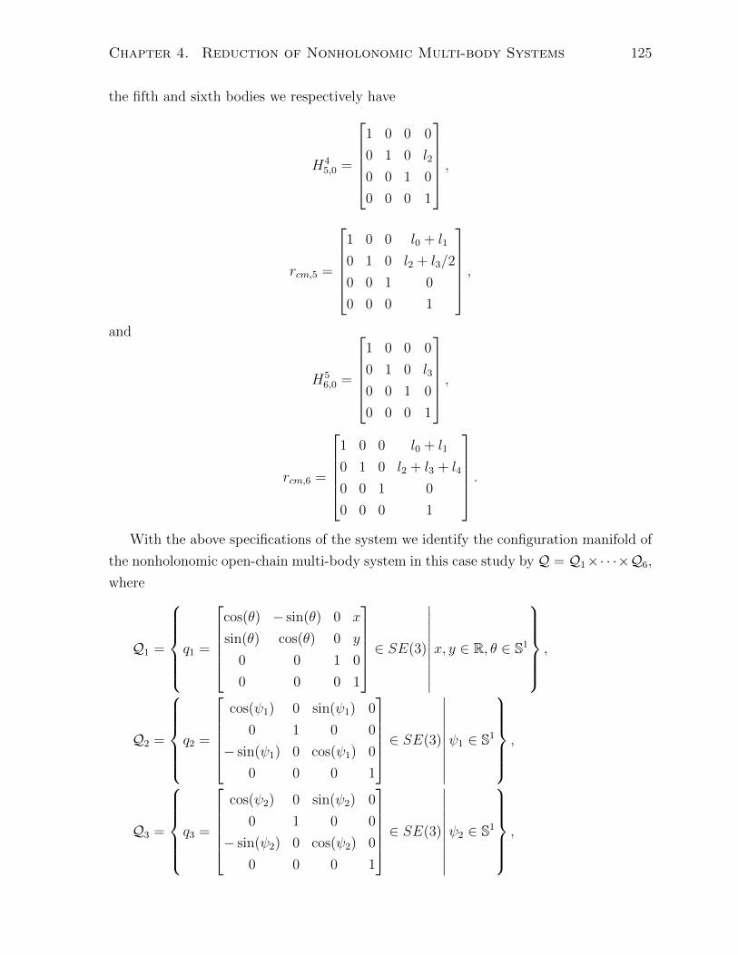
Chapter 4. Reduction of Nonholonomic Multi-body Systems 125
the fifth and sixth bodies we respectively have
H45,0 =
1 0 0 0
0 1 0 l2
0 0 1 0
0 0 0 1
,
rcm,5 =
1 0 0 l0 + l1
0 1 0 l2 + l3/2
0 0 1 0
0 0 0 1
,and
H56,0 =
1 0 0 0
0 1 0 l3
0 0 1 0
0 0 0 1
,
rcm,6 =
1 0 0 l0 + l1
0 1 0 l2 + l3 + l4
0 0 1 0
0 0 0 1
.With the above specifications of the system we identify the configuration manifold of
the nonholonomic open-chain multi-body system in this case study by Q = Q1×· · ·×Q6,
where
Q1 =
q1 =
cos(θ) − sin(θ) 0 x
sin(θ) cos(θ) 0 y
0 0 1 0
0 0 0 1
∈ SE(3)
∣∣∣∣∣∣∣∣∣∣x, y ∈ R, θ ∈ S1
,
Q2 =
q2 =
cos(ψ1) 0 sin(ψ1) 0
0 1 0 0
− sin(ψ1) 0 cos(ψ1) 0
0 0 0 1
∈ SE(3)
∣∣∣∣∣∣∣∣∣∣ψ1 ∈ S1
,
Q3 =
q3 =
cos(ψ2) 0 sin(ψ2) 0
0 1 0 0
− sin(ψ2) 0 cos(ψ2) 0
0 0 0 1
∈ SE(3)
∣∣∣∣∣∣∣∣∣∣ψ2 ∈ S1
,

Chapter 4. Reduction of Nonholonomic Multi-body Systems 126
Q4 =
q4 =
cos(ϕ1) − sin(ϕ1) 0 2(l0 + l1) sin2(ϕ1/2)
sin(ϕ1) cos(ϕ1) 0 −(l0 + l1) sin(ϕ1)
0 0 1 0
0 0 0 1
∈ SE(3)
∣∣∣∣∣∣∣∣∣∣ϕ1 ∈ S1
,
Q5 =
q5 =
1 0 0 0
0 cos(ϕ2) − sin(ϕ2) 2l2 sin2(ϕ2/2)
0 sin(ϕ2) cos(ϕ2) −l2 sin(ϕ2)
0 0 0 1
∈ SE(3)
∣∣∣∣∣∣∣∣∣∣ϕ2 ∈ S1
,
Q6 =
q6 =
1 0 0 0
0 cos(ϕ3) − sin(ϕ3) 2(l2 + l3) sin2(ϕ3/2)
0 sin(ϕ3) cos(ϕ3) −(l2 + l3) sin(ϕ3)
0 0 0 1
∈ SE(3)
∣∣∣∣∣∣∣∣∣∣ϕ3 ∈ S1
.
In order to calculate the kinetic energy for the system under study, we need to first
form the function F : Q → P =
6−times︷ ︸︸ ︷SE(3)× · · · × SE(3), which determines the pose of
the coordinate frames attached to the centres of mass of the bodies with respect to the
inertial coordinate frame.
F (q1, · · · , q6) = (q1rcm,1, q1q2rcm,2, q1q3rcm,3, q1q4rcm,4, q1q4q5rcm,5, q1q4q5q6rcm,6)
Using (3.3.31), we can calculate the kinetic energy metric for the open-chain multi-
body system. In matrix form we have the following equation for the tangent map
Tq(LF (q)−1F ) : TqQ → Lie(P)
Tq(LF (q)−1F ) =
Adr−1
cm,1· · · 0
.... . .
...
0 · · · Adr−1cm,6
id6 06×6 06×6 06×6 06×6 06×6
Adq−12
id6 06×6 06×6 06×6 06×6
Adq−13
06×6 id6 06×6 06×6 06×6
Adq−14
06×6 06×6 id6 06×6 06×6
Ad(q4q5)−1 06×6 06×6 Adq−15
id6 06×6
Ad(q4q5q6)−1 06×6 06×6 Ad(q5q6)−1 Adq−16
id6
Tq1(Lq−1
1 ι1) · · · 0
.... . .
...
0 · · · Tq6(Lq−16 ι6)
,where id6 is the 6 × 6 identity matrix, and we have the following equalities, using the

Chapter 4. Reduction of Nonholonomic Multi-body Systems 127
introduced joint parameters:
Tq1(Lq−11 ι1) =
cos(θ) − sin(θ) 0 0 0 0
sin(θ) cos(θ) 0 0 0 0
0 0 0 0 0 1
T
,
Tq2(Lq−12 ι2) =
[0 0 0 0 1 0
]T,
Tq3(Lq−13 ι3) =
[0 0 0 0 1 0
]T,
Tq4(Lq−14 ι4) =
[0 −l0 − l1 0 0 0 1
]T,
Tq5(Lq−15 ι5) =
[0 0 −l2 1 0 0
]T,
Tq6(Lq−16 ι6) =
[0 0 −l2 − l3 1 0 0
]T.
Note that, ∀H0 ∈ SE(3) that is in the following form (R0 is a rotation matrix and
p0 ∈ R3)
H0 =
[R0 p0
01×3 1
],
we calculate the AdH0 operator by
AdH0 =
[R0 p0R0
03×3 R0
].
We choose E1, · · · , E6, defined in Section 2.4, as a basis for se(3). For this case
study, the left-invariant metric h = h1⊕· · ·⊕h6 on P is identified, in the above basis, by
the following metrics on the Lie algebras of copies of SE(3) corresponding to the bodies:
(hi)e =
miid3 03×3
03×3
jx,i 0 0
0 jy,i 0
0 0 jz,i
,
where i = 1, · · · , 6, id3 and 03×3 are the 3 × 3 identity and zero matrices, respectively,
mi is the mass of Bi, and (jx,i, jy,i, jz,i) are the moments of inertia of Bi about the X,
Y and Z axes of the coordinate frame attached to the centre of mass of Bi. Note that,
we chose this coordinate frame such that its axes coincide with the principal axes of the
body Bi. For the body Bi (i = 2, · · · , 5), since we assume a symmetric cylindrical shape
whose axis is aligned with the Yi-axis, we have jx,i = jz,i. Therefore, in the coordinates

Chapter 4. Reduction of Nonholonomic Multi-body Systems 128
chosen to identify the configuration manifold (joint parameters), we have the following
matrix form for FLq
FLq = T ∗q (LF (q)−1F )
(h1)e · · · 0
.... . .
...
0 · · · (h6)e
Tq(LF (q)−1F ) =
K11(q) · · · K16(q)
.... . .
...
K61(q) · · · K66(q)
,and the kinetic energy is calculated by
Kq(q, q) =1
2qTFLq q,
where, with an abuse of notation, q is the vector corresponding to the speed of the joint
parameters.
The potential energy of the nonholonomic open-chain multi-body system is calculated
by (3.3.32). We assume a constant potential field [0 0 g]T in the inertial coordinate
frame. Therefore, using the joint parameters, we have
V (q) = g(l4m6 sin(ϕ2 + ϕ3) + l3(m5
2+m6) sin(ϕ2)).
As a result, the Hamiltonian of the nonholonomic open-chain multi-body system is cal-
culated by
H(q, p) =1
2pTFL−1
q p+ V (q),
where p is the vector of generalized momenta corresponding to the joint parameters.
The nonholonomic constraints for the multi-body system under study are the non-
slipping conditions on the wheels, i.e., B2 and B3. The linearly independent 1-forms
corresponding to the constraints are
ω11 = − sin(θ)dx+ cos(θ)dy,
ω21 = cos(θ)dx+ sin(θ)dy − cdθ − bdψ1,
ω31 = cos(θ)dx+ sin(θ)dy + cdθ − bdψ2,
where b is the radius of each wheel. The distribution D ⊂ TQ is the annihilator of these
constraint 1-forms, and it is the span of the following vector fields:∂
∂ψ1
+b
2
(cos(θ)
∂
∂x+ sin(θ)
∂
∂y− 1
c
∂
∂θ
)

Chapter 4. Reduction of Nonholonomic Multi-body Systems 129
,∂
∂ψ2
+b
2
(cos(θ)
∂
∂x+ sin(θ)
∂
∂y+
1
c
∂
∂θ
),∂
∂ϕ1
,∂
∂ϕ2
,∂
∂ϕ3
.
Here in this example, the base of the multi-body system consists of three bodies, B1,
B2 and B3, and its configuration manifold Q1 ×Q2 ×Q3 is isomorphic to G = SE(2)×SO(2)×SO(2), as a group. The kinetic and potential energy of the system are invariant
under the action of G by left translation on Q1 × Q2 × Q3. Also, the distribution D is
invariant under this action. Now, consider the action of G = SE(2) ⊂ G as a subgroup
of G, which satisfies the dimensional assumption (4.2.10) for Chaplygin systems. Using
the joint parameters, ∀(x0, y0, θ0) ∈ G we have
Φ(x0,y0,θ0)(q) = (x cos(θ0)− y sin(θ0) + x0, x sin(θ0) + y cos(θ0) + y0, θ + θ0, q1, q),
where q1 = (ψ1, ψ2) and q = (ϕ1, ϕ2, ϕ3). We have the principal G-bundle π : Q → Q =
Q2 × · · · × Q6, and using the joint parameters its corresponding principal connection
A : TQ → se(2) is defined by
Aq =
Adh︷ ︸︸ ︷cos(θ) − sin(θ) y
sin(θ) cos(θ) −x0 0 1
ThLh−1︷ ︸︸ ︷ cos(θ) sin(θ) 0
− sin(θ) cos(θ) 0
0 0 1
Aq1︷ ︸︸ ︷−b/2 −b/2
0 0
b/(2c) −b/(2c)
03×3
,
where h = (x, y, θ) is an element of Q1. And consequently, the horizontal lift map
hlq : TqQ → TqQ is
hlq =
b cos(θ)/2 b cos(θ)/2
b sin(θ)/2 b sin(θ)/2
−b/(2c) b/(2c)
03×3
id5
,where id5 is the 5× 5 identity matrix. Then, we have
FLq = hlT
q FLqhlq =
K11(q) · · · K14(q)
.... . .
...
K41(q) · · · K44(q)
,

Chapter 4. Reduction of Nonholonomic Multi-body Systems 130
where the following equalities hold:
K11(q) = ATq1K11((e1, q))Aq1 − ATq1
[K21((e1, q))
K31((e1, q))
]T−
[K21((e1, q))
K31((e1, q))
]Aq1
+
[K22((e1, q)) K23((e1, q))
K32((e1, q)) K33((e1, q))
],
K1j(q) = −ATq1K1(j+2)((e1, q)) +
[K2(j+2)((e1, q))
K3(j+2)((e1, q))
], ∀j = 2, 3, 4
Kj1(q) = K1j(q)T , ∀j = 2, 3, 4
Kij(q) = Kij((e1, q)). ∀i, j = 2, 3, 4
Here,
Aq1 =
−b/2 −b/20 0
b/(2c) −b/(2c)
.As a result, we can calculate the 2-form Ξ by (4.3.27)
Ξpq = pTFL−1q
−ATq1K11((e1, q)) +
[K21((e1, q))
K31((e1, q))
]K41((e1, q))
...
K61((e1, q))
0
b2/(2c)
0
dψ1∧dψ2 = Υ(q, p)dψ1∧dψ2,
where p is the vector of generalized momenta in the reduced space. Finally, in matrix
form we have the following reduced equations of motion for the nonholonomic multi-body
system under study:
[˙q˙p
]=
05×5 id5
−id5
0 Υ(q, p) 0 0 0
−Υ(q, p) 0 0 0 0
0 0 0 0 0
0 0 0 0 0
0 0 0 0 0
∂H∂q∂H∂p
,
where H is calculated by (4.3.26), with V (q) = V ((e1, q)).
Example 4.6.2. In this example, we study the two-step reduction of the dynamical
equations of a two-d.o.f. crane on a four-wheel car whose top and side view in the

Chapter 4. Reduction of Nonholonomic Multi-body Systems 131
Figure 4.3: An example of a crane
initial configuration is shown in Figure 4.3. Using the indexing introduced in the pre-
vious section and starting with the car without the rear wheels and the crane as B1,
we first number the bodies and joints. The following graph shows the structure of the
nonholonomic open-chain multi-body system.
B4 B2J5J4
B5
B0J1
B1
J2
J3B3
J6B6
Similar to the previous example, we then identify the relative configuration manifolds
corresponding to the joints of the robotic system. We identify the elements of the relative
configuration manifold corresponding to the first joint, which is a three-d.o.f. planar joint,
by
Q01 =
H21 =
cos(θ) − sin(θ) 0 x
sin(θ) cos(θ) 0 y
0 0 1 0
0 0 0 1
∈ SE(3)
∣∣∣∣∣∣∣∣∣∣x, y ∈ R, θ ∈ S1
.
Here, (x, y) is the position of C with respect to the inertial coordinate frame and θ is the
angle between the X1-axis and X0-axis (see Figure 4.4). The second joint is a one-d.o.f.
revolute joint between B2 and B1, and its corresponding relative configuration manifold

Chapter 4. Reduction of Nonholonomic Multi-body Systems 132
Figure 4.4: The coordinate frames attached to the bodies of the crane
is given by
Q12 =
H12 =
cos(ψ1) − sin(ψ1) 0 l
sin(ψ1) cos(ψ1) 0 0
0 0 1 0
0 0 0 1
∈ SE(3)
∣∣∣∣∣∣∣∣∣∣ψ1 ∈ S1
,
where l is the distance between the front and rear wheels. Similarly, for the third joint
we have
Q13 =
H13 =
cos(ϕ1) − sin(ϕ1) 0 l1
sin(ϕ1) cos(ϕ1) 0 0
0 0 1 0
0 0 0 1
∈ SE(3)
∣∣∣∣∣∣∣∣∣∣ϕ1 ∈ S1
.
The forth and fifth joints are one-d.o.f. revolute joints whose axes of revolution are the
Yi-axis (i = 4, 5). The relative configuration manifolds of these joints are identified by
Q24 =
H24 =
cos(ψ2) 0 sin(ψ2) 0
0 1 0 c
− sin(ψ2) 0 cos(ψ2) 0
0 0 0 1
∈ SE(3)
∣∣∣∣∣∣∣∣∣∣ψ2 ∈ S1
,

Chapter 4. Reduction of Nonholonomic Multi-body Systems 133
Q25 =
H25 =
cos(ψ3) 0 sin(ψ3) 0
0 1 0 −c− sin(ψ3) 0 cos(ψ3) 0
0 0 0 1
∈ SE(3)
∣∣∣∣∣∣∣∣∣∣ψ3 ∈ S1
,
where c is the distance between the steering point and the front wheels. Note that, if
we assume that the front wheels are rotating together, then we can substitute the front
wheels with a cylinder. Finally, the sixth joint is a one-d.o.f. revolute joint with the
Y6-axis being its axis of revolution. So, we have
Q56 =
H56 =
cos(ϕ2) 0 sin(ϕ2) 0
0 1 0 0
− sin(ϕ2) 0 cos(ϕ2) l2
0 0 0 1
∈ SE(3)
∣∣∣∣∣∣∣∣∣∣ϕ2 ∈ S1
.
We assume that the initial pose of B1 with respect to the inertial coordinate frame
H01,0 is the identity element of SE(3). As a result, the initial pose of the centre of mass
of B1 with respect to B0 is
rcm,1 =
1 0 0 l0
0 1 0 0
0 0 1 0
0 0 0 1
.For the second and third body, the initial relative pose with respect to B1 is
H12,0 =
1 0 0 l
0 1 0 0
0 0 1 0
0 0 0 1
,
H13,0 =
1 0 0 l1
0 1 0 0
0 0 1 0
0 0 0 1
,and we have
rcm,2 =
1 0 0 l
0 1 0 0
0 0 1 0
0 0 0 1
,

Chapter 4. Reduction of Nonholonomic Multi-body Systems 134
rcm,3 =
1 0 0 l1
0 1 0 l2/2
0 0 1 0
0 0 0 1
,where we assume that the centre of mass of B3 is located in the middle of the body. The
initial relative pose of B4 and B5 with respect to B2 is
H2i,0 =
1 0 0 0
0 1 0 ±c0 0 1 0
0 0 0 1
,
and the relative pose of the centre of mass of B4 and B5 with respect to the inertial
coordinate frame is
rcm,i =
1 0 0 l
0 1 0 ±c0 0 1 0
0 0 0 1
,where i = 4, 5 and plus and minus signs refer to B4 and B5, respectively. For the sixth
body we have
H36,0 =
1 0 0 0
0 1 0 l2
0 0 1 0
0 0 0 1
,
rcm,6 =
1 0 0 l1
0 1 0 0
0 0 1 l2
0 0 0 1
,where we assume that the centre of mass of this body is at the sixth joint J6.
Knowing the above specifications of the system, we identify the configuration manifold
of the nonholonomic open-chain multi-body system in this case study by Q = Q1×· · ·×

Chapter 4. Reduction of Nonholonomic Multi-body Systems 135
Q6, where
Q1 =
q1 =
cos(θ) − sin(θ) 0 x
sin(θ) cos(θ) 0 y
0 0 1 0
0 0 0 1
∈ SE(3)
∣∣∣∣∣∣∣∣∣∣x, y ∈ R, θ ∈ S1
,
Q2 =
q2 =
cos(ψ1) − sin(ψ1) 0 2l sin2(ψ1/2)
sin(ψ1) cos(ψ1) 0 −l sin(ψ1)
0 0 1 0
0 0 0 1
∈ SE(3)
∣∣∣∣∣∣∣∣∣∣ψ1 ∈ S1
,
Q3 =
q3 =
cos(ϕ1) − sin(ϕ1) 0 2l1 sin2(ϕ1/2)
sin(ϕ1) cos(ϕ1) 0 −l1 sin(ϕ1)
0 0 1 0
0 0 0 1
∈ SE(3)
∣∣∣∣∣∣∣∣∣∣ϕ1 ∈ S1
,
Q4 =
q4 =
cos(ψ2) 0 sin(ψ2) 2l sin2(ψ2/2)
0 1 0 0
− sin(ψ2) 0 cos(ψ2) l sin(ψ2)
0 0 0 1
∈ SE(3)
∣∣∣∣∣∣∣∣∣∣ψ2 ∈ S1
,
Q5 =
q5 =
cos(ψ3) 0 sin(ψ3) 2l sin2(ψ3/2)
0 1 0 0
− sin(ψ3) 0 cos(ψ3) l sin(ψ3)
0 0 0 1
∈ SE(3)
∣∣∣∣∣∣∣∣∣∣ψ3 ∈ S1
,
Q6 =
q6 =
cos(ϕ2) 0 sin(ϕ2) 2l1 sin2(ϕ2/2)− l2 sin(ϕ2)
0 1 0 0
− sin(ϕ2) 0 cos(ϕ2) l1 sin(ϕ2) + 2l2 sin2(ϕ2/2)
0 0 0 1
∈ SE(3)
∣∣∣∣∣∣∣∣∣∣ϕ2 ∈ S1
.
In order to calculate the kinetic energy for the system under study, we need to first
form the function F : Q → P =
6−times︷ ︸︸ ︷SE(3)× · · · × SE(3), which determines the pose of
the coordinate frames attached to the centres of mass of the bodies with respect to the
inertial coordinate frame.
F (q1, · · · , q5) = (q1rcm,1, q1q2rcm,2, q1q3rcm,3, q1q2q4rcm,4, q1q2q5rcm,5, q1q3q6rcm,6)
Using (3.3.31), we can calculate the kinetic energy metric for the open-chain multi-

Chapter 4. Reduction of Nonholonomic Multi-body Systems 136
body system. In matrix form we have the following equation for the tangent map
Tq(LF (q)−1F ) : TqQ → Lie(P)
Tq(LF (q)−1F ) =
Adr−1
cm,1· · · 0
.... . .
...
0 · · · Adr−1cm,6
id6 06×6 06×6 06×6 06×6 06×6
Adq−12
id6 06×6 06×6 06×6 06×6
Adq−13
06×6 id6 06×6 06×6 06×6
Ad(q2q4)−1 Adq−14
06×6 id6 06×6 06×6
Ad(q2q5)−1 Adq−15
06×6 06×6 id6 06×6
Ad(q3q6)−1 06×6 Adq−16
06×6 06×6 id6
Tq1(Lq−1
1 ι1) · · · 0
.... . .
...
0 · · · Tq6(Lq−16 ι6)
.where we have the following equalities, using the introduced joint parameters:
Tq1(Lq−11 ι1) =
cos(θ) − sin(θ) 0 0 0 0
sin(θ) cos(θ) 0 0 0 0
0 0 0 0 0 1
T
,
Tq2(Lq−12 ι2) =
[0 −l 0 0 0 1
]T,
Tq3(Lq−13 ι3) =
[0 −l1 0 0 0 1
]T,
Tq4(Lq−14 ι4) =
[0 0 l 0 1 0
]T,
Tq5(Lq−15 ι5) =
[0 0 l 0 1 0
]T,
Tq6(Lq−16 ι6) =
[−l2 0 l1 0 1 0
]T.
We choose E1, · · · , E6 as a basis for se(3) and define the following metrics on the
Lie algebras of copies of SE(3) corresponding to bodies:
(hi)e =
miid3 03×3
03×3
jx,i 0 0
0 jy,i 0
0 0 jz,i
,
where i = 1, · · · , 6, mi is the mass of Bi, and (jx,i, jy,i, jz,i) are the moments of inertia of
Bi about the Xi, Yi and Zi axes of the coordinate frame attached to the centre of mass

Chapter 4. Reduction of Nonholonomic Multi-body Systems 137
of Bi. Note that, we chose this coordinate frame such that its axes coincide with the
principal axes of the body Bi. For the body Bi (i = 2, · · · , 6), we assume a symmetric
cylindrical shape. The cylinder axis is aligned with the Yi-axis for i = 2, 4, 5, so we have
jx,i = jz,i. Similarly, for the bodies B3 and B6, the cylinder axes are aligned with Z3 and
X6 axes, and we have the equalities jx,3 = jy,3 and jy,6 = jz,6. Also, since the wheels
are assumed identical, only the dynamic parameters of B4 is going to appear in the
calculations. Therefore, in the coordinates chosen to identify the configuration manifold
(joint parameters), we have the following matrix form for FLq
FLq = T ∗q (LF (q)−1F )
(h1)e · · · 0
.... . .
...
0 · · · (h6)e
Tq(LF (q)−1F ) =
K11(q) · · · K16(q)
.... . .
...
K61(q) · · · K66(q)
.Here, we have
K11(q) =
mtot 0 − sin(θ)(lm2 + 2lm4 + l0m1 + l1m3 + l1m6)
? mtot cos(θ)(lm2 + 2lm4 + l0m1 + l1m3 + l1m6)
? ? jz,tot
K21(q) = K12(q)T =
[0 0 2m4c
2 + jx,2 + 2Jx,4
],
K31(q) = K13(q)T =[0 0 jz,3 + jx,6 sin2(ϕ2) + jy,6 cos2(ϕ2)
],
Ki1(q) = K1i(q)T =
[0 0 0
],∀i = 4, 5, 6
K22(q) = 2m4c2 + jx,2 + 2jx,4, Ki2 = K2i = 0, ∀i = 3, · · · , 6
K33(q) = jz,3 + jx,6 sin2(ϕ2) + jy,6 cos2(ϕ2), Ki3 = K3i = 0,∀i = 4, 5, 6
K44(q) = jy,4, Ki4 = K4i = 0,∀i = 5, 6
K55(q) = jy,4, K65 = K56 = 0, K66(q) = jy,6,
where
mtot = m1 +m2 +m3 + 2m4 +m6,
jz,tot = jz,1 + jx,2 + jz,3 + 2jx,4 + jx,6 + l2m2 + 2l2m4 + l20m1 + l21m3
+ l21m6 + 2c2m4 − jx,6 cos2(ϕ2) + jy,6 cos2(ϕ2).
For K11(q), we did not include the lower diagonal elements, since the matrix is symmetric.

Chapter 4. Reduction of Nonholonomic Multi-body Systems 138
The kinetic energy is calculated by
Kq(q, q) =1
2qTFLq q,
where, with an abuse of notation, q is the vector corresponding to the speed of the joint
parameters.
For this case study, the potential energy of the nonholonomic open-chain multi-body
system is constant, and it does not enter the dynamical equation. As a result, the
Hamiltonian of the nonholonomic open-chain multi-body system is calculated by
H(q, p) =1
2pTFL−1
q p,
where p is the vector of generalized momenta corresponding to the joint parameters.
The nonholonomic constraints for the multi-body system under study are the non-
slipping conditions on the wheels, i.e., B4 and B5. The linearly independent 1-forms
corresponding to the constraints are
ω11 = − sin(θ)dx+ cos(θ)dy,
ω21 = − sin(θ + ψ1)dx+ cos(θ + ψ1)dy + l cos(ψ1)dθ,
ω31 = cos(θ + ψ1)dx+ sin(θ + ψ1)dy + (l sin(ψ1)− c)dθ − cdψ1 − bdψ2,
ω41 = cos(θ + ψ1)dx+ sin(θ + ψ1)dy + (l sin(ψ1) + c)dθ + cdψ1 − bdψ3,
where b is the radius of each wheel. The distribution D ⊂ TQ is the annihilator of these
constraint 1-forms, and it is the span of the following vector fields:∂
∂ψ1
+cl cos(ψ1)
l − c sin(ψ1)
(cos(θ)
∂
∂x+ sin(θ)
∂
∂y+
tan(ψ1)
l
∂
∂θ+
2
b cos(ψ1)
∂
∂ψ3
),∂
∂ψ2
+bl cos(ψ1)
l − c sin(ψ1)
(cos(θ)
∂
∂x+ sin(θ)
∂
∂y+
tan(ψ1)
l
∂
∂θ+l + c sin(ψ1)
bl cos(ψ1)
∂
∂ψ3
),∂
∂ϕ1
,∂
∂ϕ2
.
Here in this example, the base of the multi-body system consists of four bodies, B1, B2,
B4 and B5, and its configuration manifold is Q1×Q2×Q4×Q5. The Hamiltonian of the
system H and the distribution D are invariant under the action of G = Q1×Q3×Q4×Q5,
which is isomorphic to SE(2)× SO(2)× SO(2)× SO(2) as a group, by left translation.
Now, consider the action of G = Q1 × Q5 ⊂ G as a subgroup of G, which satisfies
the dimensional assumption (4.2.10) for Chaplygin systems. Using the joint parameters,
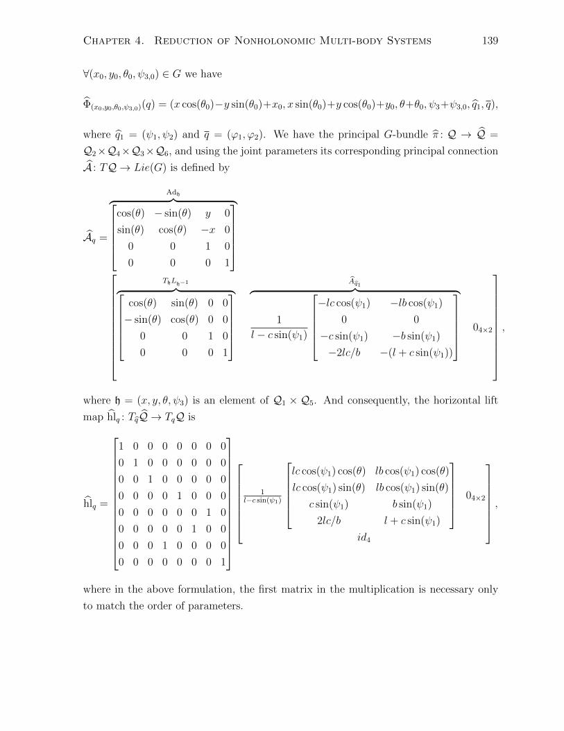
Chapter 4. Reduction of Nonholonomic Multi-body Systems 139
∀(x0, y0, θ0, ψ3,0) ∈ G we have
Φ(x0,y0,θ0,ψ3,0)(q) = (x cos(θ0)−y sin(θ0)+x0, x sin(θ0)+y cos(θ0)+y0, θ+θ0, ψ3+ψ3,0, q1, q),
where q1 = (ψ1, ψ2) and q = (ϕ1, ϕ2). We have the principal G-bundle π : Q → Q =
Q2×Q4×Q3×Q6, and using the joint parameters its corresponding principal connection
A : TQ → Lie(G) is defined by
Aq =
Adh︷ ︸︸ ︷cos(θ) − sin(θ) y 0
sin(θ) cos(θ) −x 0
0 0 1 0
0 0 0 1
ThLh−1︷ ︸︸ ︷cos(θ) sin(θ) 0 0
− sin(θ) cos(θ) 0 0
0 0 1 0
0 0 0 1
Aq1︷ ︸︸ ︷1
l − c sin(ψ1)
−lc cos(ψ1) −lb cos(ψ1)
0 0
−c sin(ψ1) −b sin(ψ1)
−2lc/b −(l + c sin(ψ1))
04×2
,
where h = (x, y, θ, ψ3) is an element of Q1 × Q5. And consequently, the horizontal lift
map hlq : TqQ → TqQ is
hlq =
1 0 0 0 0 0 0 0
0 1 0 0 0 0 0 0
0 0 1 0 0 0 0 0
0 0 0 0 1 0 0 0
0 0 0 0 0 0 1 0
0 0 0 0 0 1 0 0
0 0 0 1 0 0 0 0
0 0 0 0 0 0 0 1
1
l−c sin(ψ1)
lc cos(ψ1) cos(θ) lb cos(ψ1) cos(θ)
lc cos(ψ1) sin(θ) lb cos(ψ1) sin(θ)
c sin(ψ1) b sin(ψ1)
2lc/b l + c sin(ψ1)
04×2
id4
,
where in the above formulation, the first matrix in the multiplication is necessary only
to match the order of parameters.

Chapter 4. Reduction of Nonholonomic Multi-body Systems 140
Then, we have
FLq = hlT
q FLqhlq =
K11(q) · · · K14(q)
.... . .
...
K41(q) · · · K44(q)
,where the following equalities hold:
K11(q) = ATq1
[K11((e1, q)) K15((e1, q))
K51((e1, q)) K55((e1, q))
]Aq1 − ATq1
[K21((e1, q)) K25((e1, q))
K41((e1, q)) K45((e1, q))
]T
−
[K21((e1, q)) K25((e1, q))
K41((e1, q)) K45((e1, q))
]Aq1 +
[K22((e1, q)) K24((e1, q))
K42((e1, q)) K44((e1, q))
],
K12(q) = −ATq1
[K13((e1, q))
K53((e1, q))
]+
[K23((e1, q))
K43((e1, q))
]= K21(q)T ,
K13(q) = −ATq1
[K16((e1, q))
K56((e1, q))
]+
[K26((e1, q))
K46((e1, q))
]= K31(q)T ,[
K22(q) K23(q)
K32(q) K33(q)
]=
[K33((e1, q)) K36((e1, q))
K63((e1, q)) K66((e1, q))
].
Here,
Aq1 =1
l − c sin(ψ1)
−lc cos(ψ1) −lb cos(ψ1)
0 0
−c sin(ψ1) −b sin(ψ1)
−2lc/b −(l + c sin(ψ1))
.As a result, we can calculate the 2-form Ξ by (4.3.27)
Ξpq = pTFL−1q
−ATq1
[K11((e1, q)) K15((e1, q))
K51((e1, q)) K55((e1, q))
]+
[K21((e1, q)) K25((e1, q))
K41((e1, q)) K45((e1, q))
][K31((e1, q)) K35((e1, q))
K61((e1, q)) K65((e1, q))
]
−b(c− l sin(ψ1))
0
−b cos(ψ1)
−2c cos(ψ1)
l
(l − c sin(ψ1))2dψ1 ∧ dψ2 = Υ(q, p)dψ1 ∧ dψ2,
where p is the vector of generalized momenta in the reduced space. Finally, in matrix

Chapter 4. Reduction of Nonholonomic Multi-body Systems 141
form we have the following reduced equations of motion for the nonholonomic multi-body
system under study:
[˙q˙p
]=
04×4 id4
−id4
0 Υ(q, p) 0 0
−Υ(q, p) 0 0 0
0 0 0 0
0 0 0 0
∂H∂q∂H∂p
,
where H is calculated by (4.3.26), with V (q) = 0.
4.6.1 Further Reduction of the System
In this subsection we investigate if the system under study demonstrates any conserved
quantity due to the action of a bigger symmetry group (bigger than Q1 × Q5). In this
case study, since originally FLq is independent of ϕ1, the Hamiltonian H is invariant
under the cotangent lift of the action of N = Q3 by left translation. Using the joint
parameters, for any ϕ1,0 we have the action of N on T ∗Q defined as
T ∗Φϕ1,0(ψ1, ψ2, ϕ1, ϕ2, pψ1 , pψ2 , pϕ1 , pϕ2) = (ψ1, ψ2, ϕ1 + ϕ1,0, ϕ2, pψ1 , pψ2 , pϕ1 , pϕ2),
where (ψ1, ψ2, ϕ1, ϕ2, pψ1 , pψ2 , pϕ1 , pϕ2) is a coordinate for T ∗Q, which can be considered
as the reduced space of joint parameters and their corresponding momenta. Also, it is
easy to check that ∀ζ ∈ Lie(N ),
ιζT∗Q
Ξ = 0,
where based on the definition of the cotangent lifted action of N , defined above, we have
φq =[0 0 1 0
]T,
ζT ∗Q =
[φq(ζ)
04×1
]=[0 0 ζ 0 0 0 0 0
]T.
As a result, we have that the momentum map Mq : T ∗q Q → Lie∗(N ) for the N -action and
corresponding to the 2-form Ωcan is conserved along the solution curves of the reduced
system. Here, the momentum map is defined by
Mq =[0 0 1 0
].

Chapter 4. Reduction of Nonholonomic Multi-body Systems 142
We have a principal bundle π : Q → Q = Q2 ×Q4 ×Q6 with the (mechanical) principal
connection Aq : TqQ → Lie(N )
Aq =1
l − c sin(ψ1)
[c sin(ψ1) b sin(ψ1) l − c sin(ψ1) 0
].
For a regular value of the momentum map ϑ ∈ Lie∗(N ), the coadjoint isotropy group
Nϑ = N , and the level set of the momentum map is
M−1
(ϑ) =
(ψ1, ψ2, ϕ1, ϕ2, pψ1 , pψ2 , pϕ1 , pϕ2) ∈ T ∗Q∣∣∣ pϕ1 = ϑ
⊂ T ∗Q.
Also, we have
αϑ =ϑ
l − c sin(ψ1)(c sin(ψ1)dψ1 + b sin(ψ1)dψ2 + (l − c sin(ψ1))dϕ1) ∈ Ω1(Q),
and hence,
Ξϑ =ϑbl cos(ψ1)
(l − c sin(ψ1))2dψ1 ∧ dψ2 ∈ Ω2(T ∗Q).
We then can calculate the map ϕ−1ϑ : T ∗Q → M
−1(ϑ)/N by
ϕ−1ϑ (ψ1, ψ2, ϕ2, pψ1 , pψ2 , pϕ2) = (ψ1, ψ2, ϕ2, pψ1 +
ϑc sin(ψ1)
l − c sin(ψ1), pψ2 +
ϑb sin(ψ1)
l − c sin(ψ1), pϕ2).
As a result, we determine the 2-forms Ξϑ ∈ Ω2(T ∗Q):
Ξϑ = Υ(q, p)dψ1 ∧ dψ2,
where
Υ(q, p) := Υ(ψ1, ψ2, 0, ϕ2, pψ1 +ϑc sin(ψ1)
l − c sin(ψ1), pψ2 +
ϑb sin(ψ1)
l − c sin(ψ1), ϑ, pϕ2).
Finally, we have the reduced equations of motion in T ∗Q as:
[˙q˙p
]=
03×3 id3
−id3
0 Υ(q, p) + ϑbl cos(ψ1)
(l−c sin(ψ1))2 0
−Υ(q, p)− ϑbl cos(ψ1)(l−c sin(ψ1))2 0 0
0 0 0
∂Hϑ∂q∂Hϑ∂p
,

Chapter 4. Reduction of Nonholonomic Multi-body Systems 143
where
Hϑ(q, p) = H(ψ1, ψ2, 0, ϕ2, pψ1 +ϑc sin(ψ1)
l − c sin(ψ1), pψ2 +
ϑb sin(ψ1)
l − c sin(ψ1), ϑ, pϕ2).
Chapter 5
Concurrent Control of Free-base,
Open-chain Multi-body Systems
This chapter presents a unified geometric approach to output tracking control of under-
actuated holonomic and nonholonomic open-chain multi-body systems with multi-d.o.f.
joints, and constant (non necessarily zero) momentum. We focus our attention on the
case of holonomic and nonholonomic open-chain multi-body systems with symmetry,
whose joints corresponding to the symmetry group are unactuated. The immediate ap-
plications of this case are free-base space manipulators with non-zero total momentum
and mobile manipulators. We first formalize the control problem, and rigorously state
an output tracking problem for such systems in Problem 5.1.10 in Section 5.1.2. Then,
in Section 5.2 we introduce a geometrical definition of the end-effector pose and velocity
error. The main contribution of this chapter is brought in Section 5.3, where we solve for
the input-output linearization of the highly nonlinear problem of coupled manipulator
and base dynamics with non-zero momentum subject to holonomic and nonholonomic
constraints. This enables us to design a coordinate-independent linear controller, such
as a proportional-derivative with feed-forward, for concurrently controlling a free-base,
open-chain multi-body system with non-zero momentum and under holonomic and/or
nonholonomic constraints, which is discussed in Section 5.4. Finally, by defining a Lya-
punov function we prove in Theorem 5.4.2 that the closed-loop system is exponentially
stable. A detailed case study in Section 5.5 concludes this chapter.
5.1 Problem Statement
In this section we formally state an output trajectory tracking control problem for free-
base, open-chain multi-body systems with multi-d.o.f. holonomic (non-zero momentum)
144

Chapter 5. Concurrent Control of Multi-body Systems 145
and nonholonomic joints. The output of such systems is usually the pose of the extremi-
ties and the base. More generally, one may be interested in controlling only parts of the
motion of the extremities and the base. For example, in the case of a free-floating space
manipulator, one may want to control the position of the end-effector and the orientation
of the base. In this case, the output manifold of the open-chain multi-body system is a
quotient manifold, which is locally identified by a submanifold of the space of all possible
poses of the end-effector and the base. In this chapter, by output manifold we mean a
submanifold of the smooth manifold that consists of all possible poses of the extremities
and the base of a free-base, open-chain multi-body system.
5.1.1 Mathematical Formalization and Assumptions
Let a holonomic or nonholonomic open-chain multi-body system with symmetry be de-
noted by (T ∗Q,Ωcan, H,K,G) or (T ∗Q,Ωcan,D, H,K,G), where in the holonomic case
G = Q1 and G = G × N for a nonholonomic system. Also, we denote the number of
independent control directions by nc; it is equal to dim(Q)− dim(G).
CON1) We assume that the multi-body system is invariant under the action of G, in the
sense introduced in Chapter 3 and 4.
This assumption implies that in the holonomic case the open-chain multi-body system
has a conserved momentum. Note that in this case the constant momentum does not
have to be zero. As for the nonholonomic open-chain multi-body system, we assume that
it is a Chaplygin system, and it possibly has a conserved quantity. We recall that control
directions are modelled by 1-forms on Q.
CON2) We also assume that there is no control input collocated with the G orbits for a
holonomic or nonholonomic multi-body system with symmetry. That is, for a set of
linearly independent differential 1-forms Ti ∈ Ω1(Q)| i = 1, · · · , nc corresponding
to the directions of the (available) control inputs (in the form of control force or
torque), ∀ξ ∈ Lie(G) we have
ιξQTi = 0. i = 1, · · · , nc (5.1.1)
This condition guarantees that there is no actuator at the first joint for a holonomic
open-chain multi-body system, and also the actuators of a nonholonomic open-chain
multi-body system do not overlap with the directions of the nonholonomic constraints.

Chapter 5. Concurrent Control of Multi-body Systems 146
Definition 5.1.1. A holonomic or nonholonomic open-chain multi-body system with
symmetry is called free-base, if we have the assumption CON2, i.e., the joints corre-
sponding to the symmetry group G are unactuated.
Corollary 5.1.2. Let the codistribution F := spanC∞(Q) Ti ∈ Ω1(Q)| i =
1, · · · , nc annihilate the distribution spanC∞(Q) ξQ ∈ X(Q)| ξ ∈ Lie(G). This distri-
bution is involutive and it specifies a global foliation of Q whose leaves are the orbits G(embedded submanifolds of Q), since the G-action is free and proper. Based on Frobenius
theorem [43], for any point there exists an open neighbourhood U ⊂ Q there exist nc exact
1-forms Ui|U = dhi (i = 1, · · · , nc), where hi ∈ C∞(U), such that we have
F|U = spanC∞(U)
Ui ∈ Ω1(U)
∣∣Ui = dhi, i = 1, · · · , nc. (5.1.2)
We say that the codistribution F is integrable, if its corresponding distribution on TQ is
integrable.
Proposition 5.1.3. The 1-forms Ui ∈ Ω1(U) for all i = 1, · · · , nc are locally G invariant.
Proof. This result follows immediately from
LξQUi = d(ιξQUi) + ιξQdUi = ιξQddhi = 0, i = 1, · · · , nc
since based on the previous corollary we have Ui|U = dhi.
CON3) From now on, we assume that (globally) there exist nc closed 1-forms Ui’s whose
span is the codistribution F , and we use them as a basis for F . As a result, the
Ui’s are basic 1-forms with respect to the G action.
In a case of free-base manipulator, CON3 means that there exist sufficient number of
control directions that are independent of the full (holonomic) or partial (nonholonomic)
pose of the base. We specify a set of n2c smooth functions yij ∈ C∞(Q)| i, j = 1, · · · , nc
by Ui =∑nc
j=1 yijTj.
Definition 5.1.4. Under the assumption CON3, for a free-base holonomic or nonholo-
nomic open-chain multi-body system with symmetry, we call (T ∗Q,Ωcan, H,K,G, Uinci=1)
or (T ∗Q,Ωcan, H,K,D,G, Uinci=1), respectively, a controlled multi-body system with sym-
metry.
Let ui ∈ C2(T ∗Q× R)| i = 1, · · · , nc be a set of twice differentiable functions on
the extended phase space (by the time direction). We define the control input for a

Chapter 5. Concurrent Control of Multi-body Systems 147
controlled multi-body system with symmetry by
nc∑i=1
uiUi. (5.1.3)
We write the control Hamilton’s equation for a controlled multi-body system with
symmetry as
ιXCΩcan = dH −f∑s=1
κsT∗πQ(ωs) +
nc∑i=1
uiT∗πQ(Ui), (5.1.4)
ωs(TπQ(XC)) = 0 s = 1, · · · , f
where T ∗πQ : T ∗Q → T ∗(T ∗Q) is the induced map on the cotangent bundles by the
canonical projection map of the cotangent bundle πQ : T ∗Q → Q. Here, ωs’s are the
constraint 1-forms defining the nonholonomic distribution D and κs’s are the Lagrange
multipliers.
Remark 5.1.5. Note that this equation is a generic Hamilton’s equation, which applies
to both holonomic and nonholonomic multi-body systems, and in the holonomic case
ωs ≡ 0.
Remark 5.1.6. Also, note that the vector field XC in this equation is a time-dependent
vector field on T ∗Q, since the ui’s are functions of time.
We are interested in controlling the motion of the extremities (the base of the multi-
body system is also considered as one of the extremities) of a multi-body system with
symmetry, in certain directions. Let ne be the number of extremities of a controlled multi-
body system with symmetry, and let FKi : Q1 × · · · × Qi0 → SE(3) (for i = 1, · · · , ne)be the forward kinematics maps for the extremities, defined by
FKi(q1, · · · , qi0) = q1 · · · qi0r0i0,0, i = 1, · · · , ne (5.1.5)
where Bi0 is the ith extremity (base body is considered as the first extremity, i.e., 10 = 1),
r0i0,0∈ P0
∼= SE(3) is the initial pose of the ith extremity with respect to the inertial
coordinate frame. Note that only the elements of the relative configuration manifolds
of the joints that are in the path of bodies connecting B0 to Bi0 are involved in the
above equation (see Section 3.3.1). For the ith extremity, we identify it by the embedded
submanifold Ri ⊆ SE(3), which corresponds the directions of motion of Bi0 that we
are interested in. By FK : Q → R := R1 × · · · × Rne we denote the collection of

Chapter 5. Concurrent Control of Multi-body Systems 148
FKi composed with the projection maps ri : SE(3) → Ri, such that we have ri ιRi =
idRi . Here, ιRi : Ri → SE(3) is the canonical inclusion map, and idRi indicates the
identity map on Ri. We also denote the induced projection map that projects Pe :=ne−times︷ ︸︸ ︷
SE(3)× · · · × SE(3) to R by r : Pe → R. The manifold R is called the output manifold,
and no := dim(R) indicates the dimension of the output.
Note that in general the projection map r is not defined globally. In the cases where
this projection does not make sense globally, we define it in a tubular neighbourhood in
Pe around the submanifold R. When we are working in an appropriate local coordinates
for Pe, the projection map r can be considered as a projection to an affine subspace of
the Euclidean space.
Consider a curve in the output manifold γ : R → R corresponding to the desired
motion of the extremities of a controlled multi-body system with symmetry.
CON4) It is always assumed that the curve t 7→ γ(t) is a feasible trajectory for a controlled
holonomic or nonholonomic open-chain multi-body system. That is, it respects the
nonholonomic constraints and the momentum conservation, and also it is in the
image of the forward kinematics map FK with a full rank Jacobian.
CON5) We also assume that the number of control inputs nc is greater than or equal to
the dimension of the output manifold, i.e., D = dim(Q) ≥ nc ≥ no.
Remark 5.1.7. Condition CON5 together with the fact that the control directions are
linearly independent guarantee local controllability of a controlled holonomic or nonholo-
nomic open-chain multi-body system with symmetry at the configurations away from the
singularities of the Jacobian introduced in Section 5.3 [72]. As a result, in the following
we assume that a controlled holonomic or nonholonomic open-chain multi-body system
with symmetry is always away from singular configurations.
Problem 5.1.8 (Control Problem). Let (T ∗Q,Ωcan, H,K,D,G, Uinci=1) be a controlled
multi-body system with symmetry, and let γ : R→ R be a desired motion of its extremi-
ties. Find a set of twice differentiable functions ui ∈ C2(T ∗Q× R)| i = 1, · · · , nc, such
that the output FK(q(t)) tracks the curve γ with an exponentially decreasing error. We
can formulate the controlled system as
Controlled System: ιXCΩcan = dH −f∑s=1
κsT∗πQ(ωs) +
nc∑i=1
ui
nc∑j=1
yijT∗πQ(Tj),
Nonholonomic Constraints: ωs(TπQ(XC)) = 0, s = 1, · · · , f (5.1.6)
Output: FK(q(t)) = (r1(q1(t)), r2(q1(t) · · · q20(t)), · · · , rne(q1(t) · · · qne0(t))).

Chapter 5. Concurrent Control of Multi-body Systems 149
Note that we defined the problem for a nonholonomic open-chain multi-body system with
symmetry. For the holonomic case, we have no constraint 1-form ωs in (5.1.6).
This problem is not precise yet, since we have not defined the error, nor the expo-
nential stability on manifolds. After reformulating the problem in the following section,
we rigorously define the error in Section 5.2 and the exponential stability in Definition
5.4.1.
5.1.2 Reduced Hamilton’s Equation and Reconstruction
In this section, we use the reduction theories developed in the previous chapters and
their corresponding reconstruction equations to reformulate Problem 5.1.8, in the re-
duced phase space. One of the premises of this section is to introduce a notation to treat
holonomic and nonholonomic cases at the same time. We denote a reduced holonomic
(nonholonomic) open-chain multi-body system by (S ⊆ T ∗Q, Ω, H, K), where S is the
reduced phase space, which is a vector sub-bundle of T ∗Q, Ω ∈ Ω2(S) is the (almost)
symplectic 2-form on the reduced phase space, H : S → R is the reduced Hamiltonian,
and ∀q ∈ Q we have the induced metric Kq : TqQ × TqQ → R on the reduced config-
uration manifold Q. The reduced Hamilton’s equation for the reduced holonomic or
nonholonomic multi-body system (S, Ω, H, K) reads
ιXΩ = dH, (5.1.7)
where for the holonomic case this equation is equivalent to (3.2.26) or (3.3.44), and
for the nonholonomic case it is (4.2.19) or (4.5.38). In order to control the extremities
of a controlled multi-body with symmetry in the inertial coordinate frame, not only
we need the reduced Hamilton’s equation but also the equations corresponding to the
reduced parameters of the system. The process of recovering these equations is called
reconstruction.
For a holonomic open-chain multi-body system with symmetry, where G = Q1, the
reconstruction yields the velocity of B1 (base) with respect to the inertial coordinate
frame and expressed in the coordinate frame attached to B1 (body velocity):
Tq1Lq−11
(q1) = K−1
11 (q)Ad∗χµ(q1)(µ)− Aq q, (5.1.8)
where µ ∈ Lie∗(G) is the constant momentum of the system, K11(q) is defined in Lemma
3.3.4, χµ : Uµ → Q1 is the embedding map corresponding to the local trivialization of
the principal bundle Q1 → Q1/Gµ introduced in Section 3.3, and q1 ∈ Uµ ⊆ Q1/Gµ.
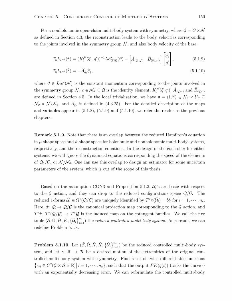
Chapter 5. Concurrent Control of Multi-body Systems 150
For a nonholonomic open-chain multi-body system with symmetry, where G = G×Nas defined in Section 4.3, the reconstruction leads to the body velocities corresponding
to the joints involved in the symmetry group N , and also body velocity of the base.
TnLn−1(n) = (KN1 (q1, q′))−1Ad∗(e,n)(ϑ)−
[A(q1,q′) B(q1,q′)
] [ ˙q1
q′
], (5.1.9)
ThLh−1(h) = −Aq1 ˙q1, (5.1.10)
where ϑ ∈ Lie∗(N ) is the constant momentum corresponding to the joints involved in
the symmetry group N , e ∈ Nϑ ⊆ Q is the identity element, KN1 (q, q′), A(q,q′) and B(q,q′)
are defined in Section 4.5. In the local trivialization, we have n = (k, n) ∈ Nϑ × Uϑ ⊆Nϑ × N /Nϑ, and Aq1 is defined in (4.3.25). For the detailed description of the maps
and variables appear in (5.1.8), (5.1.9) and (5.1.10), we refer the reader to the previous
chapters.
Remark 5.1.9. Note that there is an overlap between the reduced Hamilton’s equation
in µ-shape space and ϑ-shape space for holonomic and nonholonomic multi-body systems,
respectively, and the reconstruction equations. In the design of the controller for either
systems, we will ignore the dynamical equations corresponding the speed of the elements
of Q1/Gµ or N /Nϑ. One can use this overlap to design an estimator for some uncertain
parameters of the system, which is out of the scope of this thesis.
Based on the assumption CON3 and Proposition 5.1.3, Ui’s are basic with respect
to the G action, and they can drop to the reduced configurations space Q/G. The
reduced 1-forms Ui ∈ Ω1(Q/G) are uniquely identified by T ∗π(Ui) = Ui for i = 1, · · · , nc.Here, π : Q → Q/G is the canonical projection map corresponding to the G action, and
T ∗π : T ∗(Q/G) → T ∗Q is the induced map on the cotangent bundles. We call the five
tuple (S, Ω, H, K,Uinci=1
) the reduced controlled multi-body system. As a result, we can
redefine Problem 5.1.8.
Problem 5.1.10. Let (S, Ω, H, K,Uinci=1
) be the reduced controlled multi-body sys-
tem, and let γ : R → R be a desired motion of the extremities of the original con-
trolled multi-body system with symmetry. Find a set of twice differentiable functionsui ∈ C2(G × S × R)
∣∣ i = 1, · · · , nc
, such that the output FK(q(t)) tracks the curve γ
with an exponentially decreasing error. We can reformulate the controlled multi-body
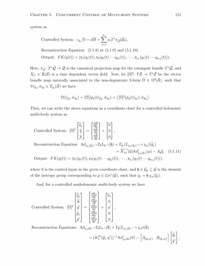
Chapter 5. Concurrent Control of Multi-body Systems 151
system as
Controlled System: ιXC Ω = dH +nc∑i=1
uiT∗πQ(Ui),
Reconstruction Equation: (5.1.8) or (5.1.9) and (5.1.10)
Output: FK(q(t)) = (r1(q1(t)), r2(q1(t) · · · q20(t)), · · · , rne(q1(t) · · · qne0(t))).
Here, πQ : T ∗Q → Q is the canonical projection map for the cotangent bundle T ∗Q, and
XC ∈ X(S) is a time dependent vector field. Now, let [Ω]] : T S → T ∗S be the vector
bundle map naturally associated to the non-degenerate 2-form Ω ∈ Ω2(S), such that
∀vpq , wpq ∈ Tpq(S) we have
Ω(vpq , wpq) = [Ω](pq)(vpq , wpq) =⟨[Ω]](pq)(vpq), wpq
⟩.
Then, we can write the above equations in a coordinate chart for a controlled holonomic
multi-body system as
Controlled System: [Ω]]
˙q1
q
p
=
∂H∂q1∂H∂q∂H∂p
+
0
u
0
,Reconstruction Equation: Adχµ(q1)−1ThLh−1(h) + Tq1(Lχµ(q1)−1 χµ)( ˙q1)
= K−1
11 (q)Ad∗χµ(q1)(µ)− Aq q, (5.1.11)
Output: FK(q(t)) = (r1(q1(t)), r2(q1(t) · · · q20(t)), · · · , rne(q1(t) · · · qne0(t))),
where u is the control input in the given coordinate chart, and h ∈ Gµ ⊆ G is the element
of the isotropy group corresponding to µ ∈ Lie∗(G), such that q1 = hχµ(q1).
And, for a controlled nonholonomic multi-body system we have
Controlled System: [Ω]]
˙q1
˙n
q′
˙p1
p′
=
∂Hϑ∂q1∂Hϑ∂n∂Hϑ∂q′
∂Hϑ∂p1
∂Hϑ∂p′
+
u1
0
u′
0
0
,
Reconstruction Equations: Adχϑ(n)−1TkLk−1(k) + Tn(Lχϑ(n)−1 χϑ)( ˙n)
= (KN1 (q1, q′))−1Ad∗χϑ(n)(ϑ)−
[A(q1,q′) B(q1,q′)
] [ ˙q1
q′
],

Chapter 5. Concurrent Control of Multi-body Systems 152
ThLh−1(h) = −Aq1 ˙q1, (5.1.12)
Output: FK(q(t)) = (r1(q1(t)), r2(q1(t) · · · q20(t)), · · · , rne(q1(t) · · · qne0(t))),
where u1 and u′ are the control input in the given coordinate chart, and h ∈ G ⊆ Q1
is an element of the subgroup of Q1, the embedding χϑ : Uϑ ⊆ N /Nϑ → N corresponds
to the local trivialization such that n = kχϑ(n) for the element k ∈ Nϑ, and Nϑ ⊆ N is
the isotropy group corresponding to ϑ ∈ Lie∗(N ). The equations (5.1.11) and (5.1.12)
formally define the control problem in the reduced phase space.
5.2 End-effector Pose and Velocity Error
5.2.1 Error Function
In this section we introduce a quadratic error function, based on an induced metric on
the output manifold R from a left-invariant metric on Pe. This error function represents
the distance between the actual output and the desired output of the system in the am-
bient manifold Pe. Different methods of defining error functions and their corresponding
gradients are discussed in Bullo’s thesis [12]. The definition of the error function adopted
in this thesis is due to its geometrical interpretation. But, the following development can
readily be applied to other definitions of the error function.
Definition 5.2.1. A smooth two variable function Er : R × R → R≥0 is a symmetric
error function on R, if ∀r1, r2 ∈ R we have Er(r1, r2) ≥ 0 and we have equality if and
only if r1 = r2.
Let ιR : R → Pe be the inclusion map, and let Ki (for i = 1, · · · , ne) be an arbitrary
left invariant Riemannian metric on SE(3) corresponding to the ith extremity. These
metrics induce a left invariant metric K := K1⊕ · · · ⊕Kne on Pe. Consider two elements
r1, r2 ∈ R and the one-parameter subgroup σ : R → Pe in Pe that connects ιR(r1) to
ιR(r2). We define the distance between r1 ∈ R and r2 ∈ R by the length of the portion
of σ that connects ιR(r1) ∈ Pe to ιR(r2) ∈ Pe in the ambient manifold. That is,
dis(r1, r2) =
∫ 1
0
√Kσ(s)
(dσ(s)
ds,dσ(s)
ds
)ds σ(0) = ιR(r1), σ(1) = ιR(r2)
=
∫ 1
0
√KeP
(σ−1(s)
dσ(s)
ds, σ−1(s)
dσ(s)
ds
)ds,

Chapter 5. Concurrent Control of Multi-body Systems 153
where s ∈ R is the curve parameter for σ, and eP is the identity element of Pe. Since
one-parameter subgroups are the integral curves of left invariant vector fields, we can
uniquely write the curve as
σ(s) = ιR(r1) exp(s exp−1(re)
),
where re := ιR(r1)−1ιR(r2) that is called output pose error. Consequently, we have
σ−1(s)dσ(s)
ds= exp−1(re),
which is a constant vector in Lie(Pe). As a result, we can simplify the above equation
dis(r1, r2) =√KeP (exp−1(re), exp−1(re)) =‖ exp−1(re) ‖KeP ,
where ‖ · ‖KeP is the induced norm on Lie(Pe) by the left invariant metric K. This length
is also equal to the length of the one-parameter subgroup that connects eP ∈ Pe to re.
It is easy to show that the error function defined by
Er(r1, r2) =1
2dis(r1, r2)2 =
1
2‖ exp−1(re) ‖2
KeP(5.2.13)
is a quadratic, smooth, symmetric error function on R.
Remark 5.2.2. Although it would have been natural to define the length of the geodesic
corresponding to the induced metric on R by K as the error function, the error function
defined by 5.2.13 is more efficient computationally.
We denote the exterior derivative of the error function with respect to the first and
second input of the function by d1 and d2, respectively. Also, let us use KP for the self-
adjoint positive definite map between Lie(Pe) and Lie∗(Pe) corresponding to the induced
metric on the Lie algebra. Then, for all vr1 ∈ Tr1R and wr2 ∈ Tr2R we have the following
equations:
〈d1Er(r1, r2), vr1〉 =1
2
⟨d1KeP
(exp−1(re), exp−1(re)
), vr1
⟩= −KeP
(exp−1(re),Θ(re)
−1AdιR(r2)−1(TιR(r1)RιR(r1)−1)(Tr1ιR)(vr1))
=⟨−KP exp−1(re),Θ(re)
−1AdιR(r2)−1(TιR(r1)RιR(r1)−1)(Tr1ιR)(vr1)⟩
=⟨−(T ∗r1ιR)(T ∗ιR(r1)RιR(r1)−1)Ad∗ιR(r2)−1(Θ(re)
−1)∗KP exp−1(re), vr1⟩,
(5.2.14)
〈d2Er(r1, r2), wr2〉 =1
2
⟨d2KeP
(exp−1(re), exp−1(re)
), wr2
⟩

Chapter 5. Concurrent Control of Multi-body Systems 154
= KeP(exp−1(re),Θ(re)
−1(TιR(r2)LιR(r2)−1)(Tr2ιR)(wr2))
=⟨KP exp−1(re),Θ(re)
−1(TιR(r2)LιR(r2)−1)(Tr2ιR)(wr2)⟩
=⟨(T ∗r2ιR)(T ∗ιR(r2)LιR(r2)−1)(Θ(re)
−1)∗KP exp−1(re), wr2⟩, (5.2.15)
where d1Er(r1, r2) ∈ T ∗r1R and d2Er(r1, r2) ∈ T ∗r2R. The map Θ(re) : Lie(P) → Lie(P)
defined by
Θ(re) =
∫ 1
0
Adexp(s exp−1(re))ds
is the linear map that appears in the tangent map of the exponential of Lie groups, which
was defined in the proof of Theorem 2.1.5 and calculated by (2.4.23) in Proposition 2.4.5
for SE(3). This map is invertible in an open neighbourhood of the identity element.
From now on, we always assume that re = ιR(r1)−1ιR(r2) belongs to a symmetric neigh-
bourhood of identity such that Θ(re) is invertible.
5.2.2 Velocity Error
The notion of connection on manifolds is usually used to linearly identify the tangent
spaces of the manifold at different base points, along a path. It is also used to define
the derivative of a vector field along a curve on the manifold, and consequently defining
the notion of parallel transport along a curve. A well-known example of connections on
manifolds is the affine connection on Riemannian manifolds. For Lie groups, one can
use the tangent to left or right translation maps to globally define a well-defined (trivial)
connection on Lie groups. In this way, we identify the tangent space at each element of
the Lie group with the Lie algebra of the Lie group. In this section we use the induced
connection on R by the right translation map of the Lie group Pe to define the output
velocity error of a controlled multi-body system.
For any r′1, r′2 ∈ Pe, let Tr′2R(r′2)−1r′1
: Tr′2Pe → Tr′1Pe be the tangent map of the right
translation by (r′2)−1r′1 that is a linear isomorphism between the tangent spaces Tr′1Pe and
Tr′2Pe. Recall that the canonical inclusion map and the projection map for the output
manifold R are denoted by ιR : R → Pe and r : Pe → R, respectively. We define the
linear isomorphism <(r1,r2) : Tr2R → Tr1R by
<(r1,r2) = (TιR(r1)r)(TιR(r2)RιR(r2)−1ιR(r1))(Tr2ιR) = (TιR(r1)r)(TιR(r2)Rr−1e
)(Tr2ιR),
(5.2.16)
which is a well-defined connection for any r2 ∈ R in a neighbourhood of r1 ∈ R. Note
that unlike the tangent map of the right translation on a Lie group, which globally defines
the trivial connection on a Lie group, the connection that is defined in (5.2.16) can only

Chapter 5. Concurrent Control of Multi-body Systems 155
make sense, locally. The size of the neighbourhood of r1, in which the above map is a
linear isomorphism, depends on the given projection map r.
Definition 5.2.3. Let γ1 : R → R and γ2 : R → R be two curves, and t ∈ R be their
curve parameter. We call
Ve(t) =d
dtγ1(t)−<(γ1(t),γ2(t))(
d
dtγ2(t)) =: γ1(t)−<(γ1(t),γ2(t))(γ2(t)) (5.2.17)
the output velocity error of a system.
Note that unlike the case of systems on linear spaces, where the velocity error can be
simply defined by subtracting the velocity of curves, in the case of systems on manifolds,
we need the notion of connection to define the velocity error. In the next section, we use
this notion to design control laws for controlled multi-body systems with symmetry.
Definition 5.2.4. A connection is called compatible with the error function, if ∀r1, r2 ∈ Rthe following equality holds [12]:
d2Er(r1, r2) = −<∗(r1,r2)d1Er(r1, r2). (5.2.18)
Corollary 5.2.5 ([12]). Let γ1 : R→ R and γ2 : R→ R be two curves. If the connection
is compatible with the error function, then
d
dtEr(γ1(t), γ2(t)) = 〈d1Er(γ1(t), γ2(t)), Ve(t)〉 . (5.2.19)
Proposition 5.2.6. If R is the right translation of a Lie subgroup of Pe by an element
r′0 ∈ Pe, then the connection in (5.2.16) is compatible with the error function in (5.2.13).
Proof. It is easy to check that for all r1, r2 ∈ R the connection <(r1,r2) is compatible with
Er(r1, r2), if ∀vr2 ∈ Tr2R we have
(TιR(r2)RιR(r2)−1ιR(r1)
)Tr2ιR(vr2) ∈ Tr1ιR(Tr1R),
since the tangent of the projection map T r is identity on Tr1ιR(Tr1R).
We claim that the above condition is satisfied if R = Gr′0, where G is a Lie subgroup
of SE(3). Let g1, g2 ∈ G such that r1 = g1r′0 and r2 = g2r
′0. Then, we have
Tr1R = (Tg1G)r′0 = Lie(G)g1r′0 = Lie(G)r1.
Similarly, it is easy to show that Tr2R = Lie(G)r2. As a result, ∀vr2 ∈ Tr2R there exists
a ξ ∈ Lie(G), such that vr2 = ξr2. If we apply the connection in (5.2.16) to this vector,
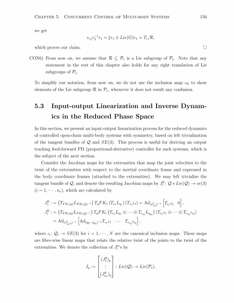
Chapter 5. Concurrent Control of Multi-body Systems 156
we get
vr2r−12 r1 = ξr1 ∈ Lie(G)r1 = Tr1R,
which proves our claim.
CON6) From now on, we assume that R ⊆ Pe is a Lie subgroup of Pe. Note that any
statement in the rest of this chapter also holds for any right translation of Lie
subgroups of Pe.
To simplify our notation, from now on, we do not use the inclusion map ιR to show
elements of the Lie subgroup R in Pe, whenever it does not result any confusion.
5.3 Input-output Linearization and Inverse Dynam-
ics in the Reduced Phase Space
In this section, we present an input-output linearization process for the reduced dynamics
of controlled open-chain multi-body systems with symmetry, based on left trivialization
of the tangent bundles of Q and SE(3). This process is useful for deriving an output
tracking feed-forward PD (proportional-derivative) controller for such systems, which is
the subject of the next section.
Consider the Jacobian maps for the extremities that map the joint velocities to the
twist of the extremities with respect to the inertial coordinate frame and expressed in
the body coordinate frames (attached to the extremities). We may left trivialize the
tangent bundle of Q, and denote the resulting Jacobian maps by J0i : Q×Lie(Q)→ se(3)
(i = 1, · · · , ne), which are calculated by
J01 : =
(TFK1(q)LFK1(q)−1
)TqFK1 (Te1Lq1) (Te1ι1) = Ad(r0
1,0)−1
[Te1ι1 0
],
J0i : =
(TFKi(q)LFKi(q)−1
)TqFKi
(Te1Lq1 ⊕ · · · ⊕ Tei0Lqi0
)(Te1ι1 ⊕ · · · ⊕ Tei0 ιi0)
= Ad(r0i0,0
)−1
[Ad(q2···qi0 )−1Te1ι1 · · · Tei0 ιi0
],
where ιi : Qi → SE(3) for i = 1, · · · , N are the canonical inclusion maps. These maps
are fibre-wise linear maps that relate the relative twist of the joints to the twist of the
extremities. We denote the collection of J0i ’s by
Jq :=
(J0
1 )q...
(J0ne)q
: Lie(Q)→ Lie(Pe).
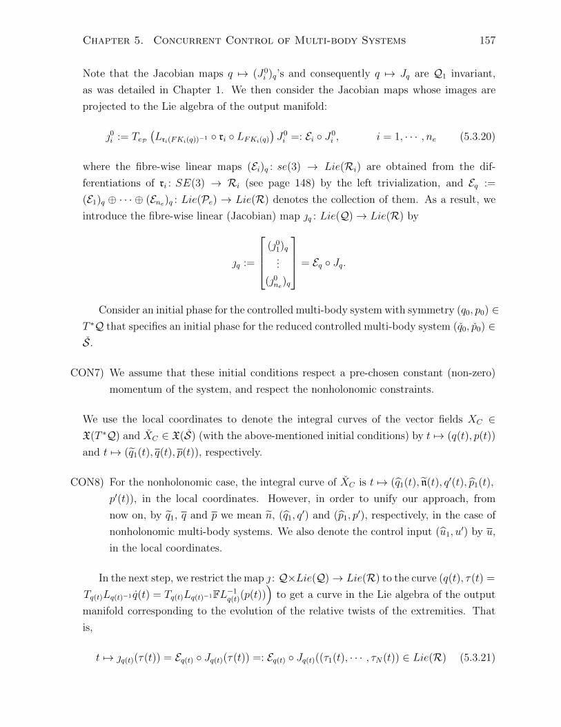
Chapter 5. Concurrent Control of Multi-body Systems 157
Note that the Jacobian maps q 7→ (J0i )q’s and consequently q 7→ Jq are Q1 invariant,
as was detailed in Chapter 1. We then consider the Jacobian maps whose images are
projected to the Lie algebra of the output manifold:
0i := TeP(Lri(FKi(q))−1 ri LFKi(q)
)J0i =: Ei J0
i , i = 1, · · · , ne (5.3.20)
where the fibre-wise linear maps (Ei)q : se(3) → Lie(Ri) are obtained from the dif-
ferentiations of ri : SE(3) → Ri (see page 148) by the left trivialization, and Eq :=
(E1)q ⊕ · · · ⊕ (Ene)q : Lie(Pe) → Lie(R) denotes the collection of them. As a result, we
introduce the fibre-wise linear (Jacobian) map q : Lie(Q)→ Lie(R) by
q :=
(01)q
...
(0ne)q
= Eq Jq.
Consider an initial phase for the controlled multi-body system with symmetry (q0, p0) ∈T ∗Q that specifies an initial phase for the reduced controlled multi-body system (q0, p0) ∈S.
CON7) We assume that these initial conditions respect a pre-chosen constant (non-zero)
momentum of the system, and respect the nonholonomic constraints.
We use the local coordinates to denote the integral curves of the vector fields XC ∈X(T ∗Q) and XC ∈ X(S) (with the above-mentioned initial conditions) by t 7→ (q(t), p(t))
and t 7→ (q1(t), q(t), p(t)), respectively.
CON8) For the nonholonomic case, the integral curve of XC is t 7→ (q1(t), n(t), q′(t), p1(t),
p′(t)), in the local coordinates. However, in order to unify our approach, from
now on, by q1, q and p we mean n, (q1, q′) and (p1, p
′), respectively, in the case of
nonholonomic multi-body systems. We also denote the control input (u1, u′) by u,
in the local coordinates.
In the next step, we restrict the map : Q×Lie(Q)→ Lie(R) to the curve (q(t), τ(t) =
Tq(t)Lq(t)−1 q(t) = Tq(t)Lq(t)−1FL−1q(t)(p(t))
)to get a curve in the Lie algebra of the output
manifold corresponding to the evolution of the relative twists of the extremities. That
is,
t 7→ q(t)(τ(t)) = Eq(t) Jq(t)(τ(t)) =: Eq(t) Jq(t)((τ1(t), · · · , τN(t)) ∈ Lie(R) (5.3.21)

Chapter 5. Concurrent Control of Multi-body Systems 158
In the holonomic case the first entry of this map τ1(t) = Tq1(t)Lq(t)−1 q1(t) is the relative
twist of the first body with respect to the inertial coordinate frame and expressed in
the body coordinate frame, which is the outcome of the reconstruction equation (5.1.8).
That is,
τ1(t) = K−1
11 (q(t))Ad∗χµ(q1(t))(µ)− Aq(t)q(t). (5.3.22)
Based on (5.1.10), for a nonholonomic open-chain multi-body system with symmetry
we have
τ1(t) = (h(t)χ(q1(t)))−1(h(t)χ(q1(t)) + h(t)Tχ( ˙q1(t))
)= Adχ(q1(t))−1
(h−1(t)h(t)
)+ χ(q1(t))−1Tχ( ˙q1(t))
= −Adχ(q1(t))−1
(Aq1(t)
˙q1(t))
+ χ(q1(t))−1Tχ( ˙q1(t)). (5.3.23)
Also, if the relative configuration manifold of a joint appears in the symmetry group N ,
we have the same equation as in (5.3.22) for the relative twist of the corresponding joint.
Let [Ω]] : T S → T ∗S be the vector bundle map corresponding to the 2-form Ω ∈Ω2(S), in the dynamical equations of a reduced controlled holonomic or nonholonomic
open-chain multi-body system. Consider rearranging of the coordinate variables of non-
holonomic systems based on CON8, then for both the holonomic and nonholonomic case
the momenta in the reduced phase space S are denoted by the coordinates pi. According
to the notation of (3.2.27) and (Eq.Ham.Non.Coor) we have
ι∂/∂piΞµ = 0,
ι∂/∂pi(Ξϑ − Ξϑ) = 0.
As a result, it is easy to check that ∀(q, p) ∈ Sq in the reduced phase space [Ω]]((q, p))
has the following form:
[Ω]](q, p) =
[Ω]]11(q, p) [Ω]]12(q, p) 0
−([Ω]]12(q, p))T [Ω]]22(q, p) −id0 id 0
,and the inverse of it ([Ω]])−1 : T ∗S → T S has the following form:
([Ω]](q, p))−1 =
([Ω]]11)−1 0 −([Ω]]11)−1[Ω]]12
0 0 id
−([Ω]]12)T ([Ω]]11)−1 −id [Ω]]22 + ([Ω]]12)T ([Ω]]11)−1[Ω]]12
.

Chapter 5. Concurrent Control of Multi-body Systems 159
Therefore, we can write the speed of the integral curve of the controlled holonomic or
nonholonomic open-chain multi-body system as: ˙q1
q
p
= ([Ω]](q(t), p(t)))−1
∂H∂q1
∂H∂q
+ u∂H∂p
=
([Ω]]11)−1 0 −([Ω]]11)−1[Ω]]12
0 0 id
−([Ω]]12)T ([Ω]]11)−1 −id [Ω]]22 + ([Ω]]12)T ([Ω]]11)−1[Ω]]12
∂H∂q1
∂H∂q
+ u∂H∂p
=
([Ω]]11)−1 ∂H
∂q1−(
([Ω]]11)−1[Ω]]12
)∂H∂p
∂H∂p
−(
([Ω]]12)T ([Ω]]11)−1)∂H∂q1− ∂H
∂q− u+
([Ω]]22 + ([Ω]]12)T ([Ω]]11)−1[Ω]]12
)∂H∂p
.(5.3.24)
Based on the first two equations in (5.3.24) we can write
˙q1(t) = ([Ω]]11)−1∂H
∂q1
−(
([Ω]]11)−1[Ω]]12
) ∂H∂p
=: q(q(t), p(t)), (5.3.25)
q(t) =∂H
∂p=: q(q(t), p(t)), (5.3.26)
By substituting these equations in (5.3.22) and (5.3.23) (and any reconstruction equation
due to the second step of the reduction of nonholonomic systems) we obtain the following
relations for holonomic and nonholonomic cases, respectively:
τ1(t) = K−1
11 (q(t))Ad∗χµ(q1(t))(µ)− Aq(t)q(q(t), p(t)).
and
τ1(t) = −Adχ(q1(t))−1
(Aq1(t)q1((q(t), p(t)))
)+ χ(q1(t))−1Tχ(q1(q(t), p(t))),
where q1 : S → T (Q1/G) specifies the components of XC ∈ X(S) in T (Q1/G) as a
portion of the components of q. In general, we can write τ(t) =: τ(q(t), p(t)), where
the function τ : S → Lie(Q) is defined based on (5.3.25), (5.3.26) and reconstruction
equations. Therefore, the curve in (5.3.21) can be rewritten as
t 7→ q(t) τ(q(t), p(t))) ∈ Lie(R),

Chapter 5. Concurrent Control of Multi-body Systems 160
where we have τ : G × S → Lie(R). Taking the derivative of this curve with respect
to time, we obtain a curve in TLie(R) ∼= Lie(R):
t 7→ d
dt
(q(t) τ(q(t), p(t))
)=
(∂q(t)∂q
q(t)
)τ(q(t), p(t)) + q(t)
(∂τ
∂q˙q(t) +
∂τ
∂p˙p(t)
)=
(∂q(t)∂q
(TeLq(t)τ(q(t), p(t))
))τ(q(t), p(t)) + q(t)
(∂τ
∂q˙q(t) +
∂τ
∂p˙p(t)
)=
(∂q(t)∂q
(TeLq(t)τ(q(t), p(t))
))τ(q(t), p(t))
+ q(t)
(∂τ
∂q
[q(q(t), p(t))
q(q(t), p(t))
]+∂τ
∂p(p(q(t), p(t))− u)
)∈ Lie(R),
(5.3.27)
where the last line is the consequence of substituting (5.3.25) and (5.3.26) in the equation,
and the map p is defined based on the last equation of (5.3.24):
p(q(t), p(t)) = −(
([Ω]]12)T ([Ω]]11)−1) ∂H∂q1
− ∂H
∂q+(
[Ω]]22 + ([Ω]]12)T ([Ω]]11)−1[Ω]]12
) ∂H∂p
.
(5.3.28)
Equation (5.3.27) is the input-output linearized form in the reduced phase space of a
generic holonomic or nonholonomic open-chain multi-body system with multi-d.o.f. joints
and non-zero momentum. The input-output linearization method presented in this sec-
tion generalizes different approaches to the input-output linearization of underactuated,
holonomic and nonholonomic multi-body systems used, e.g., in [2, 5, 28, 34, 60, 61],
to derive nonlinear control laws. Equation (5.3.27) holds for any holonomic open-chain
multi-body system with non-abelian symmetry group and non-zero momentum, and also
it holds for Chaplygin systems with underactuated joints.
In (5.3.27), u is going to be designed such that the output of the controlled holonomic
or nonholonomic open-chain multi-body system follows the desired trajectory t 7→ γ(t).
As a result, we solve the inverse dynamics problem for a free-base, open-chain multi-body
system with symmetry by equating the curve in (5.3.27) and ddt
(γ−1(t)γ(t)):
d
dt(r−1(t)r(t)) =
d
dt
(q(t) τ(q(t), p(t))
)=
d
dt
(γ−1(t)γ(t)
).
Now, we use the last line of (5.3.27) to find the solution for the inverse dynamics problem,
by solving for u in the reduced phase space.
u(q(t), p(t), γ(t), γ(t), γ(t)) =
(q(t)
∂τ
∂p
)−1((∂q(t)∂q
(TeLq(t)τ(q(t), p(t))
))τ(q(t), p(t))

Chapter 5. Concurrent Control of Multi-body Systems 161
+q(t)∂τ
∂q
[q(q(t), p(t))
q(q(t), p(t))
]− d
dt
(γ−1(t)γ(t)
))+ p(q(t), p(t)).
(5.3.29)
Note that (5.3.29) matches with equation (17) in [28] in a special case where the total
momentum of the system is equal to zero and there is no nonholonomic constraints at
the base. Also, the formulation in [28] is based on a specific parametrization of the
output manifold of the system. Therefore, (5.3.29) can be considered as a coordinate-
independent generalization of the inverse dynamics solution in the reduced phase space
for non-zero momentum subject to holonomic or nonholonomic constraints.
Remark 5.3.1. The matrix q(t)∂τ∂p
is square if the dimension of the control codistribution
F is equal to the dimension of the output manifold, i.e., no = nc. In case no < nc, we
can either choose u amongst all possible solutions by, for example, optimizing a function
along the trajectories of the system, or use a pseudo inverse matrix in the above equation.
Remark 5.3.2. Note that since the Legendre transformation is invertible for the re-
duced open-chain multi-body system with symmetry, the matrix ∂τ∂p
is always full rank.
Furthermore, for a feasible desired trajectory t 7→ γ(t) the Jacobian q(t) is also full rank.
Therefore, the inverse dynamics problem in the reduced phase space has a unique solu-
tion u (or the matrix q(t)∂τ∂p
is invertible), if no = nc and the desired trajectory t 7→ γ(t)
is feasible.
CON9) In the next section, we assume that the dimension of the output manifold is equal to
the number of control inputs of a controlled holonomic or nonholonomic open-chain
multi-body system, i.e., no = nc.
5.4 An Output-tracking Feed-forward
Servo Controller
In this section, under the dimensional assumption CON9 and the feasibility of the desired
trajectory t 7→ γ(t), we develop an output tracking feed-forward servo controller for a
generic open-chain multi-body system with symmetry. The system can include multi-
d.o.f. joints and can be subject to holonomic or nonholonomic constraints. Also, for the
holonomic case the total momentum of the system can be non-zero. In this process, we use
the definition of the error function and velocity error of the system output introduced in
Section 5.2. Consequently, we show that the developed controller exponentially stabilizes
the closed-loop system using Lyapunov function t 7→ VL(r(t), r(t), γ(t), γ(t)) ∈ R.

Chapter 5. Concurrent Control of Multi-body Systems 162
Definition 5.4.1 ([12]). Let t 7→ r(t) := FK(q(t)) ∈ R denote the output of a controlled
holonomic or nonholonomic, open-chain multi-body system, and let t 7→ γ(t) ∈ R be a
feasible desired output trajectory. The desired trajectory γ
i) is Lyapunov stable with Lyapunov function t 7→ VL(r(t), r(t), γ(t), γ(t)) ∈ R, if
VL(t) ≤ VL(0) from all initial conditions (r(0), r(0)).
ii) is exponentially stable with Lyapunov function t 7→ VL(r(t), r(t), γ(t), γ(t)) ∈ R, if
there exist two positive constants δ1 and δ2 such that VL(t) ≤ δ1VL(0)eδ2t from all
initial conditions (r(0), r(0)).
Theorem 5.4.2. Consider the controlled holonomic or nonholonomic, open-chain multi-
body system in (5.1.11) or (5.1.12), and let the curve t 7→ γ(t) ∈ R be a twice differ-
entiable feasible trajectory in the output manifold that satisfies the assumption CON4.
Also, let Er : R × R → R≥0 be the error function in (5.2.13) and < be its compat-
ible connection (assuming CON6), defined by (5.2.16). Let KP : Lie(R) → Lie∗(R),
KD : Lie(R) → Lie∗(R) and I : Lie(R) → Lie∗(R) be self-adjoint positive-definite ten-
sors, such that I induces a norm on Lie(R) denoted by ‖ · ‖I. Under the condition
CON9 the control input in the reduced phase space is
u(q, p, γ, γ, γ) =
(q∂τ
∂p
)−1((
∂q∂q
(TeLq τ(q, p))
)τ(q, p) + q
∂τ
∂q
[q(q, p)
q(q, p)
]− ν
)+ p(q, p),
(5.4.30)
where we have the control law as:
ν = νPD + νFF , (5.4.31)
νPD = −I−1T ∗ePLr(t) (d1Er(r, γ))− I−1KDve(r, γ, r, γ), (5.4.32)
νFF = ad(r−1r)Ad(r−1γ)
(γ−1γ
)+ Ad(r−1γ)
(d
dt
(γ−1γ
))(5.4.33)
where r(t) := FK(q(t)) ∈ R is the output of the system, and
ve(r, γ, r, γ) := r−1r − r−1<(r,γ)(γ) = r−1r − Ad(r−1γ)(γ−1γ) (5.4.34)
is the left translated output velocity error to Lie(R). Then, the desired trajectory t 7→ γ(t)
is Lyapunov stable with the Lyapunov function VL : R→ R≥0:
VL(t) = Er(r, γ) +1
2〈Ive(r, γ, r, γ), ve(r, γ, r, γ)〉 . (5.4.35)
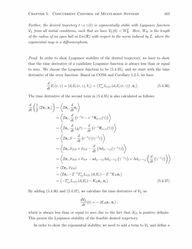
Chapter 5. Concurrent Control of Multi-body Systems 163
Further, the desired trajectory t 7→ γ(t) is exponentially stable with Lyapunov function
VL from all initial conditions, such that we have VL(0) < W 2R. Here, WR is the length
of the radius of an open ball in Lie(R) with respect to the norm induced by I, where the
exponential map is a diffeomorphism.
Proof. In order to show Lyapunov stability of the desired trajectory, we have to show
that the time derivative of a candidate Lyapunov function is always less than or equal
to zero. We choose the Lyapunov function to be (5.4.35), and we start with the time
derivative of the error function. Based on CON6 and Corollary 5.2.5, we have
d
dtEr(r, γ) = 〈d1Er(r, γ), Ve〉 =
⟨T ∗ePLr(t) (d1Er(r, γ)) , ve
⟩. (5.4.36)
The time derivative of the second term in (5.4.35) is also calculated as follows:
d
dt
(1
2〈Ive, ve〉
)=
⟨Ive,
d
dtve
⟩=
⟨Ive,
d
dt
(r−1r − r−1<(r,γ)(γ)
)⟩=
⟨Ive,
d
dt(q τ)− d
dt
(r−1<(r,γ)(γ)
)⟩=
⟨Ive, ν −
d
dt
(r−1(γ)γ−1r
)⟩=
⟨Ive, νPD + νFF −
d
dt
(Ad(r−1γ)(γ
−1γ))⟩
=
⟨Ive, νPD + νFF − ad(r−1r)Ad(r−1γ)
(γ−1γ
)+ Ad(r−1γ)
(d
dt
(γ−1γ
))⟩= 〈Ive, νPD〉
=⟨Ive,−I−1T ∗ePLr(t) (d1Er)− I−1KDve
⟩=⟨−T ∗ePLr(t) (d1Er)−KDve, ve
⟩. (5.4.37)
By adding (5.4.36) and (5.4.37), we calculate the time derivative of VL as:
dVLdt
(t) = −〈KDve, ve〉 ,
which is always less than or equal to zero due to the fact that KD is positive definite.
This proves the Lyapunov stability of the feasible desired trajectory.
In order to show the exponential stability, we need to add a term to VL and define a

Chapter 5. Concurrent Control of Multi-body Systems 164
new Lyapunov function VL : R→ R≥0:
VL(t) := Er(r, γ) +1
2〈Ive(r, γ, r, γ), ve(r, γ, r, γ)〉+ δ
d
dtEr(r, γ),
where we have to find δ > 0 such that VL is positive definite, i.e., VL is greater than
or equal to zero and it is zero if and only if Er(r, γ) = 0 and ve(r, γ, r, γ) = 0. Let
re(t) = r(t)−1γ(t):
VL(t) = Er +1
2〈Ive, ve〉+ δ
⟨T ∗ePLr (d1Er) , ve
⟩=
1
2
⟨KP exp−1(re), exp−1(re)
⟩+
1
2〈Ive, ve〉+ δ
⟨T ∗ePLr (d1Er) , ve
⟩=
1
2
⟨KP exp−1(re), exp−1(re)
⟩+
1
2〈Ive, ve〉 − δ
⟨Ad∗
r−1e
(Θ(re)−1)∗KP exp−1(re), ve
⟩.
From the proof of Lyapunov stability of the closed loop t 7→ γ(t), we have
VL(t) ≤ VL(0) =: W0 =⇒ Er(r, γ) ≤ W0, ‖ ve(r, γ, r, γ) ‖I≤ W0.
We consider the induced norm by KeP and I on the space of all automorphisms of Lie(R),
as a vector space. For any linear map = : Lie(R)→ Lie(R), this induced norm is defined
by
‖ = ‖I := max ‖ =ξ ‖I | ξ ∈ Lie(R), ‖ ξ ‖I= 1 ,
for I, and similarly we can define the norm, which is induced by KeP . Since the er-
ror function is bounded by the Lyapunov stability and re ∈ R is assumed to be in a
neighbourhood of the identity where Θ(re) is invertible, ∀t ∈ R we have the following
bounds:
‖ Adr−1e‖I ≤ sup
‖ Adr−1
e‖I∣∣ re ∈ R, ‖ exp−1(re) ‖KeP≤
√W0
= W1,
‖ Θ(re)−1 ‖I ≤ sup
‖ Θ(re)
−1 ‖I∣∣ re ∈ R, ‖ exp−1(re) ‖KeP≤
√W0
= W2.
As the result of these bounds,
VL(t) ≥ 1
2‖ exp−1(re) ‖2
KeP+
1
2‖ ve ‖2
I −δ ‖ exp−1(re) ‖KeP ‖ Θ(re)−1Adr−1
eve ‖I
≥ 1
2‖ exp−1(re) ‖2
KeP+
1
2‖ ve ‖2
I
− δ ‖ Adr−1e‖I‖ Θ(re)
−1 ‖I‖ exp−1(re) ‖KeP ‖ ve ‖I
≥ 1
2‖ exp−1(re) ‖2
KeP+
1
2‖ ve ‖2
I −δW1W2 ‖ exp−1(re) ‖KeP ‖ ve ‖I

Chapter 5. Concurrent Control of Multi-body Systems 165
=1
2
[‖ exp−1(re) ‖KeP
‖ ve ‖I
]T [1 −δW1W2
−δW1W2 1
][‖ exp−1(re) ‖KeP
‖ ve ‖I
]
=:1
2
[‖ exp−1(re) ‖KeP
‖ ve ‖I
]TW
[‖ exp−1(re) ‖KeP
‖ ve ‖I
],
where, W is a positive definite matrix if 0 < δ < 1√W1W2
. Therefore, for any δ in this
range, VL is a well-defined Lyapunov function.
Now, to calculate the time derivative of VL(t) we only need to take the derivative of
the term ddtEr(r, γ):
d
dt
(d
dtEr(r, γ)
)=
d
dt
⟨T ∗ePLr (d1Er) , ve
⟩= − d
dt
⟨Ad∗
r−1e
(Θ(re)−1)∗KP exp−1(re), ve
⟩= − d
dt
⟨KP exp−1(re),Θ(re)
−1Adr−1eve⟩
= −⟨KP
d
dt
(exp−1(re)
),Θ(re)
−1Adr−1eve
⟩−⟨KP exp−1(re),
d
dt
(Θ(re)
−1Adr−1eve)⟩
.
In the following, we calculate the terms appeared in the above equation.⟨KP
d
dt
(exp−1(re)
),Θ(re)
−1Adr−1eve
⟩=⟨KPΘ(re)
−1TePLr−1ere,Θ(re)
−1Adr−1eve⟩
= −⟨KPΘ(re)
−1Adr−1eve,Θ(re)
−1Adr−1eve⟩
= − ‖ Θ(re)−1Adr−1
eve ‖2
KeP, (5.4.38)
since we have
re =d
dt
(r−1γ)
)= −r−1rr−1γ + r−1γ = −
(r−1r − r−1γγ−1r
)re
= −TePRre
(r−1r − r−1<(r,γ)(γ)
)= −TePRre(ve).
And,
d
dt
(Θ(re)
−1Adr−1eve)
=
(∂Θ−1
∂rere
)Adr−1
e(ve)−Θ−1Adr−1
eadrer−1
e(ve) + Θ−1Adr−1
e(ve)
=
(∂Θ−1
∂re(−vere)
)Adr−1
e(ve)−Θ−1Adr−1
eadve(ve) + Θ−1Adr−1
e(νPD)
= −(∂Θ−1
∂re(vere)
)Adr−1
e(ve) + Θ−1Adr−1
e(νPD)
= −(∂Θ−1
∂re(vere)
)Adr−1
e(ve)−Θ−1Adr−1
e
(I−1T ∗ePLr (d1Er) + I−1KDve
)

Chapter 5. Concurrent Control of Multi-body Systems 166
= −(∂Θ−1
∂re(vere)
)Adr−1
e(ve)
+ Θ−1Adr−1e
(I−1Ad∗
r−1e
(Θ(re)−1)∗KP exp−1(re)− I−1KDve
),
(5.4.39)
which is the result of the following equalities:
re = −vere,
ve = νPD,
d
dtAdr−1
e(η) =
d
dt
(r−1e ηre
)= −r−1
e rer−1e ηre + r−1
e ηre = r−1e
(ηrer
−1e − rer−1
e η)re
= −Adr−1e
adrer−1e
(η),
where in the last equality η is an element of Lie(R). Therefore, by (5.4.38) and (5.4.39)
we have
d
dt
(d
dtEr(r, γ)
)= ‖ Θ(re)
−1Adr−1eve ‖2
KeP
+
⟨KP exp−1(re),
(∂Θ−1
∂re(vere)
)Adr−1
e(ve)
⟩−⟨
Ad∗r−1e
(Θ(re)−1)∗KP exp−1(re), I−1Ad∗
r−1e
(Θ(re)−1)∗KP exp−1(re)
⟩+⟨KP exp−1(re),Θ
−1Adr−1eI−1KDve
⟩.
Based on the norm equivalence inequality and since we have the bounds ‖ Adr−1e‖I≤ W1
and ‖ Θ(re)−1 ‖I≤ W2, there exists W3 > 0 such that⟨
Ad∗r−1e
(Θ(re)−1)∗KP exp−1(re), I−1Ad∗
r−1e
(Θ(re)−1)∗KP exp−1(re)
⟩=‖ Ad∗
r−1e
(Θ(re)−1)∗KP exp−1(re) ‖2
I
≥ W3 ‖ KP exp−1(re) ‖2KeP
= W3 ‖ exp−1(re) ‖2KeP
,
(5.4.40)
wherever we have an element of Lie∗(R) inside the norm we mean the naturally induced
norm by a metric on Lie∗(R). Also, we have the following inequalities:
‖ Θ(re)−1Adr−1
eve ‖2
KeP≤ W4 ‖ ve ‖2
I , (5.4.41)⟨KP exp−1(re),
(∂Θ−1
∂re(vere)
)Adr−1
e(ve)
⟩≤ W5 ‖ ve ‖I‖ exp−1(re) ‖KeP , (5.4.42)

Chapter 5. Concurrent Control of Multi-body Systems 167
⟨KP exp−1(re),Θ
−1Adr−1eK−1P KDve
⟩≤ W6 ‖ ve ‖I‖ exp−1(re) ‖KeP , (5.4.43)
where W4,W5,W6 > 0 are three positive real numbers. The inequalities in (5.4.40),
(5.4.41), (5.4.42) and (5.4.43) yields to
d
dt
(d
dtEr(r, γ)
)≤
− 1
2
[‖ exp−1(re) ‖KeP
‖ ve ‖I
]T [2W3 −(W5 +W6)
−(W5 +W6) −2W4
][‖ exp−1(re) ‖KeP
‖ ve ‖I
]
=: −1
2
[‖ exp−1(re) ‖KeP
‖ ve ‖I
]TW
[‖ exp−1(re) ‖KeP
‖ ve ‖I
],
where W is a symmetric matrix. As a result, we have
d
dtVL(t) ≤
− 1
2
[‖ exp−1(re) ‖KeP
‖ ve ‖I
]T [2δW3 −δ(W5 +W6)
−δ(W5 +W6) −2(δW4 −W6)
][‖ exp−1(re) ‖KeP
‖ ve ‖I
]
=: −1
2
[‖ exp−1(re) ‖KeP
‖ ve ‖I
]TW
[‖ exp−1(re) ‖KeP
‖ ve ‖I
]. (5.4.44)
It is easy to check that if
0 < δ <4W3W6
(W5 +W6)2 + 4W3W4
,
then W is a symmetric positive-definite matrix. Therefore, for any positive δ less than
the smaller of 1√W1W2
and 4W3W6
(W5+W6)2+4W3W4VL is a Lyapunov function and (5.4.44) holds.
Until this step, we have proved the asymptotic stability of the desired feasible trajectory
t 7→ γ(t) ∈ R.
In the final step, we show that in fact this trajectory is exponential stable. Consider
the Lyapunov function VL for an appropriate δ. We have
VL(t) ≤ 1
2‖ exp−1(re) ‖2
KeP+
1
2‖ ve ‖2
I +δW1W2 ‖ exp−1(re) ‖KeP ‖ ve ‖I
=1
2
[‖ exp−1(re) ‖KeP
‖ ve ‖I
]T [1 δW1W2
δW1W2 1
][‖ exp−1(re) ‖KeP
‖ ve ‖I
]

Chapter 5. Concurrent Control of Multi-body Systems 168
=:1
2
[‖ exp−1(re) ‖KeP
‖ ve ‖I
]TW ′[‖ exp−1(re) ‖KeP
‖ ve ‖I
],
whereW ′ is a symmetric positive definite matrix. Using the norm equivalence inequality,
there exists a positive number δ such that
d
dtVL(t) ≤ −1
2
[‖ exp−1(re) ‖KeP
‖ ve ‖I
]TW
[‖ exp−1(re) ‖KeP
‖ ve ‖I
]
≤ −δ2
[‖ exp−1(re) ‖KeP
‖ ve ‖I
]TW ′[‖ exp−1(re) ‖KeP
‖ ve ‖I
]≤ −δ VL(t).
Based on this inequality, VL(t) ≤ VL(0)e−δt. Consequently, there exists a positive number
δ such that
VL(t) =1
2
[‖ exp−1(re) ‖KeP
‖ ve ‖I
]T [1 0
0 1
][‖ exp−1(re) ‖KeP
‖ ve ‖I
]
≤ δ
2
[‖ exp−1(re) ‖KeP
‖ ve ‖I
]TW
[‖ exp−1(re) ‖KeP
‖ ve ‖I
]≤ δVL(t) ≤ δVL(0)e−δt ≤ 2δVL(0)e−δt,
where the last inequality holds due to the fact that VL(0) ≤ 2VL(0).
Remark 5.4.3. Theorem 5.4.2 presents an output tracking, feed-forward PD controller
in the reduced phase space that exponentially stabilizes the closed-loop generic holonomic
or nonholonomic multi-body system. The control input is a function of the joint displace-
ments, including those of the unactuated joints eliminated in the reduction process, and
the velocities of the actuated joints.
Remark 5.4.4. The controller input in (5.4.30) is in the reduced space. In order to
find the control input for the original system in (5.1.6), we have to first express u in the
reduced basis for the control directions, i.e.Uinci=1
, then we have to lift the result to
the original phase space of the system. That is,
u =:nc∑i=1
uiUi =nc∑i=1
uiUi,
where Ui = T ∗π(Ui).
Figure 5.4 depicts the block diagram of the proposed control scheme. In this diagram,

Chapter 5. Concurrent Control of Multi-body Systems 169
g is an element of the symmetry group G, and r′, r′ correspond to the actual motion of
the robot. Also, we have
νP = −I−1T ∗ePLr(t) (d1Er(r, γ)) = I−1Ad∗r−1e
(Θ(re)−1)∗KP exp−1(re),
νD = −I−1KDve(r, γ, r, γ) = −I−1KD(r−1r − Adre(γ
−1γ)),
νFF = ad(r−1r)Adre(γ−1γ
)+ Adre
(d
dt
(γ−1γ
))= ad(r−1r)Adre
(γ−1γ
)+ Adre
(γ−1γ − (γ−1γ)(γ−1γ)
)
In Theorem 5.4.2, we introduce a feed-forward PD controller at the output of a generic
controlled open-chain multi-body system. We used the group structure of the output
manifold to define the pose and velocity error for the extremities, and consequently, to
construct this controller. As a result, the controller, i.e., ν, is dependent on the group
structure of the output manifold. For this controller, the behaviour of the closed-loop
system can be presented in the form of the following set of coupled differential equations:
d
dt(r−1r) = νFF + νP + νD
γ−1γ − (γ−1γ)(γ−1γ)
γ−1γ
re = r−1γ
νFF
νD
νP
∑u(g, q, p, ν) ROBOT
FK(g, q)
(g, q, p)
(5.1.8)OR
(5.1.9) & (5.1.10)
p(q1, q, q)
q1
γ
γ
γ
g
q q
r
r′
r′
r−1r
Figure 5.1: Feed-forward servo control for a generic free-base, open-chain multi-bodysystem

Chapter 5. Concurrent Control of Multi-body Systems 170
=d
dt(Adre(γ
−1γ))− Ad∗r−1e
(Θ(re)−1)∗KP exp−1(re)−KD
(r−1r − Adre(γ
−1γ)),
where we assume that the linear map I : Lie(R) → Lie∗(R), which is used to define
Lyapunov function, is the identity matrix in a basis for the Lie algebra of R and its dual.
This simplification helps illustrating the behaviour of the closed-loop system. By some
manipulation, we get the following set of coupled differential equations for the output
error (re = r−1γ):
d
dt(rer
−1e ) +KD(rer
−1e ) + Ad∗
r−1e
(Θ(re)−1)∗KP exp−1(re) = 0.
Now by appropriately choosing the self-adjoint tensors KP and KD, we can achieve a
desired performance of the closed-loop system.
If the output manifold of the system is an abelian subgroup of Pe, the above differential
equation can be simplified to the familiar second order linear differential equation. Then
by choosing diagonal matrices for KP and KD we can decouple the differential equations
representing the behaviour of the closed-loop system, and we can explicitly design the
controller to achieve any desired performance of the system. In this case, the output
error is simply the difference between the desired and actual output of the system, and
the maps Adre , exp−1 and Θ(re) are the identity maps. Therefore, we have
d2
dt2(r − γ) +KD
d
dt(r − γ) +KP (r − γ) = 0.
This situation occurs, for example, when we want to control the position of the extremities
without considering their orientation. This idea is illustrated in the next section, where we
derive the developed controller for the example of a three-d.o.f. manipulator mounted on
top of a two-wheeled differential rover. Note that in case we are interested in controlling
the orientation of the extremities, e.g., orientation of the base body of a free-floating
manipulator, then the controller design is not as simple as the presented case study.
5.5 Case Study
In this section, we derive the control law presented in Theorem 5.4.2 for the example
of a three-d.o.f. manipulator mounted on top of a two-wheeled, differential-drive rover
(Example 4.6.1 in Section 4.6). In this example, we assume that the two wheels of
the rover and the three joints of the manipulator are actuated. We consider an output
manifold R = R2 × R3 ⊂ SE(3)× SE(3) that corresponds to the position of the centre

Chapter 5. Concurrent Control of Multi-body Systems 171
of mass of the rover and the centre of mass of the end-effector with respect to the
inertial coordinate frame and expressed in the same coordinate frame. Note that R is
a subgroup of Pe = SE(3) × SE(3). Using the local coordinates defined in Example
4.6.1, the forward kinematics maps for the extremities of the controlled nonholonomic,
open-chain multi-body system are
FK1(x, y, θ) = q1rcm,1 =
cos(θ) − sin(θ) 0 x+ l0 cos(θ)
sin(θ) cos(θ) 0 y + l0 sin(θ)
0 0 1 0
0 0 0 1
,
FK2(x, y, θ, ϕ1, ϕ2, ϕ3) = q1q4q5q6rcm,6 =:
[RE pE
01×3 1
],
where RE(x, y, θ, ϕ1, ϕ2, ϕ3) ∈ SO(3) and pE(x, y, θ, ϕ1, ϕ2, ϕ3) ∈ R3 specify the pose
of the end-effector with respect to the inertial coordinate frame and expressed in the
same coordinate frame. In this case study, the projection maps r1 : SE(3) → R2 and
r2 : SE(3) → R3 are simply projection to the position components of the poses of the
rover and the end-effector, respectively. These projection maps are defined globally;
accordingly the output of the system is calculated in the local coordinates as
FK(x, y, θ, ϕ1, ϕ2, ϕ3) = (r1 FK1(q), r2 FK2(q))
= (x+ l0 cos(θ), y + l0 sin(θ), pE(x, y, θ, ϕ1, ϕ2, ϕ3)).
Denote the output of the controlled open-chain multi-body system by r(t) = FK(x(t),
y(t), θ(t), ϕ1(t), ϕ2(t), ϕ3(t)), and consider a desired feasible trajectory t 7→ γ(t) ∈ R.
Since the output manifold is an abelian subgroup of Pe, the output pose error is just
re(t) = γ(t) − r(t), and considering KP = diag(K1P , · · · ,K5
P ) (the proportional gain) as
the self-adjoint positive-definite map between Lie(R) ∼= R and Lie∗(R) ∼= R, the error
function is defined by Er(r(t), γ(t)) = 〈KP re(t), re(t)〉. Note that the exponential map
restricted to the abelian subgroup R ⊂ Pe is the identity map, and it is everywhere
invertible. The compatible connection with this error function is the identity map, and
the output velocity error is simply calculated by Ve = ve = r(t) − γ(t). We denote the
derivative gain by KD = diag(K1D, · · · ,K5
D), which is a diagonal matrix with positive
diagonal elements.

Chapter 5. Concurrent Control of Multi-body Systems 172
Next, we calculate the Jacobian maps:
J01 =
id3 −
l000
03 id3
1 0 0 0 0 0
0 1 0 0 0 0
0 0 0 0 0 1
T
=
1 0 0 0 0 0
0 1 0 0 0 0
0 l0 0 0 0 1
T
J02 = Adr−1
cm,6
[Ad(q4q5q6)−1Te1ι1 Ad(q5q6)−1Te4ι4 Adq−1
6Te5ι5 Te6ι6
],
where
Te1ι1 =
1 0 0 0 0 0
0 1 0 0 0 0
0 0 0 0 0 1
T
,
Te2ι2 =[0 0 0 0 1 0
]T,
Te3ι3 =[0 0 0 0 1 0
]T,
Te4ι4 =[0 −l0 − l1 0 0 0 1
]T,
Te5ι5 =[0 0 −l2 1 0 0
]T,
Te6ι6 =[0 0 −l2 − l3 1 0 0
]T.
And accordingly we have
01 =
[cos(θ) − sin(θ) −l0 sin(θ)
sin(θ) cos(θ) l0 cos(θ)
]
02 =
RE −RE
˜ l0 + l1
l2 + l3 + l4
0
[Ad(q4q5q6)−1Te1ι1 Ad(q5q6)−1Te4ι4 Adq−1
6Te5ι5 Te6ι6
],
q =
[[(01)q 02×3
](02)q
].
Consider an initial phase (q(0), p(0)) for the controlled nonholonomic open-chain multi-
body system under study that satisfies the condition CON7. It induces an initial phase
(q(0), p(0)) in the reduced phase space T ∗Q. We denote the integral curve for the reduced
system by t 7→ (q(t), p(t)). As a result, the controlled Hamilton’s equation in the reduced

Chapter 5. Concurrent Control of Multi-body Systems 173
phase space is:
[˙q˙p
]=
05×5 id5
−id5
[
0 Υ(q, p)
−Υ(q, p) 0
]02×3
03×2 03×3
[∂H∂q
+ u∂H∂p
].
From this equation and the reconstruction equation we have
˙q =: q(q, p) =:
[q1(q, p)
q(q, p)
]=
[∂H∂p1
∂H∂p
]= FL−1
q p,
p(q, p) : =
[
0 Υ(q, p)
−Υ(q, p) 0
]02×3
03×2 03×3
FL−1q p− ∂H
∂q,
τ1 = −Aq1 q1(q, p),
where p = (p1, p) = ((pψ1 , pψ2), (pϕ1 , pϕ2 , pϕ3)) are the momenta corresponding to q =
(q1, q) = ((ψ1, ψ2), (ϕ1, ϕ2, ϕ3)) in the reduced phase space, and
Aq1 =
−b/2 −b/20 0
b/(2c) −b/(2c)
.In the following, we calculate the components of the nonlinear control law stated in
(5.4.30). Since Q is an abelian group, TqLq−1 is the identity map, and we have
τ(t) =: τ(q(t), p(t)) =
[−Aq1(t)q1(q(t), p(t))
q(q(t), p(t))
]=
[−Aq1(t) 03×3
03×2 id3
]FL−1
q(t)p,
∂τ
∂p=
[−Aq1(t) 03×3
03×2 id3
]FL−1
q ,
∂q∂q
(TeLq τ(q, p)) = −∂q∂x
[cos(θ) − sin(θ) 0
]Aq1 q1(q, p)
− ∂q∂y
[sin(θ) cos(θ) 0
]Aq1 q1(q, p)− ∂q
∂θ
[0 0 1
]Aq1 q1(q, p)
+∂q∂ϕ1
∂H
∂pϕ1
+∂q∂ϕ2
∂H
∂pϕ2
+∂q∂ϕ3
∂H
∂pϕ3
.

Chapter 5. Concurrent Control of Multi-body Systems 174
As a result, the following control law exponentially stabilizes the output of the system
for any feasible desired trajectory t 7→ γ(t):
u(q, p, γ, γ, γ) = FLq(t)
(q
[−Aq1(t) 03×3
03×2 id3
])−1((∂q∂q
(TeLq τ)
)[−Aq1(t) 03×3
03×2 id3
]FL−1
q p
+q∂τ
∂qFL−1
q p− ν)
+ p,
such that for this case study we have
ν = νPD + νFF ,
νPD = νP + νD = −KP (r(t)− γ(t))−KD(r(t)− γ(t)),
νFF = γ(t)
where r(t) := FK(q(t)) ∈ R is the output of the system. Here, we have chosen I to
be an identity matrix for the standard basis of Lie(R) ∼= R5 and Lie∗(R) ∼= R5, and
KD = diag(K1D, · · · ,K5
D) is a diagonal matrix with positive diagonal elements, as defined
above. In this case study, we can explicitly write the differential equation that governs
the behaviour of the closed-loop system:
d2
dt2(r − γ) +KD
d
dt(r − γ) +KP (r − γ) = 0,
∑u(q1, q, p, ν) ROBOT
p = FLq( ˙q)
(q1, q, p)
FK(q1, q)
q1 = RZ(θ)Aq1˙q1KD
KP
q1
q1
˙q q
r
r
γ
γ-+
γ-+
r′
r′
Figure 5.2: Servo controller for concurrent control of a three-d.o.f. manipulator mountedon a two-wheeled rover

Chapter 5. Concurrent Control of Multi-body Systems 175
where γ, r ∈ R5, and by choosing KP and KD diagonal we decouple this differential
equation. As a result, we can choose the diagonal elements of KP and KD such that
the closed-loop system, in this case, becomes decoupled with a desired performance.
Consequently, the gains KiP ’s and KiD’s can be design so that the system error dynamics
will have a desired behaviour in each channel. Also, note that the feed-forward function,
in this case, becomes gain one. The complete block diagram of the closed-loop system is
shown in Figure 5.5. In this figure, RZ(θ) ∈ SO(3) corresponds to the principal rotation
about the Z axis for θ radian.

Chapter 6
Conclusions
In this thesis we studied different aspects of open-chain multi-body systems from a geo-
metrical point of view. We started with the kinematic modelling of such systems, where
we mostly focused on the exponential parametrization of the configuration manifold.
Then, by using relevant tools in geometric mechanics, such as principal connections, we
introduced reduction methods for the dynamical equations of holonomic and nonholo-
nomic open-chain multi-body systems. The asset of our treatment is to unify and extend
the existing dynamical reduction methods for such systems, and especially to include the
dynamical reduction of holonomic multi-body systems with non-zero momentum. Fi-
nally, the input-output linearization problem was solved in the reduced phase space for a
generic holonomic or nonholonomic open-chain multi-body system. As a result, we pro-
posed a coordinate-independent, feed-forward servo control law for concurrent trajectory
tracking of the base and other extremities of such systems, which makes the closed-loop
system exponentially stable. We summarize the main contributions of this thesis in the
forthcoming section, and state some future directions of this research afterwards.
6.1 Summary of Contributions
An extension of the product of exponentials formula for Forward and Differential Kine-
matics of generic open-chain multi-body systems with multi-d.o.f., holonomic and non-
holonomic joints was formalized in Chapter 2. Towards this goal, we classified multi-
d.o.f. joints, and introduced the notion of displacement subgroups. It was shown that
the relative configuration manifolds of such joints are Lie subgroups of SE(3), and the ex-
ponential map is surjective for all types of displacement subgroups except for one type.
Accordingly, we defined the screw joint parameters, and formalized their relationship
with the classic joint parameters. We then considered the nonholonomic constraints in
176

Chapter 6. Conclusions 177
the Pfaffian form on displacement subgroups, and by introducing admissible screw joint
speeds we modified the Jacobian of an open-chain multi-body system. The proposed gen-
eralized exponential formulation for forward and differential kinematics is independent of
the intermediate coordinate assignment to the bodies, the choice of the joint parametriza-
tion and the choice of the basis for the Lie algebra of the configuration manifold. We
explored the computational aspects of the developed formulation in Section 2.5 through
an example, where forward and differential kinematics of a mobile manipulator mounted
on a spacecraft were calculated.
Chapter 3 presents an extension of the reduction procedures for free-base multi-body
systems to more general cases with non-zero momentum and multi-d.o.f. holonomic
joints. We used the symplectic reduction theorem in geometric mechanics to express
Hamilton’s equation in the symplectic reduced manifold, for holonomic Hamiltonian me-
chanical systems. We then identified the symplectic reduced manifold with the cotangent
bundle of a quotient manifold. Accordingly, we developed a reduction process for the
dynamical equations of open-chain multi-body systems with non-zero momentum and
multi-d.o.f. holonomic joints, for which one symmetry group is the relative configuration
manifold corresponding to the first joint. Finally, we derived the reduced dynamical
equations in the local coordinates for an example of a six d.o.f. manipulator mounted on
a spacecraft in Section 3.4 to illustrate the results of this chapter.
In Chapter 4, we developed a reduction method to reduce the dynamical equations of
a nonholonomic open-chain multi-body system with symmetry. Through this process, we
considered more general cases of multi-body systems, where there exist holonomic and
nonholonomic displacement subgroups. We used Chaplygin reduction theorem to express
Hamilton’s equation in the cotangent bundle of a quotient manifold. Then, we found some
sufficient conditions, under which the kinetic energy metric is invariant under the action
of a subgroup of the configuration manifold. Accordingly, we extended the Chaplygin
reduction theorem to a three-step reduction process for the dynamical equations of open-
chain multi-body systems with holonomic and nonholonomic displacement subgroups.
To illustrate the results of this chapter, we derived the reduced dynamical equations in
the local coordinates for two examples in Section 4.6.
In Chapter 5, a generic output tracking, feed-forward servo control law was derived
for open-chain multi-body systems with constant (non-zero) momentum and holonomic
and/or nonholonomic multi-d.o.f. joints. We focused on the cases, where there is no
actuation in the directions of the group action and in the direction of nonholonomic con-
straints. The control problem considered in this chapter was to concurrently track the
trajectories of the base and other extremities of an open-chain multi-body system in the

Chapter 6. Conclusions 178
inertial coordinate frame. We used the exponential map of Lie groups and right trivial-
ization of the tangent bundle of Lie groups to define an error function and a connection
on the output manifold. One of the main contributions of this dissertation is unification
of the reduction of holonomic and nonholonomic open-chain multi-body systems. As a
result, we were able to show that the generic class of controlled open-chain multi-body
systems with both holonomic and nonholonomic constraints is input-output linearizable
in the reduced phase space. Then, we solved for the inverse dynamics problem of such
systems, in the reduced phase space. Accordingly, we proposed a unified coordinate-
independent control law. Finally, we proved the exponential stability of the closed-loop
system for a feasible desired trajectory of the extremities (including the base) of a free-
base holonomic or nonholonomic open-chain multi-body system using an appropriate
Lyapunov function, in Theorem 5.4.2.
6.2 Future Work
The future directions of this research can be divided into three main streams, as listed
bellow:
6.2.1 Kinematics
In this thesis, we used Lie group theory to develop a kinematic model of open-chain multi-
body systems with holonomic and nonholonomic multi-d.o.f. joints. In this modelling
process, we identified the relative configuration manifolds of the joints by Lie subgroups
of SE(3). Obviously, a natural way of constructing this kinematic model would have
been using Lie groupoids.
A relevant problem in the study of multi-body systems is inverse kinematics problem.
This problem solves for the trajectory(ies) in the configuration space corresponding to a
desired trajectory in the output manifold. In the case of redundant systems, this problem
has infinitely many solutions, where we can, for example, conduct an optimization to
choose a trajectory in the configuration space. In this thesis, since we designed the
controller in the work-space of a free-base holonomic or nonholonomic open-chin multi-
body system, we did not need to deal with this problem. In the case of designing the
controller in the joint space, we will need to study inverse kinematics problem. Another
future direction of this thesis could be studying this problem specially for redundant
systems.
We have studied the forward and differential kinematics of open-chain multi-body

Chapter 6. Conclusions 179
systems. However, we did not consider the singularities of the resulting Jacobian for
these system. These singularities correspond to the configurations of the system, where
the Jacobian is not full rank. In general, forward kinematics can be a mapping, which
is neither surjective nor injective and not even a submersion or immersion. Studying
the properties of the image of such mapping can help us understand and deal with
singularities in the mapping.
6.2.2 Dynamics
In this thesis, we unified the derivation of Hamilton’s equation for holonomic and nonholo-
nomic Lagrangian systems with hyper-regular Lagrangian, using Hamilton-Pontryagin
and Lagrange-d’Alembert-Pontryagin principles. This method can be generalized to sin-
gular Lagrangian systems, which may appear in robotics where, for example, we have
springs and dampers in the system, using Dirac structure [93, 94].
In addition, we tried to unify the reduction of holonomic and nonholonomic Hamil-
tonian mechanical systems. We have listed the similarities and distinctions between the
existing approaches; however, this phase of research has not been completed yet. This
unification is useful for studying integrable nonholonomic Hamiltonian mechanical sys-
tems, and affine and nonlinear nonholonomic distributions.
Another future direction of this research is to study closed-chain multi-body systems,
where in addition to nonholonomic constraints there are holonomic constraints on the
system due to the existence of kinematical loops in the topology of the system (see Section
3.3.1). Conventionally, the dynamics of closed-chain multi-body systems is studied on a
configuration manifold constructed by integrating these holonomic constraints. Another
possible approach is to consider the additional holonomic constraints as integrable distri-
butions and treat them similar to the nonholonomic distributions. The advantage of this
method is that we can, for example, use the group structure of the configuration mani-
fold of open-chain multi-body systems or the left(right)-invariance of the nonholonomic
distributions.
6.2.3 Controls
As for controls, there exist many practical control problems (other than trajectory track-
ing) for controlled holonomic or nonholonomic open-chain multi-body systems with sym-
metry. For example, studying the relative stability of these systems and using nonholo-
nomic constraints to change the momentum of the system. Furthermore, the trajectory
planing of such systems is challenging. Although in [72] Shen attempts to solve the (lo-

Chapter 6. Conclusions 180
cal) trajectory planning problem for controlled holonomic multi-body systems with zero
momentum, there is no global approach to the trajectory planning problem for generic
controlled holonomic or nonholonomic open-chain multi-body systems with symmetry.
Shen in his thesis uses a series expansion for the integral curves of the controlled vector
fields of the system.
The control law derived in chapter 5 is dependent on the kinematic and dynamic
model of the system. Regarding the dynamic model, we may use the reconstruction
equations to design an estimator for an adaptive control law. To estimate the kinematic
model of the system we cannot use usual adaptive control laws, since the system model is
not linear with respect to the kinematic parameters of the system. In this case, we should
work with the space of diffeomorphisms of the configuration manifold of the system. That
is, we can associate a diffeomorphism of the configuration manifold to a set of kinematic
parameters of the systems. Consequently, we can attempt to derive an estimator for an
adaptive control law that can estimate both the dynamic and kinematic parameters of
the system.
In addition, in this thesis we assumed perfect sensors and environment for an open-
chain multi-body system. As another future direction of this research, we can, for exam-
ple, study the sensitivity of the proposed control law in the presence of noise in sensory
data and disturbance from the environment. As a result, we can find the conditions
under which the proposed controller is robust with respect to noise and disturbance.

Bibliography
[1] R.H. Abraham and J.E. Marsden. Foundations of Mechanics. AMS Chelsea
Pub./American Mathematical Society, 2nd edition, 2008.
[2] F. Aghili. Coordination control of a free-flying manipulator and its base attitude
to capture and detumble a noncooperative satellite. In IEEE/RSJ International
Conference on Intelligent Robots and Systems (IROS), pages 2365–2372, 2009.
[3] H. Ashrafiuon and R.S. Erwin. Sliding mode control of underactuated multibody
systems and its application to shape change control. International Journal of Con-
trol, 81(12):1849–1858, 2008.
[4] R.S. Ball. A treatise on the theory of screws. Cambridge University Press, Cam-
bridge, 1st edition, 1900.
[5] T. Barcinski, J. Lisowski, T. Rybus, and K. Seweryn. Controlled zero dynamics feed-
back linearization with application to free-floating redundant orbital manipulator.
In American Control Conference (ACC), pages 1834–1839. IEEE, 2013.
[6] L. Bates and J. Sniatycki. Nonholonomic reduction. Reports on Mathematical
Physics, 32(1):99–115, 1993.
[7] M. Berger. Geometry I. Springer, Berlin, 1st edition, 2009.
[8] A.M. Bloch. Nonholonomic Mechanics and Control. Springer, 2003.
[9] A.M. Bloch., P.S. Krishnaprasad, J.E. Marsden, and R.M. Murray. Nonholonomic
mechanical systems with symmetry. Archive for Rational Mechanics and Analysis,
136:21–99, 1996.
[10] M. Borri, L. Trainelli, and C. Bottasso. On representations and parameterizations
of motion. Multibody System Dynamics, 4:129–193, 2000.
181

Bibliography 182
[11] R.W. Brockett. Robotic manipulators and the product of exponentials formula. In
Fuhrmann, P. (Ed.) Mathematical Theory of Networks and Systems (Lecture Notes
in Control and Information Sciences), 58:120–129, 1984.
[12] F. Bullo. Nonlinear Control of Mechanical Systems: A Riemannian Geometry Ap-
proach. PhD thesis, California Institute of Technology, 1999.
[13] F. Bullo and M. Zefran. On mechanical control systems with nonholonomic con-
straints and symmetries. Systems and Control Letter, 45(2):133–143, 2002.
[14] H. Cendra, J.E. Marsden, and T.S. Ratiu. Geometric mechanics, lagrangian reduc-
tion and nonholonomic systems. In Mathematics Unlimited-2001 and Beyond, pages
221–273. Springer-Verlag, 2001.
[15] H. Cendra, J.E. Marsden, and T.S. Ratiu. Lagrangian Reduction by Stages, volume
722. American Mathematical Society, 2001.
[16] S. Chaplygin. On the theory of motion of nonholonomic systems. the reducing-
multiplier theorem. Regular and Chaotic Dynamics, 13(4):369–376, 2008. English
translation of Matematicheskii sbornik, 1911, vol. 28, issue 1.
[17] C.K. Chen. Nonholonomic Control of Coupled Spatial Multibody Systems. PhD
thesis, Case Western Reserve University, 1993.
[18] R. Chhabra and M.R. Emami. A unified approach to input-output linearization and
concurrent control of underactuated holonomic and nonholonomic open-chain multi-
body systems. Submission to Journal of Dynamical and Control Systems, December
2013.
[19] R. Chhabra and M.R. Emami. A geometric approach to dynamical reduction of open-
chain multi-body systems with nonholonomic constraints. Submission to Mechanism
and Machine Theory, October 2013.
[20] R. Chhabra and M.R. Emami. A generalized exponential formula for forward and
differential kinematics of open-chain multi-body systems. Accepted in Mechanism
and Machine Theory, September 2013.
[21] R. Chhabra and M.R. Emami. Symplectic reduction of holonomic open-chain multi-
body systems with constant momentum. Submitted to Multibody System Dynamics,
September 2013.

Bibliography 183
[22] W.K. Clifford. Preliminary sketch of biquaternions. Proceedings of the London
Mathematical Society, 4:381–395, 1873.
[23] W.K. Clifford. Further note on biquaternions. In Mathematical Papers (1882)
reprinted, pages 385–396. Chelsea Publishing, New York, 1968.
[24] M. Cui-hua, F. Xun, L. Cheng-rong, and Z. Zhong-hui. Kinematics analysis based
on screw theory of a humanoid robot. Journal of China University of Mining and
Technology, 17(1):49–52, 2007.
[25] R. Cushman, D. Kemppainen, J. Sniatycki, and L. Bates. Geometry of nonholonomic
constraints. Reports on Mathematical Physics, 36(2/3):275–286, 1995.
[26] R. Cushman and J. Sniatycki. Nonholonomic reduction for free and proper actions.
Regular and Chaotic Dynamics, 7(1):61–72, 2002.
[27] R.H. Cushman, H. Duistermaat, and J. Sniatycki. Geometry of Nonholonomically
Constrained Systems. World Scientific Publishing Company, 2009.
[28] S. Dubowsky and E. Papadopoulos. The kinematics, dynamics, and control of free-
flying and free-floating space robotic systems. IEEE Transactions on Robotics and
Automation, 9(5), 1993.
[29] V. Duindam and S. Stramigioli. Singularity-free dynamic equations of open-chain
mechanisms with general holonomic and nonholonomic joints. IEEE Transactions
on Robotics, 24(3):517–526, 2008.
[30] J.J. Duistermaat and J.A.C. Kolk. Lie Groups. Springer, Berlin, 1st edition, 2000.
[31] J. Gallardo-Alvarado. Kinematics of a hybrid manipulator by means of screw theory.
Multibody System Dynamics, 14(3-4):345–366, 2005.
[32] C.G. Gibson and K.H. Hunt. Geometry of screw systems-1. Mechanism Machine
Theory, 25(1):1–10, 1990.
[33] C.G. Gibson and K.H. Hunt. Geometry of screw systems-2. Mechanism Machine
Theory, 25(1):11–27, 1990.
[34] J.W. Grizzle, C.H. Moog, and C. Chevallereau. Nonlinear control of mechanical sys-
tems with an unactuated cyclic variable. IEEE Transactions on Automatic Control,
50(5):559–576, 2005.

Bibliography 184
[35] V.W. Guillemin, Y. Karshon, and V.L. Ginzburg. Moment Maps, Cobordisms, and
Hamiltonian Group Actions. American Mathematical Society, 2002.
[36] R.S. Hartenberg and J. Denavit. Kinematic Synthesis of Linkages. McGraw-Hill
Book Company, New York, 1st edition, 1964.
[37] R. He, Y. Zhao, S. Yang, and S. Yang. Kinematic-parameter identification for serial-
robot calibration based on poe formula. IEEE Transactions on Robotics, 26(3):411–
423, 2010.
[38] J.M. Herve. The lie group of rigid body displacements, a fundamental tool for
mechanism design. Mechanism Machine Theory, 34(5):719–730, 1999.
[39] S. Hochgerner and L. Garcia-Naranjo. G-chaplygin systems with internal symme-
tries, truncation, and an (almost) symplectic view of chaplygin’s ball. Journal of
Geometric Mechanics, 1:35–53, 2009.
[40] I.I. Hussein and A.M. Bloch. Optimal control of underactuated nonholonomic me-
chanical systems. IEEE Transactions on Automatic Control, 53(3):668–682, 2008.
[41] A. Kirillov. An Introduction to Lie Groups and Lie Algebras. Cambridge University
Press, 2008.
[42] J. Koiller. Reduction of some classical non-holonomic systems with symmetry.
Archive for Rational Mechanics and Analysis, 118(2):113–148, 1992.
[43] J.M. Lee. Introduction to Smooth Manifolds. Springer, 2003.
[44] N.E. Leonard and P.S. Krishnaprasad. Motion control of drift-free left-invariant
systems on lie groups. IEEE Transactions on Automatic Control, 40(9):1539–1554,
1995.
[45] H. Lipkin and J. Duffy. On ball’s mapping of the two-system of screws. Mechanism
Machine Theory, 21(6):499–507, 1986.
[46] X. Liu. A lie group formulation of kane’s equations for multibody systems. Multibody
System Dynamics, 20(1):29–49, 2008.
[47] J. Loncaric. Geometrical analysis of compliant mechanisms in robotics. PhD thesis,
Division of Applied Sciences, Harvard University, U.S.A., 1985.
[48] J.E. Marsden. Lectures on Mechanics. Cambridge University Press, 1992.

Bibliography 185
[49] J.E. Marsden, G. Misiolek, and J.P. Ortega. Hamiltonian Reduction by Stages.
Springer-Verlag Berlin Heidelberg, 1st edition, 2007.
[50] J.E. Marsden and T.S. Ratiu. Introduction to Mechanics and Symmetry: A Basic
Exposition of Classical Mechanical Systems. Springer, 1999.
[51] J.E. Marsden and J. Scheurle. Lagrangian reduction and the double spherical pen-
dulum. Zeitschrift fur Angewandte Mathematik und Physik, 44:17–43, 1993.
[52] J.E. Marsden and Jurgen Scheurle. The reduced euler-lagrange equations. Fields
Institute Communications, 1:139–164, 1993.
[53] J.E. Marsden and A. Weinstein. Reduction of symplectic manifolds with symmetry.
Reports on Mathematical Physics, 5(1):121 – 130, 1974.
[54] C.D. Mladenova. Applications of lie group theory to the modeling and control of
multibody systems. Multibody System Dynamics, 3(4):367–380, 1999.
[55] R. Mukherjee and D. Chen. Control of free-flying underactuated space manipulators
to equilibrium manifolds. IEEE Transactions on Robotics and Automation, 9(5),
1993.
[56] A. Muller and P. Maißer. A lie group formulation of kinematics and dynamics
of constrained mbs and its application to analytical mechanics. Multibody System
Dynamics, 9(4):311–352, 2003.
[57] R.M. Murray, Z. Li, and S.S. Sastry. A mathematical introduction to robotic manip-
ulation. CRC Press Inc., New York, 1st edition, 1994.
[58] D. Nenchev, Y. Umetani, and K. Yoshida. Analysis of a redundant free-flying space-
craft/manipulator system. IEEE Transactions on Robotics and Automation, 8(1),
1992.
[59] T. Ohsawa, O.E. Fernandez, A.M. Bloch, and D.V. Zenkov. Nonholonomic hamilton-
jacobi theory via chaplygin hamiltonization. Journal of Geometry and Physics,
61(8):1263 – 1291, 2011.
[60] R. Olfati-Saber. Nonlinear Control of Underactuated Mechanical Systems with Ap-
plication to Robotics and Aerospace Vehicles. PhD thesis, Massachusetts Institute
of Technology, 2001.

Bibliography 186
[61] R. Olfati-Saber. Normal forms for underactuated mechanical systems with symme-
try. IEEE Transactions on Automatic Control, 47(2):305–308, 2002.
[62] F.C. Park. Computational aspects of the product-of-exponentials formula for robot
kinematics. IEEE Transactions on Automatic Control, 39(3):643–647, 1994.
[63] F.C. Park, J.E. Bobrow, and S.R. Ploen. A lie group formulation of robot dynamics.
International Journal of Robotics Research, 14(6):609–618, 1995.
[64] F.C. Park and D.J. Pack. Motion control using the product-of-exponentials kine-
matic equations. Proceedings of IEEE International Conference on Robotics and
Automation, pages 2204–2209, 1991.
[65] O. Parlaktuna and M. Ozkan. Adaptive control of free-floating space manipula-
tors using dynamically equivalent manipulator model. Robotics and Autonomous
Systems, 46(3):185–193, 2004.
[66] T.F.P.A.T. Pazelli, M.H. Terra, and A.A.G. Siqueira. Experimental investigation
on adaptive robust controller designs applied to a free-floating space manipulator.
Control Engineering Practice, 19(4):395–408, 2011.
[67] A. Perez-Gracia and J.M. McCarthy. Clifford algebra exponentials and planar link-
age synthesis equations. Journal of Mechanical Design, 127:931–940, 2005.
[68] A. Perez-Gracia and J.M. McCarthy. Kinematic synthesis of spatial serial chains
using clifford algebra exponentials. Proceedings of the Institution of Mechanical
Engineers Part C - Journal of Mechanical Engineering Science, 220:953–968, 2006.
[69] V. Planas-Bielsa. Point reduction in almost symplectic manifolds. Reports on Math-
ematical Physics, 54(3):295 – 308, 2004.
[70] E.J. Routh. A Treatise on the Dynamics of a System of Rigid Bodies. With Numerous
Examples: The Elementary Part. Macmillan, 1882.
[71] J.M. Selig. Geometric Fundamentals of Robotics. Springer, 2nd edition, 2005.
[72] J. Shen. Nonlinear Control of Multibody Systems with Symmetries via Shape Change.
PhD thesis, University of Michigan, Ann Arbor, 2002.
[73] J. Shen and N.H. McClamroch. Translational and rotational maneuvers of an un-
deractuated space robot using prismatic actuators. The International Journal of
Robotics Research, 21(5-6):607–620, 2002.

Bibliography 187
[74] J. Shen, N.H. McClamroch, and A.M. Bloch. Local equilibrium controllability of
multibody systems controlled via shape change. IEEE Transactions on Automatic
Control, 49(4):506–520, 2004.
[75] J. Shen, D.A. Schneider, and A.M. Bloch. Controllability and motion planning of a
multibody chaplygin’s sphere and chaplygin’s top. International Journal of Robust
and Nonlinear Control, 18:905–945, 2008.
[76] J. Sniatycki. Nonholonomic noether theorem and reduction of symmetries. Reports
on Mathematical Physics, 42(1/2):5–23, 1998.
[77] J. Sniatycki. Almost poisson spaces and nonholonomic singular reduction. Reports
on Mathematical Physics, 48(1/2):235–248, 2001.
[78] N. Sreenath. Modeling and Control of Multibody Systems. PhD thesis, University of
Maryland, College Park, 1987.
[79] N. Sreenath. Nonlinear control of planar multibody systems in shape space. Math-
ematics of Control, Signals and Systems, 5(4):343–363, 1992.
[80] E. Staffetti. Kinestatic analysis of robot manipulators using the grassmann-cayley
algebra. IEEE Transactions on Robotics and Automation, 20(2):200–210, 2004.
[81] S. Stramigioli. Modeling and IPC Control of Interactive Mechanical Systems - A
Coordinate-Free Approach. Springer, 1st edition, 2001.
[82] S. Stramigioli, B. Maschke, and C. Bidard. On the geometry of rigid-body motions:
the relation between lie groups and screws. Proceedings of the Institution of Me-
chanical Engineers Part C - Journal of Mechanical Engineering Science, 216:13–23,
2002.
[83] I. Tortopidis and E. Papadopoulos. On point-to-point motion planning for underac-
tuated space manipulator systems. Robotics and Autonomous Systems, 55(2):122 –
131, 2007.
[84] Y. Umetani and K. Yoshida. Resolved motion rate control of space manipulators
with generalized jacobian matrix. IEEE Transactions on Robotics and Automation,
5(3), 1989.
[85] Z. Vafa and S. Dubowsky. On the dynamics of manipulators in space using the
virtual manipulator approach. Proceedings of IEEE International Conference on
Robotics and Automation, pages 579–585, 1987.

Bibliography 188
[86] A.J. van der Schaft and B.M. Maschke. On the hamiltonian formulation of non-
holonomic mechanical systems. Reports on Mathematical Physics, 34(2):225–233,
1994.
[87] H. Wang and Y. Xie. Adaptive jacobian position/force tracking control of free-flying
manipulators. Robotics and Autonomous Systems, 57(2):173–181, 2009.
[88] H. Wang and Y. Xie. Passivity based adaptive jacobian tracking for free-floating
space manipulators without using spacecraft acceleration. Automatica, 45(6):1510–
1517, 2009.
[89] H. Wang and Y. Xie. On the recursive adaptive control for free-floating space
manipulators. Journal of Intelligent and Robotic Systems, 66(4):443–461, 2012.
[90] L. Wee, M.W. Walker, and N.H. McClamroch. An articulated-body model for a
free-flying robot and its use for adaptive motion control. IEEE Transactions on
Robotics and Automation, 13(2), 1997.
[91] J. Wei and E. Norman. On global representations of the solution of linear differential
equations as a product of exponentials. Proceedings of the American Mathematical
Society, 15:327–334, 1964.
[92] A. Wolf and M. Shoham. Screw theory tools for the synthesis of the geometry
of a parallel robot for a given instantaneous task. Mechanism Machine Theory,
41(6):656–670, 2006.
[93] H. Yoshimura and J.E. Marsden. Dirac structures and lagrangian mechanics part i:
Implicit lagrangian systems. Journal of Geometry and Physics, 57:133–156, 2006.
[94] H. Yoshimura and J.E. Marsden. Dirac structures and lagrangian mechanics part ii:
Variational structures. Journal of Geometry and Physics, 57:209–250, 2006.