Embed Size (px)
Citation preview

A UNIFIED CREDIT RISK MODEL
A DISSERTATION
SUBMITTED TO THE DEPARTMENT OF MATHEMATICS
AND THE COMMITTEE ON GRADUATE STUDIES
OF STANFORD UNIVERSITY
IN PARTIAL FULFILLMENT OF THE REQUIREMENTS
FOR THE DEGREE OF
DOCTOR OF PHILOSOPHY
Muzaffer Akat
September 2007

c© Copyright by Muzaffer Akat 2008
All Rights Reserved
ii

I certify that I have read this dissertation and that, in my opinion, it
is fully adequate in scope and quality as a dissertation for the degree
of Doctor of Philosophy.
(George PAPANICOLAOU) Principal Adviser
I certify that I have read this dissertation and that, in my opinion, it
is fully adequate in scope and quality as a dissertation for the degree
of Doctor of Philosophy.
(Amir DEMBO)
I certify that I have read this dissertation and that, in my opinion, it
is fully adequate in scope and quality as a dissertation for the degree
of Doctor of Philosophy.
(Tze Leung LAI)
Approved for the University Committee on Graduate Studies.
iii

Abstract
In recent years a lot of work has been done to try to bridge the gap between the two
main approaches in credit risk modelling: structural and reduced form models. Many
papers tries to obtain this using special assumptions about the problem. For instance,
Duffie and Lando(1999)[16] makes the connection using incomplete accounting infor-
mation. Whereas we propose a unified approach that attains this in full generality.
A model where the credit default event is defined as the minimum of the two default
times, one from the structural default and the other from the exogenous intensity.
In particular, we look at the effect of having stochastic volatility in the structural
approach. We study the effects of time scales on the credit spread yield curves both
for the stochastic volatility and the stochastic intensity. In this framework we use
perturbation analysis to derive closed-form approximations for the credit spreads that
would ease the work of calibration of parameters.
The main quantities of interest are not only include fixed-income market data such
as bond spreads but also the equity market data such as variance and leverage ratio.
We test for the calibration of the model and stability of the model parameters for
particular names of different credit ratings. We observe and analyze the differences
of the behaviors of credit spreads between highly and lowly rated names. We analyze
these differences. Results emphasize the importance of equtiy market data, such as
variance and leverage ratio and also the stochastic default intensity.
iv

Acknowledgement
All thanks first go to my advisor George PAPANICOLAOU, for his encouragement
and patience. To him I owe more than I could express. George is a rare breed, his
greatness as a mathematician and advisor is matched by his greatness as a person.
It was truly an honor to be his student, and working with him has been an immense
pleasure and privilige. I hope to repay him by working hard...from now on. I am
forever indebted to George for providing his wisdom to me on mathematics, with
regards to the material as well as professional development and teaching.
I would naturally also like to thank my readers, Amir DEMBO and Tze LAI, two
stand up guys. They helped me all the way through during my graduate study. They
were there for my area exams and then again for my thesis defense and yet again for
my reading committee. I am really grateful to have such wonderful advisors.
I would also like to extend my thanks to Valdo Durrleman for serving on my
dissertation committee and lots of thanks goes to Caio Ibsen Rodrigues for his unwa-
vering support and everlasting enthusiasm.
I am indebted to all my friends including likes Adrian and Sverrir which are four
years ahead of me and likes of Kuan Ju and David Li who are my peers, as well as
Kazim and many others that I had leave out that are younger than me.
My whole graduate study would not have been possible without the constant sup-
port of my mother and my sisters. Their encouragement and nurturing of my dream
v

helped make it become a reality.
vi

Contents
Abstract iv
Acknowledgement v
1 Credit Risk Modeling 1
1.1 Defaultable Bond Pricing . . . . . . . . . . . . . . . . . . . . . . 3
1.1.1 Classical Bond Pricing . . . . . . . . . . . . . . . . . . . . . . 3
1.1.2 Bond Pricing with Defaults . . . . . . . . . . . . . . . . . . . 4
1.2 Structural Models . . . . . . . . . . . . . . . . . . . . . . . . . . . 5
1.2.1 The Merton Model . . . . . . . . . . . . . . . . . . . . . . . . 6
1.2.2 First Passage Model . . . . . . . . . . . . . . . . . . . . . . . 8
1.2.3 Longstaff-Schwartz Model . . . . . . . . . . . . . . . . . . . . 9
1.3 Reduced Form Models . . . . . . . . . . . . . . . . . . . . . . . . 11
1.3.1 Intensity Process under Risk-Neutral Measure . . . . . . . . . 13
1.3.2 Defaultable Zero Coupon Bond Pricing . . . . . . . . . . . . . 14
1.3.3 Defaultable Bond Pricing with Recovery . . . . . . . . . . . . 15
1.3.4 Credit Default Swaps . . . . . . . . . . . . . . . . . . . . . . . 16
1.3.5 Financial Interpretation and Multi-name Product Pricing . . . 18
1.4 Hybrid Model . . . . . . . . . . . . . . . . . . . . . . . . . . . . . . 19
1.4.1 Default Intensity Effects . . . . . . . . . . . . . . . . . . . . . 21
1.4.2 Stochastic Volatility Effects . . . . . . . . . . . . . . . . . . . 22
1.4.3 Connection to Interest Rates . . . . . . . . . . . . . . . . . . . 23
1.4.4 Multi-name Products and Correlated Defaults . . . . . . . . . 24
vii

1.5 Future Research . . . . . . . . . . . . . . . . . . . . . . . . . . . . 25
2 Default and Equity Risk in Credit Derivatives 27
2.1 Stochastic Volatility Models . . . . . . . . . . . . . . . . . . . . . 27
2.1.1 Stochastic Volatility Models in Finance . . . . . . . . . . . . . 27
2.1.2 Stochastic Volatility Models in Credit Risk . . . . . . . . . . . 29
2.2 General Framework under Physical and Risk-Neutral Measures 30
2.2.1 Girsanov’s Theorem for Diffusion Processes: . . . . . . . . . . 32
2.2.2 Girsanov’s Theorem for Counting Processes: . . . . . . . . . . 32
2.2.3 Market Prices of Risk . . . . . . . . . . . . . . . . . . . . . . . 34
2.3 Immediate Improvements: Simplistic Case . . . . . . . . . . . . 36
2.4 Default Intensity with Slow Mean Reversion . . . . . . . . . . 40
2.5 Modelling Default Risk . . . . . . . . . . . . . . . . . . . . . . . . 45
2.5.1 Merton’s Model with Surprise Defaults . . . . . . . . . . . . . 45
2.5.2 First Passage Model with Surprise Defaults . . . . . . . . . . . 47
2.6 Stochastic Volatility with Fast Mean Reversion . . . . . . . . . 50
2.7 Modelling Equity Risk . . . . . . . . . . . . . . . . . . . . . . . . 53
2.7.1 Merton’s Model with Stochastic Volatility . . . . . . . . . . . 53
2.7.2 First Passage Model with Stochastic Volatility . . . . . . . . . 56
2.7.3 Pricing Formulas and Implied Spreads . . . . . . . . . . . . . 58
2.8 Modelling Default and Equity Risk: . . . . . . . . . . . . . . . . 60
2.8.1 Combined Framework and Mathematical Derivations . . . . . 60
2.8.2 Risk due to Equity Risk . . . . . . . . . . . . . . . . . . . . . 68
2.8.3 Risk due to Default Risk . . . . . . . . . . . . . . . . . . . . . 68
2.8.4 Bond Price and Yield Approximations . . . . . . . . . . . . . 69
3 Credit Default Swap Pricing 72
3.1 Credit Default Swap Valuation . . . . . . . . . . . . . . . . . . . 75
3.2 Parametric Credit Default Swap Model . . . . . . . . . . . . . 76
3.3 Closed-form Approximate Solutions and Implied Spreads . . 80
3.3.1 The Long Term Interaction . . . . . . . . . . . . . . . . . . . 80
3.3.2 The Short Term Interaction . . . . . . . . . . . . . . . . . . . 81
viii

3.3.3 Calculated CDS Premiums . . . . . . . . . . . . . . . . . . . . 83
A Girsanov’s Theorem for Counting Processes 87
B Defaultable Bond Pricing via HJM 90
C Extended Framework, Intensity as a Function of Underlying 93
D Slow Scale Correction Formulas without Default Boundary 99
E Fast Scale Correction Formulas without Default Boundary 104
Bibliography 107
ix

Chapter 1
Credit Risk Modeling
Credit risk is the distribution of financial losses due to unexpected changes in the
credit quality of a counter-party in a financial agreement. Examples range from
agency downgrades to failure to service debt liquidation. Credit risk pervades virtu-
ally all financial transactions.
The distribution of credit losses is complex. At its center is the probability of default,
by which we mean any type of failure to honor a financial agreement and the time of
the default, by which we mean the time that it is known to everybody that there is
a failure. To estimate these two main quantities, we need to specify the models of
i. investor uncertainty;
ii. the available information and its evolution over time;
iii. the definition of the default event.
However, default probabilities and default times alone are not sufficient to price credit
sensitive securities. We need to, also, model
i. the risk-free interest rate
ii. recovery upon default
iii. the premium investors required as compensation for bearing systematic credit
risk
1

CHAPTER 1. CREDIT RISK MODELING 2
The credit premium maps actual default probabilities to market implied probabilities
that are embedded in market prices. To price securities that are sensitive to the credit
risk of multiple issuers and to measure the aggregated portfolio credit risk, we also
need to specify a model that links defaults of several entities.
Our main goal is modeling credit risk for measuring credit risk and for pricing de-
faultable bonds, credit derivatives and other securities that are exposed to credit
risk. We first present critical assessments of the existing theoretical approaches for
pricing the instruments sensitive to credit risk, pointing out the advantages and dis-
advantages of the current frameworks. In particular, we review two broad classes of
models: Reduced-form models that assume an exogenous process for the migration
of default probabilities, that are calibrated to historical market data, and Structural
models that are based directly on the issuer’s ability or willingliness to pay its liabil-
ities. Structural models are in general based around a stochastic model of variation
in asset liability ratio. Both classes have its own advantages and disadvantages, e.g.
although reduced form models have a lot of room for calibrating to historical data,
they lack the financial ingredient for the model parameters. On the other hand struc-
tural models have a nice explanation in financial terms and rather intuitive, they lack
measuring in particular the short-term credit risk and much harder to apply when
there is more than one name involved. Hence, a framework that would combine the
two general classes of models in a way that none of the above criticisms do not apply
would be the ideal framework to model credit risk. And yet the model still should
be parsimonious enough so that it could calibrated to historical data easily which is
hard to find most of the time even for the single name products. Also the framework
should be open to correlation to other market variables such as interest rates, equities
or in fact more importantly the credit risk of other names.
Rest of this chapter is organized as follows. In section 1.1 we summarize the basics of
zero coupon bond pricing with or without default and explain the concept of credit
yield spreads. Section 1.2 and 1.3 we describe the two main schools of credit risk
modelling and review the already existing models in the literature for single name

CHAPTER 1. CREDIT RISK MODELING 3
credit derivatives. We state the advantages and disadvantages of each model, espe-
cially the ones that relates to our work. In section 1.4 we present the basic results of
the thesis and finally in section 1.5 we mention some recent related work and future
research directions that we would like to pursue.
1.1 Defaultable Bond Pricing
1.1.1 Classical Bond Pricing
In the most classical sense bonds are priced using models of the term structures of
interest rates that are used for the pricing and hedging of fixed-income securities. We
fix a d−dimensional Standard Brownian Motion W = (W1,W2, ...,Wd)in Rd, for some
dimension d ≥ 1, restricted to some time interval [0, T ], on a given probability space
(Ω,F ,P). We also fix he standard filtration F = Ft : 0 ≤ t ≤ T of W .
We take as given an adapted short-rate process rt with∫ T
0|rt|dt. Conceptually, rt is
the continually compounding rate of interest on a riskless securities at time t. This is
formalized by supposing that, for any time t, one can invest one unit of account and
achieve a market value at any future time s of exp(∫ s
trudu) units of account. This
may be viewed as the proceeds of continual reinvestment at the short rate rt.
Consider a zero-coupon bond maturing at some future time s > t. By definition,
the bond pays no dividends before time s, and offers a fixed payment at time s that
we can take without loss of generality to be 1 unit of account. Although it is not
always the case essentially to do so, we assume that such a bond exists for each
maturity date s. Main objective is to characterize the price B(t, s) at time t of the
s−maturity bond, and behavior over time. Absence of arbitrage assumption, under
some technical conditions, implies the existence of an equivalent martingale measure.
Such a probability measure Q has the property that any security whose dividend is
in the form of a payment of X at some time s has a price, at any time t < s, of
EQt exp(−
∫ s
t
rudu)X (1.1)

CHAPTER 1. CREDIT RISK MODELING 4
where EQt denotes Ft conditional expectation under the probability measure Q. Here,
X is some Fs measurable random variable such that the expectation (1.1) is well
defined. In particular, taking X = 1 in the expression (1.1), the price at time t of the
zero-coupon bond maturing at s is
B(t, s) ≡ EQt exp(−
∫ s
t
rudu)
The doubly indexed process is known as the term structure of interest rates. And
the term structure is often expressed in terms of the yield curve. The continuously
compounding yield y(t, s), on a zero-coupon bond maturing at time s is defined by
y(t, s) ≡ − log(B(t, s))
s− t
And mostly in the literature the short rate, rt, is modeled by a single or multi-factor
model given by an SDE of the form
drt = µ(rt, t)dt+ σ(rt, t)dWQt
with various choices of µ and σ.
1.1.2 Bond Pricing with Defaults
Pricing defaultable zero-coupon bonds is more complicated than pricing riskless zero-
coupon bonds. Consider the same setting of section (1.1.1) but with an additional
filtration G = Gt : 0 ≤ t ≤ T where Gt ⊇ Ft. The default time of the bond,τ , is a
stopping time with respect to this possibly larger filtration G.
Consider a defaultable zero-coupon bond maturing at some time s > t. The payoff
of the bond is a lumpsum amount of X at time s and no dividends before time s if
there is no default until time s, i.e. τ > s. Again without loss of generality assuming
that X = 1, this time as opposed to the equation (1.1) we have
P (t, s) ≡ EQt exp(−
∫ s
t
rudu)1τ>s (1.2)

CHAPTER 1. CREDIT RISK MODELING 5
The concept credit spread is the difference between the yield on a defaultable bond
and the yield on an otherwise equivalent default-free zero coupon bond. It gives the
excess return demanded by the bond investors to carry the potential default losses.
Hence the formula for credit spread, S(t, s), at time t is
S(t, s) ≡ − 1
s− tlog(
P (t, s)
B(t, s))
where B(t, s) is the risk-free bond maturing at time s as defined in equation (1.1).
The term structure of credit spreads is the function S(t, ·), i.e. the schedule of S(t, s)
against s holding t fixed.
Term structures of credit spreads can also be modelled using an HJM[39] framework.
Although we do not we work all the details since we do not use it, but see Appendix
B for a brief overview.
1.2 Structural Models
This class of models defines default as a contingent claim by describing precisely when
the default occurs and then prices the defaultable security using the methods of deriv-
ative security pricing. We shall consider three models in this class, first the classical
Merton Model,[59], second as an extension of the Merton Model, first passage time
models,[6] and the Longstaff-Schwartz Model,[52]. Models in this class are differenti-
ated by the way that in which the default event is defined and particular definitions
may well be better suited to describing particular defaults. All these models relate
the default to the process for the firm’s asset backing and define the default event in
terms of a boundary condition on this process. A major deficiency of these models,
as noted in Madan and Unal,[55], is that they treat the value of the asset backing as
a primary asset of the economy when in fact it may be a derivative asset in its own
right with exposure to other more primitive state variables of the economy. Prices
should be reduced to exogenous state variables of the economy and it is unclear that
a firm’s asset value is such a variable.
CHAPTER 1. CREDIT RISK MODELING 6
1.2.1 The Merton Model
For a simple start, we outline the classic Black-Scholes-Merton,[7],[59], model of cor-
porate debt and equity valuation. We suppose that the firms future cash flows have a
total market value at time t given by St, where the process S is a Geometric Brownian
Motion, satisfying
dSt = µStdt+ σStdWt
for constants µ and σ, and where we have taken as the dimension of the underlying
Brownian Motion W to be 1. One sometimes refers to St as the total asset level
of the firm. For simplicity, assuming that the firm produces no cash flows before a
given time T . We take it that the original owners of the firm have chosen a capital
structure consisting of pure equity and of debt in the form of a single zero-coupon
bond maturing at time T , of face value K. In the event, that the total value ST is
less than the contractual payment K due on the debt., the firm defaults at time T
giving its future cash flows, worth ST to debtholders. That is, debtholders receive
min(ST , K) at T . Equityholders receive the residual max(ST −K, 0). We suppose for
simplicity that there are no other distributions (such as dividends) to debt or equity.
We will shortly confirm the natural conjecture that the market value of equity is given
by the Black-Scholes,[7], option pricing formula, treating the firm’s asset value as the
price of the underlying security. Bond and the equity investors have already paid the
original owners of the firm for their respective securities. The absence of well-behaved
arbitrage implies that at any time t < T , the total of the market values Et of equity
and Yt of debt must be the market value of the St of the assets.
St = Et + Yt
Markets are complete given riskless borrowing or lending at a constant rate r and
access to a self-financing trading strategy whose value process is St. This implies that
there is at most one equivalent martingale measure. Letting WQt = Wt + ηt where
η = µ−rσ
, we have
dSt = rStdt+ σStdWQt

CHAPTER 1. CREDIT RISK MODELING 7
By Girsanov’s theorem,[48] as also stated in section 2.2.1, WQ defines a Standard
Brownian Motion under the equivalent probability measure Q defined by
dQdP
= exp(−ηWT −η2T
2)
By Ito’s formula, e−rtSt : t ∈ [0, T ] is a Q−martingale. It follows that, after
deflation by e−rt, Q is the equivalent martingale measure. As Q is unique in this
regard, we have the unique price process Et of equity in the absence of well-behaved
arbitrage given by
Et = EQt e−r(T−t) max(ST −K, 0)
Thus, the equity price Et is computed by the Black-Scholes formula, treating St as
the underlying asset price, σ as the volatility coefficient, the face value K as the strike
price, and T − t as the time remaining to exercise. The market value of the debt at
time t is the residual, St − Et.
When the original owners of the firm sold the debt with face value K and the equity,
they realized a total initial market value of E0 + Y0 = S0, which does not depend
on the the chosen face value K of debt. This is one aspect of the Modigliani-Miller
Theorem,[61]. The same irrelevance of capital structure for the total valuation of the
firm applies much more generally, has nothing to do the with the choice of Geometric
Brownian Motion, nor the specific nature of the debt and the equity as noted in [38].
Besides all the nice intuitive definition of default and mathematical attractiveness of
Merton’s model, there are also several shortcomings e.g. the defaults according to
this model are either happening at a fixed maturity T or never which leads to an
inconsistency in pricing multiple maturity derivatives. Also, the default naturally
could happen any time until the maturity of the derivative of interest. Also as a
result of this late defaults, the credit spreads that are produced by the model are 0 in
the beginning and very near zero for short maturities which is unrealistic. Also the
model does not make the connection between the defaults and other market variables
such as interest rates.
Despite all these features of the Merton’s model, it still serves as a benchmark model
for comparison and provides a useful basic framework to develop more complicated

CHAPTER 1. CREDIT RISK MODELING 8
models based on it. In our calculations in sections 2.5.1,2.7.1 and 2.8.1 we always
start with this setting and improve the definition of default and calculations based
on it.
1.2.2 First Passage Model
Black and Cox,[6], introduced the idea that the default would occur at the first time
that assets drop to a sufficiently low default boundary, whether or not at the matu-
rity of the date of the debt. It is the most natural extension of the Merton’s model
described in section 1.2.1, that would allow defaults other than the maturity of the
financial product. They assumed a simple time-dependent default boundary, exploit-
ing the fact that there is an explicitly known probability distribution (and in fact also
the Laplace transform) for the first time that a Brownian Motion with constant drift
and volatility parameters reaches a given level. Many subsequent structural models,
including those of Fischer et al.,[26],Leland,[51],Anderson and Sunderason,[1], and
Mella-Barral,[57], have considered incentive-based models for the default boundary
and the default recovery.
Focusing for the moment on this simple first-passage model, suppose default occurs
at the first time at which the log-normally distributed asset level,St, reaches a con-
stant default threshold K, which need not to be the face value of the debt, but rather
chosen by the firm so as to maximize the market value of the equity. For each time
horizon T , the survival probability is then the probability P(t, T ) that the distance
to default does not reach between t and T or
P(t, T ) = P(Ss ≥ K, t ≤ s ≤ T |St) = H(St, T − t)
where
H(x, s) = N(x−K +ms√
s)− exp(−2m(x−K))N(
−x+K +ms√s
)
Following the discussion at the end of section 1.2.1, first passage time default models
still suffer from the near zero short term spreads, simply due to the fact that a

CHAPTER 1. CREDIT RISK MODELING 9
continuous process needs some time to reach the level of default boundary. The
tractability of the model declines rapidly as one enriches the models used for the
asset process,St, and allows for a time varying default threshold K. Although some
extensions, including an allowance of jumps in asset process have been introduced for
purposes of bond pricing, for instance by Merton,[58], the pricing formulas are not as
nice as in this section. And also there is an issue of calibration about how to interpret
the market data for the jumps. As explained in more detail in section 1.4, we use
the first passage framework in our hybrid framework and do the pricing in sections
2.5.2,2.7.2 and 2.8.1 but we enrich the default definition with an outside source so
that we do not come across the problem of near zero spreads, see figure 2.1.
1.2.3 Longstaff-Schwartz Model
This model attempts to address a number of shortcomings of the Merton model.
By allowing early defaults time consistency is attained in pricing multiple maturity
derivatives. Default is defined as occurring at the first time that asset value reaches
a threshold level K and at this time all maturities still outstanding default simulta-
neously. The possibility of early default may also induce higher credit spreads and
eliminate the problem of no short maturity credit spreads. Furthermore, by allowing
for stochastic interest rates one may better calibrate to existing term structures of
interest rates. The model supposes that asset values St, follow Geometric Brownian
Motion while interest rates rt follow a Vasicek process,[68], with movements that are
correlated with the stock. Specifically it is supposed thatdSt = rStdt+ σStdW
St
drt = κ(θ − rt)dt+ ηdW rt
dW St dW
rt = ρdt
At the first passage time of S to K the default threshold, we have a default in
which the recovery level is some constant write down of the face and creditors receive
(1 − l)F . In pricing the defaultable claim one may account for correlation between
interest rates and asset values by following Jamshidian,[44] and Geman, El Karoui

CHAPTER 1. CREDIT RISK MODELING 10
and Rochet,[24] and expressing the dynamic evolution of asset values and interest
rates using the price of the risk-free bond,B(t, T ), as the numeraire. Hence we let QT
be the probability under which asset prices discounted by the price of the risk free
bond price B(t, T ), are martingales. The price of the defaultable bond, P (t, T ), may
then be written as
P (t, T ) = B(t, T )[G(t, T ) + (1− l)F (1−G(t, T )]
where G(t, T ) is the probability of no default in the interval (t, T ) and in this case we
receive the unit face, while under default, with probability (1 − G(t;T )) we receive
(1− l)F at time T by definition. The claim is priced on determining the probability
of no default G(t, T ) under the measure QT .
The explicit dynamics for asset values and interest rates under QT may be determined
by an application of Girsanov’s theorem asd logSt = (r − σ2
2− ρσηM(T − t))dt+ σdW ∗S
t
drt = (θ − κrt − η2M(T − t))dt+ ηdW ∗rt
M(T − t) = 1−exp(−κ(T−t))κ
where W ∗St ,W ∗r
t are Brwonian motions under QT . To determine G, Longstaff and
Schwartz present and solve an integral equation that equates the Gaussian probability
of log( SK
) being negative at T to the integral over first passage times to zero of the first
passage probability to zero times the Gaussian probability of then ending up below
zero, starting now at zero at the first passage time. It has been observed by Robert
Goldstein that this integral equation is incorrect as one must also integrate over the
level of the random interest rate at the first passage time of log( SK
) to zero. It is
simple to show using characteristic functions for example, that with two independent
Brownian motions the distribution of the first Brownian motion at the first passage
time of the second Brownian motion to zero is a Cauchy random variable with an
infinite mean. The Longstaff and Schwartz model is, at this writing, as yet unsolved.
Especially for pricing of credit derivatives with longer maturities, the modelling of
interest rates are important and having a stochastic process process in interest rates

CHAPTER 1. CREDIT RISK MODELING 11
is favorable feature. It allows for easier calibration and also interaction with the
default risk. However, the problem gets too hard if one wants to do it in a structural
framework. We introduce a more direct approach in chapter 3, in the context of CDS
premium calculation, to model the interaction between interest rates and default
probabilities.
1.3 Reduced Form Models
We first introduce the model for a default time as a stopping time τ with a given in-
tensity process λt which will be defined in more detail below. From the joint behavior
of λt and the short rate process rt, the promised payment of the security, and the
model recovery at default, as well as risk premia, one can characterize the stochastic
behavior of the term structure of yields on defaultable bonds.
As far as extensions go, default intensities are allowed to depend on observable vari-
ables that are linked with the likelihood of default, such as debt-to-equity ratios, asset
volatility measures, other accounting measures of indebtedness, market equity prices,
bond yield spreads, industry performance measures and macroeconomic variables re-
lated to business cycle.
We fix a probability space (Ω,F ,P) and a filtration Gt : t > 0 satisfying the usual
conditions, which were listed in section 1.1.2. As we depart from the case of purely
Brownian information, it is important to make a distinction between an adapted
process and a predictable process. A predictable process is, intuitively speaking, one
whose value at any time s depends only on the information in the underlying filtration
that is available up to, but not including, time s. As defined in section 2.2 in more
details, a non-explosive counting process Nt (for example a Poisson process) has an
intensity λt if λt is a predictable nonnegative process satisfying∫ t
0λsds < ∞, with
the property that the compensated counting process defined by Mt,
Mt = Nt −∫ t
0
λsds (1.3)

CHAPTER 1. CREDIT RISK MODELING 12
is indeed a martingale.
We will say the a stopping time τ has an intensity λt if τ us the first jump time of a
nonexplosive counting process whose intensity process is λt. The intuition is that, at
any time t and state w with t < τ(w), the Gt− conditional probability that τ < t+ δ
is approximately λ(w, t)δ for small δ.
A stopping time τ is non-trivial if P(τ < ∞) > 0. If a stopping time is nontrivial
and if the filtration Gt is the standard filtration of some Brownian Motion Wt, then
τ could not have an intensity, see Kusuoka (1999),[50], for an example. We know
this from the fact that, if Gt is the standard filtration of Wt, then the associated
compensated counting processMt of (1.3) could be represented as a stochastic integral
with respect to Wt ,and therefore cannot jump, but Mt must be jump at τ . In order
to have an intensity, a stopping time must be totally inaccessible, a property whose
definition,[16], suggests arrival as a sudden surprise but there are no such surprises
on a Brownian filtration.
As an example, Duffie and Lando [16] models the firms equityholders or managers
are equipped with some Brownian filtration for purposes of determining their optimal
default time τ but that bondholders have imperfect monitoring, and may view τ as
having an intensity with respect to the bondholders own filtration Gt, which contains
less information than the Brownian filtration.
We say that τ is doubly stochastic with intensity λt if the underlying counting process
whose first jump time τ is doubly stochastic with intensity λt. The doubly-stochastic
property implies that
P(τ > s|Gt) = Etexp(−∫ s
t
λudu), t < min(τ, s) (1.4)
where Et denotes the Gt−conditional expectation. This property (1.4) is convenient
for calculations, as evaluating the expectation in (1.2)is computationally equivalent
to the pricing of a default-free zero-coupon bond, treating λt as a short rate and the
Et as risk-neutral.
As we prove in section 2.2, it would be sufficient for (1.4) that λt = Λ(Xt, t) for

CHAPTER 1. CREDIT RISK MODELING 13
some measurable function Λ, where Xt is a d−dimensional process that solves a sto-
chastic differential equation of the form
dXt = µ(Xt, t)dt+ σ(Xt, t)dWt
for some Gt standard Brownian Motion W ∈ Rd.
More generally, (1.4) follows from assuming the doubly stochastic counting process
Nt whose first jump time is τ is driven by some filtration Ft : T > 0 where Ft ⊆ Gt.The idea of the doubly-stochastic assumption is that the intensity is Ft−predictable
and that the conditional on λt, Nt is a Poisson process with time varying intensity
λt. In particular, for any time s > t, conditional on the tribe Gt ∨ Fs generated by
the events in Gt ∪ Fs, the number Ns −Nt of arrivals between t and s is distributed
as a Poisson random variable with parameter∫ s
tλudu. Thus, letting A be the event
that Ns −Nt = 0, the law of iterated expectations implies that, for t < τ
P(τ > s|Gt) = E1A|Gt
= EE[1A|Gt ∨ Fs]|Gt
= EP(Ns −Nt = 0|Gt ∨ Fs)|Gt
= Eexp(−∫ s
t
λudu)|Gt
consistent with (1.4). This is only a sketch of the idea, Duffie and Lando [16] offer a
proper development.
1.3.1 Intensity Process under Risk-Neutral Measure
For purposes of the market valuation of bonds and other securities whose cash flows
are sensitive to default timing, we would want to have an equivalent martingale
measure Q and a risk-neutral intensity process, that is, an intensity λtQ for the
default time τ that is associated with (Ω,F ,P) and the given filtration Gt : t > 0.As usual, there may be more than one equivalent martingale measure. In [16] the ratioλQ
λ(for λ strictly positive) is called a multiplicative risk premium for the uncertainty

CHAPTER 1. CREDIT RISK MODELING 14
associated with the timing of default.
Proposition 1 Suppose a nonexplosive counting process Nt has a P−intensity process
and Q is any probability measure equivalent to P. Then Nt has a Q−intensity process.
A version of Girsanov’s theorem provides conditions suitable for calculating the
change of probability measure associated with a change of intensity, by analogy with
the change in drift of a Brownian Motion. Suppose Nt is a non-explosive counting
process with intensity λt, and φ is a strictly positive predictable process such that,
for some fixed time horizon T ,∫ T
0φsλsds < ∞ almost surely. A martingale is then
defined by
ξt = exp(
∫ t
0
(1− φs)λsds)∏
i:T (i)≤t
φT (i) (1.5)
Theorem 1 (Girsanov) Suppose ξt in equation (1.5) is a martingale. Then an
equivalent martingale measure Q is defined by dQdP = ξ(T ). Moreover, restricted to the
time interval [0, T ], the counting process Nt has Q−intensity φtλt.
Care must be taken with assumptions, for the convenient doubly-stochastic property
need not be preserved with a change to an equivalent probability measure. Illustrative
counter-examples are cited in [16]. A proof of this version of the Girsanov theorem is
given in Appendix A, which also gives sufficient conditions for the martingale property
of ξ, and for Nt to be doubly stochastic both under P and Q. Under certain conditions
to the filtration Gt : t > 0 outlined in section 2.2, the martingale representation
property applies and for any equivalent martingale measure Q, one can obtain the
associated Q−intensity of Nt from the martingale representation of the associated
density process.
1.3.2 Defaultable Zero Coupon Bond Pricing
We fix a short rate process rt and an equivalent martingale measure Q after deflation
by exp(−∫ t
0rudu). We consider the valuation of a security that pays K1τ>s at a
given time s > 0, where K is some Gs−measurable, bounded random variable. As
1τ>s is the random variable that is 1 in the event of no default by s and 0 otherwise,

CHAPTER 1. CREDIT RISK MODELING 15
we may view K as the contractually promised payment of the security at time s,
with default by s leading to no payment. The case of a defaultable zero-coupon bond
is treated by letting K = 1. In the next section 1.3.3, we will consider recovery at
default.
From the definition of Q as an equivalent martingale measure, the price P (t, s) of this
security at any time t < s is given by
P (t, s) = EQt e−
R st rudu1τ>sK (1.6)
where EQt denotes the Gt−conditional expectation under Q. From (1.6) and the fact
that τ is a stopping time, P (t, s) must be 0 for all t ≥ τ . Let us assume under Q, the
default time τ has intensity λtQ.
Theorem 2 Suppose that K, rt and λQ are bounded and that τ is doubly stochastic
under Q driven by a filtration Ft such that rt is Ft−adapted and K is Fs−measurable.
Fix any time t < s. Then, for t ≥ τ , we have P (t, s) = 0 and for t ≤ τ ,
P (t, s) = EQt e−
R st (ru+λQ
u )duK (1.7)
The idea of representation (1.7) of the predefault price is that the discounting for
default that occurs at an intensity is analogous to the discounting at the short rate
rt. Again a proof is given in section 2.2.
1.3.3 Defaultable Bond Pricing with Recovery
The next extension is to consider the recovery of some random payoff L at the de-
fault time τ , if default occurs before the maturity date s of the security. Adopting
the assumptions of theorem 2 and adding the assumption that L = lτ where l is a
bounded predictable process that is also adopted to the underlying filtration Ft. The
market value at any time t < min(τ, s) of any default recovery is, by definition of the
equivalent martingale measure Q, given by
R(t, s) = EQt e−
R st rudu1τ≤slτ (1.8)

CHAPTER 1. CREDIT RISK MODELING 16
The assumption that τ is doubly-stochastic implies that it has a probability density
under Q, at any time u in [t, s], conditional on Gt ∨ Fs and on the event that τ > t
q(t, u) = exp(−∫ u
t
λQz dz)λQu
Thus again using the argument of iterated expectations as in the proof of the theorem
2, we have on the event of τ > t
R(t, s) = EE[e−R τ
t rzdz1τ≤slτ |Gt ∨ Fs]|Gt= E
∫ s
te−
R ut rzdzq(t, u)ludu|Gt
=∫ s
tΦ(t, u)du
using Fubini’s theorem, where we call
Φ(t, u) ≡ EQt exp(−
∫ u
t
(rz + λQz )dz)λQu lu
We can summarize the main defaultable valuation result as follows.
Theorem 3 Consider the security pays K at s if τ > s, and otherwise pays lτ at
τ . Suppose l,K, r are all bounded. Suppose also that τ is doubly stochastic under Qdriven by a filtration Ft with the property that rt and lt are Ft−adapted and K is
Fs−measurable. Then, for t ≥ τ we have R(t, s) = 0, and for t < τ
R(t, s) = EQt e−
R st ru+λQ
u duK+
∫ s
t
Φ(t, u)du (1.9)
1.3.4 Credit Default Swaps
In this section we explain the basic definition of the most actively traded form of
credit derivative, credit default swap(CDS). Since it is the most liquid derivative it
has also been used as a benchmark for credit pricing.
A credit swap is a form of derivative security that can be considered as an insurance
for defaults on bonds or loans. Credit default swaps pay the buyer of protection
a given contingent amount at the time of the default of the bond or loan. This

CHAPTER 1. CREDIT RISK MODELING 17
contingent amount is usually the difference between the face value of a bond and its
market value and it is paid at the time of the default. In exchange, the buyer of the
protection pays a premium until the time of the credit event or until the maturity
date of the credit default swap, whichever comes first.
Below we describe mathematically how one can compute the fair value of the CDS
premium so that the contract is worth nothing at the beginning of the contract. The
present value of the premium of CDS
EQ∫ T
t
eR u
t −rsds(1− χ(u))pdu|Gt
where p is the continuous premium paid by the CDS buyer for the default swap
contract with maturity T . The present value of the payoff at default can be expressed
as
EQ∫ T
t
eR u
t −rsds(1− χ(u))luλudu|Gt
Therefore, the fair value of the CDS premium is
p =EQ
∫ T
teR u
t −rsds(1− χ(u))luλudu|GtEQ
∫ T
teR u
t −rsds(1− χ(u))du|Gt
which by doubly stochasticity assumption turns out to be
p =EQ
∫ T
teR u
t −(rs+λs)dsluλudu|GtEQ
∫ T
teR u
t −(rs+λs)dsdu|Gt(1.10)
Equation (1.10) states that, given the processes for interest rate rt, the default in-
tensity λt, the expected loss at default lt, the ratio of these two expectations gives
the fair market CDS premium at the beginning of the contract. In chapter CDS, we
develop a multi-factor model for pricing the CDS’s.
CHAPTER 1. CREDIT RISK MODELING 18
1.3.5 Financial Interpretation and Multi-name Product Pric-
ing
The intensity-based single-name credit risk models provide a more flexible framework
to model the dynamics and the term structure of credit risk than the structural mod-
els. Usually they are based upon market variables such as credit spreads and most
intensity models can be fitted easily to the term structures of credit spreads and
they have effectively become market standard in the pricing of standard credit deriv-
atives such as credit default swaps. In fact, we develop a general hybrid framework
in chapter 2, we prefer a purely reduced-form model when we try to calculate CDS
premiums in chapter 3. But although they match the market variables well from a
calibration point of view, they lack the interpretation of the basic financial variables
as opposed to the structural models. You model the credit spread on a single name
but you do not have any other source than the individual credit spreads to estimate
the model parameters. Hybrid approach developed in section 2.2 takes advantage of
having a structural component in default modelling so that part of the parameters
can be estimated using market data other than credit spreads.
In recent years, several new derivative securities have been developed whose payoffs
depend on the overall default behavior of a whole portfolio of underlying loans or
bonds. One of the important examples is basket credit derivatives. A consistent
model for default correlation is crucial to price and hedge these structures. Although
we do not tackle the problem of pricing basket credit derivatives or hedging, it is an
important issue needs to be dealt.
So far there were two approaches that have been taken to extend the reduced-form
models to incorporate default correlation and multiple defaults. The most natural
approach is to introduce correlation in the dynamics of the default intensities of the
names, but to keep the models unchanged otherwise. This approach suffers from
several disadvantages. Most importantly the default correlations that can be reached
with this approach are typically too low compared to the observed default correla-
tions, and in addition to that it is very hard to derive and analyze the resulting default
CHAPTER 1. CREDIT RISK MODELING 19
dependency structure. In Appendix B we develop an approach modelling default in-
tensity as function of both an exogenously defined stochastic process and a common
state factor and obtained more realistic levels of correlation of defaults using a par-
ticular type of function for the intensity. Another approach is the infectious defaults
model by Davis and Lo (1999, 2000) [12], [13], further developed by Jarrow and Yu
(2000) [47]. There default intensities jointly jump upwards by a discrete amount at
the onset of a credit crisis. While intuitively very attractive, deriving the default
probabilities for a single obliger is already very hard problem in this model which
makes calibration very difficult. Let alone the estimation of the jump factor of the
default intensities, since it is not clear how this model can be calibrated to historical
data.
1.4 Hybrid Model
In credit derivatives market there are quite a few securities that depend on more than
one source of risk. Just to mention a few, corporate bonds (which depend on interest
rate risk and on credit risk of the issuing firm) and convertible bonds (which depend,
in addition, on equity risk). Hence, most attractive credit risk models should involve
all these three sources of risk together, i.e. equity risk, credit risk, and interest-rate
risk.
Our framework brings together these three standard building blocks. Although we
do not include all three when it comes down to actual pricing of an instrument of
interest, we provide the most general framework but then focus on the most relevant
sources of risk. Also we introduce the appropriate time scales in our stochastic mod-
els at every step and exploit different order of time scales to price the instruments
approximately as there are no known closed-form solutions most of the time.
The general framework for pricing derivatives on a defaultable security, where the
price of the security is modelled as a Geometric Brownian Motion with stochastic
volatility, and the default event is modelled by the stopping time τ , the first jump
of the counting process Nt. We assume that the short term interest rate process is

CHAPTER 1. CREDIT RISK MODELING 20
constant and equal to r.1 The stochastic volatility process is defined as a positive,
bounded function of an Ornstein-Uhlenbeck process. The default intensity process
is also modelled as a positive bounded function of an Ornstein-Uhlenbeck process,
where the parameters of the process might depend on the state process that governs
the volatility of the security price. The Brownian Motion that drives the dynamics
of the security price is correlated with the Brownian Motion that drives the volatility
process, allowing the model to mimic empirical features of the returns distribution
such as kurtosis and skewness. We also introduce correlation between the security
price and the intensity Brownian motions allowing that changes in prices influence
the likelihood of default.dSt = µStdt+ σ(Yt)StdW
St
dYt = α(m− Yt)dt+√αβσdW
σt dW σ
t = ρσdWSt +
√1− ρ2
σdZσt
dXt = κ(b−Xt)dt+√κβλdW
λt dW λt = ρλdWSt +
√1− ρ2
λdZλt
λt = g(Xt)
(1.11)
where S is the stock price, σ is the volatility, λ is the instantaneous probability of
default of the stock, and g is a positive bounded function which is bounded away
from zero.
Clearly, the way the problem is set up gives rise to an incomplete market model in
the sense that there exist derivatives that can not be hedged by a portfolio of the
basic securities. We carefully derive all possible risk-neutral pricing laws and arrive
at the general form of the Radon-Nykodim derivative
dP ∗∗
dP|Ft = e−
R t0 θ1(u)dWS
u − 12
R t0 θ
21(u)due−
R t0 θ2(u)dZσ
u− 12
R t0 θ
22(u)du
e−R t0 θ3(u)dZλ
u− 12
R t0 θ
23(u)due
R t0 (1−φu)λudu(1τ>t + φ(τ)1τ≤t)
where
θ1 =µ−r−λ∗tσ(Yt)
θ2 = γt
1This implies that the money market account, the usual instrument adopted for deflation, willbe Bt = ert.

CHAPTER 1. CREDIT RISK MODELING 21
θ3 = δt where the parameters γ,δ and φ are free and corresponds to market prices
due to volatility risk, default intensity risk and default time risk, respectively.
1.4.1 Default Intensity Effects
We first study of the simplest product,a defaultable zero coupon bond, and the implied
credit yield spreads as a result. We start with the Classical Merton’s Model and
immediately extend it to a mathematical model where we also have a default intensity
process that would allow sudden defaults. And observe the immediate implications
on the credit yield spreads and not surprisingly realizing the non-zero spreads in short
maturities as opposed to Merton’s case and otherwise pretty much the same. Then,
we went onto extend the model with a stochastic default intensity, in particular a
mean reverting one and through simulations find out that the relevant time scale, i.e.
if we would like to obtain an interesting effect of the stochastic intensity as opposed
to the constant case, it should have a long time scale so that we have some freedom
for the spreads over the long run as well as the non-zero start. It is essential for our
analysis that the default intensity process is mean reverting since the notion of time
scales and mean reversion are intimately related. The improvement is exhibited in
figure 1.1.
Figure 1.1: Solid curve is the spreads produced by the simple hybrid model with con-stant default intensity and the volatility. Dashed curve is the spreads produced by themodel where the default intensity process is a mean reverting stochastic process usingthe approximate solution derived in section 2.5.2. Qualitatively, the correction to thespreads does not have much short run effect but has a persistent change in the longrun as expected from the simulated results. Quantitatively, although approximateformula goes only up to the first order, it still fits the simulated data points with asmall least squares error with the calibration of very few parameters.

CHAPTER 1. CREDIT RISK MODELING 22
1.4.2 Stochastic Volatility Effects
We then on top of this framework laid out a stochastic volatility process that drives
the equity price in the spirit of Fouque et al (2004)[34]. The class of the process is a
Geometric Brownian Motion as usual with stochastic volatility. We introduce another
mean reverting process for the volatility and through simulations observe that the fast
mean reversion have dramatic effects on the short run which the model with just the
stochastic default intensity is missing. Moreover, having different time scales for the
two stochastic processes allowed us to exploit the asymptotic analysis. We were able
to come up with closed-form approximate solutions for the bond prices and therefore
the yield spreads. The improvement is exhibited in figure 1.2.
Figure 1.2: Solid curve is the spreads produced by the simple hybrid model with con-stant default intensity and the volatility. Dotted curve is the spreads produced by themodel where the default intensity process is a mean reverting stochastic process usingthe approximate solution derived in section 2.7.3. Qualitatively, the correction to thespreads does not have much long run effect as we observed numerical experimentsthe fast mean reverting stochastic volatility converges to the constant volatility caseas the maturity gets large but has a dramatic effect to the short end of the curve.Quantitatively, although approximate formula goes only up to the first order, it stillfits the simulated data points with a small least squares error with the calibration ofvery few parameters.

CHAPTER 1. CREDIT RISK MODELING 23
1.4.3 Connection to Interest Rates
Finally, we explore a model with a two-factor interest rate process that captures the
relation of the default risk to a global market variable, interest rates. We introduce
the two-factor model in the spirit of Duffie, Pedersen and Singleton[18], that would
capture the short-run and long-run term structures well. In order to accommodate
for the interaction of each of these two factors we also introduce a two-factor model
for the default intensity.
The resulting framework combines, in a single parsimonious model and accounting for
interaction between the two. In the appendix we also outline a framework that would
include all the three major sources of risk at once. Hence, default information in the
model is extracted from equity, fixed income and credit market information rather
than just from credit-market information (as in reduced-form credit-risk models) or
from just equity-market information (as in structural credit-risk models) and in fact
you can observe the effects of each of these risks separately as correction terms in our
closed form formulas. In particular, default probabilities may be jointly calibrated
to market prices of equity and risky debt. This allows valuation, in a single consis-
tent framework, of hybrid debt-equity securities such as convertible bonds that are
vulnerable to default, as well as of derivatives on interest rates, equity and credit.
Finally, we estimate the model parameters using a simple least squares estimate for
real-world CDS premium data for a fixed time and show that we could calibrate the
model so that we could capture the term-structure succesfully, as shown in figure 1.3.
Figure 1.3: Above is the default-swap rates for a selected convertible bond issued byan entity which is rated Aaa by Moody’s in 1999. Data is available at the websitewww.neatideas.com. Solid curve is the CDS premium curves produced by the model(3.3) and (3.4) using the asymptotic aproximation obtained in (3.19). Used adjustedaverage interest rate is 6% and expected recovery is 40% for the above curve. Ourmulti-factor CIR equipped with time scales captures the premium structure that theone factor CIR models would not be able to generate.

CHAPTER 1. CREDIT RISK MODELING 24
1.4.4 Multi-name Products and Correlated Defaults
In credit derivatives market there are lots of multi-name products whose pricing is
critically dependent on the correlation of defaults of these different names. Basket
default swaps are first-to-default swaps are such examples. The hybrid framework
can also serve as a basis for valuing credit portfolios where correlated default is an
important source of risk. Although it is not our main focus, in the appendix we
try to develop a model to price this kind of products paying particular attention to
the default correlations. We try to combine the capital structure models and reduced
form models by modelling the default intensities of different names as both a function
of the overall market and a function of its individual structure. Modelling the effect
of overall market is done through a proxy like a big common index, e.g. S&P 500 and
the effect of individual structure is like a surprise default.
The straight forward intuition behind the setting is when the overall market is not
doing well, the default probability of each name tend to go up together, not necessarily
with the same rate. Or there could be something happening not in the whole market
but in a specific sector which would bump up all the default probabilities of names
in that sector. In addition to that there could be also something happening within a
firm which would only effect that particular firm but not the others. So it is natural
to assume the default probabilities(intensities) have two different components, one
for the overall market effect and one for the individual firm effect.
In the typical setting of the model, the proxy used to capture the overall market
impact is modelled as a Geometric Brownian Motion with stochastic volatility. The
stochastic volatility process is defined as a positive, bounded function of an OU
process. All the default intensities are modelled as product of a state process, which is
an OU process with appropriate parameters and a positive function of the index level
above. The Brownian Motions that drive the dynamics of all the state processes that
effect the intensities are correlated with each other. One can, in general, introduce
the correlation between the Brownian Motions of the index level and state processes
but we rather capture that effect in the specific form that we choose for the intensity
processes. The generated default time correlations as almost a linear function of one
single parameter is depicted in figure 1.4. The level of correlation obtained via this

CHAPTER 1. CREDIT RISK MODELING 25
parameter are much higher compared to a purely reduced-form model.
Figure 1.4: Correlation effect of the parameter in the exponent of the function g,without the effect of the volatility of the index process
1.5 Future Research
In the framework suggested by the general model described in section 2.2, the default
information is revealed both by the equity and the debt market rather than just one
of them. Hence, the default probabilities can be adjusted to market prices of both
equity and risky debt. This allows us to price in a single parsimonious model the
kind of hybrid debt-equity securities such as convertible bonds that are exposed to
default risk besides other derivatives of interest rates, equity and credit. Immediate
step after this work would be the estimation and calibration of the model parameters
using actual market data and testing how accurate and stable the model works.
Another research area to pursue would be extending the asymptotic analysis to the
general framework of the model where there are more than one obligors and using the
method price the kind of derivatives where the payoffs depend on the overall default
behavior of a whole portfolio of underlying loans or bonds such basket default swaps
and collateralized debt obligations(CDO’s).
Our model can also serve as a basis for valuing credit portfolios where correlated
default is an important source of risk. Our framework has several close references in
the literature. It is intimately linked to the two standard approaches to credit-risk
modeling: the class of structural models (Merton (1974)[59], Black-Cox (1976)[6] and
the class of reduced-form models (e.g., Duffie and Singleton (1999)[19], Madan and
Unal (2000)[56]) and others.
After all the modelling aspects of the problem as a result of the asymptotic analy-
sis we come up with approximate closed form formulas for the prices of instruments

CHAPTER 1. CREDIT RISK MODELING 26
or quantity of interest such as CDS spreads. Not only that the asymptotic results
reveal that there are a few group market parameters that needs to be calibrated for
pricing purposes. Though the overall models are pretty complicated and have a lot
of parameters and even more importantly most of them are unobservable such as risk
premia of three different kinds, the asymptotic results suggest a way of calibration of
the models through the price of rather liquid derivatives such as CDS’s.
Moreover, counter-party risk is also recognized as a major source of risk. So models
that capture the correlation structure between default times of different entities are
much needed. Incorporating the notion of copulas to the framework to obtain default
dependencies is another research direction to pursue.

Chapter 2
Default and Equity Risk in Credit
Derivatives
2.1 Stochastic Volatility Models
2.1.1 Stochastic Volatility Models in Finance
The class of stochastic volatility (SV) models has its roots both in mathematical fi-
nance and financial econometrics. In fact, several variations of SV models originated
from research looking at very different issues. Clark (1973)[10], for instance, suggested
to model asset returns as a function of a random process of information arrival. This
so-called time deformation approach yielded a time-varying volatility model of asset
returns. Later Tauchen and Pitts (1983)[66] refined this work proposing a mixture of
distributions model of asset returns with temporal dependence in information arrivals.
Hull and White (1987)[43] were not directly concerned with linking asset returns to
information arrival but rather were interesting in pricing European options assuming
continuous time SV models for the underlying asset. They suggested a diffusion for
asset prices with volatility following a positive diffusion process. The diffusion process
is a mean reverting one and they compare the price given by their model with the
price given by the Black-Scholes when the variance rate in Black-Scholes is put equal
to the expected average variance rate during the life of the option. They find that
27

CHAPTER 2. DEFAULT AND EQUITY RISK 28
Black-Scholes overprices that are at the money or close to money, and underprices
options that are deep in or deep out of the money. This is also consistent with the
pattern of implied volatilities observed for currency options, e.g. see Section 17.2
of [41]. ARCH models, invented by Engle (1982)[23] and a lot of extensions after
that besides SV models are mainly built to capture the volatility clustering feature.
ARCH models in general can be considered as filters to extract the continuous time
conditional variance process from discrete time data. And the seminal contribution
of Nelson (1990) [62] is to show that ARCH models converge weakly to a diffusion
process and therefore bringing the ARCH and SV models together.
And yet another approach emerged from the work of Taylor (1986) [67] who for-
mulated a discrete time SV model as an alternative to Autoregressive Conditional
Heteroskedasticity (ARCH) models. Until recently estimating Taylor’s model, or any
other SV model, remained almost infeasible. Recent advances in econometric theory
have made estimation of SV models much easier. As a result, they have become an
attractive class of models and an alternative to other classes such as ARCH. Also,
Duan (1995)[14] shows that it is possible to use GARCH(1, 1) as the basis for an
internally consistent option pricing model.
For derivatives that last less than a year, the pricing impact of stochastic volatility is
fairly small in absolute terms (although in percentage terms it could be quite large
especially for deep out of the money options). It becomes progressively larger as the
life of the derivative increases. In that case one feature that the models seem to like is
mean reversion. The term mean reverting refers to the average time it takes a process
to pull back to its mean level of its invariant long-run distribution. Empirical studies
and common experience show that actually there are volatility clusters, i.e. there is
tendency of high volatility coming in bursts. And the concept of burstiness is closely
related to mean reversion. A bursty process is returning to its mean and the shorter
the periods of the bursts, the more often it returns. These are the main features in a
series of papers by Fouque et al. [11],[29],[30],[31].

CHAPTER 2. DEFAULT AND EQUITY RISK 29
2.1.2 Stochastic Volatility Models in Credit Risk
Originally, Sharpe (1963) [65] stated the dependence of stocks returns systematic (i.e.,
market or undiversifiable) risk and idiosyncratic (i.e., specific or diversifiable) risk.
Indeed, systematic risk is known to be common to any risky asset in the financial mar-
ket whereas idiosyncratic risk is peculiar to the asset under consideration. Therefore,
credit risky assets (e.g., corporate bonds or debt) should satisfy such a dependence,
which is our very first motivation in chapter 3 for a two factor default intensity.
The documented research shed light on the typology and components of credit risk.
Given the state of the art, credit risk has to be envisioned along with systematic
risk and idiosyncratic risk. Such a typology is used by Gatfaoui (2003) [35] to price
risky debt in a Merton (1974)[59] framework where diffusion parameters are constant.
However, under its constant parameter assumptions, Mertons model leads to implied
spreads which are too low in comparison with observed credit spreads. Indeed, Eom
et al. (2003)[25] show that adding stochastic interest rates correlated with the firm
value in Mertons model fails to offset this prediction problem about implied credit
spreads. To solve this problem, Hull et al. (2003)[42] study the implications of Mer-
tons model about implied at-the-money volatility and volatility skews. Their results
lead to several findings which are supported by empirical data. First, implied volatil-
ity is sufficient to predict credit spreads. Second, there is a positive relationship
between credit spreads and implied volatility, and between volatility skews and both
implied credit spreads and implied volatility. Third, implied volatility plays a ma-
jor role in explaining credit spreads. Finally, as historical volatility leads to implied
credit spreads which underestimate their observed counterparts, the implied volatil-
ity approach exhibits a superior performance in predicting credit spreads over time.
Such findings are consistent with Black and Scholes (1973)[7] option pricing type
models. Specifically, such models exhibit a volatility smile effect (i.e., the implied
volatility is a U-shaped function of the options moneyness) which is determined by
stochastic volatility, maturity and systematic risk among others (see Duque & Lopes
(2000)[22] for details, and Psychoyios et al. (2003) [63] for a survey about stylized
facts of volatility as well as stochastic volatility models). In the light of such results,
Gatfaoui (2004)[36] extends the work of Gatfaoui (2003)[35] to stochastic parameters

CHAPTER 2. DEFAULT AND EQUITY RISK 30
in order to price risky debt in a Merton framework with stochastic volatility.
Also, Fouque et al. (2004) [34] handle these challenges by introducing stochastic
volatility in the dynamics of a defaultable asset and they use the framework of multi-
scale stochastic volatility that they have developed in [31] both in equity markets and
interest-rate derivatives.
2.2 General Framework under Physical and Risk-
Neutral Measures
Let us fix a Probability space (Ω,F , P ) and the σ− algebra Ft = σ(W St , Z
σt , Z
λt)
where W St , Z
σt , Z
λt are independent standard Brownian Motions. Let’s also introduce
the σ− algebra Gt = σ(Ft ∨ Nt) where Nt is a nonexplosive doubly stochastic (with
respect to Ft) counting process with intensity λt, i.e.
i. λt is Ft predictable and∫ t
0λsds <∞ a.s.
ii. Nt −∫ t
0λsds is a Gt local martingale
iii. PNs −Nt = k|Gt ∨ Fs =e−
R st λudu(
R st λudu)k
k!
In this section we lay out the general framework for pricing derivatives on a defaultable
security, where the price of the security is modelled as a Geometric Brownian Motion
with stochastic volatility, and the default event is modelled by the stopping time τ ,
the first jump of the counting process Nt. We assume that the short term interest
rate process is constant and equal to r.1 The stochastic volatility process is defined as
a positive, bounded function of an Ornstein-Uhlenbeck process. The default intensity
process is also modelled as a positive bounded function of an Ornstein-Uhlenbeck
process, where the parameters of the process might depend on the state process that
governs the volatility of the security price. The Brownian Motion that drives the
dynamics of the security price is correlated with the Brownian Motion that drives
the volatility process, allowing the model to mimic empirical features of the returns
1This implies that the money market account, the usual instrument adopted for deflation, willbe Bt = ert.

CHAPTER 2. DEFAULT AND EQUITY RISK 31
distribution such as kurtosis and skewness. We also introduce correlation between
the security price and the intensity Brownian motions allowing that changes in prices
influence the likelihood of default.dSt = µStdt+ σ(Yt)StdW
St
dYt = α(m− Yt)dt+√αβσdW
σt dW σ
t = ρσdWSt +
√1− ρ2
σdZσt
dXt = κ(b−Xt)dt+√κβλdW
λt dW λt = ρλdWSt +
√1− ρ2
λdZλt
λt = g(Xt)
(2.1)
where S is the stock price, σ is the volatility, λ is the instantaneous probability of
default of the stock, and g is a positive bounded function which is bounded away
from zero.
Clearly, the way the problem is set up gives rise to an incomplete market model in the
sense that there exist derivatives that can not be hedged by a portfolio of the basic
securities. Assumption of no arbitrage guarantees the existence of a set of equivalent
martingale measures.2 In this setting, an EMM P ∗ is a probability measure equivalent
to P , under which the discounted price of the defaultable security, e−rtSt1τ>t is a
Gt-martingale. At this point, we look for all possible EMM’s P ∗ that allow us to write
the price of a defaultable object as an expectation in terms of the intensity of the
counting process Nt under P ∗.3 Let us call the set of all such measures to be S.
Hence, there is an equivalence between the discounted defaultable price being a P ∗
martingale and the process eR t0 (r+λu)duSt being a P ∗-martingale. And this last process
can be interpreted as a non-defaultable security price discounted by interest rates
adjusted by the intensity process. The intensity process has the rule of a spread
process which increases interest rates due to the default risk.
In order to characterize all EMM’s in the set S, we make use of the two versions of the
Girsanov’s theorem, where one is for changes in the Brownian Filtration and one for
the changes in the intensity process λt. In order to construct our argument we state
the standard version of Girsanov’s theorem for a d-dimensional Brownian filtration4
2non-empty, non-unitary.3More general versions, useful for instance in markets with multiple defaults, would allow the
intensity to depend not only on a Brownian filtration but also on default events.4For the proof see Karatzas and Shreve [1991].

CHAPTER 2. DEFAULT AND EQUITY RISK 32
and also the Girsanov’s theorem version for counting processes.5
2.2.1 Girsanov’s Theorem for Diffusion Processes:
Given θ ∈ (L2)d, assume that ξθt = e−R t0 θsdWs− 1
2
R t0 θs·θsds is a martingale (Novikov’s
condition is sufficient.) Then the process W θ defined as
W θt = Wt +
∫ t
0
θsds, 0 ≤ t ≤ T
is a Standard Brownian Motion under the new measure P ∗.
Moreover, W θ has the martingale representation theorem under the new measure
P ∗ where dP ∗
dP= ξθT . Hence, any P ∗ martingale can be represented as
Mt = M0 +
∫ t
0
φsdWθs , t ≤ T
for some φ ∈ (L2)d
2.2.2 Girsanov’s Theorem for Counting Processes:
Suppose Nt is a nonexplosive counting process with intensity λt, and φ is a strictly
positive predictable process such that, for some fixed T ,∫ T
0φsλsds <∞ almost surely.
Then,
ξφt = eR t0 (1−φs)λsds
∏i:τ(i)≤t
φτ(i)
is a well defined local martingale where τ(i) is the ith jump time of Nt. In addition,
if ξφt is a martingale (bounded φ suffices), then an equivalent martingale measure P ∗
is defined by dP ∗
dP= ξφT . Under this new martingale measure, Nt is still a nonexplosive
counting process with intensity λtφt.
Choosing any probability measure P ∗ under which Nt is still doubly stochastic with
respect to Ft, it is true for s > t that: Suppose the counting process Nt is doubly
5For the proof see the Appendix A.

CHAPTER 2. DEFAULT AND EQUITY RISK 33
stochastic with respect to Ft under measure P ∗, say with an intensity λ∗. Then one
can show that:
E∗1τ>s|Gt ∨ Fs = E∗1τ>t1Ns−Nt=0|Gt ∨ Fs= 1τ>tE
∗1Ns−Nt=0|Gt ∨ Fs= 1τ>te
−R s
t λ∗udu
(2.2)
If we go from P ∗ to a measure P ∗∗ making use of G1, then one can prove that there is
an equivalence between the discounted defaultable price being a Gt P ∗∗−martingale
and the process eR t0 (r+λ∗u)duSt being a Gt P ∗∗-martingale as follows
E∗∗e−rsSs1τ>s|Gt = E∗ ξsξte−rsSs1τ>s|Gt
= E∗E∗ ξsξte−rsSs1τ>s|Gt ∨ Fs|Gt
= E∗ ξsξte−rsSsE
∗1τ>s|Gt ∨ Fs|Gt= 1τ>te
R t0 λuduE∗ ξs
ξte−
R s0 (r+λ∗u)duSs|Gt
= 1τ>teR t0 λuduE∗∗e−
R s0 (r+λ∗u)duSs|Gt
(2.3)
where we used Bayes rule and equation (2.2).
Let’s first take a look at the problem of analyzing what happens to the counting
process Nt when we make a change of measure just changing the Brownian Motion
Zλt . Let P ∗ be a probability measure equivalent to P defined by the following change
in the Brownian filtration: W ∗St = W S
t , Z∗σt = Zσ
t , Z∗λt = Zλt +
∫ t
0θudu, where θt is
Ft-measurable and in L2.
Using Bayes rule, the Ft-measurability of the process θt and the law of iterated
expectations we obtain:
P ∗Ns −Nt = k|Gt =Eηs1(Ns−Nt=k)|Gt
ηt
=EηsE1(Ns−Nt=k)|Gt∨Fs|Gt
ηt
= Eηs
ηt
e−R st λudu
R st λudu
k
k!|Gt
= E∗ e−
R st λudu
R st λudu
k
k!|Gt
(2.4)
Conditioning on Gt ∨ Fs we see that the process Ns − Nt is Poisson with parameter∫ s
tλudu.
CHAPTER 2. DEFAULT AND EQUITY RISK 34
Hence, provided that θt is Ft-measurable and in L2, the process Nt preserves its
doubly stochasticity property with respect to Ft, for this simple change of measure.
2.2.3 Market Prices of Risk
How do we characterize the elements in S? The idea is to realize a two step change
of measure, where we first change the intensity of the counting process going from P
to P ∗, using a particular case of G2 where Nt counts up to 1. Then, we apply G1
changing the measure from P ∗ to P ∗∗. The Radon-Nikodym derivative from P to P ∗∗
is, by construction, the product of the two Radon-Nikodym derivatives from P to P ∗
and from P ∗ to P ∗∗. By theorems G1 and G2
dP ∗
dP= e
R t0 (1−φs)λsds(1τ>t + φ(τ)1τ≤t) and
dP ∗∗
dP ∗ = e−R t0 θsdWs− 1
2
R t0 θs·θsds
In general, φ and θ are free parameters, but for simplicity we assume that φ is
deterministic and to guarantee that the process e−rt1τ>tSt is a Gt martingale, we
choose the θ as follows:
θt =
µ−r−λ∗tσ(Yt)
γt
δt
where the parameters γ and δ are free. Then the Radon-Nikodym Derivative of the
new measure becomes
dP ∗∗
dP|Ft = e−
R t0 θ1(u)dWS
u − 12
R t0 θ
21(u)due−
R t0 θ2(u)dZσ
u− 12
R t0 θ
22(u)du
e−R t0 θ3(u)dZλ
u− 12
R t0 θ
23(u)due
R t0 (1−φu)λudu(1τ>t + φ(τ)1τ≤t)
where
θ1 =µ−r−λ∗tσ(Yt)
θ2 = γt
θ3 = δt

CHAPTER 2. DEFAULT AND EQUITY RISK 35
Then the system (2.1) becomes:dSt = (r + λ∗t )Stdt+ σ(Yt)StdW
∗St
dYt = [α(m− Yt)−√αβσ(ρσ
µ−r−λ∗tσ(Yt)
+ γt√
1− ρ2σ)]dt+
√αβσdW
∗σt
dXt = [κ(b−Xt)−√κβλ(ρλ
µ−r−λ∗tσ(Yt)
+ θt√
1− ρ2λ)]dt+
√κβλdW
∗λt
λ∗t = φtg(Xt)
Let’s introduce the 3 dimensional vector process Ut as follows.
Ut =
St
Yt
Xt
, then the process followed by Ut can be written as:
dUt =
r + λ∗t
α(m− Yt)−√αβσ(ρσ
µ−r−λ∗tσ(Yt)
+ γt√
1− ρ2σ)
κ(b−Xt)−√κβλ(ρλ
µ−r−λ∗tσ(Yt)
+ θt√
1− ρ2λ)
dt
+
σ(Yt)St 0 0√αρσβσ
√α√
1− ρ2σβσ 0
√κβλρλ 0
√κ√
1− ρ2λβλ
dW ∗S
t
dZ∗σt
dZ∗λt
Then the Feynman-Kac PDE for the function P (u, t) = Ee−
R t0 (r+λ∗u)dul(Ut), where
l(Ut) = h(St), is
Pt + (r + λ∗t )StPS + [α(m− Yt)−√αβσ(ρσ
µ−r−λ∗tσ(Yt)
) + γt√
1− ρ2σ]PY
+ [(κ(b−Xt)−√κβλ(ρλ
µ−r−λ∗tσ(Yt)
+ θt√
1− ρ2λ)]PX
+ 12σ2(Yt)S
2t PSS + 1
2αβ2
σPY Y + 12κβ2
λPXX
+√ασ(Yt)StρσβσPSY +
√κσ(Yt)StρλβλPSX +
√ακρσβσρλβλPY X = 0
(2.5)
with the boundary condition P (UT , T ) = h(ST ). Let’s introduce the parameters Λ1 =
ρσµ−r−λ∗tσ(Yt)
+ γt√
1− ρ2σ and Λ2 = ρλ
µ−r−λ∗tσ(Yt)
+ θt√
1− ρ2λ for notational convenience.

CHAPTER 2. DEFAULT AND EQUITY RISK 36
2.3 Immediate Improvements: Simplistic Case
We first recall how the price of a defaultable bond is computed in BS setting.
dSt = µStdt+ σStdWt
with exogenous default intensity λ, where both σ and λ are constants and the bond
pays no dividend. Using the results from section 1, under the risk neutral measure,
the asset price becomes
St = S0 exp((r + λ− 1
2σ2)t+ σW ∗
t )
where W ∗t is a standard BM under the risk neutral measure, and λ∗ = φλ, here we
assume φ is also constant.
In the Merton approach, default occurs if ST < K for some threshold value K. In
this case the price at time t of a defaultable bond is simply the price of a European
digital option which pays 1 if ST exceeds the threshold or 0 otherwise. It is explicitly
given by P d(t, St) where
P d(t, St) = E∗e−(r+λ∗)(T−t)1ST>K|St = s= e−(r+λ∗)(T−t)P ∗ST > K|St = s= e−(r+λ∗)(T−t)P ∗(r + λ− 1
2σ2)(T − t) + σ(W ∗
T −W ∗t ) > log K
s
= e−(r+λ∗)(T−t)P ∗W∗T−W
∗t√
T−t > − log sK
+(r+λ− 12σ2)(T−t)
σ√T−t
= e−(r+λ∗)τN(d2(τ))
(2.6)
with the common notation τ = T − t and the distance to default
d2(τ) =log s
K+ (r + λ∗ − 1
2σ2)τ
σ√τ
(2.7)

CHAPTER 2. DEFAULT AND EQUITY RISK 37
In the Black & Cox generalization, the default occurs the first time the underlying
hits the threshold K as described in [6]. From a probabilistic point of view we have
E∗1inft≤u≤T Su>K |Gt = P ∗ inft≤u≤T
((r + λ∗ − 1
2σ2)(T − t) + σ(W ∗
T −W ∗t ) > log
K
s)
which can be calculated by using the distribution of the minimum of a (non-standard)
BM. From a PDE point of view, we have
E∗e−(r+λ∗)(T−t)1ST>K|St = s = P (t, St)
where P (t, s) is the solution of the following problem.LBS(σ, r + λ∗)P = 0 on s > K, t < T
P (t,K) = 0 for t ≤ T
P (T, s) = 1 for s > K
(2.8)
which is to be solved for s > K. This problem can be solved by introducing the
solution P d(t, s) of the corresponding digital option problemLBS(σ, r + λ∗)P d = 0 on s > 0, t < T
P (T, s) = 1 for s > K, 0 otherwise
The price of an European digital option which pays $1 at maturity if ST > K and
nothing otherwise, is given by the P d(t, s) at time t < T where P d(t, s) is computed
explicitly in (2.6). It can be checked that the solution P (t, s) of the system (2.8) can
be written
P (t, s) = P d(t, s)− (s
K)1− 2(r+λ∗)
σ2 P d(t,K2
s) (2.9)
The formula was derived in Willmott et al. [69]. Combining (2.9) with (2.6) we get
P (t, s) = e−(r+λ∗)(T−t)(N(d+(τ))− (s
K)1− 2(r+λ∗)
σ2 N(d−(τ))

CHAPTER 2. DEFAULT AND EQUITY RISK 38
where we denote
d± + (τ) =± sK
+ (r + λ− 12σ2)τ
σ√τ
Recall that the yield spread S(0, T ) at time 0 is defined by
exp(−S(0, T )T ) =P (0, T )
B(0, T )
where B(0, T ) is the default free zero-coupon bond price given here, in the case of
a constant interest rate r, by B(0, T ) = exp(−rT ) and P (0, T ) = P (0, T, s) which
yields the formula
S(0, T ) = − 1
Tlog[N(d+(T ))− (
s
K)1− 2(r+λ∗)
σ2 N(d−(T ))] + λ∗ (2.10)
In figure 2.3 we show the yield spread curve S(0, T ) as a function of maturity T
for some typical values of the constant volatility and default intensity, the other
parameters are the constant interest rate r and the ratio of initial value to default
level sK
. As is well documented in the literature, in this first passage model the
likelihood of default is essentially zero for short maturities even for highly levered
firms, corresponding to sK
close to one, as illustrated in figure 2.1. Long term behavior
of the spreads resulting from the hybrid model are clear from equation (2.10) converges
back to the initial level λ∗as opposed to the classical first passage case where it goes
to 0. As discussed in the first section, the challenge for theoretical pricing models is
to raise the average predicted spread relative to crude models such as the constant
volatility model presented in this section, without overstating the risks associated with
volatility or leverage,but many of the extended models proposed in the literature still
have difficulties in predicting realistic credit spreads.
We propose to handle this challenge by introducing a hybrid model with a stochastic
exogenous default intensity and stochastic volatility in the dynamics of the defaultable
asset at the same time. We explain in the following sections that a naive introduction
of stochastic intensity or volatility may modify the credit spreads a little bit, however,
a careful modeling of the time scale content of the default intensity an the volatility
gives the desired modification in the yield spread at both short and long maturities.

CHAPTER 2. DEFAULT AND EQUITY RISK 39
Figure 2.1: Above are two spread curves versus time to maturity. Solid one is thecredit yield spreads produced by the purely structural, first passage model and thedashed one is the spreads produced by the hybrid model with a first passage typeof structural component and a reduced-form component with a constant default in-tensity. Additional exogenous default shifts the whole spread curve upwards startingfrom time 0, hence takes care of the non-zero short term spreads issue and the magni-tude of the shift increases for longer maturities. Parameters used are: leverage valueis s
K= 1.3, the interest rate is 6% and the used volatility level is 12%. Clear from
the initial value of the dashed curve the level of default intensity is 3%.
Figure 2.2: As the level of the intensity increases, the hybrid model produces yieldspreads that are higher both in the short run and the long run. The effect is persistentand grows with the length of the maturity. While the yield spreads for first passagemodel, solid curve in this case, converge to 0 for long maturities, they converge to theinitial intensity level for the hybrid model. We use a leverage level of s
K= 1.2, interest
rate is 6%, level of default intensity for the curves from bottom to top 0%,2%,4% and6%.
Figure 2.3: As the level of the volatility increases, the hybrid model produces yieldspreads that emerge from the same level but in the short run there is rapid increasedue to the structural part of the defaults. For longer maturities the difference fadesout and they converge to the initial level. We use a leverage level of 1.3, interest rateis 6%, level ofdefault intensity is 2% and the level of volatility from bottom to top 10%,15%,20%and 25%.

CHAPTER 2. DEFAULT AND EQUITY RISK 40
2.4 Default Intensity with Slow Mean Reversion
In the context of credit markets and derivatives pricing, intensity based models are
widely used and in particular stochastic intensity processes are believed to be the
appropriate framework for the underlying dynamics. For an extended discussion we
refer to Duffie and Singleton[19]. In order to illustrate our approach we consider first
the case where the exogenous default intensity process is driven by one factor which
we assume to be a mean-reverting Gaussian diffusion, i.e. an Ornstein-Uhlenbeck
process. The dynamics under the physical measure is described by the following pair
of SDEs
dSt = µStdt+ σStdWSt
dXt = κ(b−Xt)dt+ βλ√
2κdW λ
where the actual default intensity is λt = g(Xt) for a general function g with some
assumptions listed below.
Main assumptions of our framework are
i. The intensity function g is positive, non-decreasing and bounded away and
above from 0.
ii. The invariant distribution of the intensity factor X is the Gaussian distribution
with mean b and standard deviation βλ and it is independent of the parameter
κ.
iii. The important parameter κ > 0 is the rate of mean reversion of the process Xt.
In other words 1/κ is the time scale of this process, meaning that it reverts to
its mean over times of order 1/κ. Small values of κ correspond to slow mean
reversion and large values of κ correspond to fast mean reversion.
Also, the standard Brownian motions W S and W λ are correlated as
EdW St dW
λt = ρλdt

CHAPTER 2. DEFAULT AND EQUITY RISK 41
where ρλ is a constant correlation coefficient satisfying ρλ < 1. We remark that for the
purpose of illustration we choose the intensity factor to be an Ornstein- Uhlenbeck
process, however, one could choose different processes as well. Moreover, in our
simulations we choose particular volatility functions g(x) = x2 so it is almost like a
CIR process.
In order to price defaultable bonds under this model for the underlying we rewrite it
under a risk neutral measure using previous section’s results, chosen by the market
through the market price of volatility risk Λ2 and default risk of φt, as followsdSt = (r + λ∗t )Stdt+ σStdW
∗St
dXt = [κ(b−Xt)−√κΛ2]dt+ βλ
√2κdW ∗λ
t
λ∗t = φtg(Xt)
(2.11)
Here, W ∗St and W ∗λ
t are standard Brownian motions under the risk-neutral measure
and correlated under the physical measure. We assume that the market price of
intensity risk Λ2 is constant and φt is deterministic.
In section 2.5, we compute the yield spreads that results when we use the stochastic
intensity model in (2.11). Our focus is the combined role of the mean reversion time1κ
and the correlation ρλ on the yield spread curve. We use various values for κ,
corresponding to stochastic intensity that range from slowly mean reverting κ = 0.05
to fast mean reverting κ = 10. For each value of κ we present the uncorrelated case
ρλ = 0 and a negatively correlated case which is ρλ = −0.5. In each figure we plot the
yield spread curves as functions of time to maturity, and the solid curve corresponds to
a constant intensity. The dashed curve is the yield curve under the stochastic intensity
model (2.11), where the initial intensity level g(X0) and reverting mean level of the
intensity are set to the constant intensity case which is 0.01. The constant volatility
yields are computed using the explicit formula (2.10). The stochastic intensity yields
are computed using Monte Carlo simulations of trajectories for the model (2.11). For
these illustrations we choose the following parameter values: Λ2 = 0, sK
= 1.3, g(Y0) =
0.01, r = 0.06, g(b) = 0.01, βλ = 0.05.
Figure 2.4 illustrates the effects of a fast mean reverting default intensity with no

CHAPTER 2. DEFAULT AND EQUITY RISK 42
correlation between the intensity process and the underlying process and 2.5 is the
same setting with negative correlation which is almost the same. The yields for long
maturities are not significantly affected. There is a mild spread increase for shorter
maturities and this increase is slightly lower with zero correlation. But this feature
of having nonzero short-term spreads are already captured through the nature of the
reduced form models. Figure 2.6 illustrates the effects of stochastic default intensity
that runs on a medium time scale. We observe that the effect is similar to an increase
in constant intensity case as shown in figure 2.2. This effect is again enhanced by
negative correlation as seen in figure 2.7.
Figure 2.8 illustrates the effects of a slow mean reverting intensity, without and and
figure 2.9 with negative correlation. In this case the yields for short maturities are not
significantly affected and the effect is enhanced by the presence of a small negative
correlation. But in the long run, there is a remarkable difference to the constant
intensity case. And this effect is qualitatively and quantitatively very important for
the corporate bond type of securities which have longer maturities. This feature of
the curve will be captured in our analysis of the default intensity model with a slow
mean reverting default intensity in the following section 2.5. We do not conclude
from these numerical experiments that the time scale content of default intensity is
crucial in the shaping of the yield spread curve but at lease have some evidence that if
anybody would like to introduce the notion of time scales to the reduced-form models
framework, more interesting case would be the long time scale effects. In particular,
a long time scale with a negative correlation gives rise to a lot of flexibility for the
maturities, as compared to the constant intensity case.

CHAPTER 2. DEFAULT AND EQUITY RISK 43
Figure 2.4: Solid curve is the benchmark credit yield curve with constant defaultintensity and volatility. Dashed curve is the spread curve produced by the hybridmodel when the default intensity is a fast mean reverting OU process. Introducing afast mean reverting stochastic default intensity, i.e. κ = 10 in system (2.11) increasesthe credit yield curve slightly for shorter maturities and converges to the constantcase for longer maturities. In this experiment we have no correlation between theintensity and the asset process, i.e. ρλ = 0
Figure 2.5: Solid curve is the benchmark credit yield curve with constant defaultintensity and volatility. Dashed curve is the spread curve produced by the hybridmodel when the default intensity is a fast mean reverting OU process. Dotted curveis the spread curve produced by the hybrid model when the default intensity is afast mean reverting OU process that is also negatively correlated to the asset priceprocess. Introducing a fast mean reverting stochastic default intensity, i.e. κ = 10in system (2.11) also having a negative correlation between the asset level processand the default intensity gives a little more flexibility for shorter maturities andagain converges to the constant intensity spreads for longer maturities just like theno correlation case. In this experiment we have negative correlation between theintensity and the asset process, i.e. ρλ = −0.5 for the dotted curve
Figure 2.6: Solid curve is the benchmark credit yield curve with constant defaultintensity and volatility. Dashed curve is the spread curve produced by the hybridmodel when the default intensity is a mean reverting OU process. Introducing a meanreverting stochastic default intensity where the speed of mean reversion is medium,i.e. κ = 0.5 in system (2.11) increases the credit yield curve slightly for mid-rangematurities and is not all that different from the constant intensity case for short orlong maturities. In this experiment we have no correlation between the intensity andthe asset process, i.e. ρλ = 0
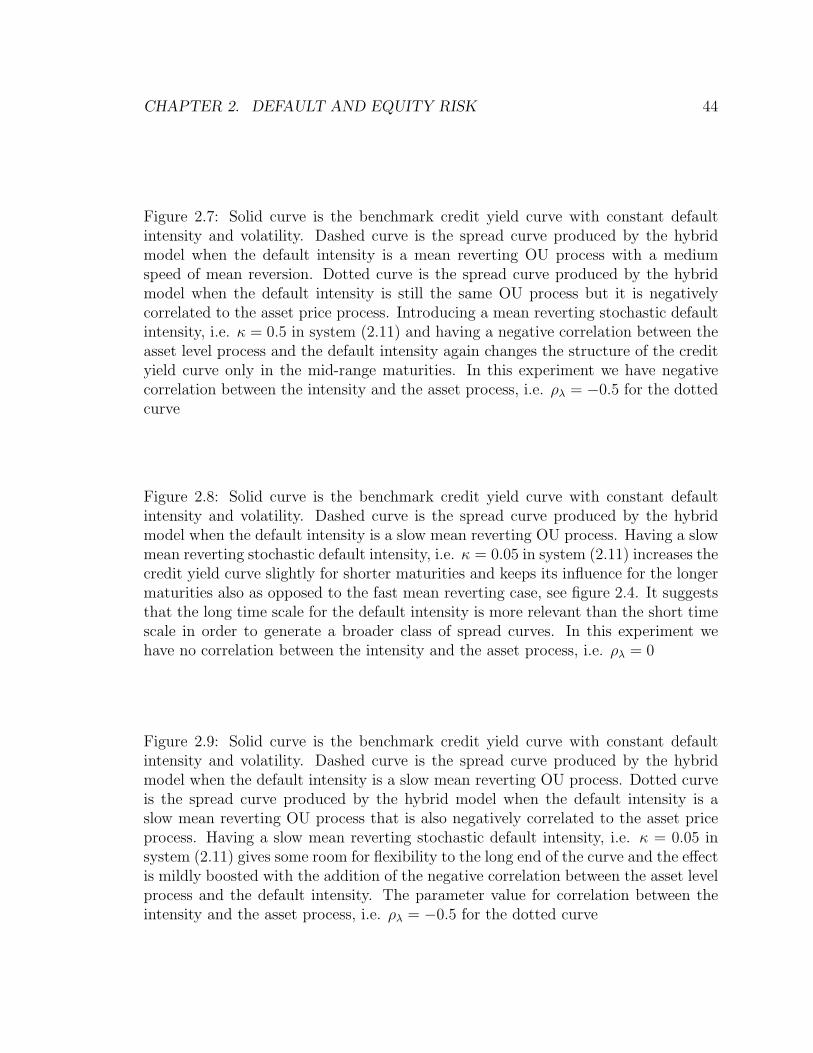
CHAPTER 2. DEFAULT AND EQUITY RISK 44
Figure 2.7: Solid curve is the benchmark credit yield curve with constant defaultintensity and volatility. Dashed curve is the spread curve produced by the hybridmodel when the default intensity is a mean reverting OU process with a mediumspeed of mean reversion. Dotted curve is the spread curve produced by the hybridmodel when the default intensity is still the same OU process but it is negativelycorrelated to the asset price process. Introducing a mean reverting stochastic defaultintensity, i.e. κ = 0.5 in system (2.11) and having a negative correlation between theasset level process and the default intensity again changes the structure of the credityield curve only in the mid-range maturities. In this experiment we have negativecorrelation between the intensity and the asset process, i.e. ρλ = −0.5 for the dottedcurve
Figure 2.8: Solid curve is the benchmark credit yield curve with constant defaultintensity and volatility. Dashed curve is the spread curve produced by the hybridmodel when the default intensity is a slow mean reverting OU process. Having a slowmean reverting stochastic default intensity, i.e. κ = 0.05 in system (2.11) increases thecredit yield curve slightly for shorter maturities and keeps its influence for the longermaturities also as opposed to the fast mean reverting case, see figure 2.4. It suggeststhat the long time scale for the default intensity is more relevant than the short timescale in order to generate a broader class of spread curves. In this experiment wehave no correlation between the intensity and the asset process, i.e. ρλ = 0
Figure 2.9: Solid curve is the benchmark credit yield curve with constant defaultintensity and volatility. Dashed curve is the spread curve produced by the hybridmodel when the default intensity is a slow mean reverting OU process. Dotted curveis the spread curve produced by the hybrid model when the default intensity is aslow mean reverting OU process that is also negatively correlated to the asset priceprocess. Having a slow mean reverting stochastic default intensity, i.e. κ = 0.05 insystem (2.11) gives some room for flexibility to the long end of the curve and the effectis mildly boosted with the addition of the negative correlation between the asset levelprocess and the default intensity. The parameter value for correlation between theintensity and the asset process, i.e. ρλ = −0.5 for the dotted curve

CHAPTER 2. DEFAULT AND EQUITY RISK 45
2.5 Modelling Default Risk
2.5.1 Merton’s Model with Surprise Defaults
Assuming the setting of system (2.11) for the asset price process and the intensity
process. In this section we define the structural component of the default as in
Merton’s case i.e. default happens if St is below the default boundary K at time T
and also we have a stochastic, mean reverting exogenous default intensity. Motivated
by the results of numerical experiments of the previous section 2.4, we choose a slowly
mean reverting one i.e. the system (2.11) looks likedSt = (r + λ∗t )Stdt+ σStdW
∗St
dXt = [δ(b−Xt)−√δΛ2]dt+
√δβλ
√2κdW ∗λ
t
λ∗t = φtg(Xt)
(2.12)
where δ is a small parameter. So the price of a defaultable zero-coupon bond in this
case would be (2.11).
P δ(t, s, x) = E∗e−(r+λ(x))(T−t)h(ST )|St = s,Xt = x (2.13)
where we denote the δ dependence as a super script and also we drop the ∗ notation
for λ for the rest of the section keeping in mind that we are already under the risk
neutral measure. As a particular case of the formula (2.5) we obtain∂P δ
∂t+ L(S,X)P
δ − (r + λ(x))P δ = 0
P δ(T, s, x) = h(s)(2.14)
where L(S,X) is the infinitesimal generator of the two dimensional Markovian Process
(St, Xt). Then we define the operator Lδ as follows
Lδ =∂
∂t+ L(S,X) − (r + λ(x))(·)

CHAPTER 2. DEFAULT AND EQUITY RISK 46
so that the system (2.14) becomes:LδP δ(t, s, x) = 0
P δ(T, s, x) = h(s)(2.15)
If we choose in particular h(s) = 1 then we are in the case of a defaultable bond.
In order to calculate the approximate solutions for P δ we decompose the operator Lδ
according to the powers of√δ as follows:
Lδ = L2 +√δM1 + δM2
L2 = ∂∂t
+ 12σ2s2 ∂2
∂s2+ (r + λ(x))(s ∂
∂s− ·)
M1 = βλ(ρλσs∂2
∂s∂x− Λ2
∂∂x
)
M2 = δ(b− x) ∂∂x
+ 12β2λ∂2
∂x2
(2.16)
We expand the P δ in powers of√δ
P δ = P0 +√δP1 + δP2 + · · ·
plugging this in equation (2.15) and using the operator notation introduced in (2.16)
we get
L2P0 +√δ(L2P1 +M1P0) + δ(L2P2 +M1P1 +M2P0) + · · · = 0
Hence, matching the first two terms and the terminal conditions we can define the
P0&P1 as a solution of the following two systems of equations:L2P0 = 0
P0(T, s, x) = h(s)
L2P1 +M1P0 = 0
P1(T, s, x) = 0(2.17)
Both P0&P1 depend on x as a parameter since the operators L2 = LBS(σ, r + λ(x))
do not take derivatives with respect to x variable. Hence, the leading term is the

CHAPTER 2. DEFAULT AND EQUITY RISK 47
solution of the system LBS(σ, r + λ(x))P0 = 0
P0(T, s, x) = h(s)
Note that P0 depends on x only through the adjusted default rate, so x is only a
parameter that defines P0. So the leading term P0 = PBS(σ, r + λ(x)) which is given
by equation (2.6). Next, we derive an expression for P1.
Proposition 1:
Let
M1 = V δ1 s
∂
∂s(∂
∂x) + V δ
0
∂
∂x(2.18)
The function P1(t, s, x) is explicitly given by
P1(t, s, x) = (T − t)(V δ1 s
∂
∂s(∂P0
∂x) + V δ
0
∂P0
∂x)− 1
2(T − t)2(
∂λ
∂x(s∂
∂s− ·)2P0) (2.19)
For a proof and the explicit form of the correction term see section AppendixD.
2.5.2 First Passage Model with Surprise Defaults
Now we change the problem slightly. We adopt the setting of the section 2.5.1 and
system (2.12). But we extend the definition of the structural component of the default
to any time the asset process St hits the default boundary level K until maturity,T ,
as opposed to just at time T . Therefore, the price of a defaultable zero-coupon bond
in this case would be
P δ(t, s, x) = Ee−(r+λ(x))(T−t)h(ST )1inft≤u≤T Su>K|St = s,Xt = x

CHAPTER 2. DEFAULT AND EQUITY RISK 48
The price function satisfies almost the same PDE system as in the Merton’s case
except for the additional boundary condition at the default barrier.∂P δ
∂t+ L(S,X)P
δ − (r + λ(x))P δ = 0
P δ(t,K, x) = 0
P δ(T, s, x) = h(s)
Using barrier options approach, we introduce the function u(t, s, x) as
P δ(t, s, x) = 1inf0≤u≤t Su>Ku(t, St = s,Xt = x)
where the function u(t,s,x) satisfies,for s ≥ K, the system∂u∂t
+ L(S,X)u− (r + λ(x))u = 0 on s > K, t < T
u(t,K, x) = 0 for t ≤ T
u(T, s, x) = h(s) for s > K
The equation solved by the first term of the asymptotic expansionLBS(σ, r + λ(x))u0 = 0 on s > K, t < T
u0(t,K, x) = 0 for t ≤ T
u0(T, s, x) = h(s) for s > K
for a frozen value of x. Equation solved by the first correction termLBS(σ, r + λ(x))u1 +M1u0 = 0 on s > K, t < T
u1(t,K) = 0 for t ≤ T
u1(T, s) = 0 for s > K
(2.20)
The closed-form solution of the system (2.20) is given in Appendix D. In consequence,
we approximate the price of a defaultable zero-coupon bond
P δ(0.T ) ∼ u0(0, s) +√δu1(0, s)

CHAPTER 2. DEFAULT AND EQUITY RISK 49
Figure 2.10: Solid curve is the spreads produced by the simple hybrid model withconstant default intensity and the volatility. Dashed curve is the spreads produced bythe model where the default intensity process is a mean reverting stochastic processusing the approximate solution derived in section 2.5.2. Qualitatively, the correctionto the spreads does not have much short run effect but has a persistent change in thelong run as expected from the simulated results. Quantitatively, although approxi-mate formula goes only up to the first order, it still fits the simulated data points witha small least squares error with the calibration of very few parameters. Parametervalues are V δ
0 = 0.002, V δ1 = −0.008, λ∗ = 0.01, σ∗ = 0.12 and s
K= 1.3
Resulting spreads from the approximate formula with the fitted parameters are com-
pared to the spreads obtained from the hybrid model with constant intensity in figure
2.10. The difference between the two curves is due to the stochasticity of the default
intensity. As expected from the slowly mean reverting choice for the default inten-
sity, the spreads are almost the same in the short term but rather different for longer
maturities.

CHAPTER 2. DEFAULT AND EQUITY RISK 50
2.6 Stochastic Volatility with Fast Mean Rever-
sion
In the context of equity markets and derivatives pricing and hedging, stochastic
volatility is recognized as an essential feature in the modelling of the underlying dy-
namics. For an extended discussion we refer to Willmott et al.[69] and the references
in there. In order to illustrate our approach we consider first the case where volatility
is driven by one factor which we assume to be a mean-reverting Gaussian diffusion,
i.e. an Ornstein-Uhlenbeck process. The dynamics under the physical measure is
described by the following pair of SDEs
dSt = µStdt+ σ(Yt)StdWSt
dYt = α(m− Yt)dt+ ν√
2αdW Yt
with a constant exogenous default intensity λ. Main assumptions of our framework
are
i. The volatility function σ is positive, non-decreasing and bounded away and
above from 0.
ii. The invariant distribution of the volatility factor Y is the Gaussian distribution
with mean m and standard deviation ν and it is independent of the parameter
α.
iii. The important parameter α > 0 is the rate of mean reversion of the process Y
. In other words 1/α is the time scale of this process, meaning that it reverts
to its mean over times of order 1/α. Small values of α correspond to slow mean
reversion and large values of α correspond to fast mean reversion.
Also, the standard Brownian motions W S and W Y are correlated as
EdW St dW
Yt = ρσdt

CHAPTER 2. DEFAULT AND EQUITY RISK 51
where ρσ is a constant correlation coefficient satisfying ρσ < 1. We remark that
for the purpose of illustration we choose the volatility factor to be an Ornstein-
Uhlenbeck process, however, in our approach, Y could be any ergodic diffusion with
a unique invariant distribution, as explained in more detail in Fouque et al (2000)[27].
Moreover, in our simulations we choose particular volatility functions σ(y) as being
proportional to max(c1,min(c2, exp(y))), that is the exponential function with lower
and upper cutoffs.
In order to price defaultable bonds under this model for the underlying we rewrite it
under a risk neutral measure using previous section’s results, chosen by the market
through the market price of volatility risk Λ1 and default risk of φ, as followsdSt = (r + λ∗)Stdt+ σ(Yt)StdW
∗St
dYt = (α(m− Yt)− ν√
2αΛ1(Yt))dt+ ν√
2αdW ∗Yt
(2.21)
with an exogenous default intensity λ∗ = φλ. Here, W ∗St and W ∗Y
t are standard
Brownian motions under the risk-neutral measure and correlated under the physical
measure. We assume that the market price of volatility risk Λ1 is bounded and a
function of y only whereas φ is just a constant.
In this section, we compute the yield spreads that results when we use the stochastic
volatility model in (2.21). Our focus is the combined role of the mean reversion time1α
and the correlation ρσ on the yield spread curve. We use various values for α,
corresponding to volatility factors that range from slowly mean reverting α = .05 to
fast mean reverting α = 10. For each value of α we present the uncorrelated case
ρσ = 0 and a negatively correlated case which is ρσ = −0.5. In each figure we plot the
yield spread curves as functions of time to maturity, and the solid curve corresponds
to a constant volatility. The dashed curve is the yield curve under the stochastic
volatility model (2.21), where the initial volatility level σ(Y0) and the long-run av-
erage volatility (see (2.22) below) coincide with the volatility level for the constant
volatility case. The constant volatility yields are computed using the explicit formula
(2.10). The stochastic volatility yields are computed using Monte Carlo simulations
of trajectories for the model (2.21). For these illustrations we choose the following
parameter values: Λ1 = 0, sK
= 1.2, σ(Y0) = 0.12, r = 0.06,m = 0.12, ν = 0.6.

CHAPTER 2. DEFAULT AND EQUITY RISK 52
Figure 2.11 illustrates the effects of a slowly mean reverting volatility with no correla-
tion between the volatility and the underlying processes and 2.12 is the same setting
with negative correlation which is almost the same. The yields for short maturities
are not significantly affected. There is a mild spread increase for longer maturities
and this increase is slightly lower with zero correlation. This feature of the curve was
already captured with the setting of section 2.5.2.
Figure 2.13 illustrates the effects of stochastic volatility that runs on a medium time
scale. We observe that the effect is similar to an increase in volatility as shown in
Figure 2.3. This effect is again enhanced by negative correlation as seen in figure
2.14. This feature of the curve will be captured in the leading order term by choosing
an appropriate effective volatility level σ∗ as explained in section 2.7.3.
Figure 2.15 illustrates the effects of a fast mean reverting volatility, without and and
figure 2.16 with negative correlation. In this case the yields for short maturities are
significantly affected and the effect is enhanced by the presence of a small negative
correlation. It is remarkable that this effect is qualitatively and quantitatively very
different from the effect resulting from an increase in the volatility level as shown in
figure 2.3. This feature of the curve will be captured in our analysis of the stochastic
volatility model with a fast mean reverting volatility factor in the following section
2.7.3. We conclude from these numerical experiments that the time scale content of
stochastic volatility is crucial in the shaping of the yield spread curve. In particular,
a short time scale with a negative correlation gives enhanced spreads at short matu-
rities, as compared with the constant volatility case.
A well separated fast volatility time scale has been observed in equity [30] and fixed
income [11] markets. A main feature of this short time scale is that it can be treated
by singular perturbation techniques as described in detail in [29]. This leads to a
description where the effects of the stochastic volatility can be summarized in terms
of three group market parameters, an effective constant volatility σ∗, leverage sK
and
a skew parameter V ε3 . Below we will generalize these results to the case of defaultable
bonds.

CHAPTER 2. DEFAULT AND EQUITY RISK 53
Figure 2.11: Solid curve is the benchmark credit yield curve with constant defaultintensity and volatility. Dashed curve is the spread curve produced by the hybridmodel when the volatility of the underlying asset level process is a slow mean revertingOU process. Introducing a slow mean reverting stochastic volatility, i.e. α = 0.05 insystem (2.21) increases the credit yield curve slightly for shorter maturities but liftsit up more for longer maturities. In this experiment we have no correlation betweenthe volatility and the asset level process, i.e. ρσ = 0. We also take Λ1 = 0 so there isno risk premium due to volatility risk
Figure 2.12: Solid curve is the benchmark credit yield curve with constant defaultintensity and volatility. Dashed curve is the spread curve produced by the hybridmodel when the the volatility of the underlying asset level process is an OU processwith slow mean reversion. Dotted curve is the spread curve produced by the hybridmodel when the volatility is a slow mean reverting OU process that is also negativelycorrelated to the asset price process. Introducing a slow mean reverting stochasticvolatility, i.e. α = 0.05 in system (2.21) also having a negative correlation betweenthe asset level process and the volatility pushed the spread curve further up for longermaturities as expected while keeping the short term structure unchanged from theno correlation case. In this experiment we have negative correlation between thevolatility and the asset process, i.e. ρσ = −0.5 for the dotted curve.
2.7 Modelling Equity Risk
2.7.1 Merton’s Model with Stochastic Volatility
We first review the singular perturbation results in the case of a European option.
Let the payoff function at the maturity time T be h(s). The price of the option is
obtained as the expected value of the discounted payoff under the risk neutral measure
in the stochastic volatility model (2.21):
P ε(t, s, y) = Ee−(r+λ∗)(T−t)h(ST )|St = s, Yt = y
In Fouque et al. (2000)[27] it is shown that in the limit of the volatility time scale
going to zero, or equivalently alpha goes to infinity, the price P ε converges to the

CHAPTER 2. DEFAULT AND EQUITY RISK 54
Figure 2.13: Solid curve is the benchmark credit yield curve with constant defaultintensity and volatility. Dashed curve is the spread curve produced by the hybridmodel when the volatility of the underlying asset level process is a mean revertingOU process where the level mean reversion speed is medium, i.e. α = 0.5 in system(2.21). The shift in the overall shape is spread out and the lift is larger than the slowmean reverting volatility case which gives more variety overall. In this experimentwe have no correlation between the volatility and the asset level process, i.e. ρσ = 0.
Figure 2.14: Solid curve is the benchmark credit yield curve with constant defaultintensity and volatility. Dashed curve is the spread curve produced by the hybridmodel when the the volatility of the underlying asset level process is a mean revertingOU process where the level of mean reversion is medium, i.e. α = 0.5 in system(2.21). Having mean reversion in the volatility process combined with the effect ofthe correlation with the asset level process yields more flexibility to the spread curvefor mid-range maturities while not changing too many things about the short or longterm structure from the no correlation case. In this experiment we have negativecorrelation between the volatility and the asset process, i.e. ρσ = −0.5 which resultedthe dotted curve.
Figure 2.15: Solid curve is the benchmark credit yield curve with constant default in-tensity and volatility. Dashed curve is the spread curve produced by the hybrid modelwhen the volatility of the underlying asset level process is a a fast mean reverting OUprocess, i.e. α = 10 in system (2.21). The short term spreads increase much morerapidly allowing for sudden changes in short period of times. Although the idea ofhaving the hybrid model approach takes care of non-zero initial yield spreads, intro-duction of fast mean reverting stochastic volatility help generating quckly changingterm structures. The setting is not any different than the constant case for longermaturities. In this experiment we have no correlation between the volatility and theasset level process, i.e. ρσ = 0.

CHAPTER 2. DEFAULT AND EQUITY RISK 55
Figure 2.16: Solid curve is the benchmark credit yield curve with constant defaultintensity and volatility. Dashed curve is the spread curve produced by the hybridmodel when the the volatility of the underlying asset level process is a mean revertingOU process where the level of mean reversion is fast, i.e. α = 10 in system (2.21).Having fast mean reversion in the volatility process combined with the effect of thecorrelation with the asset level process yields more dramatic changes to the short endof the spread curve but still converges to the constant volatility case as the maturitiesget larger. In this experiment we have negative correlation between the volatility andthe asset process, i.e. ρσ = −0.5 which pushed up the dashed and resulted the dottedcurve.
Black-Scholes price computed with an effective constant volatility σ given by
σ2 =< σ2(·) >=1√2πν
∫σ2(y)e−
(y−m)2
2ν2 dy (2.22)
where σ2 is averaged with respect to the invariant distribution of the OU process.
This limiting price, denoted by PBS(t, s) satisfies the following system
LBS(σ, r + λ∗)PBS = 0
PBS(T, s) = h(s)
where LBS(σ, r + λ∗) is given by
LBS(σ, r + λ∗) =∂
∂t+
1
2σ2s2 ∂
2
∂s2+ (r + λ∗)(s
∂
∂s− ·)
The main effects of stochastic volatility are captured by the first order correction
proportional to 1/α = ε and denoted by P 1(t, s). It is given as the solution of the
problem LBS(σ, r + λ∗)P 1 = −V ε
2 s2 ∂2PBS
∂s2− V ε
3 s∂∂s
(s2 ∂2PBS
∂s2)
P 1(T, s) = 0

CHAPTER 2. DEFAULT AND EQUITY RISK 56
where the parameters V ε2 and V ε
3 are small of order ε, and are complicated functions
of the original model parameters. Note that the first order price approximation
P ε(t, s, y) ∼ PBS(t, s) + P 1(t, s)
does not depend on the current level y of the volatility factor which is not directly
observed. The calibration is simplified by introducing the corrected effective volatility:
σ∗2 = σ2 + 2V ε2 (2.23)
and the BS price P∗BS computed at the volatility level σ∗. We define the correction
term P∗1 by
LBS(σ∗, r + λ∗)P∗1 = −V3s
∂∂s
(s2 ∂2P
∗BS
∂s2)
P∗1(T, s) = 0
so that
P (t, s, y) ∼ P∗BS(t, s) + P
∗1(t, s)
The accuracy of this approximation is of order 1α
in the case of a smooth payoff h,
and of order logαα
in the case of call options as proved in Fouque et al (2003)[31].
Observe that σ∗,λ∗ and V ε3 are the only parameters needed to compute this approxi-
mation, in fact, they can be calibrated from implied volatilities as explained in Fouque
(2004)[34].
2.7.2 First Passage Model with Stochastic Volatility
Here we consider an option that pays h(ST ) at maturity time T if the the underlying
stays above a level K before time T and zero otherwise. Under the model (2.21) for
the underlying, the price at time zero of this down and out barrier option is given by
P ε(0, s, y) = e−(r+λ∗)TE∗h(ST )1inf0≤u≤T Su>K|S0 = s, Y0 = y

CHAPTER 2. DEFAULT AND EQUITY RISK 57
We define u(t, s, y) by
u(t, s, y) = e−(r+λ∗)(T−t)E∗h(ST )1inft≤u≤T Su>K|St = s, Yt = y
so that the price of the barrier option at time t is given by
P ε(t) = 1inf0≤u≤0 Su>Ku(t, St, Yt)
The function u(t, s, y) satisfies for s ≥ K the problem( ∂∂t
+ LS,Y − (r + λ∗))u = 0 on s > K, t < T
u(t,K) = 0 for t ≤ T
u(T, s) = h(s) for s > K
where LS,Y is the infinitesimal generator of the two dimensional process (S, Y ) given
by (2.21).
Following Fouque et al (2000)[27], in the limit as ε approaches zero we find that
u(t, s, y) converges to u0(t, s) which solves the constant volatility problemLBS(σ, r + λ∗)u0 = 0 on s > K, t < T
u0(t,K) = 0 for t ≤ T
u0(T, s) = h(s) for s > K
As in the European case, for calibration purposes, it is convenient to use the adjusted
effective volatility σ∗ defined in (2.23). Hence, we define u∗0(t, s) as the solution of
the problem LBS(σ∗, r + λ∗)u∗0 = 0 on s > K, t < T
u∗0(t,K) = 0 for t ≤ T
u∗0(T, s) = h(s) for s > K
(2.24)

CHAPTER 2. DEFAULT AND EQUITY RISK 58
and we define the correction u∗1(t, s) byLBS(σ∗, r + λ∗)u∗1 = −V ε
3 s∂∂s
(s2 ∂2u∗0∂s2
) on s > K, t < T
u∗1(t,K) = 0 for t ≤ T
u∗1(T, s) = 0 for s > K
(2.25)
Note that, the small parameter V ε3 is the same as in the European case.
2.7.3 Pricing Formulas and Implied Spreads
In this section we consider the case h(s) = 1 corresponding to a defaultable zero-
coupon bond. From formula (2.6) (2.25) in section 2.7.2 we find that u∗0 defined in
(2.24) is explicitly given by
u∗0(t, s) = e−(r+λ∗)(T−t)(N(d+)− (s
K)pN(d−)) (2.26)
with the notation
p = 1− 2(r + λ∗)
σ∗2, d± =
± log( sK
)− pσ∗2
2τ
σ∗√τ
where we dropped the ∗ and τ inside d± for notational simplicity. As a result of all,
the price of the defaultable bond at time 0 is approximated by
P (0.T ) ∼ u∗0(0, s) +√εu∗1(0, s)
where u∗0(t, s) is given in equation (2.26) and u∗1(t, s) = y1(t, s) + y2(t, s) which are
derived in Appendix E. Here we state the final answer.
y1(t, s) = (T − t)V ε3 e
−(r+λ(x))(T−t)[N ′(d+)[d2+−1
(σ∗√τ)3
+ d+(σ∗
√τ)2
]
+ N ′(d−)[d2−−1
(σ∗√τ)3
+ (3p−1)d−(σ∗
√τ)2
+ p(3p−2)(σ∗
√τ)
]( sK
)p
+ N(d−)[(1− p)p2]( sK
)p]

CHAPTER 2. DEFAULT AND EQUITY RISK 59
Figure 2.17: Solid curve is the spreads produced by the simple hybrid model withconstant default intensity and the volatility. Dotted curve is the spreads produced bythe model where the default intensity process is a mean reverting stochastic processusing the approximate solution derived in section 2.7.3. Qualitatively, the correctionto the spreads does not have much long run effect as we observed numerical experi-ments the fast mean reverting stochastic volatility converges to the constant volatilitycase as the maturity gets large but has a dramatic effect to the short end of the curve.Quantitatively, although approximate formula goes only up to the first order, it stillfits the simulated data points with a small least squares error with the calibrationof very few parameters. Used parameter values are V ε
3 = −0.003 and σ∗ = 0.12 andsK
= 1.2
and
y2(t, s) =( sK
)p/2
σ∗√
2π
∫ T
t
log sK
(z − t)3/2e−
log( sK
)2
2σ∗2(z−t) e((σ∗p)2
8+r+λ∗)(z−t)g(z)dz

CHAPTER 2. DEFAULT AND EQUITY RISK 60
Figure 2.18: Solid curve is the spreads produced by the simple hybrid model withconstant default intensity and the volatility. Dotted curve is the spreads produced bythe model where the stochastic volatility process is a mean reverting one using witha speed of mean reversion parameter α = 10. Qualitatively, the correction to thespreads does not have much long run effect and converges to the constant volatilitycase as the maturity gets large but has a dramatic effect to the short end of the curve.Dotted curve is the exact same setting with an even faster mean reverting processwhere α = 20. although the short term yields increase a little more, the long runbehavior is still the same. Existence of a long time scale is important in having longterm flexibility for credit yield spreads.
2.8 Modelling Default and Equity Risk:
2.8.1 Combined Framework and Mathematical Derivations
Just like the previous section’s approach, we start from the case of pricing of a Eu-
ropean derivative this time under the setting of (2.5) where we have both stochastic
volatility and the intensity at the same time. Therefore we have the slow and fast
time scales together, we will carry out a two dimensional version of the asymptotic
analysis done in sections 2.5 and 2.7. As a result of the analysis we will have two
correction terms, one due to short scale and another one due to long. And they would
separately represent the additional default risk for the stochastic intensity and the
addition equity risk for the stochastic volatility.
Before we move on to the mathematical analysis part, we run simulations to test
the flexibility of each factor and the interaction between the two factors. As seen in
figure 2.18, no matter how big the speed of mean reversion for the volatility factor it
always converges to a constant volatility model in the long run. Although it pushed
the short term spreads upwards, has almost no long term effect.
On the other hand as figure 2.19 suggests, the slow mean reversion factor takes over
in the long run and provides some freedom to the long end of the spread curve with-
out changing it much in the short end. And the effect is boosted by the negative
correlation parameter as in figure 2.20 We start with computing

CHAPTER 2. DEFAULT AND EQUITY RISK 61
Figure 2.19: Solid curve is the spreads produced by the simple hybrid model withconstant default intensity and the volatility. Dotted curve is the spreads produced bythe model where the stochastic volatility process is a mean reverting one using with aspeed of mean reversion parameter α = 10. Dotted curve is the hybrid model wherewe also a stochastic default intensity. A slow mean reverting process is used,κ = 0.1and we observe the effect of the addition to the long end of the curve without changingtoo much the short end of the curve.
Figure 2.20: Solid curve is the spreads produced by the simple hybrid model withconstant default intensity and the volatility. Dashed curve is the hybrid model wherewe have a fast mean reverting stochastic volatility and slow mean reverting defaultintensity, that is α = 10 and κ = 0.1 in (2.5). We further boost the effect of thestochastic default intensity with the introduction of a negative correlation of 50%with the underlying state process. It effects the curve overall both in the long runand short run. The combination of the time scales and the correlation parametersyields a broad set of credit yield spreads with realistic features. Parameter value forcorrelation is ρλ = −0.5
P ε,δ(t, St, Yt, Xt) = E∗e−(r+λ∗)(T−t)h(ST )|St, Yt, Xt (2.27)∂P ε,δ
∂t+ L(S,Y,X)P
ε,δ − (r + λ∗)P ε,δ = 0
P ε,δ(T, s, y, x) = h(s)(2.28)
where L(S,Y,X) is the infinitesimal generator of the Markovian Process (St, Yt, Xt).
Then we define the operator Lε,δ as follows
Lε,δ =∂
∂t+ L(S,Y,X) − (r + λ(x))(·)
so that the system (2.28) becomes:Lε,δP ε,δ = 0
P ε,δ(T, s, y, x) = h(s)(2.29)

CHAPTER 2. DEFAULT AND EQUITY RISK 62
If we choose in particular h(s) = 1 then we are in the case of defaultable bond.
In order to calculate the approximate solutions for P ε,δ we decompose the operator
Lε,δ according to the powers of√ε and
√δ as follows:
Lε,δ = 1εL0 + 1√
εL1 + L2 +
√δM1 + δM2 +
√δεM3
L0 = (m− y) ∂∂y
+ 12β2σ∂2
∂y2
L1 = βσ(ρσσ(y)s ∂2
∂s∂y− Λ1(y, x)
∂∂y
)
L2 = ∂∂t
+ 12σ2(y)s2 ∂2
∂s2+ (r + λ(x))(s ∂
∂s− ·)
M1 = βλ(ρλσ(y)s ∂2
∂s∂x− Λ2(y, x)
∂∂x
)
M2 = δ(b− x) ∂∂x
+ 12β2λ∂2
∂x2
M3 = βσρσρλβλ∂2
∂y∂x
(2.30)
We expand the P ε,δ in powers of√δ first
P ε,δ = P ε0 +
√δP ε
1 + δP ε2 + · · ·
plugging this in equation (2.29) and using the operator notation introduced in (2.30)
we get
(1
εL0+
1√εL1+L2)P
ε0+√δ(1
εL0+
1√εL1+L2)P
ε1+(M1+
1√εM3)P
ε0+· · · = 0 (2.31)
Hence, matching the first two terms and the terminal conditions we can define the
P ε0&P
ε1 as a solution of the following two systems of equations:
(1εL0 + 1√
εL1 + L2)P
ε0 = 0
P ε0(T, s, y, x) = h(s)
(1εL0 + 1√
εL1 + L2)P
ε1 + (M1 + 1√
εM3)P
ε0 = 0
P ε1(T, s, y, x) = 0

CHAPTER 2. DEFAULT AND EQUITY RISK 63
Both P ε0&P
ε1 depend on x as a parameter since the operators L0,L1,L2 do not take
derivatives with respect to x. Consider the first term P ε0 and expand it as
P ε0 = P0 +
√εP1,0 + εP2,0 + ε3/2P3,0 + · · · (2.32)
In the notation Pi,j i corresponds to power of√ε and j corresponds to the power of
√δ. Our ultimate goal in this section would be calculating the approximate formula
P ε,δ ≈ P0 +√εP1,0 +
√δP0,1
Inserting (2.32) in (2.31) we get
1εL0P0 + 1√
ε(L0P1,0 + L1P0)
+(L0P2,0 + L1P1,0 + L2P0)
+√ε(L0P3,0 + L1P2,0 + L2P1,0)
+ · · · = 0
(2.33)
Matching the first term and using (2.30) we get
L0P0 = (α(m− y)∂
∂y+
1
2β2σ
∂2
∂y2)P0 = 0
Here we choose P0 to be independent of y so that we do not get any unreasonable
growth, i.e. P0 = P0(t, s, x)). Also matching the second term gives us
L0P1,0 + L1P0 = 0 (2.34)
But since the operator L1 takes derivatives with respect to y and P0 is constant in y
L1P0 = 0 and the equation (2.34) reduces to
L0P1,0 = 0

CHAPTER 2. DEFAULT AND EQUITY RISK 64
Now, we also choose P1,0 not to depend on y, i.e. P1,0 = P1,0(t, s, x)). Then, order 1
terms in (2.33) gives
L0P2,0 + L2P0 = 0 (2.35)
Notice that (2.35) is a Poisson equation in P2,0 with respect to y variable. So only
reasonable solution occurs in case of L2P0 being in the orthogonal complement of L∗0.
Namely,
< L2P0 >= 0 (2.36)
where the <> denotes the integration with respect to the invariant distribution Φ of
the process Yt. Since, P0 does not depend on y < L2P0 >=< L2 > P0 and
< L2 >=∂
∂t+
1
2< σ2(·) > s2 ∂
2
∂s2+ (r + λ(x))(s
∂
∂s− .)
which is the LBS(σ, r + λ(x)) where σ is the effective volatility and r + λ(x) is the
default adjusted short rate.
σ2 =< σ2(·) >=
∫σ2(y)Φ(dy)
Hence, the leading term is the solution of the systemLBS(σ, r + λ(x))P0 = 0
P0(T, s, x) = h(s)(2.37)
Note that P0 depends on x only through the adjusted default rate, so x is only a
parameter that defines P0 Next, we derive an expression for P1,0.√ε term in (2.33)
gives
L0P3,0 + L1P2,0 + L2P1,0 = 0
Then, the same averaging condition gives
< L1P2,0 > + < L2 > P1,0 = 0

CHAPTER 2. DEFAULT AND EQUITY RISK 65
Then, (2.35) and (2.36) gives
P2,0 = −L−10 (L2− < L2 >)P0
Introduce the notation
A = − < L1L−10 (L2− < L2 >) > (2.38)
Then, we can define the P1,0 as the solution of the system of systemLBS(σ, r + λ∗(x))P1,0 +AP0 = 0
P1,0(T, s, x) = 0
Observe that, P1,0 is the solution of a Black-Scholes equation with a source term and
zero terminal condition.
Computation of the operator A:
Let ψ(y) be the solution of the Poisson Equation with respect to y
L0ψ(y) = σ2(y)− σ2
then
L−10 (L2− < L2 >) =
1
2ψ(y)s2 ∂
2
∂s2
and therefore
L1L−10 (L2− < L2 >) = βσ(ρσσ(y)s ∂2
∂s∂y− Λ1(y, x)
∂∂y
)12ψ(y)s2 ∂2
∂s2(2.39)
= ρσβσσ(y)2
∂ψ∂ys ∂∂s
(s2 ∂2
∂s2)− βσΛ1(y,x)
2∂ψ∂ys2 ∂2
∂s2

CHAPTER 2. DEFAULT AND EQUITY RISK 66
By averaging in y with respect to the invariant distribution and using (2.38) of the
operator A we get
A = 12< βσΛ1(y, x)
∂ψ∂y> s2 ∂2
∂s2− ρσ
2< βσσ(y)∂ψ
∂y> s ∂
∂ss2 ∂2
∂s2(2.40)
≡ V ε3 s
2 ∂2
∂s2− V ε
2 s∂∂ss2 ∂2
∂s2(2.41)
where the bracketed terms are functions of x
Proposition 1:
The function P1,0(t, s, x) is explicitly given by
P1,0 = (T − t)AP0
where the operator A is as in equation (2.38) and P0 as in equation (2.37).
Consider the term P ε1 and expand it as
P ε1 = P0,1 +
√εP1,1 + εP2,1 + ε3/2P3,1 + ... (2.42)
Inserting (2.42) in (2.33) we get
1εL0P0,1 + 1√
ε(L0P1,1 + L1P0,1 +M3P0)
+(L0P2,1 + L1P1,1 + L2P0,1) +M1P0 +M3P1,0
+√ε(L0P3,1 + L1P2,1 + L2P1,1 +M1P1,0 +M3P2,0)
+ · · · = 0
(2.43)
Matching the first term and using (2.30) we get
L0P0,1 = (α(m− y)∂
∂y+
1
2β2σ
∂2
∂y2)P0,1 = 0
Here we choose P0,1 to be independent of y just like for P0. Also matching the second
term gives us
L0P1,1 + L1P0,1 +M3P0 = 0 (2.44)

CHAPTER 2. DEFAULT AND EQUITY RISK 67
But since the operator L1 takes derivatives with respect to y and P0,1 is constant in y
L1P0,1 = 0. Similarly, M3 takes derivative with respect to y and P0 does not depend
on y. Hence, the equation (2.44) reduces to
L0P1,1 = 0
Now, we also choose P1,1 not to depend on y, i.e. P1,1 = P1,1(t, s, x)). Then, order 1
terms in (2.43), using the facts L1P1,1 = M3P1,0 gives us
L0P2,1 + L2P0,1 +M1P0 = 0 (2.45)
Notice that (2.45) is a Poisson equation in P2,1 with respect to y variable. Then, the
averaging condition in this case turns out to be
< L2P0,1 +M1P0 >=< L2 > P0,1+ <M1 > P0 = 0
where <M1 > is
<M1 > = ρλ < βλ(·)σ(·) > s ∂2
∂s∂x− < βλ(·)Λ2(·, x) > ∂
∂x(2.46)
≡ V δ0 s
∂2
∂s∂x− V δ
1∂∂x
(2.47)
since the terminal condition h(x) is taken care of by the P0 term, we can write the
P0,1 as a solution to the systemLBS(σ, r + λ(x))P0,1+ <M1 > P0 = 0
P0,1(T, s, x) = 0
In fact, we can explicitly calculate the term P0,1 as in the following proposition. See
Appendix D for the actual derivation.

CHAPTER 2. DEFAULT AND EQUITY RISK 68
Proposition 2:
The function P0,1(t, s, x) is explicitly given by
P0,1 = (T − t) <M1 > P0 −1
2(T − t)2(
∂λ
∂x(s∂
∂s− ·)2P0) (2.48)
We start writing the first order approximation again by using the propositions of the
previous section
P ε,δ ≈ P0 +√εP1,0 +
√δP0,1
= P0 + (T − t)(√εA+
√δ <M1 >)P0 − 1
2(T − t)2(∂λ
∂x(s ∂
∂s− ·)2P0)
2.8.2 Risk due to Equity Risk
The short time scale contribution to P ε,δ is (T − t)√εAP0 so we consider the operator
√εA =
√ε
2< βσΛ1(·, x)
∂ψ
∂y> s2 ∂
2
∂s2)− ρσ
√ε
2< βσσ(·)∂ψ
∂y> s
∂
∂ss2 ∂
2
∂s2)
Then, we introduce the following notation for two parametersV ε
2 =√ε
2< βσΛ1(·, x)∂ψ∂y >
V ε3 = −ρσ
√ε
2< βσσ(·)∂ψ
∂y>
(2.49)
Now, we can rewrite the short time scale contribution to P ε,δ as
(T − t)√εAP0 = (T − t)(V ε
2 s2 ∂
2
∂s2) + V ε
3 s∂
∂ss2 ∂
2
∂s2))P0 (2.50)
2.8.3 Risk due to Default Risk
The long time scale contribution to P ε,δ is (T − t)√ε <M1 > P0− 1
2(T − t)2(∂λ
∂x(s ∂
∂s−
·)2P0) so we consider the operator
√δ <M1 >= [
ρλ√δ
2< βλσ(·) >]s
∂
∂s(∂
∂x) + [−
√δ
2< βλΛ2(·, x) >]
∂
∂x(2.51)

CHAPTER 2. DEFAULT AND EQUITY RISK 69
Then, we introduce the following notation for two parametersV δ
0 = −√δ
2< βλΛ2(·, x) >
V δ1 = ρλ
√δ
2< βλσ(·) >
Now, we can rewrite the long time scale contribution to P ε,δ as
(T − t)√ε <M1 > P0 = (T − t)(V δ
1 s∂
∂s(∂
∂x) + V δ
0
∂
∂x)P0 (2.52)
In summary, for the European case we calculate the default risk contribution as follows
(T − t)√ε <M1 > P0 −
1
2(T − t)2(
∂λ
∂x(s∂
∂s− ·)2P0)
where the three terms on RHS are respectively given by the equations (2.51) and
(D.10).
2.8.4 Bond Price and Yield Approximations
Again, we go to the case of pricing of the defaultable zero coupon bond where the
default could occur any time until the maturity. This time we simply write out the
final equations as we derived them separately in sections 2.5 and 2.7. Objective is
the compute the expectation
P ε,δ(t, St, Yt, Xt) = E∗e−(r+λ∗)(T−t)h(ST )1inft≤u≤T Su>K |St, Yt, Xt
We introduce the new function u(t, s, y, x)
P (t) = 1inf0≤u≤t Su>Ku(t, St, Yt, Xt)

CHAPTER 2. DEFAULT AND EQUITY RISK 70
where the function it satisfies,for s ≥ K, the system∂u∂t
+ L(S,Y,X)u− (r + λ(x))u = 0 on s > K, t < T
u(t,K) = 0 for t ≤ T
u(T, s) = h(s) for s > K
The equation solved by the first term of the asymptotic expansionLBS(σ, r + λ(x))u0 = 0 on s > K, t < T
u0(t,K) = 0 for t ≤ T
u0(T, s) = h(s) for s > K
for a frozen value of x. Equation solved by the first correction term from the short
time scale contributionLBS(σ, r + λ(x))u1,0 +Au0 = 0 on s > K, t < T
u1,0(t,K) = 0 for t ≤ T
u1,0(T, s) = 0 for s > K
(2.53)
Introducing the u∗1,0 = u1,0 + (T − t)Au0 the system becomesLBS(σ, r + λ(x))u∗1,0 = 0 on s > K, t < T
u∗1,0(t,K) = m(t) for t ≤ T
u∗1,0(T, s) = 0 for s > K
(2.54)
where m(t) = lims↓K(T − t)Au0 Equation solved by the first correction term from the
long time scale contributionLBS(σ, r + λ∗(x))u0,1+ <M1 > u0 = 0 on s > K, t < T
u0,1(t,K) = 0 for t ≤ T
u0,1(T, s) = 0 for s > K
(2.55)
CHAPTER 2. DEFAULT AND EQUITY RISK 71
Solution of the system (2.55) is a bit more involved than the (2.53) which we do in
Appendix D, but at the end it boils down to solving a similar homogeneous systemLBS(σ, r + λ(x))u∗0,1 = 0 on s > K, t < T
u∗0,1(t,K) = n(t) for t ≤ T
u∗0,1(T, s) = 0 for s > K
(2.56)
for some function n(t) defined in (D.18). In consequence, we approximate the price
of a defaultable zero-coupon bond
P (0.T ) ∼ u0(0, s) + u∗1,0(0, s)− (T − t)Au0(0, s)
+ u∗0,1(0, s)− (T − t) <M1 > u0(0, s)
+ 12(T − t)2(∂λ
∂x(s ∂
∂s− ·)2P0)
The integral formulas
u∗1,0(t, s) =( sK
)p/2
σ∗√
2π
∫ T
t
log sK
(z − t)3/2e−
log( sK
)2
2σ∗2(z−t) e((σ∗p)2
8+r+λ∗)(z−t)m(z)dz (2.57)
and
u∗0,1(t, s) =( sK
)p/2
σ∗√
2π
∫ T
t
log sK
(z − t)3/2e−
log( sK
)2
2σ∗2(z−t) e((σ∗p)2
8+r+λ∗)(z−t)n(z)dz (2.58)
along with the functions m(t) and n(t) are calculated explicitly in Appendix D.

CHAPTER 2. DEFAULT AND EQUITY RISK 72
Figure 2.21: Solid curve is the spreads produced by the simple hybrid model withconstant default intensity and the volatility. Dotted curve is the spreads producedby the model where both the default intensity and the stochastic volatility are meanreverting stochastic processes with slow and fast mean reversions respectively usingthe approximate solution derived in section 2.8.4. Qualitatively, the correction tothe spreads both have short term and long term effects. We have the non-zero shortterm spreads due to default intensity, quick changes in the short run due to fast meanreverting stochastic volatility and the necessary flexibility over the long run due toslow fast mean reverting stochastic intensity. And quantitatively, all the pricing andparameter fitting are done through approximate formula which goes only up to thefirst order and it still fits the simulated data points with a small least squares errorwith the calibration of the few parameters. The parameters obtained for the dottedcurve V ε
3 = −0.003,V δ0 = 0.0003,V δ
1 = −0.0005 and σ∗ = 0.12 and sK
= 1.2

Chapter 3
Credit Default Swap Pricing
This problem explores the expectation of the credit market by developing a parsi-
monious four-factor credit default swap model. In particular, it is tempting to ask
following questions:
i. What were the default probabilities, both risk-neutral and physical, expected
by the credit market during different periods?
ii. What was the expected rate of recovery in the underlying reference given de-
fault?
iii. How did a default swap model perform over different phases of period?
iv. What economic and financial factors are potentially important in pricing default
swaps?
To be able to answer these type of problems, we propose a valuation framework for
credit default swaps that admits flexible correlation between underlying state variable
processes. The framework is versatile enough to separate the the default probabilities
and the expected recovery rates. We develop a four-factor default swap model, where
the first two factors are economy-wide ones intended to capture the dynamics of the
U.S. term structure of interest rates and the third factor is name-specific to the credit
risk of a particular entity. The fourth factor represents an exogenous default source
which is global or market-wide. In the model, we relate the hazard rate to the four
73

CHAPTER 3. CREDIT DEFAULT SWAP PRICING 74
state variables, and explicitly specify market prices of risk so that the parameters of
the underlying factor dynamics and that of the market risk premiums can be identi-
fied individually.
In this chapter we propose a relatively simple closed form approximations to the credit
spreads and bond prices with realistic short maturity spreads that are related to the
structural characteristics of the firm’s economic environment and accommodates sto-
chastic interest rates. The distinguishing feature of the model is that it incorporates
the attractive features of the Longstaff-Schwartz(1995)[52] with hazard rate approach
Jarrow-Turnbull(1995)[45], Madan-Unal(1998)[55] and Duffie-Singleton(1999)[19].
Diffusion-based models of pricing risky debt define default as occurring either at matu-
rity (Merton(1974)[59]) or when the firm’s asset value diffuses to a prespecified default
boundary for the first time(Longstaff-Schwartz(1995)[52]). An attractive feature of
these models is that they express the default time in terms of firm specific structural
variables. These models can then answer questions about the implications of debt
pricing of changes in firm specific variables such as capital structure reorganizations.
However, this important feature is compromised by their inability to generate realistic
credit spreads in the shorter term although Longstaff-Schwartz(1995)[52] did succeed
in obtaining such spreads in the medium term. In these models, time needs to pass
to allow assets to diffuse for the default probability to materialize. Equivalently, the
probability of a positive-equity firm defaulting in the near term is negligible leading
to near zero spreads for short maturities.
The recent hazard rate approach to pricing risky debt of Jarrow and Turnbull(1995)[45],
Madan and Unal(1998)[55] and Duffie and Singleton(1999)[19], develops a class of
models that allow for the possibility of default in the immediate future. This litera-
ture proposes an exogenous model for the hazard rate, which we also adopt in this
chapter, which is the likelihood of the firm defaulting over the next period.
A major advantage of this approach is that they generate realistic short maturity
credit spreads. However, these models lack a structural definition of the default
event. As a consequence, the resulting hazard rate model is a reduced form with
parameters that lack a structural interpretation and hence offers no guidance in the
presence of a structural change in firm specific variables.
CHAPTER 3. CREDIT DEFAULT SWAP PRICING 75
This chapter seeks to propose a two factor hazard rate process in approximate closed
form. The key difference of the model is the interpretation of these two factors. The
default occurs due to one of these factors, One of them is the firm-specific default
probability. For instance, the default is a consequence of a single jump loss event that
drives the equity value to zero and requires cash outlays that cannot be externally
financed. A case in point is the near default of Long Term Capital Management,
resulting from an adverse movement in interest rates. Or another case could be of
Barings where a large trading loss forced bankruptcy. Both these examples illustrate
the phenomena of default arising from the arrival of an unforeseen loss. Such a sudden
fatal loss can be caused by numerous surprise events including the outcome of law-
suits, unexpected devaluations, sudden default of a creditor, supplier or a customer,
and catastrophes in production lines.
The model has a number of attractive features. First, consistent with the hazard-rate
literature, the probability of such sudden loss arriving unexpectedly is captured in
the pricing equations by discounting the promised payments by the hazard rate. Also
the default intensities are in correlation with the stochastic interest rates. To achieve
this we simply correlate the stochastic differential equations that drive the factors
through their Brownian Motions.
Second, our treatment of the interest rate risk differ from the literature that ex-
plicitly allows for the relationship between credit spreads and default-free interest
rates(Longstaff-Schwartz(1995)[52] and Kim, Ramaswamy and Sundaresan(1993)[49]).
Because in this literature current asset values are assumed not to be interest sensitive.
And these models would predict that an increase in interest rates benefits the firm’s
equity and reduces credit spreads. This is an overly simplified assumption and for
some specific firms it simply would not be correct. We allow in our model for both
negative and positive correlation between the interest rates and default intensities.
Finally, the proposed model, by virtue of its closed form, enables the researcher to
undertake comparative statistics analysis and enhances the empirical applicability of
the model.

CHAPTER 3. CREDIT DEFAULT SWAP PRICING 76
3.1 Credit Default Swap Valuation
Let us fix a Probability space (Ω,F , P ) and the σ− algebra Ft = σ(W St , Z
σt , Z
λt)
where W St , Z
σt , Z
λt are independent standard Brownian Motions. Let’s also introduce
the σ− algebra Gt = σ(Ft ∨ Nt) where Nt is a nonexplosive doubly stochastic (with
respect to Ft) counting process with intensity λt, i.e.
i. λt is Ft predictable and∫ t
0λsds <∞ a.s.
ii. Nt −∫ t
0λsds is a Gt local martingale
iii. PNs −Nt = k|Gt ∨ Fs =e−
R st λudu(
R st λudu)k
k!
We first derive the formula for CDS premium, where the short rate process is modelled
as a two factor process and the default event is modelled by the stopping time τ , the
first jump of the counting process Nt, χ(t) = 1τ≤t. The default intensity process
is modelled as a positive bounded function of an Ornstein-Uhlenbeck process. The
Brownian Motions that drive the dynamics of the short rate process are correlated
among themselves and with the Brownian Motion that drives the default intensity.
The present value of the premium of CDS
EQ∫ T
t
eR u
t −rsds(1− χ(u))pdu|Gt
where p is the continuous premium paid by the CDS buyer for the default swap
contract with maturity T . The present value of the payoff at default can be expressed
as
EQ∫ T
t
eR u
t −rsds(1− χ(u))luλudu|Gt
Therefore, the fair value of the CDS premium is
p =EQ
∫ T
teR u
t −rsds(1− χ(u))luλudu|GtEQ
∫ T
teR u
t −rsds(1− χ(u))du|Gt

CHAPTER 3. CREDIT DEFAULT SWAP PRICING 77
which by doubly stochasticity assumption turns out to be
p =EQ
∫ T
teR u
t −(rs+λs)dsluλudu|GtEQ
∫ T
teR u
t −(rs+λs)dsdu|Gt(3.1)
Equation (3.1) states that, given the processes for interest rate rt, the default intensity
λt, the expected loss at default lt, the ratio of these two expectations gives the fair
market CDS premium at the beginning of the contract.
3.2 Parametric Credit Default Swap Model
Following Duffee (1999) and Zhang(2003), we model the default free interest rate
process as sum of a constant and two economic stochastic variables, Xt and Yt, that
each follow a CIR process. Xt represents the short term component of the interest
rates and Yt represents the long term component. And they are correlated through
their Brownian Motions by a constant parameter ρ1rt = c0 + c1Xt + c2Yt
dXt = 1ε(x−Xt)dt+ 1√
εσX√XtdW
Xt
dYt = δ(y − Yt)dt+√δσY
√YtdW
Yt
The default intensity is also a function of two state processes. The instantaneous
likelihood of default depend both on firm-specific distress variables, represented by
Zt and systematic risk Ut. The firm-specific component is correlated with Xt by
a constant parameter ρ2 and Ut is uncorrelated with the rest since it is related to
actuarial defaults, not necessarily related to firm specific or market specific issues.
Hence the overall setting isλt = g(Zt) + h(Ut)
dZt = 1ε(z − Zt)dt+ 1√
εσZ√ZtdW
Zt
dUt = δ(u− Ut)dt+√δσU
√UtdW
Ut

CHAPTER 3. CREDIT DEFAULT SWAP PRICING 78
where rt is the short rate process and λt is the instantaneous probability of default
of the bond, g and h are positive bounded functions which are bounded away from
zero.
Following Madan and Zhang(2001) we model the recovery rate related to the under-
lying processes of the hazard rate.
lt = l0 + l1e−g(Zt) (3.2)
We may note that as g(Z) → 0, l → l0 + l1 and g(Z) → inf, l → l0. Hence, we
require the restrictions that l0 ≥ 0, l1 ≥ 0 and 0 ≤ l0 + l1 ≤ 1. Equation (3.2)
is attractive from both theoretical and empirical viewpoints. First, consistent with
extant empirical evidence, recovery is negatively related to default probability. That
is, ∂l∂z
= −l1e−g(Z) ≤ 0. The set-up is guided by the belief that financial distress can
diminish the ability of the borrower to pay its creditors in the event of default. In
the paper they model the interest rate by a one factor CIR process and the default
intensity as a linear function of the interest rate.
Under risk-neutral measure the above systems looks likert = c0 + c1Xt + c2Yt
dXt = (1ε(x−Xt)− 1√
εηxσX
√Xt)dt+ 1√
εσX√XtdW
Xt
dYt = (δ(y − Yt)−√δΛyσY
√Yt)dt+
√δσY
√YtdW
Yt
(3.3)
and λt = φ(g(Zt) + h(Ut))
dZt = (1ε(z − Zt)− 1√
εΛzσZ
√Zt)dt+ 1√
εσZ√ZtdW
Zt
dUt = (δ(u− Ut)−√δηuσU
√Ut)dt+
√δσU
√UtdW
Ut
(3.4)
We will try to calculate the numerator and denominator of expression (3.1) separately,
which are very similar. First consider the denominator and call f(t, x, y, z, u;T ) =
E∫ T
te−
R ut (rs+λs)dsdu. Then, the Feynman-Kac PDE satisfied by f is

CHAPTER 3. CREDIT DEFAULT SWAP PRICING 79
Figure 3.1: CDS Premiums produced by the one factor reduced-form model wherethe default intensity processe is a one factor CIR process with level of mean reversion0.01. The structure of the curve for the premiums is either decreasing to its meanlevel as in the solid case or decreasing to its mean level depending on the initial valueof the intensity. Interest rate is assumed to be constant to derive the results used togenerate the above curves.
Figure 3.2: CDS Premiums produced by the two factor reduced-form model wherethe total mean level of the default intensity processe is low, i.e. z + u = .006 insystem (3.4). Hence, the structure of the curve for the premiums is likely to be oneof the highly rated bonds. With the two factor model we can generate structures ofpremiums that could change direction along the way as opposed to the monotonicpremiums induced by the one-factor CIR models.
ft + (1ε(x− x)− 1√
εηxσX
√x)fx + (δ(y − y)−
√δΛyσY
√y)fy
+(1ε(z − z) 1√
εΛzσZ
√z)fz + (δ(u− u)−
√δηuσU
√u)fu
+1ε
12σ2Xxfxx +
√δερ1σXσY
√xyfxy
+1ερ2σXσZ
√xzfxz + δ 1
2σ2Y yfyy +
√δερ1ρ2σY σZ
√yzfyz
+1ε
12σ2Zzfzz + δ 1
2σ2Uufuu − (c0 + c1x+ c2y + φg(z) + φh(u))f + 1 = 0
(3.5)
with the boundary condition f(T, x, y, z, u;T ) = 0.
Figure 3.3: CDS Premiums produced by the two factor reduced-form model wherethe total mean level of the default intensity processe is high, i.e. z + u = 0.03 insystem (3.4). Hence, the structure of the curve for the premiums is likely to be one ofthe bonds that is considered rather risky. With the two factor model we can generatestructures of premiums that are monotonic like the one-factor CIR models. In thiscase a financial interpretation of the curve would be that the default risk that thebond carries is high and so accumulating over the time.

CHAPTER 3. CREDIT DEFAULT SWAP PRICING 80
Figure 3.4: Blue curve is our benchmark curve where the used mean interest rate levelis 4%. Above dashed curve is the CDS premiums generated when the mean interestrate level is relatively low, 2% and the below dashed curve when the mean interestrate level is 6%. As the interest rates go down the effect of the default intensity takesover. Used parameters for the simulations are x + y = 0.02, 0.04, 0.06 from top tobottom in system (3.3)
Figure 3.5: Blue curve is our benchmark curve where the used mean interest ratelevel is 4%. The dashed one is the structure of the CDS Premiums when the meaninterest rate level is 6% and there is no correlation between the short rate and defaultintensity processes. We already know as the interest rates go up the CDS premiumstend to decrease and the effect is amplified with the introduction of 50% positivecorrelation with the fast mean reverting factor Zt in (3.4). Used parameters for thesimulations are x + y = 0.04 for the solid curve, x + y = 0.06 for the dashed anddotted curves, and ρZ = 0 for the dashed and ρZ = 0.5 for the dotted curve.
Figure 3.6: Blue curve is our benchmark curve where the used mean interest ratelevel is 4%. The dashed one is the structure of the CDS Premiums when the meaninterest rate level is 6% and there is no correlation between the short rate and defaultintensity processes. We already know as the interest rates go up the CDS premiumstend to decrease and the effect is amplified with the introduction of 50% positivecorrelation with the fast mean reverting factor Zt in (3.4) and the dashed curve isthe resulting premium curve. We further introduce 50% correlation also in the longscale. Dotted curve is a little different than the dashed one due to that correlation.Used parameters for the simulations are x+ y = 0.04 for the solid curve, x+ y = 0.06for the dashed and dotted curves, and ρZ = 0.5 for the dashed and ρZ = ρU = 0.5 forthe dotted curve.

CHAPTER 3. CREDIT DEFAULT SWAP PRICING 81
3.3 Closed-form Approximate Solutions and Im-
plied Spreads
We rewrite the system (3.5) asLε,δf ε,δ = 0
f ε,δ(T, x, y, z, u;T ) = 0(3.6)
In order to calculate the approximate solutions for f ε,δ we decompose the operator
Lε,δ according to the powers of√ε and
√δ as follows:
Lε,δ = 1εL0 + 1√
εL1 + L2 +
√δM1 + δM2 +
√δεM3
L0 = [(x− x) ∂∂x
+ 12σ2Xx
∂2
∂x2 ] + [(z − z) ∂∂z
+ 12σ2Zz
∂2
∂z2] + ρ2σXσZ
√xz ∂2
∂x∂z
L1 = −(ηxσX√x ∂∂x
+ ΛzσZ√z ∂∂z
)
L2 = ∂∂t− (c0 + c1x+ c2y + φg(z) + φh(u))(·) + 1
M1 = −(ΛyσY√y ∂∂y
+ ηuσU√u ∂∂u
)
M2 = [(y − y) ∂∂y
+ 12σ2Y y
∂2
∂y2] + [(u− u) ∂
∂u+ 1
2σ2Uu
∂2
∂u2 ]
M3 = ρ1σXσY√xy ∂2
∂x∂y+ ρ1ρ2σY σZ
√yz ∂2
∂y∂z
(3.7)
3.3.1 The Long Term Interaction
We expand the f ε,δ in powers of√δ
f ε,δ = f ε0 +√δf ε1 + δf ε2 + · · · (3.8)
plugging (3.8) in equation (3.6) and using the operator notation introduced in (3.7)
we get
(1
εL0 +
1√εL1 + L2)f
ε0 +
√δ(1
εL0 +
1√εL1 + L2)f
ε1 + (M1 +
1√εM3)f
ε0+ · · · = 0

CHAPTER 3. CREDIT DEFAULT SWAP PRICING 82
Hence, matching the first two terms and the terminal conditions we can define the
f ε0&fε1 as a solution of the following two systems of equations:
(1εL0 + 1√
εL1 + L2)f
ε0 = 0
f ε0(T, x, y, z, u;T ) = 0(3.9)
(1εL0 + 1√
εL1 + L2)f
ε1 + (M1 + 1√
εM3)f
ε0 = 0
f ε1(T, x, y, z, u;T ) = 0
3.3.2 The Short Term Interaction
Consider the first term f ε0 and expand it as
f ε0 = f0 +√εf1,0 + εf2,0 + ε3/2f3,0 + · · · (3.10)
In the notation fi,j i corresponds to power of√ε and j corresponds to the power of
√δ. We will first derive the first order approximation
f ε,δ ≈ f0 +√εf1,0 +
√δf0,1
Inserting (3.10) into (3.9) we get1εL0f0 + 1√
ε(L0f1,0 + L1f0)
+(L0f2,0 + L1f1,0 + L2f0)
+√ε(L0f3,0 + L1f2,0 + L2f1,0)
+ · · · = 0
(3.11)
Matching the first term and using (3.7) we get
L0f0 = ([(x−x) ∂∂x
+1
2σ2Xx
∂2
∂x2]+ [(z− z) ∂
∂z+
1
2σ2Zz
∂2
∂z2]+ρ2σXσZ
√xz
∂2
∂x∂z)f0 = 0

CHAPTER 3. CREDIT DEFAULT SWAP PRICING 83
Here we choose f0 to be independent of both x and z so that we do not get any
unreasonable growth, i.e. f0 = f0(t, y, u;T )). Also matching the second term gives us
L0f1,0 + L1f0 = 0 (3.12)
But since the operator L1 takes derivatives with respect to x and z, hence L1f0 = 0
and the equation (3.12) reduces to
L0f1,0 = 0
So we also choose f1,0 not to depend on x and z, i.e. f1,0 = f1,0(t, y, u;T ). Then,
order 1 terms in (3.11) gives
L0f2,0 + L2f0 = 0 (3.13)
Notice that (3.13) is a Poisson equation in f2,0 with respect to x and z variables. So
only reasonable solution occurs in case of L2f0 being in the orthogonal complement
of L∗0. Namely,
< L2f0 >=< L2 > f0 = 0 (3.14)
where the <> denotes the integration with respect to the invariant distribution Φ
of the two dimensional process (Xt, Zt). Since, f0 depends neither on x nor on z
< L2f0 >=< L2 > f0 and
< L2 >=∂
∂t+−(c0 + c1 < x > +c2y + φ < g(z) > +φh(u))(·) + 1
Hence to get the f0 we need to solve the ODEft − (c0 + c1 < x > +c2y + φ < g(z) > +φh(u))f + 1 = 0
f0(t, y, u;T ) = 0
Therefore, α = α(y, u) ≡ −(c0 + c1 < x > +c2y + φ < g(z) > +φh(u))
f0(t, y, u;T ) = eα(T−t)−1α

CHAPTER 3. CREDIT DEFAULT SWAP PRICING 84
Next, we derive an expression for f1,0.√ε term in (3.11) gives
L0f3,0 + L1f2,0 + L2f1,0 = 0
Then, the same averaging condition gives
< L1f2,0 > + < L2 > f1,0 = 0
Then, by (3.13) and (3.14) we get
f2,0 = −L−10 (L2− < L2 >)f0
Introducing the notation
A = − < L1L−10 (L2− < L2 >) >
Then, we can define the f1,0 as the solution of the system of systemL2f1,0 +Af0 = 0
f1,0(T, y, u;T ) = 0
And the solution to that is
f1,0 = (T − t)Af0
3.3.3 Calculated CDS Premiums
Consider the term f ε1 and expand it as
f ε1 = f0,1 +√εf1,1 + εf2,1 + ε3/2f3,1 + · · · (3.15)

CHAPTER 3. CREDIT DEFAULT SWAP PRICING 85
Inserting (3.15) in (3.6) we get1εL0f0,1 + 1√
ε(L0f1,1 + L1f0,1 +M3f0)
+(L0f2,1 + L1f1,1 + L2f0,1) +M1f0 +M3f1,0
+√ε(L0f3,1 + L1f2,1 + L2f1,1 +M1f1,0 +M3f2,0)
+ · · · = 0
(3.16)
Matching the first term, we get
L0f0,1 = 0
Hence, we choose f0,1 to be independent of x and z just like for f0. Also matching
the second term gives us
L0f1,1 + L1f0,1 +M3f0 = 0 (3.17)
But since the operator L1 takes derivatives with respect to x and z, and f0,1 is constant
in those variables L1f0,1 = 0. Similarly, M3 takes derivative with respect to x and
z,and f0 does not depend on those. Hence, the equation (3.17) reduces to
L0f1,1 = 0
Now, we also choose f1,1 not to depend on x or z, i.e. f1,1 = f1,1(t, y, u;T )). Then,
order 1 terms give , using the facts L1f1,1 = M3f1,0 = 0
L0f2,1 + L2f0,1 +M1f0 = 0 (3.18)
Notice that (3.18) is a Poisson equation in f2,1 with respect to x and z variables.
Then, the solubility condition in this case turns out to be
< L2f0,1 +M1f0 >=< L2 > f0,1 +M1f0 = 0

CHAPTER 3. CREDIT DEFAULT SWAP PRICING 86
Therefore we can write f0,1 as a solution of the system< L2 > f0,1 +M1f0 = 0
f0,1(T, y, u;T ) = 0
And solution of that system is given by the formulaf0,1 = −f0 +K(y, u)[− eα(T−t)T−t
α+ f0
α+ f0
α2 + eα(T−t)(T−t)α2 ]
α = −(c0 + c1 < x > +c2y + φ < g(z) > +φh(u))
f0 = eα(T−t)−1α
Kδ(y, u) = −√δ(c2ΛyσY
√y + φh′(u)ΛuσU
√u)
Therefore we got the approximate result for the denominator. A similar calculation
can be done for the numerator of the term in (3.1). And we get the approximate
formula for the CDS premium p as follows:
p =EQ
∫ T
teR u
t −(rs+λs)dsluλudu|GtEQ
∫ T
teR u
t −(rs+λs)dsdu|Gt≡ top
bottom(3.19)
top ∼ (V ε1 (T − t) + V ε
2 )(β eα(T−t)−1
α)
+Kδ[− eα(T−t)T−tα
+ eα(T−t)−1α2 + eα(T−t)(T−t)
α2 + eα(T−t)−1α3 ]
bottom ∼ (V ε1 (T − t) + V ε
2 )( eα(T−t)−1
α)
+Kδ[− eα(T−t)T−tα
+ eα(T−t)−1α2 + eα(T−t)(T−t)
α2 + eα(T−t)−1α3 ]
where
α(y, u) = −(c0 + c1 < x > +c2y + φ < g(z) > +φh(u))
β(u) =< l(z)φg(z) > + < l(z)φ > h(u)
Kδ(y, u) = −√δ(c2ΛyσY
√y + φh′(u)ΛuσU
√u)

CHAPTER 3. CREDIT DEFAULT SWAP PRICING 87
Figure 3.7: Above is the default-swap rates for a selected convertible bond issued byan entity which is rated Aaa by Moody’s in 1999. Data is available at the websitewww.neatideas.com. Solid curve is the CDS premium curves produced by the model(3.3) and (3.4) using the asymptotic aproximation obtained in (3.19). Fitted para-meter values are α = −0.06, β = 0.6, V ε
1 = 0.004, V ε2 = 0.002 and Kδ = −0.0091.
The parameters α corresponds to the adjusted average interest rate of 6% and βcorresponds to 40% expected recovery. The superscript ε refers to short time scalecorrection and δ refers to long time scale correction. Our multi-factor CIR equippedwith time scales captures the premium structure that the one factor CIR modelswould not be able to generate.

Appendix A
Girsanov’s Theorem for Counting
Processes
Claim : Suppose Nt is a nonexplosive counting process with intensity λt, and φt is
a strictly positive predictable process such that, for some fixed T ,∫ T
0φsλsds < ∞
almost surely. Then,
ξφt = eR t0 (1−φs)λsds
∏i:τ(i)≤t
φτ(i)
is a well defined local martingale where τ(i) is the ith jump time of Nt.
Proof : Define
Xt = eR t0 (1−φs)λsds and Yt =
∏i:τ(i)≤t
φτ(i) and Mt = Nt − λtdt
Then
i. ξφt = XtYt
ii. Mt is a local martingale
iii. dXt = (1− φt) ≤R t0 (1−φs)λsds dt = (1− φt)λtXtdt
iv. dYt = (∏
i:τ(i)<t φτ(i))(φt − 1)dNt = Yt(φt − 1)dNt
v. dMt = dNt − λtdt
88

APPENDIX A. GIRSANOV FOR COUNTING PROCESSES 89
By the above five facts and general Ito formula with jumps, ξφt is calculated as:
dξφt = d(XtYt)
= dXtYt− +Xt−dYt + ∆Xt∆Yt
= (1− φt)λtXtYt−dt+Xt−Yt−(φt − 1)dNt
= (1− φt)λtξφt− + (φt − 1)ξφt−dNt
= (1− φt)λtξφt− + (φt − 1)ξφt−(dMt + λtdt)
= (φt − 1)ξφt−dMt
In the third equation we made use of the fact that Xt is a continuous process which
implies ∆Xt = 0. Since Mt is a local martingale, we know that an integral against
a local martingale is also a local martingale under certain conditions(?) for the
integrand Claim : If ξφt is a martingale, then an equivalent martingale measure P ∗ is defined
by dP ∗
dP= ξφT . Under this new martingale measure, Nt is still a nonexplosive counting
process with intensity λtφt.
Proof : To say that Nt is counting process with intensity λtφt what we need to show
is At = Nt −∫ t
0λsφs is P ∗ local martingale where dP ∗
dP= ξφT . Or equivalently we can
show that the process Zt = ξφt At is a P local martingale.
By the first claim
dAt = dNt − λtφtdt and dξφt = (φt − 1)ξt−dMt
Then by the Ito’s formula with jumps we get
dZt = dξφt At− + ξφt−dAt + ∆ξφt ∆At
= (φt − 1)ξφt−At−dMt + ξφt−(dNt − λtφtdt) + (φt − 1)ξt−dNtdNt
= (φt − 1)ξφt−At−dMt − ξφt−λtφtdt+ φtξt−dNt
= (φt − 1)ξφt−At−dMt − ξφt−λtφtdt+ φtξt−(dMt + λtdt)
= [(φt − 1)ξφt−At− + φtξt−]dMt

APPENDIX A. GIRSANOV FOR COUNTING PROCESSES 90
Hence Zt can be written as an integral against a local martingale, which would imply
Zt itself is a P local martingale. Therefore, At is a P ∗ local martingale and therefore
Nt is a counting process with intensity λtφt under the new measure P ∗

Appendix B
Defaultable Bond Pricing via HJM
An alternative approach to the one given in section 1.1.2 for pricing of defaultable
bonds is based on the term structure forward spread rates as in HJM [39] type models.
Let us consider a defaultable zero-coupon bond maturing at s has a price at time t,
as in section 1.1.2, of the form
P (t, s) = exp(−∫ s
t
(F (t, u) + S(t, u))du) (B.1)
where F (t, s) is the default free forward rate in HJM sense, and likewise S(t, u) is
the credit yield spread forward rate in HJM sense. For a fixed maturity date s, we
assume that the process F (t, s) : 0 ≤ t ≤ s follows
dF (t, s) = µF (t, s)ds+ σF (t, s)dWt
Assuming µF and σF satisfying the HJM technical conditions, we have the drift
restriction
µF (t, s) = σF (t, s)
∫ s
t
σF (t, u)du
We also assume the spread forward rates process follow a similar model
dS(t, s) = µS(t, s)ds+ σS(t, s)dWt
91

APPENDIX B. DEFAULTABLE BOND PRICING VIA HJM 92
By using Stochastic Calculus, we can compute an implied default intensity λt =
S(t, t)/lt, lt being the lost ratio of market value of the bond in case of a default. And
the corresponding drift restriction turns out
µS(t, s) = σS(t, s)
∫ s
t
σF (t, u)du+ σF (t, s)
∫ s
t
σS(t, u)du
One might ask about the asymmetry of the drift conditions for the default free forward
rate and the spread forward rate despite the symmetric appearance in the expression
(B.1). But they are different because they do not appear symmetrically in the gain
process which has to be a martingale under the risk neutral measure. We remind you
that the fain process, Gt looks like
Gt = (1− Λt)B(0, t)P (t, T ) +
∫ t
0
(1− ls)B(0, s)P (s−, T )dΛs
Having calculated the implied default intensity, one can simulate the forward rates
and the actual default times at the same time, which could be important for example
pricing of spread options. Obviously, the simulation of default times is not necessary
to price defaultable bonds. Hence, given the forward rate F , the volatility of spread
process σs and the initial yield spread curve S(0, t) : t ≥ 0, S(t, u) is known. There
are some restrictions on the initial yield curve to get non-negative spread all the time.
Bielecki and Rutkowski (2000) [4] takes this approach and extends to model spreads
by rating.
Extended Framework with Stochastic Interest Rates
Let us consider a more generalized version of the same problem with stochastic interest
rate. Let us assume instead of a constant r, we have an Ft measurable process rt.

APPENDIX B. DEFAULTABLE BOND PRICING VIA HJM 93
Then, our SDE system for the prices will be
dSt = µStdt+ σtStdWSt
σt = f(Yt)
dYt = α(m− Yt)dt+ βσdWσt dW σ
t = ρσdWSt +
√1− ρ2
σdZσt
dλt = a(b− λt)dt+ βλdWλt dW λt = ρλdW
St +
√1− ρ2
λdZλt
drt = αr(mr − rt)dt+ βrdWrt dW r
t = ρrdWSt +
√1− ρ2
rdZrt
We would like to find a measure P ∗ under which the process e−rtSt1τ>t is a Gt-martingale. As we showed earlier this is equivalent to have the process e−
R t0 (ru+λu)duSt
a Gt-martingale.
Using this and the two step change of measure described in the notes we obtain the
system under consideration under P ∗ using the following change in the Brownian
filtration
W ∗t = Wt +
∫ t
0
θudu
where
Wt =
W St
Zσt
Zλt
Zrt
and θt =
µ−r−λ∗tf(Yt)
γt
δt
κt
where the parameters γ, δ and κ are free. Finally the system becomes,
dS(t) = (r + λ∗t )Stdt+ σtStdW∗St (t)
σt = f(Yt)
dY (t) = [α(m− Yt)− βσ(ρσµ−r−λ∗tf(Yt)
+ γt√
1− ρ2σ)]dt+ βσdW
∗σt
dλ∗t = [(a− φ′tφt
)( abφt
a−φ′tφt
− λ∗t )− βλφt(ρλµ−r−λ∗tf(Yt)
+ δt√
1− ρ2λ)]dt+ βλφtdW
∗λt
drt = [αr(mr − rt)− βr(ρrµ−rt−λ∗tf(Yt)
+ κt√
1− ρ2r)]dt+ βrdW
∗rt

Appendix C
Extended Framework, Intensity as
a Function of Underlying
Let us consider a more generalized version of the same problem where intensity rate
process depends also upon the process of the underlying. Let us assume that λt =
g(Xt, St) where the function g has a certain form, but kept general for now, and Xt
is some state process. Then, our SDE system for the prices will be
dSt = µStdt+ σtStdWSt
σt = f(Yt)
dYt = α(m− Yt)dt+ βσdWσt dW σ
t = ρσdWSt +
√1− ρ2
σdZσt
dXt = a(b−Xt)dt+ βλdWλt dW λt = ρλdW
St +
√1− ρ2
λdZλt
λt = g(Xt, St)
We would like to find a measure P ∗ under which the process e−rtSt1τ>t is a Gt-martingale. As we showed earlier this is equivalent to have the process e−
R t0 (r+λ∗u)duSt
a Gt-martingale, where λ∗t is the intensity process under the measure P ∗.
Using this and the two step change of measure described in the notes we obtain the
system under consideration under P ∗ using the following change in the Brownian
filtration
W ∗t = Wt +
∫ t
0
θudu
94

APPENDIX C. EXTENDED FRAMEWORK FOR INTENSITY 95
where
Wt =
W St
Zσt
Zλt
and θt =
µ−r−φtg(Xt,St)
f(Yt)
γt
δt
where the parameters γ, δ and φ are free. Finally the system becomes,
dSt = (r + φtg(Xt, St))Stdt+ σtStdW∗St
σt = f(Yt)
dYt = [α(m− Yt)− βσ(ρσµ−r−λ∗tf(Yt)
+ γt√
1− ρ2σ)]dt+ βσdW
∗σt
dXt = a(b−Xt)− βλ(ρλµt−r−φtg(Xt,St)
f(Yt)+ δt
√1− ρ2
λ)dt+ βλdW∗λt
Modelling the Default Correlation in Multi-Name Products
In today’s financial markets there are lots of multi-name products whose pricing is
critically dependent on the correlation of defaults of these different names. Basket
default swaps, CDO’s, CBO’s are such examples. In this section we try to develop
a model to price this kind of products paying particular attention to the default
correlations. We try to combine the capital structure models and reduced form models
by modelling the default intensities of different names as both a function of the overall
market and a function of its individual structure. Modelling the effect of overall
market is done through a proxy like a big common index, e.g. S&P 500 and the effect
of individual structure is like a surprise default.
The straight forward intuition behind the setting is when the overall market is not
doing well, the default probability of each name tend to go up together, not necessarily
with the same rate. Or there could be something happening not in the whole market
but in a specific sector which would bump up all the default probabilities of names
in that sector. In addition to that there could be also something happening within a
firm which would only effect that particular firm but not the others. So it is natural
to assume the default probabilities(intensities) have two different components, one
for the overall market effect and one for the individual firm effect.
In the typical setting of the model, the proxy used to capture the overall market
impact is modelled as a Geometric Brownian Motion with stochastic volatility. The

APPENDIX C. EXTENDED FRAMEWORK FOR INTENSITY 96
stochastic volatility process is defined as a positive, bounded function of an OU
process. All the default intensities are modelled as product of a state process, which is
an OU process with appropriate parameters and a positive function of the index level
above. The Brownian Motions that drive the dynamics of all the state processes that
effect the intensities are correlated with each other. One can, in general, introduce
the correlation between the Brownian Motions of the index level and state processes
but we rather capture that effect in the specific form that we choose for the intensity
processes.
Now suppose we try to price a product that depends on N different names. Then the
SDE’s that describe the event look as follows:dSt = µStdt+ σtSdW
St
λit = X itgi(St, K
i) for i = 1, 2, ..., N
dX it = ai(bi −X i
t)dt+ βiXdWit EdW i
t dWjt = ρXijdt
where S is the common index level, σ is the volatility of the index level, λi is the
instantaneous probability of default of name i. X is the state process that effects all
the intensity processes and the function g is some power function which blows up at
a certain fixed boundary level Ki. Although one can keep the function g general for
the rest of the section we will assume that g(St, K) = ( St−KS0−K )n where S0 − K is a
normalization factor and S0 is the initial value of the index in the period of interest.
Although there seems to be a lot of parameters in the general setting, as far as the
correlation of default times are concerned there are just a few key parameters. The
most important one is the actual exponent in the function g. Clearly a positive power
corresponds to a positive and negative power corresponds to a negative correlation
between the market and the default intensity of the individual name. If we assume
same type of g, i.e. the same power and the same boundary level for two different
names and keeping the other variables fixed we observe that the correlation is almost
a linear function of the square root of this power parameter. (See figure C.1) 1. And
the difference between the two pictures is the level of the volatility of the common
1At this point all our observations are based on simulated data with parameters chosen from thepublished literature (see Duffie and Singleton (2003)).

APPENDIX C. EXTENDED FRAMEWORK FOR INTENSITY 97
index process. So the first one corresponds to a market with high volatility and the
second one with a low volatility. As we can see from the figures above through this
Figure C.1: Correlation effect of the parameter in the exponent of the function g,under low volatile and high volatile environments
model we get correlation between default times up to 90%. Here the correlation is
defined in the classical sense. In the market, it is also of interest the correlation
between the consecutive defaults, i.e. the defaults happened within the same year.
But one get just similar results for that definition of correlation too.
At this point we see that in the above pair of figures although each of them are
almost straight lines, the slopes of those lines are different. This means that the
level of correlation introduced by the specific form of the function g creates different
effects in different regimes in the market. Note that, besides the exponent and the
volatility parameters, another very effective parameter is the explosion boundaryK in
the function g. We call it explosion boundary because once the value of the common
index gets close to this level, it increases all the intensities by incredible amount and
we get simultaneous defaults. Also the more we are further away from this level, the
smaller the intensities are, i.e. when the market is doing well all the default intensities
tend to go lower. And the closeness of this level to the index level is basically the
sensitivity of the individual to the overall market. But in order to create a uniform
effect of this exponent under different regimes of the process St, we also define this
explosion boundary as a function of S0 and σ and we let K = S0 − L ∗ σ. Then
if we generate the first two pictures with this new definition of the boundary we
observe the same level of correlation effect under both regimes, as shown in figure
C.2. Regarding the other set of parameters that could possibly effect the default time
Figure C.2: Correlation effect of the parameter in the exponent of the function g,without the effect of the volatility of the index process

APPENDIX C. EXTENDED FRAMEWORK FOR INTENSITY 98
correlation2, we experimented the same phenomena under different sets of values of
all those parameters. We observe that in all possible values of these parameters we
get the same effect on the correlation of the default times. For instance, below in
figure C.3, we show the effect of the correlation parameter between the state processes
to the premium of a First-to-Default insurance contract which is explained in more
details in the following example. As it is clear from the picture, there is almost no
effect of the parameter to the price.
Figure C.3: Correlation between Brownian Motions vs. the premium of a First-to-Default contract
Example: First to default valuation
Under our general setting, we now price a simple product that is a contingent claim
that pays off at the time of the first of the n names defaults. And the payoff of the
product is exactly $1 at the time of the default. Although the example is pretty
simple we still do not have a closed form answer or some kind of theoretical result
because of the way we described the defaults. But intuitively we have an idea of
the correlation to the price of this simple derivative. Namely, if we have n perfectly
uncorrelated default intensities then the intensity of the first-to-default event is the
sum of all intensities. On the other hand if they are all perfectly correlated then
having an insurance against the first-to-default or the any one of them would be the
same if we assume that each name has the same default intensity. Therefore the
price of the contract should be much less in the case of the perfectly correlated case
then the uncorrelated case. By a similar argument, one can convince himself that
actually the price of this contract is a decreasing function of the correlation of the
default times. Hence in our model a decreasing function of the square root of the
exponent parameter. Figure C.4 shows the impact of the exponent on the price of
2for example, the correlation parameter of the Brownian Motions in the state processes or thereverting mean level of the state processes

APPENDIX C. EXTENDED FRAMEWORK FOR INTENSITY 99
the first-to-default contract.
Figure C.4: Correlation of Default Times vs. the premium of a First-to-Defaultcontract

Appendix D
Slow Scale Correction Formulas
without Default Boundary
In this appendix we derive the explicit solution for the slowly mean reverting default
intensity, when there is no default boundary. Using straight forward calculus we
compute the following five quantities which are needed. Using the shorthand notation
τ = T − t
e(r+λ(x))τP0 = N(d+)
e(r+λ(x))τ ∂P0
∂s= 1
sN ′(d+)σ√τ
e(r+λ(x))τ ∂2P0
∂s2= 1
s2[−d+N
′(d+)(σ√τ)2
− N ′(d+)σ√τ
]
e(r+λ(x))τ ∂P0
∂x= −∂λ
∂xτ [N(d+)− N ′(d+)
σ√τ
]∂∂s
(e(r+λ(x))τ ∂P0
∂x) = −∂λ
∂xτ 1s[N
′(d+)σ√τ
+ d+N ′(d+)(σ√τ)2
]
(D.1)
We first show how we convert the system (2.17) to a homogeneous system and how
to solve that. First through a change of variables we convert (2.17) to another non-
homogeneous system (D.4) and then through another change of variable to a homo-
geneous system, (D.8), where the solution is known. First define
w1(t, s) = (T − t)M1P0 = (T − t)(V δ1 s
∂
∂s(∂P0
∂x) + V δ
0
∂P0
∂x) (D.2)
and then consider
w2(t, s) = P1(t, s)− w1(t, s) (D.3)
100

APPENDIX D. SLOW SCALE CORRECTION FORMULAS 101
Note that, LBS(σ, r + λ(x))(∂P0
∂x) = ∂λ
∂x(s∂P0
∂s− P0)
LBS(σ, r + λ(x))(s ∂∂s
(∂P0
∂x)) = ∂λ
∂xs ∂∂s
(s∂P0
∂s− u0)
(D.4)
Therefore w2 solves the systemLBS(σ, r + λ(x))w2 = (T − t)∂λ
∂x(s ∂
∂s− ·)2P0 on t < T
P1(T, s) = 0(D.5)
Now we are in position to eliminate the inhomogeneous term as in the fast scale
case because we do not have derivatives with respect to x variable anymore in the
source term. All the partial derivative operators commute with the BS operator. So
following the same idea we introduce
w3(t, s) = −1
2(T − t)2(
∂λ
∂x(s∂
∂s− ·)2P0) (D.6)
and then consider
w4(t, s) = w2(t, s)− w3(t, s) (D.7)
Finally, w4 solves the systemLBS(σ, r + λ(x))w4 = 0
P1(T, s) = 0(D.8)
But clearly because of the terminal condition the solution is the trivial one which is
0. Hence
P1 = w1 + w3
Let us calculate w1 and w3 as they are explicitly given by the equations (D.2) and
(D.6). Also using (D.1)
w1(t, s) = e−(r+λ(x))(T−t)(T − t)2(−∂λ∂x
)[V δ1 (N
′(d+)
σ√T−t
+ d+N ′(d+)
(σ∗√T−t)2 ) + V δ
0 (N(d+)− N ′(d+)
σ∗√T−t)]
(D.9)

APPENDIX D. SLOW SCALE CORRECTION FORMULAS 102
Similarly, we obtain
w3(t, s) = −12e−(r+λ(x))(T−t)(T − t)2 ∂λ
∂x[N(d+)− N ′(d+)
σ∗√T−t
+ −d+N ′(d+)
(σ∗√T−t)2 −
N ′(d+)
σ∗√T−t ]
(D.10)
Slow Scale Correction Formulas with Default Boundary:
In this appendix we derive the integral formulas for the correction terms rising both
in section 2.5.2 and 2.8.4. Using straight forward calculus we compute the following
five quantities which are needed.
e(r+λ(x))(T−t)u0 = N(d+)− ( sK
)pN(d−)
e(r+λ(x))(T−t) ∂u0
∂s= 1
s[ N
′(d+)
σ∗√T−t − p( s
K)pN(d−) + ( s
K)p N ′(d−)
σ∗√T−t ]
e(r+λ(x))(T−t) ∂2u0
∂s2= 1
s2[−d+N
′(d+)
(σ∗√T−t)2 −
N ′(d+)
σ∗√T−t ] + 1
s2( sK
)p[(p− p2)N(d−)
+ (2p−1)N ′(d−)
σ∗√T−t + d−N ′(d−)
(σ∗√T−t)2 ]
e(r+λ(x))(T−t) ∂u0
∂x= −∂λ
∂x(T − t)[N(d+)− ( s
K)pN(d−)− N ′(d+)
σ∗√T−t
− 2N(d−)
(σ∗√T−t)2 log( s
K)( sK
)p + N ′(d−)
σ∗√T−t(
sK
)p]
∂∂s
(e(r+λ(x))(T−t) ∂u0
∂x) = −∂λ
∂x(T − t)1
s[ N
′(d+)
σ∗√T−t − p( s
K)pN(d−) + ( s
K)p N ′(d−)
σ∗√T−t
+ d+N ′(d+)
(σ∗√T−t)2 + 2N ′(d−)
(σ∗√T−t)3 (
sK
)p log( sK
)− 2pN(d−)
(σ∗√T−t)2 (
sK
)p log( sK
)
− 2N(d−)
(σ∗√T−t)2 (
sK
)p − d−N ′(d−)
(σ∗√T−t)2 (
sK
)p + pN ′(d−)
σ∗√T−t(
sK
)p]
(D.11)
We first show how the solution of the inhomogeneous PDE system (2.55) to the
solution of the homogeneous system (2.56) and then by the help of the above set of
formulas we calculate the resulting n(t) appearing in the solution. And finally the
integral formula for the solution of the final homogeneous system is calculated as in
section E. First define
v1(t, s) = (T − t)M1u0 = (T − t)(V δ1 s
∂
∂s(∂u0
∂x) + V δ
0
∂u0
∂x) (D.12)
and then consider
v2(t, s) = u0,1(t, s)− v1(t, s) (D.13)

APPENDIX D. SLOW SCALE CORRECTION FORMULAS 103
Note that, LBS(σ, r + λ(x))(∂u0
∂x) = ∂λ
∂x(s∂u0
∂s− u0)
LBS(σ, r + λ(x))(s∂u0
∂s(∂u0
∂x)) = ∂λ
∂xs ∂∂s
(s∂u0
∂s− u0)
Therefore v2 solves the systemLBS(σ, r + λ∗(x))v2 = (T − t)∂λ
∂x(s ∂
∂s− ·)2u0 on s > K, t < T
u0,1(t,K) = n2(t) for t ≤ T
u0,1(T, s) = 0 for s > K
(D.14)
where n2(t) = lims↓K v2(t, s) = lims↓K u0,1(t, s)− v1(t, s) = − lims↓K v1(t, s) since the
first part of the limit is 0 by equation (2.55). Now we are in position to eliminate the
inhomogeneous term as in the fast scale case because we do not have derivatives with
respect to x variable anymore in the source term. All the partial derivatives commute
with the BS operator. So following the same idea we introduce
v3(t, s) = −1
2(T − t)2(
∂λ
∂x(s∂
∂s− ·)2u0) (D.15)
and then consider
v4(t, s) = v2(t, s)− v3(t, s) (D.16)
Finally, v4 solves the systemLBS(σ, r + λ∗(x))v4 = 0
u0,1(t,K) = n(t) for t ≤ T
u0,1(T, s) = 0 for s > K
(D.17)
where
n(t) = n2(t)− lims↓K
v3(t, s) (D.18)
And once we get the result for v4
u0,1 = v1 + v3 + v4

APPENDIX D. SLOW SCALE CORRECTION FORMULAS 104
Let us calculate v1 and v3 as they are explicitly given by the equations (D.12) and
(D.15). Also using (D.11)
v1(t, s) = e−(r+λ(x))(T−t)(T − t)2(−∂λ∂x
)(V δ1 ( N ′(d+)
σ∗√T−t − p( s
K)pN(d−) + ( s
K)p N ′(d−)
σ∗√T−t
+ d+N ′(d+)
(σ∗√T−t)2 + 2N ′(d−)
(σ∗√T−t)3 (
sK
)p log( sK
)− 2pN(d−)
(σ∗√T−t)2 (
sK
)p log( sK
)
− 2N(d−)
(σ∗√T−t)2 (
sK
)p − d−N ′(d−)
(σ∗√T−t)2 (
sK
)p + pN ′(d−)
σ∗√T−t(
sK
)p)
+ V δ0 (N(d+)− ( s
K)pN(d−)− N ′(d+)
σ∗√T−t
− 2N(d−)
(σ∗√T−t)2 log( s
K)( sK
)p + N ′(d−)
σ∗√T−t(
sK
)p)
Therefore,
lims↓K v1(t, s) = e−(r+λ(x))(T−t)(T − t)2V δ1∂λ∂x
[(p
+ 2(σ∗
√T−t)2 )N(d)− (2+p)N ′(d)
σ∗√T−t ]
(D.19)
Similarly, we obtain
v3(t, s) = −12e−(r+λ(x))(T−t)(T − t)2 ∂λ
∂x(N(d+)− ( s
K)pN(d−)
− [ N′(d+)
σ∗√T−t − p( s
K)pN(d−) + ( s
K)p N ′(d−)
σ∗√T−t ]
+ [−d+N′(d+)
(σ∗√T−t)2 −
N ′(d+)
σ∗√T−t ] + ( s
K)p[(p+ p2 − 1)N(d−) + d−N ′(d−)
σ∗√T−t ])
Hence,
lims↓K v3(t, s) = −12e−(r+λ(x))(T−t)(T − t)2 ∂λ
∂x[(p2 + 2p− 1)N(d)
+ dN ′(d)
σ∗√T−t −
3N ′(d)
σ∗√T−t −
dN ′(d)
(σ∗√T−t)2 ]
(D.20)
Last step is the calculation of v4(t, s). It is done exactly the same way as in section
E, only g(t) replaced by n(t). Hence,
v4(t, s) =( sK
)p/2
σ∗√
2π
∫ T
t
log sK
(z − t)3/2e−
log( sK
)2
2σ∗2(z−t) e((σ∗p)2
8+r+λ∗)(z−t)n(z)dz (D.21)

Appendix E
Fast Scale Correction Formulas
without Default Boundary
For a detailed derivation and explicit form of the functions P∗0 and P
∗1 see section
(8.1) of [28] in the context of European binary option pricing.
Fast Scale Correction Formulas with Default Boundary
In this appendix we derive the integral formulas, in particular the functions g(t) in
section 2.7.3. Using straight forward calculus we compute the following four quantities
which are needed. Keeping the notation τ = T − t
e(r+λ(x))τu0 = N(d+)− ( sK
)pN(d−)
e(r+λ(x))τ ∂u0
∂s= 1
s[N
′(d+)σ∗√τ− p( s
K)pN(d−) + ( s
K)p N
′(d−)σ∗√τ
]
e(r+λ(x))τ ∂2u0
∂s2= 1
s2[−d+N
′(d+)(σ∗
√τ)2
− N ′(d+)σ∗√τ
] + 1s2
( sK
)p[(p− p2)N(d−)
+ (2p−1)N ′(d−)σ∗√τ
+ d−N ′(d−)(σ∗
√τ)2
]
e(r+λ(x))τ ∂∂s
(∂2u0
∂s2) = N ′(d+)[
d2+−1
(σ∗√τ)3
+ d+(σ∗
√τ)2
]
+ N ′(d−)[d2−−1
(σ∗√τ)3
+ (3p−1)d−(σ∗
√τ)2
+ p(3p−2)(σ∗
√τ)
]( sK
)p
+ N(d−)[(1− p)p2]( sK
)p
(E.1)
We first show how we convert the system (2.53) to the system (2.54) and by the help
of the above set of formulas, in particular the last one, we calculate the resulting g(t).
105

APPENDIX E. FAST SCALE CORRECTION FORMULAS 106
Then we write out the solution of the homogeneous equation as an integral formula
and that is as close as we can get to a closed form solution. First define
y1(t, s) = τV ε3 u
∗0 = τV ε
3 s∂
∂s2(∂2u∗0∂s2
) (E.2)
and then consider
y2(t, s) = u∗1(t, s)− y1(t, s) (E.3)
Note that,
LBS(σ∗, r + λ)y1(t, s) = −V ε3 s
∂
∂s2(∂2u∗0∂s2
) (E.4)
Therefore y2 solves the systemLBS(σ∗, r + λ)y2 = 0
y2(t,K) = g(t) for t ≤ T
y2(T, s) = 0 for s > K
(E.5)
where g(t) = lims↓K(u∗1(t, s)− y1(t, s)) = − lims↓K(y1(t, s)) since the first part of the
limit is 0 by 2.53. Hence, the only part needs to be solved is the system E.5. Then
u∗1 = y1 + y2
Let us calculate y1 first, it is given by the equations (E.2). Also using (E.1)
y1(t, s) = τV ε3 e
−(r+λ(x))τ [N ′(d+)[d2+−1
(σ∗√τ)3
+ d+(σ∗
√τ)2
]
+ N ′(d−)[d2−−1
(σ∗√τ)3
+ (3p−1)d−(σ∗
√τ)2
+ p(3p−2)(σ∗
√τ)
]( sK
)p
+ N(d−)[(1− p)p2]( sK
)p]
(E.6)
Therefore,
g(t) = − lims↓K y1(t, s)
= −e−(r+λ(x))ττ 2V ε3 N ′(d)[ 2(d2−1)
(σ∗√τ)3
+ 3pd(σ∗
√τ)2
+ p(3p−2)σ∗√τ
] +N(d)(1− p)p2(E.7)

APPENDIX E. FAST SCALE CORRECTION FORMULAS 107
Last step is the calculation of y2(t, s). If you consider the system (E.3), we can write
it as an expectation as follows
y2(t, s) = Eg(τ)1τ<T|St = s (E.8)
where the process St is a Geometric Brownian Motion with volatility mean r+λ and
σ∗. On the other hand, τ is the hitting time of the process St the level K. By a series
of change of variables, first taking the logs and then applying Girsanov, the problem
turns out to be simply the hitting time of a Standard Brownian Motion a level log( sK
)
and using the distribution of the hitting time of Brownian Motion (see section 2.8 in
[48]) we obtain
y2(t, s) =( sK
)p/2
σ∗√
2π
∫ T
t
log( sK
)
(z − t)3/2e−
log( sK
)2
2σ∗2(z−t) e((σ∗p)2
8+r+λ∗)(z−t)g(z)dz (E.9)

Bibliography
[1] Anderson R.W. and Sunderason S.(1996). Design and Valuation of Debt Con-
tracts The Review of Financial Studies 6(1) 37-68.
[2] Bakshi G., Cao C. and Chen Z. (1997). Empirical Performance of Alternative
Option Pricing Models. Journal of Finance 52 (5) 2003-2049.
[3] Bakshi G., Cao C. (2002). Risk-Neutral kurtosis, Jumps, and Option Pricing:
Evidence from 100 Most Actively Traded Firms in CBOE. Working Paper, Uni-
versity of Maryland.
[4] Bielecki T. and Rutkowski M. (2000). Multiple Ratings of Defaultable Term
Structure Mathematical Finance 10, 125-139.
[5] Bielecki T. and Rutkowski M. (2002). Credit Risk: Modeling, Valuation and
Hedging Springer Finance.
[6] Black F. and Cox J. (1976). Valuing Corporate Securities: Some effects of bond
indenture provisions. Journal of Finance 31 351-367.
[7] Black F. and Scholes M. (1973). The Pricing of Options and Corporate Liabilities.
Journal of Political Economy 81 637-659.
[8] Bremaud P. (1981). Point Processes and Queues. Springer Verlag, New York.
[9] Cox J., Ingersoll J. and Ross S. (1985). A Theory of Term Structure of Interest
Rates Econometrica 53, 385-408.
108

BIBLIOGRAPHY 109
[10] Clark P. (1973). A Subordinated Stochastic Process Model with Finite Variance
for Speculative Prices Econometrica 41, 135-156.
[11] Cotton P., Fouque J.P., Papanicolaou G. and Sircar R. (2004).Stochastic Volatil-
ity Corrections for Interest Rate Derivatives Mathematical Finance 14(2), 173-
200.
[12] Davis M., and Lo V. (1999). Infectious Defaults, Working Paper, Imperial Col-
lege, London.
[13] Davis M., and Lo V. (2000). Modelling Default Correlations in Bond Portfolios,
Working Paper, Imperial College, London.
[14] Duan J. (1973). The GARCH Option Pricing Model Mathematical Finance 5,
13-32.
[15] Duffie D. (2000).Dynamic Asse Pricing Theory, Princeton University Press, New
Jersey.
[16] Duffie D.and Lando D. (2001). Term Structures of Credit Spreads with Incom-
plete Accounting Information Econometrica 69, 633-664.
[17] Duffie D., Pan J. and Singleton K. (2000). Transform Analysis and Asset Pricing
for Affine Jump-Diffusions. Econometrica 68 1343-1376.
[18] Duffie D., Pedersen L. and Singleton K. (2003). Modeling Sovereign Yiel Spreads:
A Case Study of Russian Debt Journal of Finance 58.
[19] Duffie D.and Singleton K. (1999). Modelling Term Structures of Default Risky
Bonds Review of Financial Studies 12, 687-720.
[20] Duffie D. and Singleton K. (2003).Credit Risk Princeton University Press.
[21] Collin-Dufresne P. and Goldstein R. (2001). Do Credit Spreads Reflect Stationary
Leverage Ratios? Reconciling Structural and Reduced Form Frameworks Journal
of Finance 56, 1929-1958.

BIBLIOGRAPHY 110
[22] Duque J. and Lopes P. (2000). Maturity and Volatility Effects on Smiles or Dying
Smiling? Working paper, Universidade de Lisboa
[23] Engle R. (1982). Autoregressive Conditional Heteroskedasticity with estimates
of the Variance of United Kingdom Inflation Econometrica 50, 987-1007.
[24] Geman H., El Karoui N. and Rochet J.C. (1995). Change of Numeraire, Changes
of Probability Measures and Pricing Options Journal of Applied Probability 32,
443-458.
[25] Eom J., Helwege J. and Huang J. (2003). Structural Models of Corporate Bond
Pricing:An Empirical Analysis Working Paper, Ohio University
[26] Fischer E.O., Heinkel R. and Zechner J. (1989). Dynamic Capital Structure
Choice: Theory and Tests Journal of Finance 44, 19-40.
[27] Fouque J.P, G. Papanicolaou and R. Sircar. (2000a). Mean Reverting Stochastic
Volatility. International Journal of Theoretical and Applied Finance 3 (1) 101-
142.
[28] Fouque J.P, G. Papanicolaou and R. Sircar. (2000b). Derivatives in Financial
Markets with Stochastic Volatility. Cambridge University Press.
[29] Fouque J.P., Papanicolaou G. and Sircar R. (2000). Derivatives in Financial
Markets with Stochastic Volatility Cambridge University Press.
[30] Fouque J.P., Papanicolaou G., Sircar R. and Solna K. (2003). Short Time-Scale
in S& P 500 Volatility Journal of Computational Finance6(4), 1-23.
[31] Fouque J.P., Papanicolaou G., Sircar R. and Solna K. (2003). Singular Perturba-
tions in Option Pricing SIAM Journal on Applied Mathematics63(5), 1648-1665.
[32] Fouque J.P., Papanicolaou G., Sircar R. and Solna K. (2004). Multiscale Sto-
chastic Volatility Asymptotics. To appear SIAM Journal Multiscale Modeling
and Simulation.

BIBLIOGRAPHY 111
[33] Fouque J.P., Papanicolaou G., Sircar R. and Solna K. (2004). Timing the Smile
Wilmott Magazine.
[34] Fouque J.P., Sircar R. and Solna K. (2004). Stochastic Volatility Effects on De-
faultable Bonds. To appear SIAM Journal Multiscale Modeling and Simulation.
[35] Gatfaoui H. (2003). Risk Disaggragation and Credit Risk Valuation in a Merton
Framework Journal of Risk Finance 4(3), 27-42.
[36] Gatfaoui H. (2004). Idiosyncratic Risk, Systematic Risk and Stochastic Volatility:
An Implementation of Merton’s Credit Risk Valuation Working Paper, Paris
University.
[37] Giesecke K. (2003). Correlated Default with Incomplete Information. To appear
Journal of Banking and Finance.
[38] Giesecke K. (2004). Credit Risk Modelling and Valuation: An Introduction. In
Credit Risk, Models and Management Risk Books, 487-526.
[39] Heath D., Jarrow R. and Morton A. (1992). Bond Pricing and the Term Struc-
ture of Interest Rates: A New Methodology for Contingent Claim Valuation
Econometrica 60,77-105.
[40] Heston S. (1993). A Closed-form Solution for Options with Stochastic Volatil-
ity with Applications to Bond and Currency Options. The Review of Financial
Studies 6 (2) 327-343.
[41] Hull J. (1999). Options, Futures and Other Derivative Securities Prentice Hall,
New Jersey.
[42] Hull J., Nelken I. and White A. (2003). Merton’s Model, Credit Risk and Volatil-
ity Skews Working Paper, University of Toronto.
[43] Hull J. and White A. (1987). The Pricing of Options on Assets with Stochastic
Volatilities. Journal of Finance 42 (2): 281-300, (1987)

BIBLIOGRAPHY 112
[44] Jamshidian F. (1989). An Exact Bond Option Formula Journal of Finance 44,
205-209.
[45] Jarrow R. and Turnbull S. (1995). Pricing Derivatives on Financial Securities
Subject to the Credit Risk Journal of Finance 53-85.
[46] Jarrow R., Lando D. and Turnbull S. (1997). A Markov Model for the Term
Structure of Credit Risk Spreads Review of Financial Studies10, 481-523.
[47] Jarrow R. Yu F. (2000). Counterparty Risk and Pricing of Defaultable Securities
Working Paper, Cornell University.
[48] Karatzas I., S.E. Shreve. (1991). Brownian Motion and Stochastic Calculus.
Springer Verlag, New York.
[49] Kim J., Ramaswamy K. and Sundaresan S. (1993). Does Default Risk in Coupons
Affect the Valuation of Corporate Bonds?: A Contingent Claims Model Financial
Management22, 117-131.
[50] Kusuoka S.(1999). A Remark on Default Risk Models Advances in Mathematical
Economics 1, 69-82.
[51] Leland H.E.(1994). Risky Debt, Bond Covenants and Optimal Capital Structure
Journal of Finance 49, 1213-1252.
[52] Longstaff F. and Schwartz E. (1995). Valuing Risky Debt: A New Approach The
Journal of Finance50, 789-821.
[53] Lucas D.(1995). Measuring Credit Risk and Required Capital in Derivative
Credit Risk Risk Publications, London.
[54] Madan D., Carr P. and Chang E. (1998). The Variance Gamma Process and
Option Pricing European Finance Review2,79-105.
[55] Madan D. and Unal H. (1998). Pricing the Risks of Default Review of Derivative
Research 2,121-160.

BIBLIOGRAPHY 113
[56] Madan D. and Unal H. (2000). A Two-Factor Hazard Rate Model for Pricing
Risky Debt and the Term Structure of Credit Spreads Journal of Financial and
Quantitative Analysis.
[57] Mella-Barral P. (1999). The Dynamics of Default and Debt Reorganization The
Review of Financial Studies 12(3) 535-578.
[58] Merton R. (1973). Theory of Rational Option Pricing Bell Journal of Eco-
nomics(4), 141-183.
[59] Merton R. (1974). On the Pricing of Corporate Debt: The Risk Structure of
Interest Rates Journal of Finance 29,449-470.
[60] Merton R. (1976). Option Pricing when underlying stock returns are discontin-
uous Journal of Financial Economics 3,125-144.
[61] Modigliani F. and Miller M. (1958). The Cost of Capital, Corporation Finance
and the Theory of Investment American Economic Review48(3), 261-297.
[62] Nelson D. (1990). ARCH Models as Diffusion Approximations Journal of Econo-
metrics 45,7-39.
[63] Psychpyios D., Skiadapoulos G. and Alexakis P. (2003). A Review of Stochastic
Volatility Processes:Properties and Implications Journal of Risk Finance 4(3),
43-59.
[64] Schonbucher P.(2003). Credit Derivatives Pricing Models Wiley.
[65] Sharpe W. (1963) A Simplified Model for Portfolio Analysis Management Science
9, 489-516
[66] Tauchen G. and Pitts M. (1983). The Price Variability-Volume Relationship on
Speculative Markets Econometrica 51, 485-505.
[67] Taylor S. (1986). Modelling Financial Time Series John Wiley, Chichester
BIBLIOGRAPHY 114
[68] Vasicek O. (1977). An Equlibrium Characterization of the Term Structure The
Journal of Financial Economics 5,177-188.
[69] Wilmott P, Howison S. and Dewynne J. (1995). The Mathematics of Financial
Derivatives. A Student Introduction Cambridge University Press.