NC ms 3009

A unified approach to building and

controlling spiking attractor networks

Chris Eliasmith

23rd September 2004

Abstract

Extending work in Eliasmith and Anderson (2003), I employ a general frame-

work to construct biologically plausible simulations of the three classes of attrac-

tor networks relevant for biological systems: static (point, line, ring, and plane)

attractors; cyclic attractors; and chaotic attractors. I discuss these attractors in the

context of the neural systems that they have been posited to help explain: eye con-

trol, working memory, and head direction; locomotion (specifically swimming);

and olfaction, respectively. I then demonstrate how to introduce control into these

models. The addition of control shows how attractor networks can be used as

subsystems in larger neural systems, demonstrates how a much larger class of

networks can be related to attractor networks, and makes it clear how attractor

networks can be exploited for various information processing tasks in neurobio-

logical systems.

1 Introduction

Persistent activity has been thought to be important for neural computation at least since

Hebb (1949), who suggested that it may underly short-term memory. Amit (1989),

following work on attractors in artificial neural networks (e.g., that of Hopfield 1982),

suggested that persistent neural activity in biological networks is a result of dynamical

attractors in the state space of recurrent networks. Since then, attractor networks have

become a mainstay of computational neuroscience, and have been used in a wide variety

of models (see, e.g., Zhang 1996; Seung et al. 2000; Touretzky and Redish 1996; Laing

and Chow 2001; Hansel and Sompolinsky 1998; Eliasmith et al. 2002).

Despite a general agreement amongst theoretical neuroscientists that attractor net-

works form a large and biologically relevant class of networks, there is no general

method for constructing and controlling the behavior of such networks. In this paper, I

present such a method and explore several examples of its application, significantly ex-

tending work described in Eliasmith and Anderson (2003). I argue that this framework

can both unify the current use of attractor networks and show how to extend the range

of applicability of attractor models. Most importantly, perhaps, I describe in detail how

complex control can be integrated with standard attractor models. This allows us to

begin to answer the kinds of pressing questions now being posed by neuroscientists,

including, for example, how to account for the dynamics of working memory (see, e.g.,

Brody et al. 2003; Fuster 2001; Rainer and Miller 2002).

In the remainder of this paper, I briefly summarize the general framework and then

demonstrate its application to construction of spiking networks that exhibit line, plane,

ring, cyclic, and chaotic attractors. Subsequently, I describe how to integrate control

signals into each of these models, significantly increasing the power and range of ap-

2

plication of these networks.

2 Framework

This section briefly summarizes the methods described in Eliasmith and Anderson

(2003), which I will refer to as the Neural Engineering Framework (NEF). Subsequent

sections discuss the application of these methods to the construction and control of

attractor networks. The following three principles describe the approach:

1. Neural representations are defined by the combination of nonlinear encoding (ex-

emplified by neuron tuning curves, and neural spiking) and weighted linear de-

coding (over populations of neurons and over time).

2. Transformations of neural representations are functions of the variables repre-

sented by neural populations. Transformations are determined using an alter-

nately weighted linear decoding.

3. Neural dynamics are characterized by considering neural representations as con-

trol theoretic state variables. Thus, the dynamics of neurobiological systems can

be analyzed using control theory.

In addition to these main principles, the following addendum is taken to be important

for analyzing neural systems:

• Neural systems are subject to significant amounts of noise. Therefore, any anal-

ysis of such systems must account for the effects of noise.

Each of the next three sections describes one of the principles, in the context of the

addendum, in more detail. For detailed justifications of these principles, please see

3

Eliasmith and Anderson (2003). They are presented here to make clear both the ter-

minology and assumptions in the subsequent network derivations. In some ways, the

successes of the subsequent models helps to justify the adoption of these principles.

2.1 Representation

Consider a population of neurons whose activitiesai(x) encode some vector,x. These

activities can be written

ai(x) = Gi [Ji(x)] , (1)

whereGi is the nonlinear function describing the neuron’s response function, andJi(x)

is the current entering the soma. The somatic current is given by

Ji(x) = αi

⟨x · φi

⟩+ J bias

i (2)

whereαi is a gain and conversion factor,x is the vector variable to be encoded,φi de-

termines the ‘preferred stimulus’ of the neuron, andJ biasi is a bias current that accounts

for background activity. This equation provides a standard description of the effects of

a current arriving at the soma of neuroni as a result of presenting a stimulusx.

The nonlinearityGi which describes the neuron’s activity as a result of this current

can be left undefined for the moment. In general, it should be determined experimen-

tally, and thus based on the intrinsic physiological properties of the neuron(s) being

modeled. The result of applyingGi to the soma currentJi(x) over the range of stimuli

gives the neuron’s tuning curveai(x). So,ai(x) defines theencodingof the stimulus

into neural activity.

Given this encoding, the original stimulus vector can be estimated by decoding

4

those activities, e.g.

x =∑

i

ai(x)φi. (3)

These decoding vectors,φi, can be found by a least-squares method (see 5; (Salinas and

Abbott 1994; Eliasmith and Anderson 2003)). Together, the nonlinear encoding in (1)

and the linear decoding in (3) define a neural ‘population code’ for the representation

of x.

To incorporate a temporal code into this population code, we can draw on work that

has shown that most of the information in neural spike trains can be extracted by linear

decoding (Rieke et al. 1997). Let us first consider the temporal code in isolation by

taking the neural activitiesai(t) to be decoded spike trains, i.e.

ai(t) =∑n

hi(t) ∗ δi(t − tn) =∑n

hi(t − tn), (4)

whereδi(·) are the spikes at timestnfor neuroni, andhi(t) are the linear decoding

filters which, for reasons of biological plausibility, we can take to be the (normalized)

post-synaptic currents (PSCs) in the subsequent neuron. Elsewhere it has been shown

that the information loss under this assumption is minimal, and can be alleviated by

increasing population size (Eliasmith and Anderson 2003). As before, the encoding on

which this linear decoding operates is defined as in (1), whereGi is now taken to be a

spiking nonlinearity.

We can combine this temporal code with the previously defined population code to

give a general population-temporal code for vectors:

δ(t − tin) = Gi

[αi

⟨x · φi

⟩+ J bias

i

]Encoding

x =∑

i,n hi(t − tn)φi Decoding

For notational simplicity, subsequent derivations include the PSC filtering in the

5

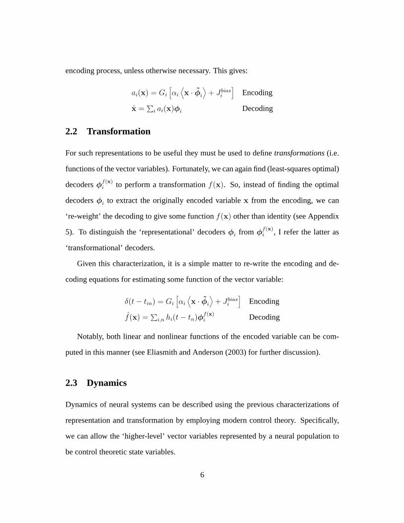
encoding process, unless otherwise necessary. This gives:

ai(x) = Gi

[αi

⟨x · φi

⟩+ J bias

i

]Encoding

x =∑

i ai(x)φi Decoding

2.2 Transformation

For such representations to be useful they must be used to definetransformations(i.e.

functions of the vector variables). Fortunately, we can again find (least-squares optimal)

decodersφf(x)i to perform a transformationf(x). So, instead of finding the optimal

decodersφi to extract the originally encoded variablex from the encoding, we can

‘re-weight’ the decoding to give some functionf(x) other than identity (see Appendix

5). To distinguish the ‘representational’ decodersφi from φf(x)i , I refer the latter as

‘transformational’ decoders.

Given this characterization, it is a simple matter to re-write the encoding and de-

coding equations for estimating some function of the vector variable:

δ(t − tin) = Gi

[αi

⟨x · φi

⟩+ J bias

i

]Encoding

f(x) =∑

i,n hi(t − tn)φf(x)i Decoding

Notably, both linear and nonlinear functions of the encoded variable can be com-

puted in this manner (see Eliasmith and Anderson (2003) for further discussion).

2.3 Dynamics

Dynamics of neural systems can be described using the previous characterizations of

representation and transformation by employing modern control theory. Specifically,

we can allow the ‘higher-level’ vector variables represented by a neural population to

be control theoretic state variables.

6

Let us first consider linear, time-invariant (LTI) systems. Recall that the state equa-

tion in modern control theory describing LTI dynamics is

x(t) = Ax(t) + Bu(t). (5)

The input matrixB and the dynamics matrixA completely describe the dynamics of

the LTI system, given the state variablesx(t) and the inputu(t). Taking the Laplace

transform of (5) gives:

x(s) = h(s) [Ax(s) + Bu(s)] ,

whereh(s) = 1s. Any LTI control system can be written in this form.

In the case of the neural system, the transfer functionh(s) is not 1s, but is determined

by the intrinsic properties of the component cells. Because it is reasonable to assume

that the dynamics of the synaptic PSC dominate the dynamics of the cellular response

as a whole (Eliasmith and Anderson 2003), it is reasonable to characterize the dynamics

of neural populations based on their synaptic dynamics, i.e. usinghi(t) from (4).

A simple model of a PSC is given by

h′(t) =1

τe−t/τ , (6)

whereτ is the synaptic time constant. The Laplace transform of this filter is:

h′(s) =1

1 + sτ.

Given the change in filters fromh(s) to h′(s), we now need to determine how to

changeA andB in order to preserve the dynamics defined in the original system (i.e.

7

the one usingh(s)). In other words, letting the neural dynamics be defined byA′ and

B′, we need to determine the relation between matricesA andA′ and matricesB and

B′ given the differences betweenh(s) andh′(s). To do so, we can solve forx(s) in

both cases and equate the resulting expressions forx(s). Doing so gives

A′ = τA + I (7)

B′ = τB. (8)

This procedure assumes nothing aboutA or B, so we can construct a neurobiolog-

ically realistic implementations of any dynamical system defined using the techniques

of modern control theory applied to LTI systems (constrained by the neurons’ intrinsic

dynamics). Note also that this derivation is independent of the spiking nonlinearity,

since that process is both very rapid, and dedicated to encoding the resultant somatic

voltage (not filtering it in any significant way). Importantly, the same approach can be

used to characterize the broader class of time-varying and nonlinear control systems,

which I provide examples of below.

2.4 Synthesis

Combining the preceding characterizations of representation, transformation, and dy-

namics results in the generic neural subsystem shown in figure 1. With this formula-

tion, the synaptic weights needed to implement some specified control system can be

directly computed. Note that the formulation also provides for simulating the same

model at various levels of description (e.g., at the level of neural populations or indi-

vidual neurons, using either rate neurons or spiking neurons, and so on). This is useful

for fine-tuning a model before introducing the extra computational overhead involved

8

Mab

Mab'

1 fjFb

fjFb'

fia Gi[.]

... ... ... ...

Jia(t)

synaptic weights

soma

higher-level�description

neural description

1

~

PSCs

dendrites

Fab[xb(t)]

Fab'[xb'(t)]1+stij

Sda(t-tin)n

Sdb(t-tjn)n

Sdb'(t-tjn)nab'

1+stijab

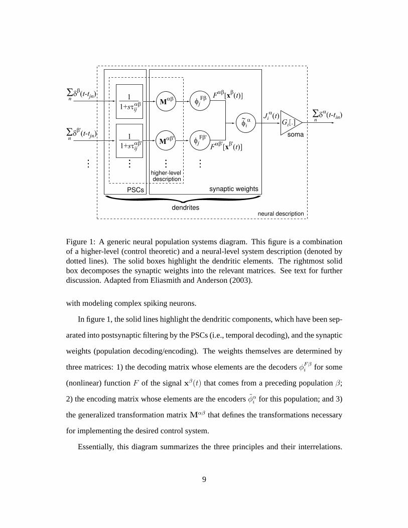
Figure 1: A generic neural population systems diagram. This figure is a combinationof a higher-level (control theoretic) and a neural-level system description (denoted bydotted lines). The solid boxes highlight the dendritic elements. The rightmost solidbox decomposes the synaptic weights into the relevant matrices. See text for furtherdiscussion. Adapted from Eliasmith and Anderson (2003).

with modeling complex spiking neurons.

In figure 1, the solid lines highlight the dendritic components, which have been sep-

arated into postsynaptic filtering by the PSCs (i.e., temporal decoding), and the synaptic

weights (population decoding/encoding). The weights themselves are determined by

three matrices: 1) the decoding matrix whose elements are the decodersφFβi for some

(nonlinear) functionF of the signalxβ(t) that comes from a preceding populationβ;

2) the encoding matrix whose elements are the encodersφαi for this population; and 3)

the generalized transformation matrixMαβ that defines the transformations necessary

for implementing the desired control system.

Essentially, this diagram summarizes the three principles and their interrelations.

9

The generality of the diagram hints at the generality of the underlying framework. In

the remainder of the paper, however, I focus only on its application to the construction

and control of attractor networks.

3 Building attractor networks

The most obvious feature of attractor networks is their tendency towards dynamic sta-

bility. That is, given a momentary input, they will ‘settle’ on a position, or a recurring

sequence of positions, in state space. This kind of stability can be usefully exploited by

biological systems in a number of ways. For instance, it can help a system react to envi-

ronmental changes on multiple time scales. That is, stability permits systems to act on

longer time scales than they might otherwise be able to, which is essential for numerous

behaviors including prediction, navigation, and social interaction. In addition, stability

can be used as an indicator of task completion, such as in the case of stimulus cate-

gorization (Hopfield 1982). As well, stability can make the system more robust; i.e.,

more resistant to undesirable perturbations. Because these networks are constructed so

as to have only a certain set of stable states, random perturbations to nearby states can

quickly dissipate to a stable state. As a result, attractor networks have been shown to be

effective for noise reduction (Pouget et al. 1998). Similarly, attractors over a series of

states (e.g. cyclic attractors) can be used to robustly support repetitive behaviors such

as walking, swimming, flying, or chewing.

Given these kinds of useful computational properties, and their natural analogs in

biological behavior, it is unsurprising that attractor networks have become a staple of

computational neuroscience. More than this, as the complexity of computational mod-

els continues to increase, attractor networks are likely to form important sub-networks

10

in larger models. This is because the ability of attractor networks to, for example, cat-

egorize, filter noise, and integrate signals, makes them good candidates for being some

of the basic building blocks of complex signal processing systems. As a result, the

networks described here should prove useful for a wide class of more complex models.

To maintain consistency, all of the results of subsequent models were generated

using networks of leaky integrate-and-fire neurons with absolute refractory periods of

1ms, membrane time constants of10ms, and synaptic time constants of5ms.1 Intercepts

and maximum firing rates were chosen from even distributions. The intercept intervals

are normalized over[−1, 1] unless otherwise specified. For a detailed discussion of the

effects of changing these parameters, see Eliasmith and Anderson (2003).

For each example presented below, the presentation focuses specifically on thecon-

structionof the relevant model. As a result, there is minimal discussion of the jus-

tification for mapping particular kinds of attractors onto various neural systems and

behaviors, although references are provided.

3.1 Line attractor

The line attractor, or ‘neural integrator’, has recently been implicated in decision mak-

ing (Shadlen and Newsome 2001), but most extensively explored in the context of ocu-

lomotor control (Fukushima et al. 1992; Seung 1996; Askay et al. 2001). It is in-

teresting to note that the terms ‘line attractor’ and ‘neural integrator’ actually describe

different aspects of the network. In particular, the network is called an ‘integrator’ be-

cause the low-dimensional variable (e.g., horizontal eye position)x(t) describing the

network’s output reflects the integration of the input signal (e.g., eye movement veloc-

1Note that this choice of a very short synaptic time constant makes it more difficult to achieve stabilityin recurrent networks. Many models assume synaptic time constants on the order of 100ms or longer.

11

u(t)

x(t)

A

B

bk(t) aj(t)

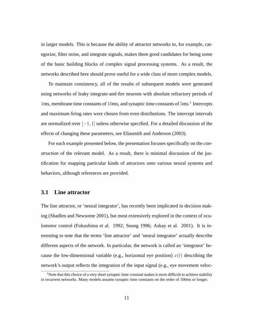
Figure 2: Line attractor network architecture. The underline denotes variables that arepart of the neuron-level description. The remaining variables are part of the higher-leveldescription.

ity) u(t) to the system. In contrast, the network is called a ‘line attractor’ because in

the high-dimensional activity space of the network (where the dimension is equal to the

number of neurons in the network), the organization of the system collapses network

activity to lie on a one-dimensional subspace (i.e. a line). As a result, only input that

moves the network along this line changes the network’s output.

In a sense, then, these two terms reflect a difference between what can be called

‘higher-level’ and ‘neuron-level’ descriptions of the system (see figure 2). As modelers

of this system, we need a method that allows us to integrate these two descriptions.

Adopting the principles outlined earlier does precisely this. Notably, the resulting

derivation is extremely simple, and is similar to that already presented in Eliasmith

and Anderson (2003). However, all of the steps need to generate the far more complex

circuits discussed later are described here, so it is a useful introduction (and refered to

for some of the subsequent derivations).

We can begin by describing the higher-level behavior as integration, which has the

state equation

12

x = Ax(t) + Bu(t) (9)

x(s) =1

s[Ax(s) + Bu(s)] , (10)

whereA = 0 andB = 1. Given principle 3, we can determine theA′ andB′, which are

needed to implement this behavior in a system with neural dynamics defined byh′(t)

(see (6)). The result is

B′ = τ

A′ = 1,

whereτ is the time constant of the PSC of neurons in the population representingx(t).

To use this description in a neural model, we must define the representation of the

state variable of the system, i.e.,x(t). Given principle 1, let us define this representation

using the following encoding and decoding:

aj(t) = Gj

[αj

⟨x(t)φj

⟩+ J bias

j

](11)

and

x(t) =∑j

aj(t)φxj . (12)

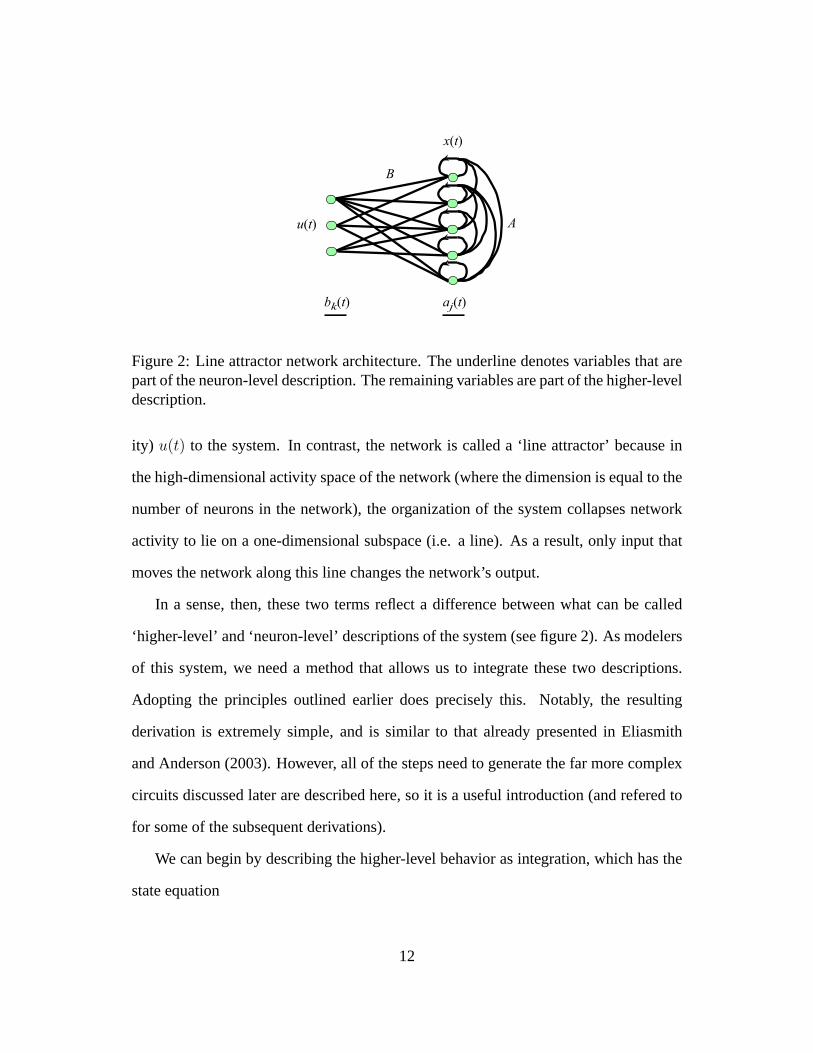
Note that the encoding weightφj plays the same role as the encoding vector in (2), but

is simply±1 (for ‘on’ and ‘off’ neurons) in the scalar case. Figure 3 shows a population

of neurons with this kind of encoding. Let us also assume an analogous representation

for u(t).

13

-1 -0.8 -0.6 -0.4 -0.2 0 0.2 0.4 0.6 0.8 10

50

100

150

200

250

x

Fir

ing

Rat

e (H

z)

Figure 3: Sample tuning curves for a population of neurons used to implement theline attractor. These are the equivalent steady state tuning curves of the spiking neu-rons used in this example. They are found by solving the differential equations forthe LIF neuron assuming a constant input current, and are described by:aj(x) =

1

τrefj −τRC

j ln

(1− Jthreshold

αjx+Jbias

) .

14

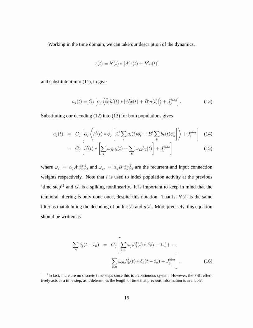
Working in the time domain, we can take our description of the dynamics,

x(t) = h′(t) ∗ [A′x(t) + B′u(t)]

and substitute it into (11), to give

aj(t) = Gj

[αj

⟨φjh

′(t) ∗ [A′x(t) + B′u(t)]⟩

+ J biasj

]. (13)

Substituting our decoding (12) into (13) for both populations gives

aj(t) = Gj

[αj

⟨h′(t) ∗ φj

[A′∑

i

ai(t)φxi + B′∑

k

bk(t)φuk

]⟩+ J bias

j

](14)

= Gj

[h′(t) ∗

[∑i

ωjiai(t) +∑k

ωjkbk(t)

]+ J bias

j

](15)

whereωji = αjA′φx

i φj andωjk = αjB′φu

kφj are the recurrent and input connection

weights respectively. Note thati is used to index population activity at the previous

‘time step’2 andGi is a spiking nonlinearity. It is important to keep in mind that the

temporal filtering is only done once, despite this notation. That is,h′(t) is the same

filter as that defining the decoding of bothx(t) andu(t). More precisely, this equation

should be written as

∑n

δj(t − tn) = Gj

∑i,n

ωjih′i(t) ∗ δi(t − tn)+ ...

∑k,n

ωjkh′k(t) ∗ δk(t − tn) + J bias

j

. (16)

2In fact, there are no discrete time steps since this is a continuous system. However, the PSC effec-tively acts as a time step, as it determines the length of time that previous information is available.

15

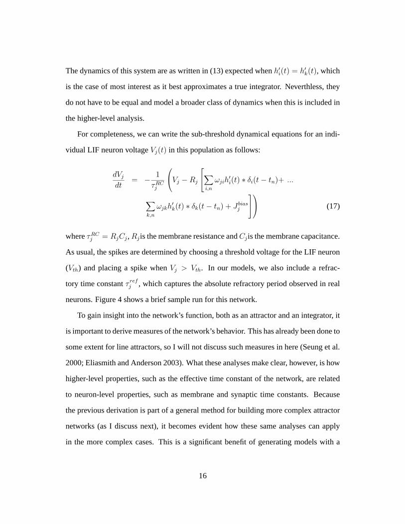
The dynamics of this system are as written in (13) expected whenh′i(t) = h′

k(t), which

is the case of most interest as it best approximates a true integrator. Neverthless, they

do not have to be equal and model a broader class of dynamics when this is included in

the higher-level analysis.

For completeness, we can write the sub-threshold dynamical equations for an indi-

vidual LIF neuron voltageVj(t) in this population as follows:

dVj

dt= − 1

τRCj

Vj − Rj

∑i,n

ωjih′i(t) ∗ δi(t − tn)+ ...

∑k,n

ωjkh′k(t) ∗ δk(t − tn) + J bias

j

(17)

whereτRCj = RjCj, Rj is the membrane resistance andCj is the membrane capacitance.

As usual, the spikes are determined by choosing a threshold voltage for the LIF neuron

(Vth) and placing a spike whenVj > Vth. In our models, we also include a refrac-

tory time constantτ refj , which captures the absolute refractory period observed in real

neurons. Figure 4 shows a brief sample run for this network.

To gain insight into the network’s function, both as an attractor and an integrator, it

is important to derive measures of the network’s behavior. This has already been done to

some extent for line attractors, so I will not discuss such measures in here (Seung et al.

2000; Eliasmith and Anderson 2003). What these analyses make clear, however, is how

higher-level properties, such as the effective time constant of the network, are related

to neuron-level properties, such as membrane and synaptic time constants. Because

the previous derivation is part of a general method for building more complex attractor

networks (as I discuss next), it becomes evident how these same analyses can apply

in the more complex cases. This is a significant benefit of generating models with a

16

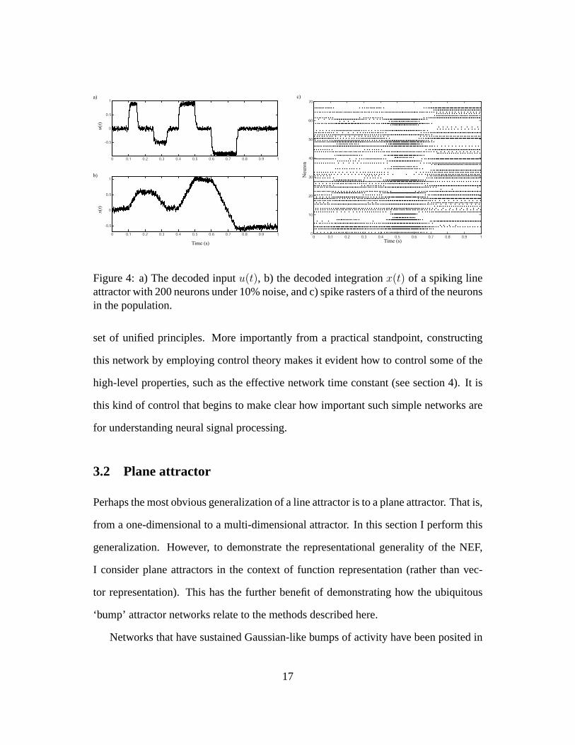
0 0.1 0.2 0.3 0.4 0.5 0.6 0.7 0.8 0.9 1

-0.5

0

0.5

1

0 0.1 0.2 0.3 0.4 0.5 0.6 0.7 0.8 0.9 1

-0.5

0

0.5

1

u(t

)x(t

)a)

b)

Time (s)

0 0.1 0.2 0.3 0.4 0.5 0.6 0.7 0.8 0.9 10

10

20

30

40

50

60

70

Neu

ron

Time (s)

c)

Figure 4: a) The decoded inputu(t), b) the decoded integrationx(t) of a spiking lineattractor with 200 neurons under 10% noise, and c) spike rasters of a third of the neuronsin the population.

set of unified principles. More importantly from a practical standpoint, constructing

this network by employing control theory makes it evident how to control some of the

high-level properties, such as the effective network time constant (see section 4). It is

this kind of control that begins to make clear how important such simple networks are

for understanding neural signal processing.

3.2 Plane attractor

Perhaps the most obvious generalization of a line attractor is to a plane attractor. That is,

from a one-dimensional to a multi-dimensional attractor. In this section I perform this

generalization. However, to demonstrate the representational generality of the NEF,

I consider plane attractors in the context of function representation (rather than vec-

tor representation). This has the further benefit of demonstrating how the ubiquitous

‘bump’ attractor networks relate to the methods described here.

Networks that have sustained Gaussian-like bumps of activity have been posited in

17

various neural systems including frontal working memory areas (Laing and Chow 2001;

Brody et al. 2003), the head direction system (Zhang 1996; Redish 1999), visual feature

selection areas (Hansel and Sompolinsky 1998), and arm control systems (Snyder et al.

1997). The prevalence of this kind of attractor suggests that it is important to account

for such networks in a general framework. However, it is not immediately obvious how

the stable representation of functions relates to either vector or scalar representation as

I have so far described it.

Theoretically, continuous function representation demands an infinite number of

degrees of freedom. Neural systems, of course, are finite. As a result, it is natural to

assume that understanding function representation in neural systems can be done using

a finite basis for the function space accessible by that system. Given a finite basis,

the finite set of coefficients of such a basis determine the function being represented

by the system at any time. As a result, function representation can be treated as the

representation of avectorof coefficients over some basis. That is,

x(ν;A) =M∑

m=1

xmΦm(ν) (18)

whereνis the dimension the function is defined over (e.g., spatial position),xis the

vector ofM coefficientsxm, andΦm are the set ofM orthonormal basis functions

needed to define the function space. Notably, this basis does not need to be accessible

in any way by the neural system itself, it is merely a way for us to conveniently write

the function space that is represented by the system.

The neural representation depends on an overcomplete representation of this same

space, where the overcomplete basis is defined by the tuning curves of the relevant

neurons. More specifically, we can define the encoding of a function space analogously

18

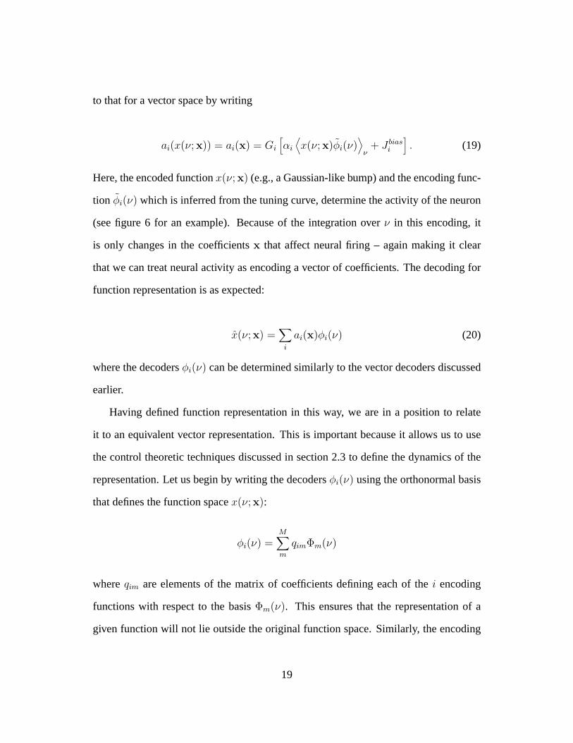
to that for a vector space by writing

ai(x(ν;x)) = ai(x) = Gi

[αi

⟨x(ν;x)φi(ν)

⟩ν

+ J biasi

]. (19)

Here, the encoded functionx(ν;x) (e.g., a Gaussian-like bump) and the encoding func-

tion φi(ν) which is inferred from the tuning curve, determine the activity of the neuron

(see figure 6 for an example). Because of the integration overν in this encoding, it

is only changes in the coefficientsx that affect neural firing – again making it clear

that we can treat neural activity as encoding a vector of coefficients. The decoding for

function representation is as expected:

x(ν;x) =∑

i

ai(x)φi(ν) (20)

where the decodersφi(ν) can be determined similarly to the vector decoders discussed

earlier.

Having defined function representation in this way, we are in a position to relate

it to an equivalent vector representation. This is important because it allows us to use

the control theoretic techniques discussed in section 2.3 to define the dynamics of the

representation. Let us begin by writing the decodersφi(ν) using the orthonormal basis

that defines the function spacex(ν;x):

φi(ν) =M∑m

qimΦm(ν)

whereqim are elements of the matrix of coefficients defining each of thei encoding

functions with respect to the basisΦm(ν). This ensures that the representation of a

given function will not lie outside the original function space. Similarly, the encoding

19

functionsφi(ν) should only encode functionsx(ν;x) in such a way that they can be

decoded by these decoders, so we may assume

φi(ν) =M∑m

qimΦm(ν). (21)

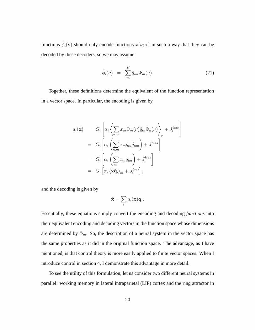
Together, these definitions determine the equivalent of the function representation

in a vector space. In particular, the encoding is given by

ai(x) = Gi

αi

⟨∑n,m

xmΦm(ν)qinΦn(ν)

⟩ν

+ J biasi

= Gi

[αi

(∑n,m

xmqinδnm

)+ J bias

i

]

= Gi

[αi

(∑m

xmqim

)+ J bias

i

]= Gi

[αi 〈xqi〉m + J bias

i

],

and the decoding is given by

x =∑

i

ai(x)qi.

Essentially, these equations simply convert the encoding and decodingfunctionsinto

their equivalent encoding and decoding vectors in the function space whose dimensions

are determined byΦm. So, the description of a neural system in the vector space has

the same properties as it did in the original function space. The advantage, as I have

mentioned, is that control theory is more easily applied to finite vector spaces. When I

introduce control in section 4, I demonstrate this advantage in more detail.

To see the utility of this formulation, let us consider two different neural systems in

parallel: working memory in lateral intraparietal (LIP) cortex and the ring attractor in

20

-1 -0.8 -0.6 -0.4 -0.2 0 0.2 0.4 0.6 0.8 1

-0.1

-0.05

0

0.05

0.1

ν

Φ(ν)

Φ1

Φ2

Φ3

Φ4

Φ5

-3 -2 -1 0 1 2 3-0.1

-0.08

-0.06

-0.04

-0.02

0

0.02

0.04

0.06

0.08

0.1

ν

Φ1

Φ2

Φ3

Φ4

Φ5

a) b)Φ(ν)

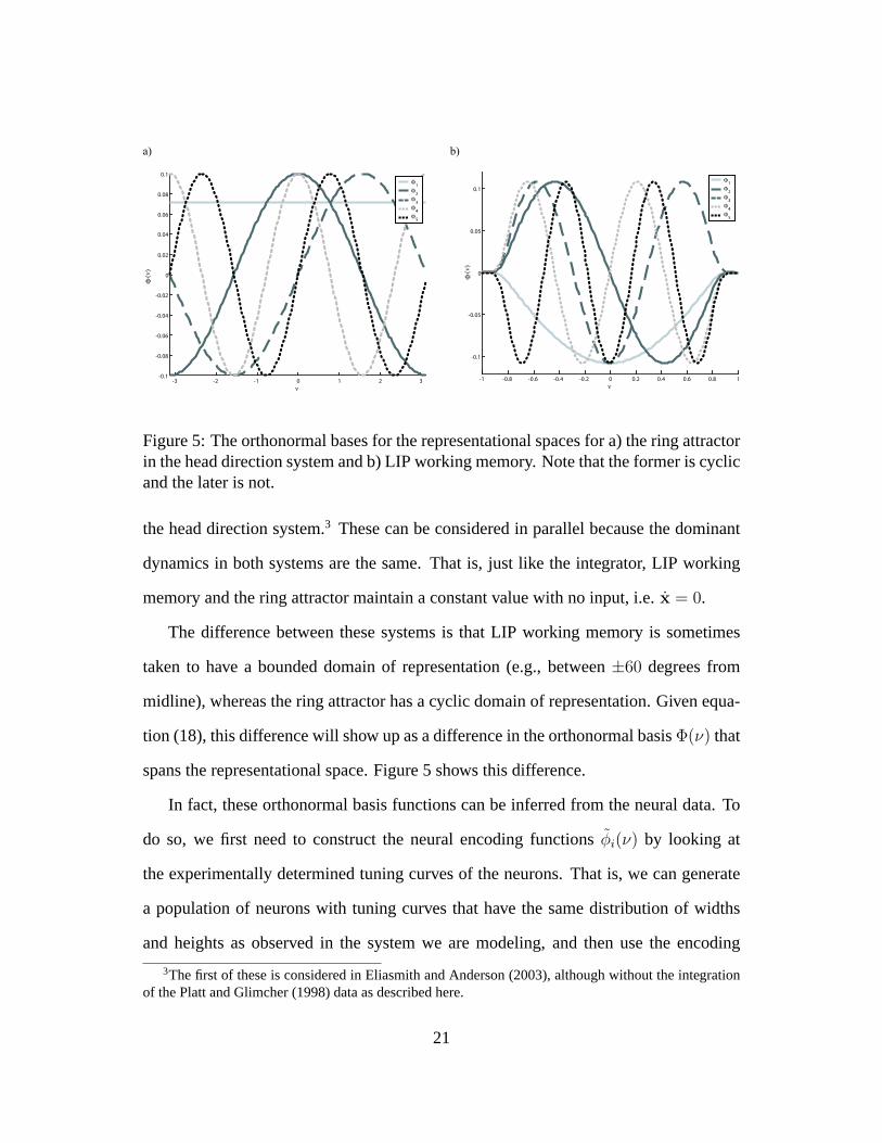
Figure 5: The orthonormal bases for the representational spaces for a) the ring attractorin the head direction system and b) LIP working memory. Note that the former is cyclicand the later is not.

the head direction system.3 These can be considered in parallel because the dominant

dynamics in both systems are the same. That is, just like the integrator, LIP working

memory and the ring attractor maintain a constant value with no input, i.e.x = 0.

The difference between these systems is that LIP working memory is sometimes

taken to have a bounded domain of representation (e.g., between±60 degrees from

midline), whereas the ring attractor has a cyclic domain of representation. Given equa-

tion (18), this difference will show up as a difference in the orthonormal basisΦ(ν) that

spans the representational space. Figure 5 shows this difference.

In fact, these orthonormal basis functions can be inferred from the neural data. To

do so, we first need to construct the neural encoding functionsφi(ν) by looking at

the experimentally determined tuning curves of the neurons. That is, we can generate

a population of neurons with tuning curves that have the same distribution of widths

and heights as observed in the system we are modeling, and then use the encoding

3The first of these is considered in Eliasmith and Anderson (2003), although without the integrationof the Platt and Glimcher (1998) data as described here.

21

60 40 20 0 20 40 600

20

40

60

80

100

120

140

160

180

ν (degrees)

Fir

ing R

ate

(Hz)

0

0.05

0.1

0.15

0.2

0.25

60 40 20 0 20 40 60ν (degrees)

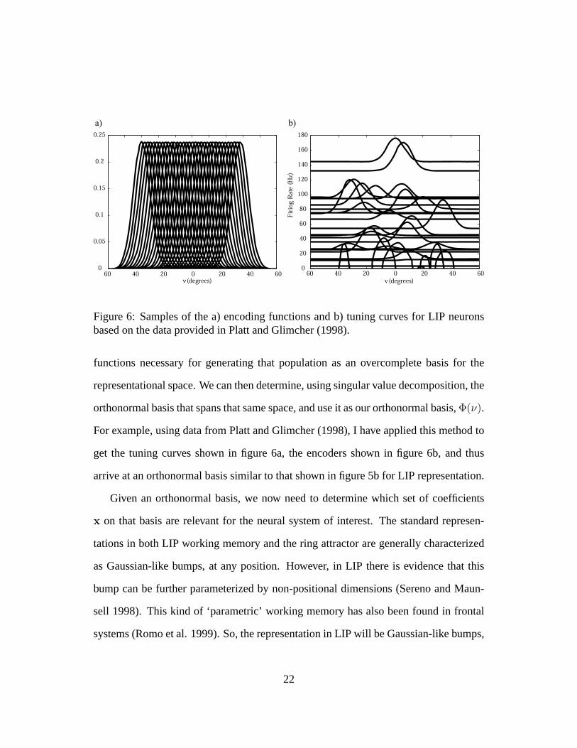
a) b)

Figure 6: Samples of the a) encoding functions and b) tuning curves for LIP neuronsbased on the data provided in Platt and Glimcher (1998).

functions necessary for generating that population as an overcomplete basis for the

representational space. We can then determine, using singular value decomposition, the

orthonormal basis that spans that same space, and use it as our orthonormal basis,Φ(ν).

For example, using data from Platt and Glimcher (1998), I have applied this method to

get the tuning curves shown in figure 6a, the encoders shown in figure 6b, and thus

arrive at an orthonormal basis similar to that shown in figure 5b for LIP representation.

Given an orthonormal basis, we now need to determine which set of coefficients

x on that basis are relevant for the neural system of interest. The standard represen-

tations in both LIP working memory and the ring attractor are generally characterized

as Gaussian-like bumps, at any position. However, in LIP there is evidence that this

bump can be further parameterized by non-positional dimensions (Sereno and Maun-

sell 1998). This kind of ‘parametric’ working memory has also been found in frontal

systems (Romo et al. 1999). So, the representation in LIP will be Gaussian-like bumps,

22

but of varying heights.

Ideally, we need to specify some probability densityρ(x) on the coefficients that

appropriately picks out just the Gaussian-like functions centered at every value ofν

(and those of various heights for the LIP model). This essentially specifies the range of

functions that are permissible in our function space. It is clearly undesirable to have all

functions that can be represented by the orthonormal basis as candidate representations.

Givenρ(x) we can use the methods described in appendix 5 to find the decoders. In

particular, the average overx in equation (31) is replaced by an average overρ(x). In

practice, it can be difficult to compactly defineρ(x), so it is often convenient to use a

Monte Carlo method for approximating this distribution when performing the average,

which I have done for these examples.

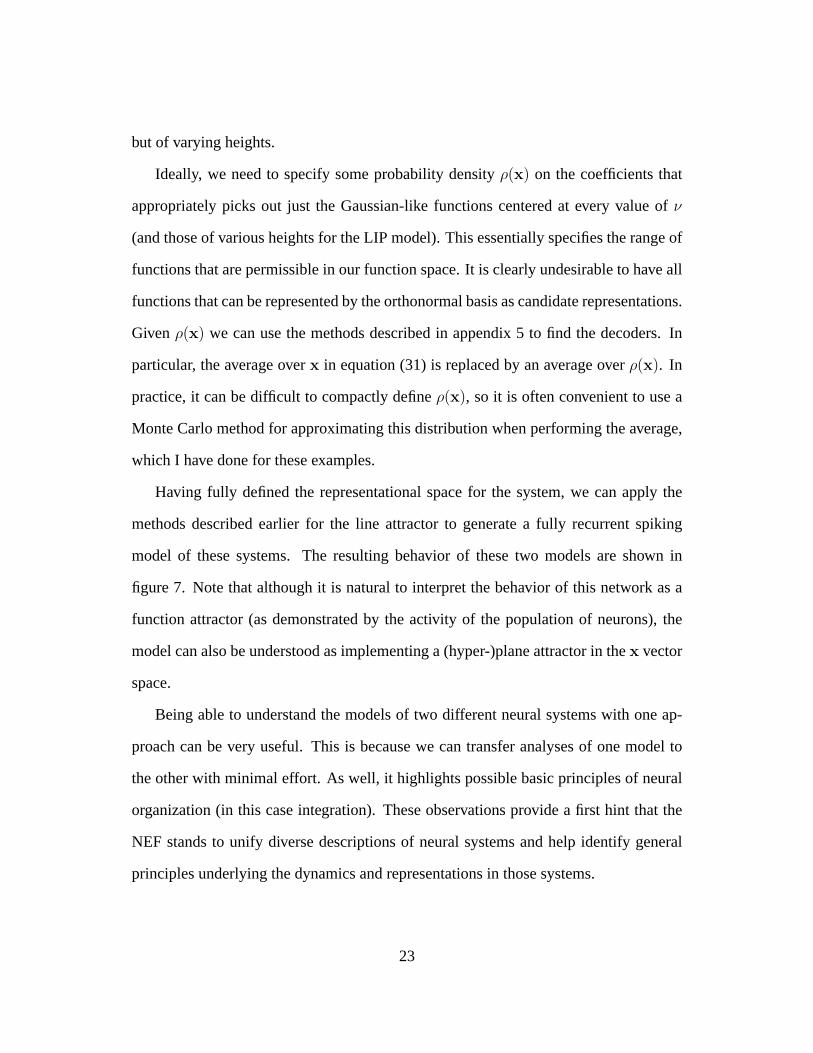
Having fully defined the representational space for the system, we can apply the

methods described earlier for the line attractor to generate a fully recurrent spiking

model of these systems. The resulting behavior of these two models are shown in

figure 7. Note that although it is natural to interpret the behavior of this network as a

function attractor (as demonstrated by the activity of the population of neurons), the

model can also be understood as implementing a (hyper-)plane attractor in thex vector

space.

Being able to understand the models of two different neural systems with one ap-

proach can be very useful. This is because we can transfer analyses of one model to

the other with minimal effort. As well, it highlights possible basic principles of neural

organization (in this case integration). These observations provide a first hint that the

NEF stands to unify diverse descriptions of neural systems and help identify general

principles underlying the dynamics and representations in those systems.

23

π

ν-π-101

0

0.5

1

Tim

e (s)

ν

a) b)

0

10005001

0

0.5

1

Tim

e (s)

Neuron

10005001

Neuron

Figure 7: Simulation results for a) LIP working memory encoding two different bumpheights at two locations and b) a head-direction ring attractor. The top graph showsthe decoded function representation, and the bottom graph shows the activity of theneurons in the population (the activity plots are calculated from spiking data using a20ms time window with background activity removed, and are smoothed by a 50 pointmoving average). Both models use 1000 spiking LIF neurons with 10% noise added.

24

3.3 Cyclic attractor

The kinds of attractors I have presented to this point are, in a sense, static because once

the system has settled to a stable point, it will remain there unless perturbed. However,

there is another broad class of attractors that have dynamic, periodic stability. In such

cases, settling into the attractor results in a cyclic progression through a closed set of

points. The simplest example of this kind of attractor is the ideal oscillator.

Because cyclic attractors are used to describe oscillators, and many neural systems

seem to include oscillatory behavior, it is natural to use cyclic attractors to describe os-

cillatory behavior in neural systems. Such behavior may include any repetitive motion

such as walking, swimming, flying, chewing, and so on. The natural mapping between

oscillators and repetitive behavior is at the heart of most work on central pattern gener-

ators (CPGs; Selverston 1980; Kopell and Ermentrout 1988). However, this work typi-

cally characterizes oscillators as interactions between only a few neighboring neurons.

In contrast, the NEF can help us in understanding cyclic attractors at the network level.

Comparing the results of a NEF characterization with that of the standard approach to

CPGs shows that there are advantages to the higher-level characterization. To effect

this comparison, let us extend a previously described model of lamprey swimming (for

more detail of the mechanical model, see Eliasmith and Anderson 2000; Eliasmith and

Anderson 2003).4 Later, I extend this model by introducing control.

When the lamprey swims, the resulting motion resembles a standing wave of one

period over the lamprey’s length. The tensionsT in the muscles needed to give rise to

4Unlike the previous model, this one includes noisy spiking neurons. Parameters for these neuronsand their distribution are based on data in Manira et al. (1994). This effectivley demonstrates that thebursting observed in lamprey spinal cord is observed in the model as well.

25

this motion can be described by:

T (z, t) = κ(sin(ωt − kz) − sin(ωt)), (22)

whereκ = γηωAk

, k = 2πL

, A = 1 is the wave amplitude,η = 1 is the normalized

viscosity coefficient,γ = 1 is the ratio of intersegmental and vertebrae length,L = 1

is the length of the lamprey, andω is the swimming frequency.

As for the LIP model, we can define an orthogonal representation of the dynamic

pattern of tensions in terms of the coefficientsxn(t) and the harmonic functionsΦn(z):

T (z, t;x) = κ

(x0 +

N∑n=1

x2n−1(t) sin(2πnz) + x2n(t) cos(2πnz)

).

The appropriatex coefficients are found by setting the MSE betweenT (z, t;x) and

T (z, t) to be zero. Doing so, we find thatx0(t) = − sin(ωt), x1(t) = − cos(ωt),

x2(t) = sin(ωt), and forn > 2, xn(t) = 0. This defines the representation in a higher-

level function space, whose dynamics we can implement by describing the dynamics

of the coefficients,x.

In this case, it is evident that the coefficientsx0andx1implement a standard oscil-

lator. The coefficientx2 is an additional counter-phase sine wave. This additional term

simply tilts the 2-dimensional cyclic attractor in phase space, so we essentially have

just a standard oscillator. We can write the control equations as usual

x = Ax

26

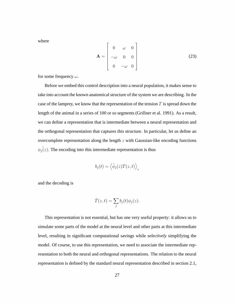
where

A =

0 ω 0

−ω 0 0

0 −ω 0

(23)

for some frequencyω.

Before we embed this control description into a neural population, it makes sense to

take into account the known anatomical structure of the system we are describing. In the

case of the lamprey, we know that the representation of the tensionT is spread down the

length of the animal in a series of 100 or so segments (Grillner et al. 1991). As a result,

we can define a representation that is intermediate between a neural representation and

the orthogonal representation that captures this structure. In particular, let us define an

overcomplete representation along the lengthz with Gaussian-like encoding functions

˜φj(z). The encoding into this intermediate representation is thus

bj(t) =⟨φj(z)T (z, t)

⟩z

and the decoding is

T (z, t) =∑j

bj(t)φj(z).

This representation is not essential, but has one very useful property: it allows us to

simulate some parts of the model at the neural level and other parts at this intermediate

level, resulting in significant computational savings whileselectivelysimplifying the

model. Of course, to use this representation, we need to associate the intermediate rep-

resentation to both the neural and orthogonal representations. The relation to the neural

representation is defined by the standard neural representation described in section 2.1,

27

with the encoding given by

δ(t − tin) = Gi

[αi

⟨bjφi

⟩+ J bias

i

]

and the decoding by

bj =∑i,n

hij(t − tn)φi.

Essentially, these equations describe how the intermediate population activitybj is re-

lated to the actual neurons, indexed byi, in the various populations along the length of

the lamprey.5

To relate the intermediate and orthogonal spaces, we can use the projection oper-

ator Θ =[φΦ]. That is, we can project the high-level control description into the

intermediate-level space as follows:

x = Ax

ΘΘ−1b = ΘAΘ−1b

b = Abb

whereAb = ΘAΘ−1.

Having provided these descriptions, we can now selectively convert segments of

the intermediate representation into spiking neurons to see how single cells perform in

the context of the whole, dynamic spinal cord. Figure 8a shows single cells that burst

during swimming, and figure 8b shows the average spike rate of an entire population of

5Because the lamprey spinal cord is effectively continuous, assignment of neurons to particular pop-ulations is somewhat arbitrary, although constrained by the part of the lamprey over which they encodemuscle tension. So, the resulting model is similarly continuous as well.

28

a) b)

0 0.5 1 1.5 2 2.5 30

0.5

1

1.5

2

2.5

3

3.5

Time (s)

Fir

ing

Rate

(H

z)

Left sideRight Side

0 0.5 1 1.5 2 2.50

5

10

15

20

Spikes for Single Left/Right Neurons

Time (s)

Neu

ron

Left sideRight Side

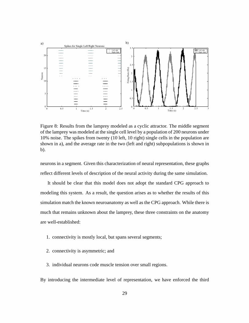
Figure 8: Results from the lamprey modeled as a cyclic attractor. The middle segmentof the lamprey was modeled at the single cell level by a population of 200 neurons under10% noise. The spikes from twenty (10 left, 10 right) single cells in the population areshown in a), and the average rate in the two (left and right) subpopulations is shown inb).

neurons in a segment. Given this characterization of neural representation, these graphs

reflect different levels of description of the neural activity during the same simulation.

It should be clear that this model does not adopt the standard CPG approach to

modeling this system. As a result, the question arises as to whether the results of this

simulation match the known neuroanatomy as well as the CPG approach. While there is

much that remains unknown about the lamprey, these three constraints on the anatomy

are well-established:

1. connectivity is mostly local, but spans several segments;

2. connectivity is asymmetric; and

3. individual neurons code muscle tension over small regions.

By introducing the intermediate level of representation, we have enforced the third

29

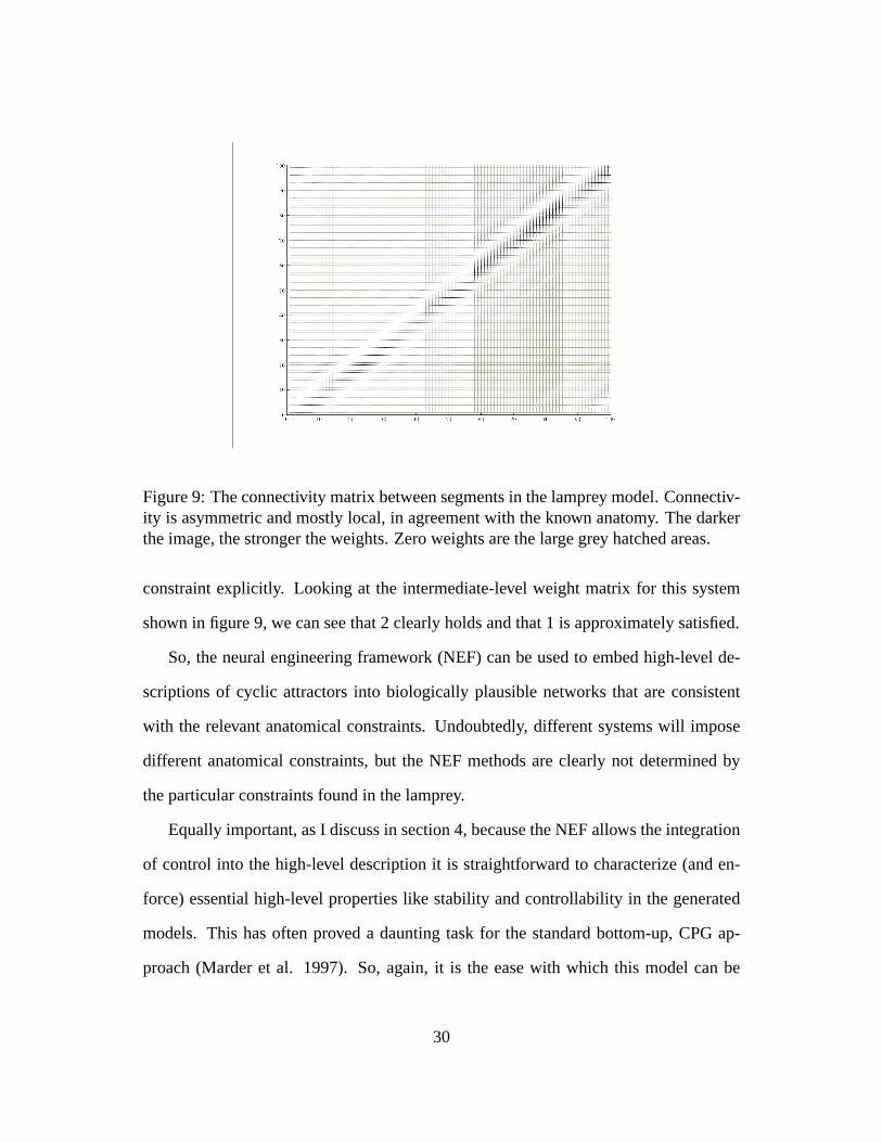
Figure 9: The connectivity matrix between segments in the lamprey model. Connectiv-ity is asymmetric and mostly local, in agreement with the known anatomy. The darkerthe image, the stronger the weights. Zero weights are the large grey hatched areas.

constraint explicitly. Looking at the intermediate-level weight matrix for this system

shown in figure 9, we can see that 2 clearly holds and that 1 is approximately satisfied.

So, the neural engineering framework (NEF) can be used to embed high-level de-

scriptions of cyclic attractors into biologically plausible networks that are consistent

with the relevant anatomical constraints. Undoubtedly, different systems will impose

different anatomical constraints, but the NEF methods are clearly not determined by

the particular constraints found in the lamprey.

Equally important, as I discuss in section 4, because the NEF allows the integration

of control into the high-level description it is straightforward to characterize (and en-

force) essential high-level properties like stability and controllability in the generated

models. This has often proved a daunting task for the standard bottom-up, CPG ap-

proach (Marder et al. 1997). So, again, it is the ease with which this model can be

30

extended to account for important, but complex behaviors that demonstrates the utility

of the NEF.

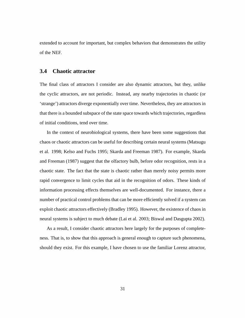
3.4 Chaotic attractor

The final class of attractors I consider are also dynamic attractors, but they, unlike

the cyclic attractors, are not periodic. Instead, any nearby trajectories in chaotic (or

‘strange’) attractors diverge exponentially over time. Nevertheless, they are attractors in

that there is a bounded subspace of the state space towards which trajectories, regardless

of initial conditions, tend over time.

In the context of neurobiological systems, there have been some suggestions that

chaos or chaotic attractors can be useful for describing certain neural systems (Matsugu

et al. 1998; Kelso and Fuchs 1995; Skarda and Freeman 1987). For example, Skarda

and Freeman (1987) suggest that the olfactory bulb, before odor recognition, rests in a

chaotic state. The fact that the state is chaotic rather than merely noisy permits more

rapid convergence to limit cycles that aid in the recognition of odors. These kinds of

information processing effects themselves are well-documented. For instance, there a

number of practical control problems that can be more efficiently solved if a system can

exploit chaotic attractors effectively (Bradley 1995). However, the existence of chaos in

neural systems is subject to much debate (Lai et al. 2003; Biswal and Dasgupta 2002).

As a result, I consider chaotic attractors here largely for the purposes of complete-

ness. That is, to show that this approach is general enough to capture such phenomena,

should they exist. For this example, I have chosen to use the familiar Lorenz attractor,

31

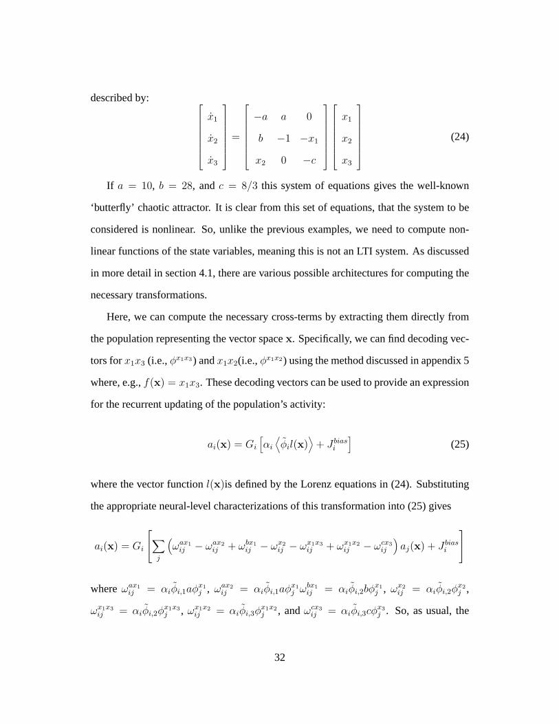
described by: x1

x2

x3

=

−a a 0

b −1 −x1

x2 0 −c

x1

x2

x3

(24)

If a = 10, b = 28, andc = 8/3 this system of equations gives the well-known

‘butterfly’ chaotic attractor. It is clear from this set of equations, that the system to be

considered is nonlinear. So, unlike the previous examples, we need to compute non-

linear functions of the state variables, meaning this is not an LTI system. As discussed

in more detail in section 4.1, there are various possible architectures for computing the

necessary transformations.

Here, we can compute the necessary cross-terms by extracting them directly from

the population representing the vector spacex. Specifically, we can find decoding vec-

tors forx1x3 (i.e.,φx1x3) andx1x2(i.e.,φx1x2) using the method discussed in appendix 5

where, e.g.,f(x) = x1x3. These decoding vectors can be used to provide an expression

for the recurrent updating of the population’s activity:

ai(x) = Gi

[αi

⟨φil(x)

⟩+ J bias

i

](25)

where the vector functionl(x)is defined by the Lorenz equations in (24). Substituting

the appropriate neural-level characterizations of this transformation into (25) gives

ai(x) = Gi

∑j

(ωax1

ij − ωax2ij + ωbx1

ij − ωx2ij − ωx1x3

ij + ωx1x2ij − ωcx3

ij

)aj(x) + J bias

i

whereωax1ij = αiφi,1aφx1

j , ωax2ij = αiφi,1aφx1

j ωbx1ij = αiφi,2bφ

x1j , ωx2

ij = αiφi,2φx2j ,

ωx1x3ij = αiφi,2φ

x1x3j , ωx1x2

ij = αiφi,3φx1x2j , andωcx3

ij = αiφi,3cφx3j . So, as usual, the

32

connection weights are found by combining the encoding and decoding vectors as ap-

propriate. Note that despite implementing a higher-level nonlinear system, there are no

multiplications between neural activities in the neural-level description. This demon-

strates that the neural nonlinearities alone result in the nonlinear behavior of the net-

work. That is, no additional nonlinearities (e.g., dendritic nonlinearities) are needed to

give rise to this behavior.

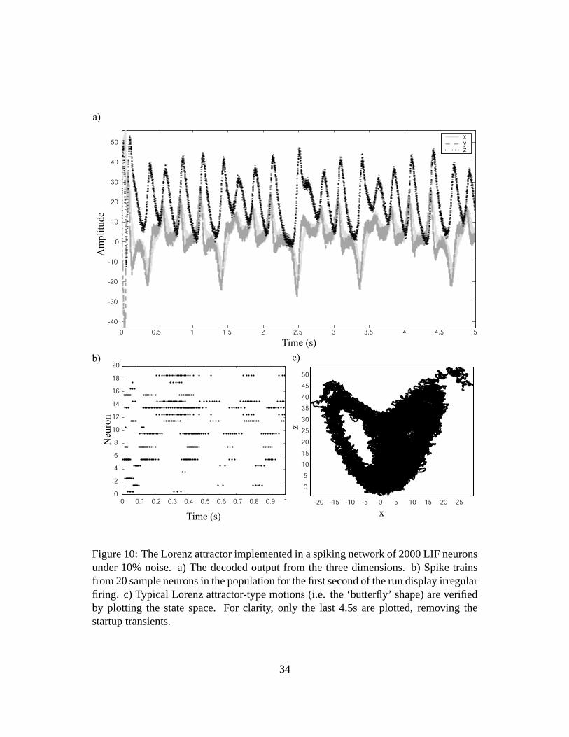
Running this simulation in a spiking network of 2000 LIF neurons under noise gives

the results shown in figure 10. Because this is a simulation of a chaotic network under

noise, it is essential to demonstrate that a chaotic system is in fact being implemented,

and the results are not just noisy spiking from neurons. Applying the noise titration

method (Poon and Barahona 2001) on the decoded spikes verifies the presence of chaos

in the system (P-value <10−15 with a noise limit of 54%, where the noise limit indicates

how much more noise could be added before the nonlinearity was no longer detectable).

Notably, the noise titration method is much better at detecting chaos in time series than

most other methods, even in highly noisy contexts. As a result, we can be confident that

the simulated system is implementing a chaotic attractor as expected. This can also be

qualitatively verified by plotting the state space of the decoded network activity, which

clearly preserves the ‘butterfly’ look of the Lorenz attractor (figure 10c).

4 Controlling attractor networks

To this point I have demonstrated how three main classes of attractor networks can be

embedded into neurobiologically plausible systems, and I have indicated, in each case,

which specific systems might be well-modeled by these various kinds of attractors.

However, in each case, I have not demonstrated how a neural system couldusethis

33

0 0.5 1 1.5 2 2.5 3 3.5 4 4.5 5

-40

-30

-20

-10

0

10

20

30

40

50

Time (s)

xyz

Am

pli

tude

0 0.1 0.2 0.3 0.4 0.5 0.6 0.7 0.8 0.9 10

2

4

6

8

10

12

14

16

18

20

Neu

ron

Time (s)

-20 -15 -10 -5 0 5 10 15 20 25

0

5

10

15

20

25

30

35

40

45

50

z

x

a)

b) c)

Figure 10: The Lorenz attractor implemented in a spiking network of 2000 LIF neuronsunder 10% noise. a) The decoded output from the three dimensions. b) Spike trainsfrom 20 sample neurons in the population for the first second of the run display irregularfiring. c) Typical Lorenz attractor-type motions (i.e. the ‘butterfly’ shape) are verifiedby plotting the state space. For clarity, only the last 4.5s are plotted, removing thestartup transients.

34

kind of structure effectively. Merely having an attractor network in a system is not

itself necessarily useful unless the computational properties of the attractor can be taken

advantage of. Taking advantage of an attractor can be done by moving the network

either into or out of an attractor, moving between various attractor basins, or destroying

and creating attractors within the network’s state space. Performing these actions means

controlling the attractor network in some way. Some of these behaviors can be effected

by simply changing the input to the network. But, more generally, we must be able to

control the parameters defining the attractor properties.

In what follows, I focus on this second, more powerful, kind of control. Specifi-

cally, I revisit examples from each of the three classes of attractor networks and show

how control can be integrated into these models. For the neural integrator I show how

it can be turned into a more general circuit that acts as a controllable filter. For the ring

attractor, I demonstrate how to build a nonlinear control model that moves the current

head direction estimate given a vestibular control signal, and which does not rely on

multiplicative interactions at the neural level. In the case of the cyclic attractor, I con-

struct a control system that permits variations in the speed of the orbit. And finally, in

the case of the chaotic attractor I demonstrate how to build a system that can be moved

between chaotic, cyclic, and point attractor regimes.

4.1 The neural integrator as a controllable filter

As described in section 3.1, a line attractor is implemented in the neural integrator in

virtue of the dynamics matrixA′ being set to 1. While the particular output value of

the attractor depends on the input, the dynamics of the attractor are controlled byA′.

Hence, it is natural to inquire as to what happens asA′ varies over time. SinceA′

is unity feedback, it is fairly obvious what the answer to this question is: asA′ goes

35

over 1, the resulting positive feedback will cause the circuit to saturate; asA′ becomes

less than one, the circuit begins to act as a low-pass filter, with the cutoff frequency

determined by the precise value ofA′. Thus, we can build a tunable filter by using the

same circuit and allowing direct control overA′.

To do so, we can introduce another population of neuronsdl that encode the value of

A′(t). BecauseA′ is no longer static, the productA′x must be constantly recomputed.

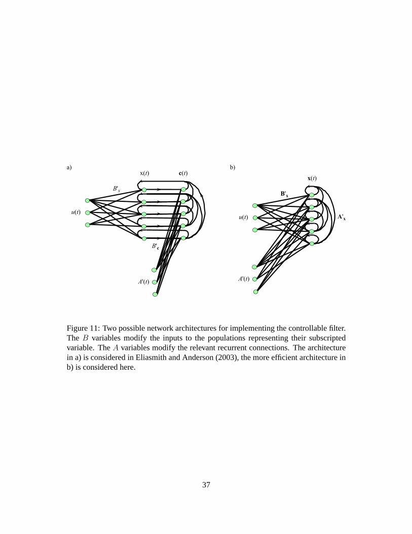
This means that our network must support multiplication at the higher level. The two

most obvious architectures for building this computation into the network are shown

in figure 11. Both architectures are implementations of the same high-level dynamics

equation

x(t) = h′(t) ∗ (A′(t)x(t) + τu(t)) (26)

which is no longer LTI, as it is clearly a time-varying system. Notably, while both

architectures demand multiplication at the higher level, this does not mean that there

needs to be multiplication between activities at the neural level. This is because, as

mentioned in section 2.2 and demonstrated in section 3.4, nonlinear functions can be

determined using only linear decoding weights.

As described in Eliasmith and Anderson (2003), the first architecture can be imple-

mented by constructing an intermediate representation of the vectorc = [A′, x] from

which the product is extracted using linear decoding. The result is then used as the

recurrent input to theaipopulation representingx. This circuit is successful, but per-

formance is improved by adopting the second architecture.

In the second architecture, the representation inai population is taken to be a 2D

representation ofx in which the first element is the integrated input and the second

36

u(t)

x(t)

B'x

A'(t)

c(t)

u(t)

x(t)

A'x

B'x

A'(t)

a) b)

B'c

Figure 11: Two possible network architectures for implementing the controllable filter.The B variables modify the inputs to the populations representing their subscriptedvariable. TheA variables modify the relevant recurrent connections. The architecturein a) is considered in Eliasmith and Anderson (2003), the more efficient architecture inb) is considered here.

37

element isA′. The product is extracted directly from this representation using linear

decoding and then used as feedback. This has the advantage over the first architecture

of not introducing extra delays and noise.

Specifically, letx = [x1, x2] (wherex1 = x andx2 = A′ in (26)). So, a more

accurate description of the higher-level dynamics equation for this system is

x = h′ ∗ (A′x + B′u) x1

x2

= h′ ∗

x2 0

0 0

x1

x2

+

τ 0

0 τ

u

A′

(27)

which makes the nonlinear nature of this implementation explicit. Notably, here the

desiredA′ is provided as input from a preceding population, as is the signal to be

integrated,u. To implement this system, we need to compute the transformation

p(t) =∑

i

ai(t)φpi ,

wherep(t) is the product of the elements ofx. Substituting this transformation into

(14) gives

aj = Gj

[αj

⟨h′ ∗ φj

[∑i

ai(t)φpi + B′∑

k

bk(t)φuk

]⟩+ J bias

j

]

= Gj

[∑i

ωijai(t) +∑k

ωkjbk(t) + J biasj

](28)

whereωij = αjφjφpi , ωkj = αjφjB

′φuk, and

ai(t) = h′ ∗ Gi

[αi

⟨x(t)φi

⟩+ J bias

i

].

38

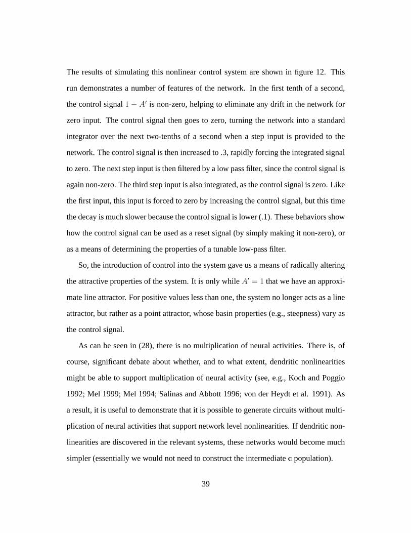
The results of simulating this nonlinear control system are shown in figure 12. This

run demonstrates a number of features of the network. In the first tenth of a second,

the control signal1 − A′ is non-zero, helping to eliminate any drift in the network for

zero input. The control signal then goes to zero, turning the network into a standard

integrator over the next two-tenths of a second when a step input is provided to the

network. The control signal is then increased to .3, rapidly forcing the integrated signal

to zero. The next step input is then filtered by a low pass filter, since the control signal is

again non-zero. The third step input is also integrated, as the control signal is zero. Like

the first input, this input is forced to zero by increasing the control signal, but this time

the decay is much slower because the control signal is lower (.1). These behaviors show

how the control signal can be used as a reset signal (by simply making it non-zero), or

as a means of determining the properties of a tunable low-pass filter.

So, the introduction of control into the system gave us a means of radically altering

the attractive properties of the system. It is only whileA′ = 1 that we have an approxi-

mate line attractor. For positive values less than one, the system no longer acts as a line

attractor, but rather as a point attractor, whose basin properties (e.g., steepness) vary as

the control signal.

As can be seen in (28), there is no multiplication of neural activities. There is, of

course, significant debate about whether, and to what extent, dendritic nonlinearities

might be able to support multiplication of neural activity (see, e.g., Koch and Poggio

1992; Mel 1999; Mel 1994; Salinas and Abbott 1996; von der Heydt et al. 1991). As

a result, it is useful to demonstrate that it is possible to generate circuits without multi-

plication of neural activities that support network level nonlinearities. If dendritic non-

linearities are discovered in the relevant systems, these networks would become much

simpler (essentially we would not need to construct the intermediatec population).

39

0 0.1 0.2 0.3 0.4 0.5 0.6 0.7 0.8 0.9 1

-0.2

0

0.2

0.4

0.6

0.8

1

Time (s)

Co

ntr

oll

ed F

ilte

r

0 0.1 0.2 0.3 0.4 0.5 0.6 0.7 0.8 0.9 1-1.5

-1

-0.5

0

0.5

1

1.5

Inp

ut

u(t)

1-A'(t)

x1(t)

x2(t)

a)

b)

Figure 12: The results of simulating the second architecture for a controllable filter ina spiking network of 2000 neurons under 10% noise. a) The input signals to the net-work. b) The high-level decoded response of the spiking neural network. The networkencodes both the integrated result and the control signal directly, to efficiently supportthe necessary nonlinearity. See text for a description of the behavior.

40

4.2 Controlling bump movement around a ring attractor

Of the two models presented in section 3.2, the role of control is most evident for the

head direction system. In order to be useful, the head direction system must be able

to update its current estimate of the heading of the animal given vestibular information

about changes in the animal’s heading. In terms of the ring attractor, this means that the

system must be able rotate the bump of activity around the ring in various directions

and at various speeds given simple left/right angular velocity commands.

To design a system that behaves in this way, we can first describe the problem in

the function spacex(ν) for a velocity commandδ/τ and then write this in terms of the

coefficientsx in the orthonormal Fourier space:

x(ν; t + τ) = x(ν + δ; t)

=∑m

xmeim(ν+δ)

=∑m

xmeimνeimδ.

So, rotation of the bump can be effected by applying the matrixEm = eimδ, whereδ

determines the speed of rotation. Written for real-valued functions,E becomes

E =

1 0 0 0

0 cos(mδ) sin(mδ) 0

0 − sin(mδ) cos(mδ)...

0 0 · · · ...

.

To derive the dynamics matrixA for the state equation (5), it is important to note that

41

E defines the new function att + τ , not just the change,δx. As well, we would like to

control the speed of rotation, so we can introduce a scalar on[−1, 1] that changes the

velocity of rotation, withδ defining the maximum velocity. Taking these considerations

into account, gives

A = C(t) (E− I)

whereC(t) is the left/right velocity command.6

As in section 4.1, we can include the time-varying scalar variableC(t) in the state

vectorx and perform the necessary multiplication by extracting a nonlinear function

that is the product of that element with the rest of the state vector. Doing so again

means that there is no need to multiply neural activities. Constructing a ring attractor

without multiplication is a problem that was only recently solved by Goodridge and

Touretzky (2000). That solution, however, is specific to a one-dimensional single bump

attractor, does not use spiking neurons, and does not include noise. As well, the so-

lution posits single left/right units that together project to every cell in the population,

necessitates the setting of normalization factors, and demands numerical experiments

to determine the appropriate value of a number of the parameters. In sum, the solu-

tion is somewhat non-biological and very specific to the problem being addressed. In

contrast, the solution I have presented here is subject to none of these concerns: it is

both biologically plausible and based on general principles. The behavior of the fully

6There is more subtlety than one might think to this equation. For values ofC(t) 6= 1, the systemdoes not behave as one might expect. For negative values, two bumps are created: one negative bump inthe direction opposite the desired direction of motion; and the other at the current bump location. Thisresults in the current bump being effectively ‘pushed away’ from the negative bump. For values less thanone, a proportionally scaled bump is created in the location as ifC(t) = 1, and a proportionally scaledbump is subtracted from the current position, resulting in proportionally scaled movement. There aretwo reasons that this equation works as expected. The first is that the movements are very small, so theresulting bumps in all cases are approximately Gaussian (though subtly bi-modal). The second is thatthe attractor dynamics built into the network ‘clean-up’ any non-Gaussianity of the resulting states. Theresult is a network that displays bumps moving in either direction proportional toC(t), as desired.

42

0

1

2

Tim

e (s)

πν-πLeft / Right

a) b)

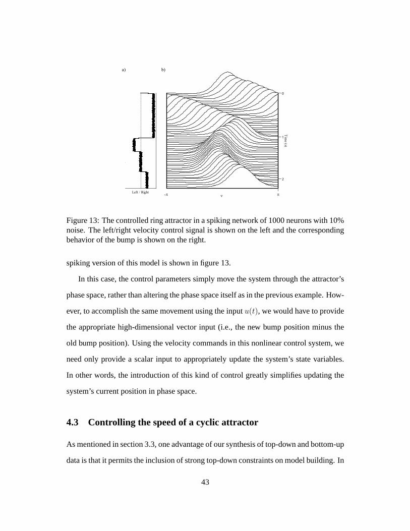
Figure 13: The controlled ring attractor in a spiking network of 1000 neurons with 10%noise. The left/right velocity control signal is shown on the left and the correspondingbehavior of the bump is shown on the right.

spiking version of this model is shown in figure 13.

In this case, the control parameters simply move the system through the attractor’s

phase space, rather than altering the phase space itself as in the previous example. How-

ever, to accomplish the same movement using the inputu(t), we would have to provide

the appropriate high-dimensional vector input (i.e., the new bump position minus the

old bump position). Using the velocity commands in this nonlinear control system, we

need only provide a scalar input to appropriately update the system’s state variables.

In other words, the introduction of this kind of control greatly simplifies updating the

system’s current position in phase space.

4.3 Controlling the speed of a cyclic attractor

As mentioned in section 3.3, one advantage of our synthesis of top-down and bottom-up

data is that it permits the inclusion of strong top-down constraints on model building. In

43

the context of lamprey locomotion, introducing control over swimming speed and guar-

anteeing stable oscillation to CPG-based models were problems that had to be tackled

separately, took much extra work, and resulted in solutions specific to this kind of net-

work (Marder et al. 1997). In contrast, stability, control, and other top-down constraints

can be included in the cyclic attractor model directly.

In this example, I consider control over swimming speed. Given the two previous

examples, we know that this kind of control can be characterized as the introduction

of non-linear or time-varying parameters into our state equations. For instance, we can

make the frequency termω in (23) a function of time. For simplicity, I will consider the

standard oscillator, although it is closely related to the swimming model as discussed

earlier (see Kuo and Eliasmith ress for an anatomically and physiologically plausible

model of zebrafish swimming with speed control).

To change the speed of an oscillator we need to implement:

x =

0 ω(t)

−ω(t) 0

x1

x2

+ Bu(t).

For this example, we can construct a nonlinear model, but unlike equation (27), we

do not have to increase the dimension of the state-space. Instead, we can increase the

dimension of the input space, so the third dimension carries the time-varying frequency

signal, giving

x =

0 u3(t)

−u3(t) 0

x1

x2

+ Bu(t). (29)

As before, this can be translated into a neural dynamics matrix using (7) and im-

plemented in a neural population using the methods analogous to those in section 4.1.

In fact, the architecture used for the neural implementation is the same despite the al-

44

0 0.5 1 1.5 2 2.5 3-1.5

-1

-0.5

0

0.5

1

1.5

Time (s)

x1

x2

ω

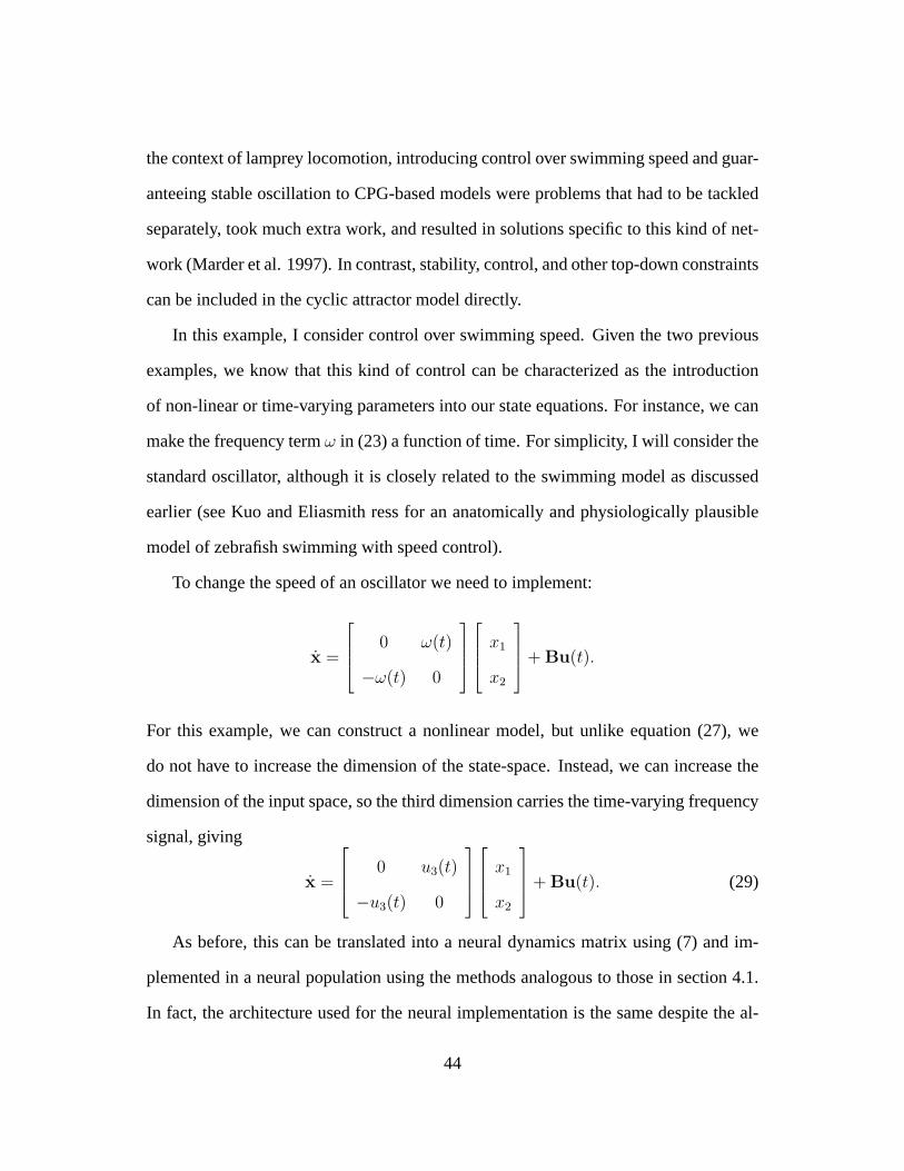
Figure 14: The controlled oscillator in a spiking network of 800 neurons with 10%noise. The control signal variesω, causing the oscillator to double its speed and thenslow down to the original speed.

ternate way of expressing the control system in (29). That is, in order to perform the

necessary multiplication, the dimensionality of the space encoded by the population

is increased by one. In this case, the extra dimension is assigned to the input vector

rather than the state vector. It should not be surprising, then, that we can successfully

implement a controlled cyclic attractor (see figure 14).

In this example, control is used to vary a property of the attractor, namely the period

of the orbit. Because the previous two examples are static attractors, this kind of control

does not apply to them. However, it should be clear that this example adds nothing new

theoretically. However, it helps to demonstrate that the methods introduced earlier ap-

ply broadly. Additionally, the introduction of this kind of control into a neural model of

swimming results in connectivity that matches the known anatomy (Kuo and Eliasmith

ress).

45

4.4 Moving between chaotic, cyclic, and point attractors

Both Skarda and Freeman (1987) and Kelso and Fuchs (1995) have suggested that being

in a chaotic attractor may help to improve the speed of response of a neural system to

various perturbations. In other words, they suggest that if chaotic dynamics are to be

useful to a neural system it must be possible to move into and out of the chaotic regime.

Conveniently, the bifurcations and attractor structures in the Lorenz equations (24) are

well-characterized, making them ideal for introducing the kind of control needed to

enter and exit the chaotic attractor.

For instance, changing theb parameter over the range[1, 300] causes the system

to exhibit point, chaotic and cyclic attractors. So, constructing a neural control sys-

tem with an architecture analogous to that of the controlled integrator discussed earlier

would allow us to move the system between these kinds of states.

However, an implementational difficulty arises. As suggested by figure 10, the

mean of thex3variable is roughly equal tob. Thus, for largely varying values ofb, the

neural system will have to represent a large range of values, necessitating a very wide

dynamic range with a good signal to noise ratio. This can be achieved with enough

neurons, but it is more efficient to re-write the Lorenz equations to preserve the dynam-

ics, but eliminate the scaling problem. To do so, we can simply subtract and addb as

appropriate to remove the scaling effect. This gives

x1

x2

x3

=

a(x2 − x1)

bx1 − x2 − x1(x3 + b)

x1x2 − c(x3 + b) − b

46

=

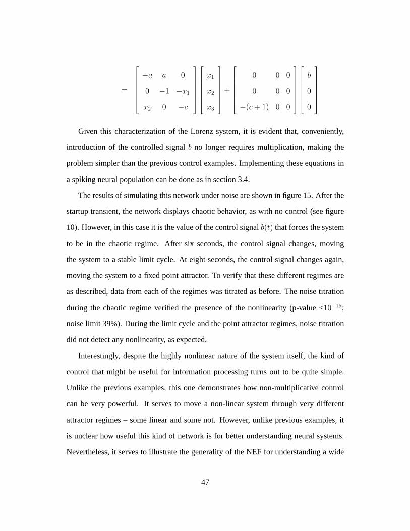
−a a 0

0 −1 −x1

x2 0 −c

x1

x2

x3

+

0 0 0

0 0 0

−(c + 1) 0 0

b

0

0

Given this characterization of the Lorenz system, it is evident that, conveniently,

introduction of the controlled signalb no longer requires multiplication, making the

problem simpler than the previous control examples. Implementing these equations in

a spiking neural population can be done as in section 3.4.

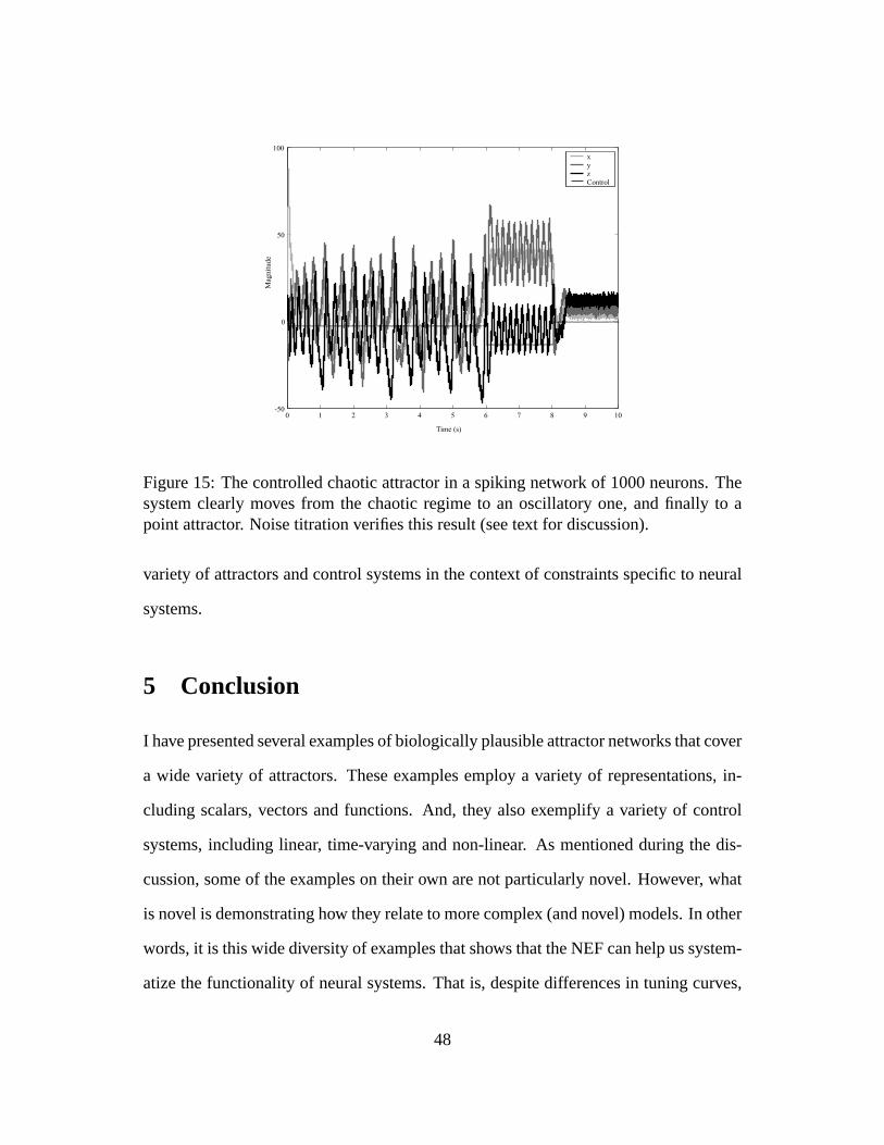
The results of simulating this network under noise are shown in figure 15. After the

startup transient, the network displays chaotic behavior, as with no control (see figure

10). However, in this case it is the value of the control signalb(t) that forces the system

to be in the chaotic regime. After six seconds, the control signal changes, moving

the system to a stable limit cycle. At eight seconds, the control signal changes again,

moving the system to a fixed point attractor. To verify that these different regimes are

as described, data from each of the regimes was titrated as before. The noise titration

during the chaotic regime verified the presence of the nonlinearity (p-value <10−15;

noise limit 39%). During the limit cycle and the point attractor regimes, noise titration

did not detect any nonlinearity, as expected.

Interestingly, despite the highly nonlinear nature of the system itself, the kind of

control that might be useful for information processing turns out to be quite simple.

Unlike the previous examples, this one demonstrates how non-multiplicative control

can be very powerful. It serves to move a non-linear system through very different

attractor regimes – some linear and some not. However, unlike previous examples, it

is unclear how useful this kind of network is for better understanding neural systems.

Nevertheless, it serves to illustrate the generality of the NEF for understanding a wide

47

0 1 2 3 4 5 6 7 8 9 10-50

0

50

100

Time (s)

Mag

nit

ude

x

y

z

Control

Figure 15: The controlled chaotic attractor in a spiking network of 1000 neurons. Thesystem clearly moves from the chaotic regime to an oscillatory one, and finally to apoint attractor. Noise titration verifies this result (see text for discussion).

variety of attractors and control systems in the context of constraints specific to neural

systems.

5 Conclusion

I have presented several examples of biologically plausible attractor networks that cover

a wide variety of attractors. These examples employ a variety of representations, in-

cluding scalars, vectors and functions. And, they also exemplify a variety of control

systems, including linear, time-varying and non-linear. As mentioned during the dis-

cussion, some of the examples on their own are not particularly novel. However, what

is novel is demonstrating how they relate to more complex (and novel) models. In other

words, it is this wide diversity of examples that shows that the NEF can help us system-

atize the functionality of neural systems. That is, despite differences in tuning curves,

48

kinds of representation, neural response properties, intrinsic dynamics, and so on, it is

possible to classify various networks as variations on themes of integration, filtering,

oscillation, etc. all of which can be derived from simple, general principles. Further-

more, characterizing high-level dynamics, and how lower-level properties affect those

dynamics, can provide a window into the purpose of neural subsystems. Compiling

this knowledge should aid in more quickly understanding the likely functions of larger,

more complex, and less familiar systems.

This kind of systematization can be useful in a number of ways. For one, it suggests

that perhaps the kinds of networks I have described here can serve as functional parts

of larger networks – networks which we can construct using these same methods. One

example of this is presented in Eliasmith et al. (2002), where an integrator is one of

nine subnetworks used to estimate the true translational velocity of an animal given

the responses of semicircular canals and otoliths to a variety of acceleration profiles.

So, while I have used the NEF here to construct a specific class of networks, the same

methods are more broadly applicable.

A second benefit of systematization, as mentioned earlier, is that it supports the

transfer of knowledge and analyses regarding well-understood neural systems to lesser-

understood ones. So, for instance, understanding a useful control structure for the

ring attractor suggests a useful control structure for path integration, a lesser-studied

and more complex neural system (Conklin and Eliasmith 2004). More generally, if

we can see the close relation between two high-level descriptions of different neural

systems (e.g., working memory and the neural integrator, or path integration and the

head-direction system), what we have learned about one may often be ‘translated’ into

implications for the other. This can greatly speed up the development of novel mod-

els and focus our attention on the important characteristics of new systems (be they

49

similarities to, or differences from, other known systems).

Finally, by being able to provide the high-level characterizations of neural systems

upon which such systematization depends, we can carefully introduce new complexities

into existing models. For instance, the recent surge of interest in the observed dynamics

of working memory (Miller et al. 2003; Romo et al. 1999; Brody et al. 2003), can

be captured by simple extensions of the models described earlier (Singh and Eliasmith

2004). Again, this can greatly aid the construction of novel models – models which may

be able to address more complicated phenomena than otherwise possible (Eliasmith

et al. (2004) presents a neuron-level model of a well-studied deductive inference task

(the Wason card selection task) with 14 subsystems).

So, while this discussion has focused on characterizing a class of networks that is

clearly important for understanding neural systems, the methods underlying this ap-

proach have much broader application. That is, they can help us begin to better under-

stand the general control and routing of information through the brain in a way respon-

sible to neural constraints. With continuing improvement in experimental techniques

for examining large-scale networks, theoretical tools for understanding networks on a

the same scale become essential. I would like to suggest that the examples provided

here hint that the NEF may be a useful attempt at beginning to develop such tools.

Acknowledgments

I would like to express special thanks to John Conklin, Charles H. Anderson and

Valentin Zhigulin and for helpful discussions. I would like to further thank John Con-

klin for generating the figures related to the ring attractor. The noise titration code for

detecting chaos was graciously provided by Chi-Sang Poon. This work is supported

50

by grants from the National Science and Engineering Research Council of Canada, the

Canadian Foundation for Innovation, the Ontario Innovation Trust and the McDonnell

Project in Philosophy and the Neurosciences.

Appendix A

Consider determining the optimal linear decodersφi in (3) under noise (see also Salinas

and Abbott 1994). To include noise, we introduce the noise termηi which is drawn from

a Gaussian, independent, identically distributed, zero mean distribution. The noise is

added to the neuron activityai resulting in a decoding of

x =N∑

i=1

(ai(x) + ηi) φi. (30)

To find the least squares optimalφi, we construct and minimize the mean square error,

averaging over the expected noise and the vectorx:

E =1

2

⟨[x−

N∑i=1

(ai(x) + ηi) φi

]2⟩x,η

=1

2

⟨[x−

(N∑

i=1

ai(x)φi −N∑

i=1

ηiφi

)]2⟩x,η

(31)

where〈·〉xindicates integration over the range ofx. Because the noise is independent

on each neuron, the noise averages out except wheni = j. So, the average of theηiηj

noise is equal to the varianceσ2 of the noise on the neurons. Thus, the error with noise

becomes

E =1

2

⟨[x−

N∑i=1

ai(x)φi

]2⟩x

+1

2σ2

N∑i=1

φ2i . (32)

51

Taking the derivative of the error gives

δE

δφi

= −1

2

⟨2

x−N∑j

aj(x)φj

ai(x)

⟩x

+ σ2φjδij

= −〈ai(x)x〉x +

⟨N∑j

ai(x)aj(x)φj

⟩x

+ σ2φjδij. (33)

Setting the derivative to zero gives

〈ai(x)x〉x =N∑j

(〈ai(x)aj(x)〉x + σ2δij

)φj (34)

or, in matrix form,

Υ = Γφ.

The decoding vectorsφiare given by

φ = Γ−1Υ

where

Γij = 〈ai(x)aj(x)〉x + σ2δij

Υi = 〈xai(x)〉x .

Notice that theΓ matrix will be non-singular because of the noise term on the diagonal.

Much of the power of this framework comes from the simple observation that this

same procedure can be followed to find the optimal linear decodersφf(x) for some

52

arbitrary functionf(x). The error to be minimized then becomes

E =1

2

⟨[f(x) −

N∑i=1

(ai(x) + ηi) φf(x)i

]2⟩x,η

.

The minimization is analogous, with only a differing result forΥ:

Υi = 〈f(x)ai(x)〉x .

This extension provides the impetus for analyses of the functions that are possible

to compute given a specific neural population (i.e., set ofai(x) curves). While not

reproduced here, these analyses demonstrate that polynomial nonlinearities are well-

supported by neurons with broad tuning curves (Eliasmith and Anderson 2003, chp. 7).

Thus we can be assured that computing products, as done in the networks presented

here, can be done with sufficient accuracy. It is this ability that makes the inclusion of

both nonlinear and time-varying control systems within this framework a possibility.

References

Amit, D. J. (1989).Modeling brain function: The world of attractor neural networks.

New York, NY: Cambridge University Press.

Askay, E., G. Gamkrelidze, H. S. Seung, R. Baker, and D. Tank (2001). In vivo in-

tracellular recording and perturbation of persistent activity in a neural integrator.

Nature Neuroscience 4, 184–193.

Biswal, B. and C. Dasgupta (2002). Neural network model for apparent deterministic

chaos in spontaneously bursting hippocampal slices.Physical Review Letters 88,

53

088102.

Bradley, E. (1995). Autonomous exploration and control of chaotic systems.Cyber-

netics and Systems 26, 299–319.

Brody, C. D., R. Romo, and A. Kepecs (2003). Basic mechanisms for graded persis-

tent activity: discrete attractors, continuous attractors, and dynamic representa-

tions.Current Opinion in Neurobiology 13, 204–211.

Conklin, J. and C. Eliasmith (2004). A controlled attractor network model of path

integration in the rat.unpublished.

Eliasmith, C. and C. H. Anderson (2000). Rethinking central pattern generators: A

general approach.Neurocomputing 32, 735–740.

Eliasmith, C. and C. H. Anderson (2003).Neural engineering: Computation, rep-

resentation, and dynamics in neurobiological systems. Cambridge, MA: MIT

Press.

Eliasmith, C., J. Conklin, and R. Singh (2004, March 24–28). A neurobiological

simulation of deductive reasoning. InComputational and Systems Neuroscience

2004, Cold Spring Harbour, NY.

Eliasmith, C., M. B. Westover, and C. H. Anderson (2002). A general framework for

neurobiological modeling: An application to the vestibular system.Neurocom-

puting 46, 1071–1076.

Fukushima, K., C. R. S. Kaneko, and A. F. Fuchs (1992). The neuronal substrate of

integration in the oculomotor system.Progress in Neurobiology 39, 609–639.

Fuster, J. M. (2001). The prefrontal cortex – an update: time is of the essence.Neu-

ron 30, 319–333.

54

Goodridge, J. P. and D. S. Touretzky (2000). Modeling attractor deformation in the

rodent head-direction system.Journal of Neurophysiology 83, 3402–3410.

Grillner, S., P. Wallén, L. Brodin, and A. Lansner (1991). The neuronal network

generating locomotor behavior in lamprey: Circuitry, transmitters, membrane

properties, and simulation.Annual Review of Neuroscience 14, 169–199.

Hansel, D. and H. Sompolinsky (1998). Modeling feature selectivity in local cor-

tical circuits. In C. Koch and I. Segev (Eds.),Methods in neuronal modeling.

Cambridge, MA: MIT Press.

Hebb, D. O. (1949).The organization of behavior. New York, NY: Wiley.

Hopfield, J. J. (1982). Neural networks and physical systems with emergent col-

lective computational abilities.Proceedings of the National Academy of Sci-

ences 79, 2554–2558.

Kelso, J. A. S. and A. Fuchs (1995). Self-organizing dynamics of the human brain:

Critical instabilities and silnikov chaos.Chaos 5, 64–69.

Koch, C. and T. Poggio (1992). Multiplying with synapses and neurons. In

T. McKenna, J. Davis, and S. F. Zornetzer (Eds.),Single neuron computation.

Boston, MA: Academic Press.

Kopell, N. and G. B. Ermentrout (1988). Coupled oscillators and the design of cen-

tral pattern generators.Mathematical Biosciences 90, 87–109.

Kuo, D. and C. Eliasmith (in press). Understanding interactions between networks

controlling distinct behaviors: Escape and swimming in larval zebrafish.Neuro-

computing.

Lai, Y.-C., M. A. Harrison, M. G. Frei, , and I. Osorio (2003). Inability of lyapunov

55

exponents to predict epileptic seizures.Physical Review Letters 91, 068012.

Laing, C. R. and C. C. Chow (2001). Stationary bumps in networks of spiking neu-

rons.Neural Computation 13, 1473–1494.

Manira, A. E., J. Tegnér, and S. Grillner (1994). Calcium-dependent potassium chan-

nels play a critical role for burst termination in the locomotor network in lamprey.

Journal of Neurophysiology 4, 1852–1861.

Marder, E., N. Kopell, and K. Sigvardt (1997). How computation aids in understand-

ing biological networks. In P. Stein, S. Grillner, A. Selverston, and D. Stuart

(Eds.),Neurons, networks, and motor behavior. Cambridge, MA: MIT Press.

Matsugu, M., J. Duffin, and C. Poon (1998). Entrainment, instability, quasi-

periodicity, and chaos in a compound neural oscillator.Journal of Computational

Neuroscience 5, 35–51.

Mel, B. (1994). Information processing in dendritic trees.Neural Computation 6,

1031–1085.

Mel, B. (1999). Why have dendrites? a computational perspective. In G. Stuart,

N. Spruston, and M. Häusser (Eds.),Dendrites. New York, NY: Oxford Univer-

sity Press.

Miller, P., C. Brody, R. Romo, and X.-J. Wang (2003). A recurrent network model

of somatosensory parametric working memory in the prefrontal cortex.Cerebral

Cortex 13, 1208–1218.

Platt, M. L. and G. W. Glimcher (1998). Response fields of intraparietal neurons

quantified with multiple saccadic targets.Experimental Brain Research 121, 65–

75.

56

Poon, C.-S. and M. Barahona (2001). Titration of chaos with added noise.Proceed-

ings of the National Academy of Science 98, 7107–7112.

Pouget, A., K. Zhang, S. Deneve, and P. E. Latham (1998). Statistically efficient

estimation using population coding.Neural Computation 10, 373–401.

Rainer, G. and E. K. Miller (2002). Timecourse of object-related neural activity in

the primate prefrontal cortex during a short-term memory task.European Journal

of Neuroscience 15, 1244–1254.

Redish, A. D. (1999).Beyond the cognitive map. Cambridge, MA: MIT Press.

Rieke, F., D. Warland, R. R. de Ruyter van Steveninick, and W. Bialek (1997).

Spikes: Exploring the neural code. Cambridge, MA: MIT Press.

Romo, R., C. D. Brody, A. Hernández, and L. Lemus (1999). Neuronal correlates of

parametric working memory in the prefrontal cortex.Nature 399, 470–473.

Salinas, E. and L. F. Abbott (1994). Vector reconstruction from firing rates.Journal

of Computational Neuroscience 1, 89–107.

Salinas, E. and L. F. Abbott (1996). A model of multiplicative neural responses

in parietal cortex.Proceedings of the National Academy of Sciences USA 93,

11956–11961.

Selverston, A. I. (1980). Are central pattern generators understandable?Behavioral

and Brain Sciences 3, 535–571.

Sereno, A. B. and J. H. R. Maunsell (1998). Shape selectivity in primate lateral

intraparietal cortex.Nature 395, 500–503.

Seung, H. S. (1996). How the brain keeps the eyes still.Proceedings of the National

Academy of Sciences, USA 93, 13339–13344.

57

Seung, H. S., D. Lee, B. Reis, and D. Tank (2000). Stability of the memory of eye

position in a recurrent network of conductance-based model neurons.Neuron 26,

259–271.

Shadlen, N. N. and W. T. Newsome (2001). Neural basis of a perceptual decision

in the parietal cortex (area lip) of the rhesus monkey.Journal of Neurophysiol-

ogy 86, 1916–1936.

Singh, R. and C. Eliasmith (2004, March 24–28). A dynamic model of working

memory in the pfc during a somatosensory discrimination task. InComputational

and Systems Neuroscience 2004, Cold Spring Harbour, NY.

Skarda, C. A. and W. J. Freeman (1987). How brains make chaos in order to make

sense of the world.Behavioral and Brain Sciences 10, 161–195.

Snyder, L. H., A. P. Batista, and R. A. Andersen (1997). Coding of intention in the

posterior parietal cortex.Nature 386, 167–170.

Touretzky, D. S. and A. D. Redish (1996). Theory of rodent navigation based on

interacting representations of space.Hippocampus 6, 247–270.

von der Heydt, R., E. Peterhans, and M. Dursteler (1991). Grating cells in monkey

visual cortex: Coding texture? In B. Blum (Ed.),Channels in the visual nervous

system: Neurophysiology, psychophysics, and models. London: Freund.

Zhang, K. (1996). Representation of spatial orientation by the intrinsic dynamics of

the head-direction cell ensemble: A theory.Journal of Neuroscience 16, 2112–

2126.

58