A Unified Analysis of Structured

Sonar-terrain Data using Bayesian

Functional Mixed Models

Hongxiao Zhu

Department of Statistics, Virginia Tech, Blacksburg, VA 24061Philip Caspers

Department of Mechanical Engineering, Virginia Tech, Blacksburg, VA 24061Jeffrey S. Morris

The University of Texas M.D. Anderson Cancer Center,Houston, TX 77230Xiaowei Wu

Department of Statistics, Virginia Tech, Blacksburg, VA 24061and

Rolf Muller

Department of Mechanical Engineering, Virginia Tech, Blacksburg, VA 24061

Abstract

Sonar emits pulses of sound and uses the reflected echoes to gain information abouttarget objects. It offers a low cost, complementary sensing modality for small roboticplatforms. While existing analytical approaches often assume independence acrossechoes, real sonar data can have more complicated structures due to device setupor experimental design. In this paper, we consider sonar echo data collected frommultiple terrain substrates with a dual-channel sonar head. Our goals are to identifythe differential sonar responses to terrains and study the effectiveness of this dual-channel design in discriminating targets. We describe a unified analytical frameworkthat achieves these goals rigorously, simultaneously, and automatically. The analysiswas done by treating the echo envelope signals as functional responses and the ter-rain/channel information as covariates in a functional regression setting. We adoptfunctional mixed models that facilitate the estimation of terrain and channel effectswhile capturing the complex hierarchical structure in data. This unified analyticalframework incorporates both Gaussian models and robust models. We fit the modelsusing a full Bayesian approach, which enables us to perform multiple inferential tasksunder the same modeling framework, including selecting models, estimating the ef-fects of interest, identifying significant local regions, discriminating terrain types, anddescribing the discriminatory power of local regions. Our analysis of the sonar-terrain

1

data identifies time regions that reflect differential sonar responses to terrains. Thediscriminant analysis suggests that a multi- or dual-channel design achieves targetidentification performance comparable with or better than a single-channel design.

Keywords: Echo data; Acoustic data; Functional regression; Bayesian methods; Mixedeffects model; Discriminant analysis; Wavelets.

technometrics tex template (do not remove)

2

1 Introduction

Sonar (Sound Navigation and Ranging) is a technique that uses sound propagation

to detect, localize, and identify objects for purposes such as navigation. An active sonar

system transmits acoustic waves with a known time waveform and receives the echoes

reflected by obstacles. During propagation and reflection, the transmitted waves will be

transformed due to physical effects such as propagation delays, frequency-dependent atten-

uation, frequency-shifts, and the addition of noise. These modifications are captured in the

received echoes and can be used to infer the characteristics of the targets (Le Chevalier,

2002) and the propagation channel. In complex, natural environments, an echo signal of-

ten consists of reflected waveforms from numerous scatterers that are distributed in space

(e.g., tree leaves, rocks), thus can be non-stationary, non-Gaussian, and highly stochastic

(Muller and Kuc, 2000; Yovel et al., 2008). This makes identification and navigation with

over-simplified physical models unrealistic. Statistical approaches are therefore highly de-

sirable in order to study sonar responses to targets, and extract useful information about

the environment (Robertson, 1996; Vicente Martinez Diaz, n.d.).

In a study that investigates echoes in natural environments, a sonar device was used to

collect echoes from three types of terrain substrates: grass, sand, and a simulated tropical

rainforest floor. The experiment was carried out by collecting echoes over multiple locations

within each terrain substrate, producing multiple sonar “footprints”. Each footprint con-

tains a group of repeatedly measured echoes from a fixed location. Additionally, the sonar

device has two built-in channels, each resulting in echoes with a different carrier frequency

(the center frequency of the emitted waveforms). Therefore each echo measurement gives

two echoes, one from each channel. This produces an acoustic dataset consisting of echo

signals measured from two channels, multiple footprints, and over three terrain substrates.

Based on this data, several scientific questions need to be investigated: (1) Can we identify

the “echo signatures” of different terrain substrates, i.e., regions of the echoes that are dif-

ferent across terrains? (2) What are the systematic differences between the two channels?

(3) Does the dual-channel design result in better performance than a single channel design

in terms of identifying terrain substrates? Addressing these questions requires rigorous

statistical analysis that not only characterizes the relationships between the echo data and

3

the variables of interest, but also takes into account the complex data structures such as

the hierarchical structure caused by measuring echoes by footprints.

In ultrasonic sensing, echolocation, and related fields, researchers have analyzed echo

data to study their acoustic properties (Muller and Kuc, 2000), their relationships with

targets (Phillip and Kristiansen, 2006; Yovel et al., 2009), and their variations across mul-

tiple measurements (Fahner et al., 2004). Most of these analyses are based on reducing the

dimension of the echo signals by selecting features subjectively (Muller and Kuc, 2000; Kuc,

2001; Muller, 2003), or applying dimension reduction methods such as principal component

analysis (Yovel et al., 2008). The features extracted are then used for different modeling

purposes including classification (Bozma, 1994; Kleeman and Kuc, 1995; Kuc, 2001; Muller,

2003; Von Helversen, 2004; Yovel et al., 2008), clustering (Reyes Reyes et al., 2015), and

analysis of variance (ANOVA) (Fahner et al., 2004).

While existing approaches were successful in solving a variety of problems, they may

be inadequate or non-applicable to our analysis because of the following reasons. First,

most existing approaches rely on pre-specified features extracted from the echo data, hence

could miss important information not captured by these features. Second, most analyses

assume independence across echo measurements and ignore important data structures such

as clusters caused by footprints. Third, to our knowledge, no existing analyses can be used

to identify local time regions of the echoes with differential responses to different targets.

Fourth, while Muller and Kuc (2000) have pointed out that echoes from natural targets

(e.g., foliages) could be non-Gaussian and non-stationary, no existing analyses explicitly

take into account the non-Gaussianity and non-stationarity of the echo time series. Finally,

existing approaches that study echo variations across multiple measurements, such as the

ANOVA analysis in Fahner et al. (2004), are not suitable for terrain classification. Therefore

to answer our questions, one needs to formulate separate models for the same dataset, which

is inefficient and may cause difficulty in interpreting results.

To address these issues, we adopt a functional regression approach (Ramsay and Silver-

man, 1997; Morris, 2015) treating the envelopes of the echoes as functional responses and

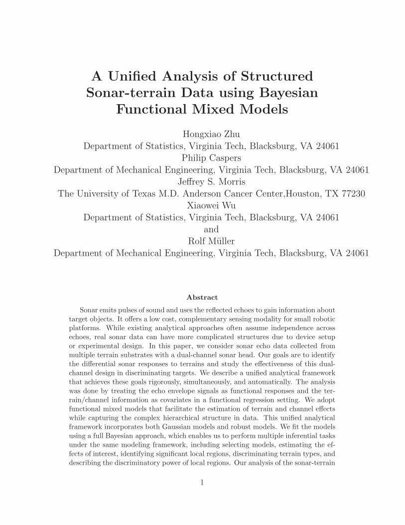
the different types of terrains and channels as covariates. The envelope of an echo signal

is the boundary curve within which all amplitude values of the signal are contained, as

4

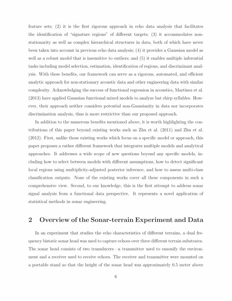
seen from the black curves in Figure 1. Intuitively, the envelope can be considered as a

“wrapper” that encloses a fast oscillating signal, capturing the low frequency fluctuations.

The envelopes retain the target-specific information through capturing lower frequency am-

5 5.2 5.4 5.6 5.8 6 6.2 6.4 6.6 6.8

−0.5

0

0.5

time (ms)

ampl

itude

The Envelope of a Sonar Echo Waveform

upper envelope →

lower envelope →

Figure 1: The upper and lower envelopes of an echo waveform.

plitude variations while removing the carrier frequency in echo, which makes it an ideal

representation for echo data. In the sonar echo data, since the upper and the lower en-

velopes are always symmetric, we only consider the upper envelopes in our analysis.

We account for the intricate structure of the data using functional mixed models

(FMMs). Guo (2002) appears to be the first to outline the mixed model framework for

functional data. Morris and Carroll (2006) proposed a Gaussian process FMM under the

Bayesian setup, and their approach was further extended by Zhu et al. (2011) to incorporate

data with non-Gaussian behaviors. Despite its success in modeling various data structures

(Morris et al., 2008; Davidson, 2009; Morris et al., 2011; Lancia et al., 2015), FMM has

been primarily used to characterize the effects of covariates. It remains unclear how the

FMM framework can be used to tackle all inferential challenges posed by the sonar-terrain

analysis. In this paper, we provide an analytical approach that addresses all relevant infer-

ential problems in sonar-terrain analysis rigorously, simultaneously, and automatically in a

single unified framework. We adopt a fully Bayesian approach that provides convenient es-

timation of the terrain and channel effects, facilitates multiplicity-adjusted inference to flag

interesting local regions, and naturally enables model selection and discriminant analysis.

Comparing with conventional approaches, the proposed framework brings several ad-

vantages to sonar analysis: (1) it models the entire envelope signal directly, providing a

statistically principled alternative to existing analytical approaches based on pre-specified

5

feature sets; (2) it is the first rigorous approach in echo data analysis that facilitates

the identification of “signature regions” of different targets; (3) it accommodates non-

stationarity as well as complex hierarchical structures in data, both of which have never

been taken into account in previous echo data analysis; (4) it provides a Gaussian model as

well as a robust model that is insensitive to outliers; and (5) it enables multiple inferential

tasks including model selection, estimation, identification of regions, and discriminant anal-

ysis. With these benefits, our framework can serve as a rigorous, automated, and efficient

analytic approach for non-stationary acoustic data and other engineering data with similar

complexity. Acknowledging the success of functional regression in acoustics, Martinez et al.

(2013) have applied Gaussian functional mixed models to analyze bat chirp syllables. How-

ever, their approach neither considers potential non-Gaussianity in data nor incorporates

discrimination analysis, thus is more restrictive than our proposed approach.

In addition to the numerous benefits mentioned above, it is worth highlighting the con-

tributions of this paper beyond existing works such as Zhu et al. (2011) and Zhu et al.

(2012). First, unlike those existing works which focus on a specific model or approach, this

paper proposes a rather different framework that integrates multiple models and analytical

approaches. It addresses a wide scope of new questions beyond any specific models, in-

cluding how to select between models with different assumptions, how to detect significant

local regions using multiplicity-adjusted posterior inference, and how to assess multi-class

classification outputs. None of the existing works cover all these components in such a

comprehensive view. Second, to our knowledge, this is the first attempt to address sonar

signal analysis from a functional data perspective. It represents a novel application of

statistical methods in sonar engineering.

2 Overview of the Sonar-terrain Experiment and Data

In an experiment that studies the echo characteristics of different terrains, a dual fre-

quency bistatic sonar head was used to capture echoes over three different terrain substrates.

The sonar head consists of two transducers—a transmitter used to ensonify the environ-

ment and a receiver used to receive echoes. The receiver and transmitter were mounted on

a portable stand so that the height of the sonar head was approximately 0.5 meter above

6

the ground. The sonar head was adjusted to face the terrain substrate with a fixed angle,

so that during each measurement, a specific patch (a footprint) of the substrate was en-

sonified and echoes were collected. Two transmitting/receiving channels were used in the

transducers to ensonify the environment and capture the returned echoes, with the fun-

damental (central) carrier frequencies 25 kHz and 40 kHz respectively. The dual-channel

design brings two potential advantages: (i) it collects data more efficiently—collecting the

same amount of data only requires half of the time than a signal-channel sonar; (ii) the

two channels allow more diverse sonar responses, leading to potentially more robust target

identification performance. More details of the experimental setup are provided in Sup-

plementary Material. In this experiment, the height of the sonar head (0.5 m) was set to

represent the situation of a small autonomous vehicle, either airborne or terrestrial. For

example, such sonar head can be mounted on platforms such as the Pioneer 3-DX ground

robot or the DJI S900 hexacopter. Such vehicles are often operated in close proximity to

terrain.

Echoes were collected over three different terrain substrates: grass, rainforest, and

sand. The measurements were taken by footprints. At each footprint, a set of echoes were

collected over a patch of the substrate; the sonar head was then reoriented or moved a few

meters away to collect another set of echoes. The total area of an experimental substrate

determines how many unique footprints we can measure. For grass and sand, a total of 40

footprints were taken, whereas for the rainforest substrate, only 29 footprints were taken

due to the smaller area of the experimental field. Each footprint contains 40 echoes, 20

from each channel. This gives a total of 4360 echoes, with half of the measurements from

the channel with carrier frequency 25 kHz and half from 40 kHz.

A number of preprocessing steps have been performed based on the raw echo signals,

including: (1) truncation of the recorded ensonifying impulse and the echo tails beyond 3

meter, (2) bandpass filter around each center frequency to remove noise, and (3) envelope

extraction via the Hilbert transform. The ensonifying impulse is the impulse caused by the

transmitted waveform hence does not contain substrate information. Echo tails correspond-

ing to a distance beyond the substrate range contain no information about the substrate

thus can also be removed. The envelope of the echo signal captures the amplitude variation

7

which is believed to be mainly influenced by the target properties, hence are extracted and

treated as the final data to be analyzed. Since the echo signals are symmetric about zero,

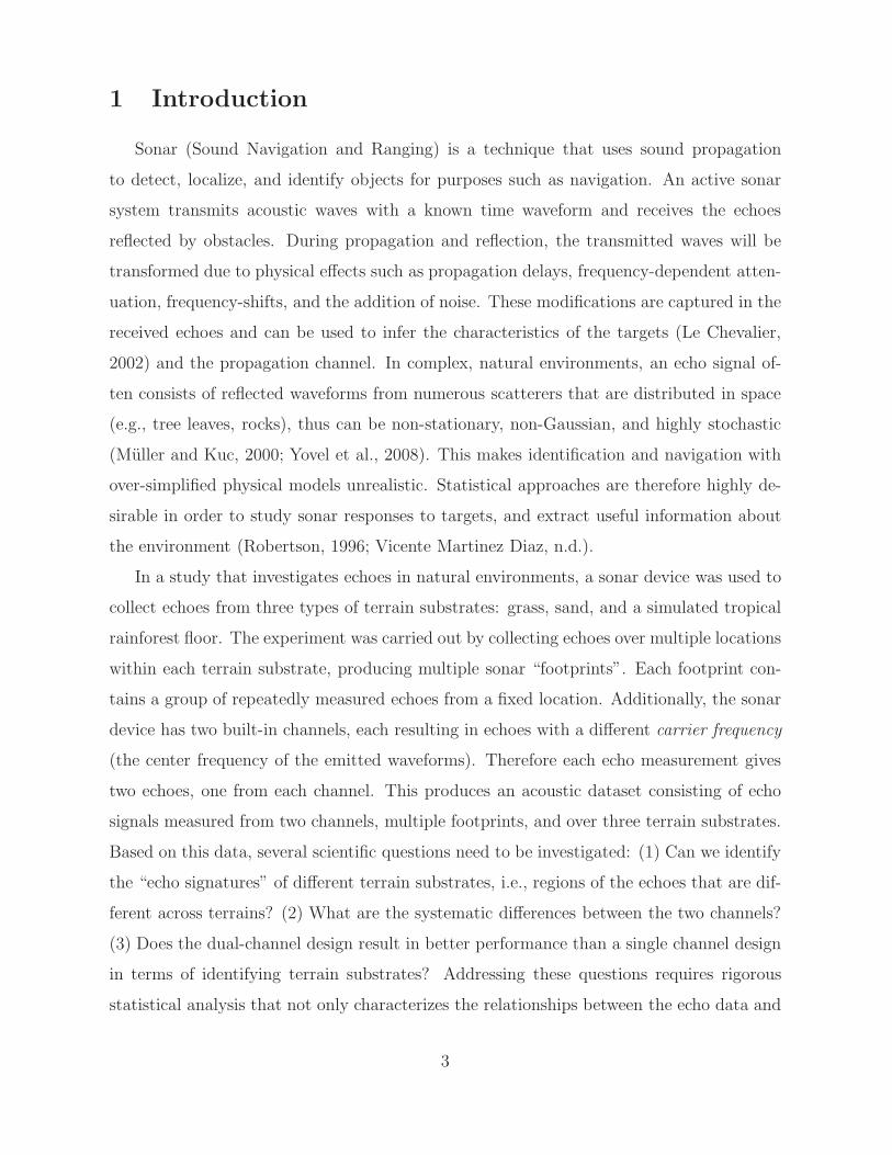
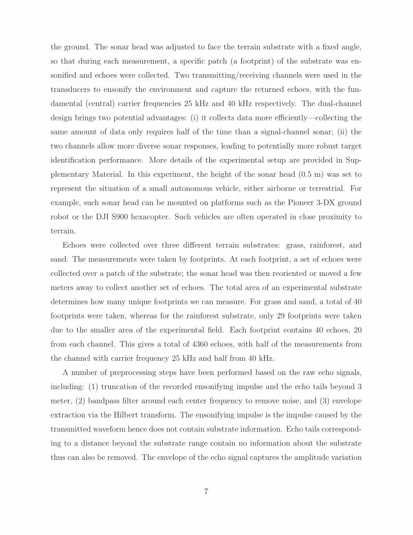
only the upper envelopes were considered. Figure 2 shows a preprocessed echo signal (in

5 10 15 20−2

0

2Grass, chan=25khz

5 10 15 20−2

0

2Grass, chan=40khz

time (ms)

5 10 15 20

−1

0

1

Rainforest, chan=25khz

5 10 15 20

−1

0

1

Rainforest, chan=40khz

time (ms)

5 10 15 20

−1

0

1

Sand, chan=25khz

5 10 15 20

−1

0

1

Sand, chan=40khz

time (ms)

Figure 2: Preprocessed echoes (in blue) and the extracted envelopes (in red).

gray color) superimposed with the extracted envelope (in black color) for two channels (row

1 vs. row 2) and the three terrain substrates (columns 1-3). Note that for each terrain,

the signals from the two channels shown in the upper and lower rows in Figure 2 are a pair

of echoes collected from the same measurement at the same footprint. We will treat the

envelope signals as functional data and study their characteristics and their relationships

with the terrain types and channels.

3 The Functional Mixed Models

In this section, we describe FMM for the sonar-terrain data and briefly review two

model setups: the Gaussian functional mixed model (Gfmm) and the robust functional

mixed model (Rfmm). Note that both Gfmm and Rfmm are not methodologically new.

The general methods have been proposed by Morris and Carroll (2006) and Zhu et al.

(2011); extensions and applications can be found in Zhu et al. (2012), Martinez et al.

(2013), Lee and Morris (2016), among others. The purpose of this section is not to propose

a brand new model, but to outline the FMMs in the context of sonar-terrain data analysis,

with the goal of integrating them in the unified analytical framework in Section 4.

8

Suppose that a total of M footprints are measured on A terrain substrates using two

channels. Let Yij(t) represent the envelope j in footprint i evaluated at time t, where

i = 1, . . . ,M , j = 1, . . . , mi, and t ∈ T . Let vija = 1 if Yij(t) is obtained on terrain type a,

a = 1, . . . , A and 0 otherwise; let xij = 1 if Yij(t) is measured by channel 1, and xij = −1

if measured by channel 2. We associate the envelopes with the terrain type and channel

information through a general functional mixed model (FMM):

Yij(t) =

A∑

a=1

vijaGa(t) + xijB(t) + Ui(t) + Eij(t), (1)

where Ga(t) represents the mean effect for terrain type a, B(t) represents the effect of two

channels, Ui(t) is a mean-zero random effect function capturing the footprint variability,

and Eij(t) is a mean-zero residual error function capturing intra-footprint variability. One

of our primary goals is to test for differences in Ga(t) − Ga′(t) for two types of terrains

a and a′ in order to characterize differential sonar responses to terrains. Another goal

is to test for differences between the two channels based on B(t). Additionally, given a

group of echoes collected from a new footprint, denoted by Ys(t) = {Y s1 (t), . . . , Y

sw(t)},

we are interested in predicting (discriminating) the terrain type. In particular, we want

to compare the prediction performances under two scenarios, depending on whether the

prediction rule is trained using echoes from two channels or from a single channel. Better

prediction performance suggests a more effective design. Finally, we wish to investigate the

discriminatory power of the echo signals at different time regions.

Reformulating model (1) by concatenating the functions to vectors, we get

Y(t) = VG(t) +XB(t) + ZU(t) + E(t), t ∈ T (2)

where Y (t) = (Y11(t), . . . , Y1m1 , . . . , YM1, . . . , YMmM(t))T is a vector of functional responses,

G(t) = (G1(t), . . . , GA(t))T and B(t) are fixed effect coefficient functions corresponding to

the terrain and the channel effects respectively, U(t) = (U1(t), . . . , UM(t))T is a vector of co-

efficient functions containing the footprint random effects, and E(t) = (E1(t), . . . , EN (t))T

is the vector of residual errors with N =∑M

i=1mi. In model (2), V is an N by A binary

matrix with each row contains only one 1, X is an N by 1 vector containing 1 or −1, and

Z is an N by M binary matrix. Here {Y(t),V,X,Z} are known and {G(t), B(t),U(t)}

are to be estimated.

9

The Gaussian functional mixed model setup. The general FMM model (2) should

be fitted differently based on different prior assumptions. If Gaussian processes are assumed

for the echo envelope signals Y(t), it is natural to assume Gaussian process distributions

for the fixed and random effects as well as the residual functions. In this case model

(2) can be fitted following the Gaussian functional mixed model (Gfmm) of Morris and

Carroll (2006). In Gfmm, we assume that U (t) and E(t) are both multivariate Gaussian

processes (MGP) with zero mean. In particular, E(t) is a zero-mean MGP with a N ×

N between-function covariance matrix R and a within-function covariance surface S(·, ·),

denoted by E(t) ∼ MGP(R, S). This defines a separable covariance structure for E(t),

i.e., cov{Ei(t1), Ei′(t2)} = Rii′S(t1, t2), for i, i′ ∈ {1, . . . , N} and t1, t2 ∈ T . Similarly, we

assume that U(t) ∼ MGP(P, Q) and U(t) is independent of E(t).

For the convenience of further parameterization and prior setup, we represent all func-

tional components of model (2) by expansions on a common wavelet basis {φlk}. For exam-

ple, if we denote Yi(t) the ith entry of Y (t), i = 1, . . . , N , then Yi(t) =∑J

l=1

∑Kl

k=1 dilkφlk(t),

where l is the scale index and k is the location index for the wavelet basis, and {dilk} are

the corresponding wavelet coefficients. With this representation, we convert model (2) to

the dual space of wavelet coefficients while preserving the linear mixed model structure:

D = VG∗ +XB∗ + ZU∗ + E∗. (3)

Let K =∑J

l=1Kl. In the above model, D and E∗ are both N by K matrices with the

ith row containing the wavelet coefficients of Yi(t) and Ei(t) respectively, G∗ is A by K,

B∗ is 1 by K, and U∗ is M by K matrices with similar structures. Here, U∗ and E∗ are

both zero-mean normal matrices, denoted by U∗ ∼ N(P,Q∗) and E∗ ∼ N(R,S∗), where

P,R are between-row and Q∗,S∗ are between-column covariance matrices. Since different

columns of D,G∗,B∗,U∗ and E∗ represent different wavelet coefficients, the whitening

property of wavelet transforms enables an independence assumption across columns of

these quantities, thus we can set Q∗ = diag({qlk}), S∗ = diag({slk}). We set P and R

to be the identity matrix, implying independence between rows of U∗ and E∗ respectively.

Following a Bayesian approach, we assume a “spike-and-normal-slab” prior for components

in the fixed effect G∗, i.e., denote G∗

alk the ath entry in the (l, k) th column of G∗, then

G∗

alk ∼ γalkN(0, τalk) + (1− γalk)I0 and γalk ∼ Bernoulli(πal), independently across a, l and

10

k. This prior enables adaptive shrinkage, i.e., smaller components of G∗ are encouraged

toward zero while large components are retained. Priors for B∗ are set similarly as G∗. We

further assume inverse-Gamma priors for the variance components {qlk} and {slk}.

The Robust functional mixed model setup. In case that sonar signals are non-

Gaussian, it is natural to relax the Gaussian process assumption and adopt the robust

functional mixed model (Rfmm). Consider the (l, k)th column of the wavelet domain

model (3): dlk = VG∗

lk +XB∗

lk + ZU∗

lk + E∗

lk, where G∗

lk = {G∗

alk}Aa=1, U

∗

lk = {U∗

mlk}Mm=1,

and E∗

lk = {E∗

ilk}Ni=1. In Rfmm, we set the random effect and residual distributions as well

as the priors for fixed effects through scale mixture of normals. For the random effects, we

set U∗

mlk ∼ N(0, φmlk), φmlk ∼ Exp((νUlk)2/2), (νUlk)

2 ∼ Gamma(aU , bU ). For the fixed effects,

we set the prior as G∗

alk ∼ γalkN(0, ψalk) + (1 − γalk)I0 and ψalk ∼ Exp((νGal)2/2), (νGal)

2 ∼

Gamma(aG, bG). The distribution of E∗

ilk is similar with that of U∗

mlk, containing parameters

{λilk, νElk}. The prior for γalk remains the same as that in the Gfmm model. The prior for

B∗

lk is set similarly with the prior for G∗

alk. These formulations are equivalent to setting

double exponential (DE) distributions for the residuals, the random effects, and the “slab”

part of the fixed effects, which has the effect of accommodating heavier-tailed behavior

(non-Gaussianity) in data and downweighting the effect of outlying curves or outlying

regions (Zhu et al., 2011).

4 A Unified Analytical Framework for the Inference

of Sonar-terrain Data

The Gfmm and Rfmm overviewed in Section 3 can be fitted using Markov Chain Monte

Carlo (MCMC) algorithms (see Supplementary Materials for details), yielding posterior

samples of the model parameters. However, simply fitting the models does not directly

answer all inferential questions posed by the sonar-terrain data. We propose a unified

analytical framework to systematically address these questions. The proposed framework

consists of several components, including the selection of models, the detection of local re-

gions that reflect significant terrain or channel differences, the prediction of terrain types,

and the comparison of different designs through prediction. We first describe each in-

11

ferential component separately, and then integrate these components into an automated

workflow.

4.1 Selecting Between Gfmm and Rfmm Models

We propose a model selection scenario to select between Gfmm and Rfmm. Our basic

hypothesis is that a more appropriate model fits the data better hence leads to higher

posterior predictive odds (PPO) on new observations. This scenario requires randomly

splitting the echoes into a training set and a validation set. Since the echo measurements

are collected by footprint, the splitting needs to be done at the footprint level, i.e., echoes

from the same footprint are all designated to either the training set or the validation set.

We will calculate the PPO based on the validation data using posterior samples of pa-

rameters obtained from fitting the training data. Calculations will be done in the wavelet

domain. For demonstration convenience, we use Θ to denote all model parameters, and

use Ds, Vs,Xs to denote the new footprints and the corresponding design matrices in the

validation set. For a particular model M, the posterior predictive likelihood for the val-

idation data is f(Ds|M,D,V,X,Z) =∫f(Ds|Vs,Xs,Θ)f(Θ|D,V,X,Z,M)dΘ. This

quantity can be approximated by Monte Carlo integration 1H

∑H

g=1 f(Ds|Vs,Xs,Θ(g)),

where {Θ(g), g = 1, . . . , H} denote posterior samples of Θ obtained from the training

procedure. Notice that when computing the likelihood for a new footprint, one needs to

integrate out the unknown random effect. In Rfmm, we approximate this integration using

the Trapezoidal rule. More details can be found in Supplementary Materials. With the

posterior predictive likelihood, the PPO for selecting Gfmm (denoted by M1) versus Rfmm

(denoted by M0) is

PPO(M1,M0) =f(M1|D

s,D,V,X,Z)

f(M0|Ds,D,V,X,Z)=f(Ds|M1,D,V,X,Z)

f(Ds|M0,D,V,X,Z)

Pr(M1)

Pr(M1), (4)

where Pr(M1)/Pr(M0) is the prior odds. If setting the prior odds to be 1, we can directly

compare the log posterior predictive likelihoods (LPPLs), i.e., log f(Ds|M1,D,V,X,Z)

versus log f(Ds|M0,D,V,X,Z). The larger value indicates the better model.

12

4.2 Identifying Significant Regions

A key inferential objective in the sonar-terrain data analysis is to identify temporal

locations of the envelope signals that exhibit significant differences across terrain substrates

or channels. We propose a multiplicity-adjusted inference approach to detect these regions.

The inference is based on contrast effects which can be calculated from the fixed effects.

We first transform the posterior samples of terrain effect G∗ and channel effect B∗ to the

time domain using inverse wavelet transform, then compute the pairwise contrast effect

between terrain types a and a′ using C(g)a,a′(t) = G

(g)a (t) − G

(g)a′ (t), as well as the contrast

effect between two channels using C(g)ch (t) = 2B(g)(t), where g = 1, . . . , H is the index

for posterior samples. Detecting differentially expressed regions is equivalent to detecting

non-zero regions on these contrast effects. Many existing approaches rely on first creating

pointwise credible band, and then flagging locations with credible band not containing zero.

These approaches, however, do not have joint coverage properties because they fail to adjust

for family-wise error rate (FWER) in the inherent multiple testing problem (Crainiceanu

et al., 2012), thus may lead to inflated type I error or high false discovery rate. To address

this issue, we propose to flag regions with global coverage properties using a thresholding

method based on the simultaneous band scores (SimBaS).

Let T = (t1, . . . , tL) denote a dense grid on T . To detect nonzero regions on a con-

trast effect C(t) based on posterior samples {C(g)(t), t ∈ T, g = 1, . . . , H}, we calculate

SimBaS(t) on T and flag locations with SimBaS(t) < α, where α is the pre-specified

threshold for FWER. Intuitively, the SimBaS is a statistic defined at each position t that

carries evidence of rejecting H0 : C(t) = 0, while controlling the FWER across all points

in T . The details of calculating SimBaS is as follows. We calculate a simultaneous credible

band (SCB) from the posterior samples by [C(t)−mα sd{C(t)}, C(t)+mα sd{C(t)}], where

C(t) is the sample mean, sd{C(t)} is the sample standard deviation, and mα is the (1−α)

sample quantile of the quantity maxt∈T

{|C(g)(t)− C(t)|/sd{C(t)}

}calculated across all

posterior samples g = 1, . . . , H. This calculation follows the approach of Ruppert et al.

(2003, page 142). The SCB is calculated for a range of α values, and the SimBaS is defined

at each t as the smallest α for which the 100(1 − α)% SCB excludes zero (Meyer et al.,

2015).

13

Besides SimBaS, we also define a global Bayesian p-value (GBPV) as mint∈T {SimBaS(t)},

which is used to test the global null hypothesis H0 : C(t) ≡ 0. If GBPV< α, we conclude

that there exists some non-zero locations on C(t), and subsequently localize these effects

using SimBaS. In the sonar-terrain data analysis, we can compute SimBaS while simulta-

neously adjusting the FWER across all pairwise terrain contrast effects and the channel

contrast effect. In this case, we can define an overall GBPV to assess whether any contrast

effect differs from zero, and define a GBPV for each contrast effect to assess whether that

specific contrast effect differs from zero.

4.3 Predicting Terrain Types and Comparing Designs

Besides identifying significant regions, we are also interested in predicting terrain types

and comparing the performance of two-channel design versus single-channel design. To

achieve these goals, we take advantage of the Bayesian posterior predictive inference in

Gfmm and Rfmm, which naturally facilitates cross-validated discriminant analysis. The

general strategy is to fit Gfmm or Rfmm using a training data set, and use the resulting

posterior samples of the parameters to predict the terrain types in the test set. Since the

prediction performance reflects how good a sonar can identify targets, this information can

be used to compare the effectiveness of different designs. For example, if echoes from the

two-channel design result in a higher prediction accuracy than that from a signal-channel

design, we may conclude that the two-channel design is more effective in terms of terrain

identification.

We perform the discriminant analysis following the posterior predictive calculations

proposed by Zhu et al. (2012). In particular, let Ds denote the wavelet domain data from

a new footprint in the test data, and let Vs denote the corresponding design matrix for

the terrain effect. Further denoting Vs(a) the ath column of Vs, then Vs

(a) = 1 if the new

footprint belongs to terrain type a, where 1 is a vector of 1’s. Based on the posterior

samples obtained from the training procedure, we calculate the PPO for Ds belonging to

terrain type a versus 1 (assuming a > 1) using the formula similar to (4) while replacing

M1 by {Vs(a) = 1} and M0 by {Vs

(1) = 1}. The probability that Ds belongs to each terrain

type can be directly calculated from the PPO values.

14

To predict terrain types, the above calculation is carried out directly in the wavelet

domain. If our purpose is to assess the discriminatory power at each temporal loca-

tion, we need to calculate the pointwise discriminant function (PWDF) following the ap-

proach of Zhu et al. (2012). The PWDF is a measure defined pointwisely on a dense

grid T in the time domain. It characterizes the posterior predictive odds for the test

data belonging to class a versus a′ at each position t in T , i.e., log PWDF(a,a′)(t) =

log f({Vs(a) = 1} | Ys(t),Xs,D,V,X,Z) − log f({Vs

(a′) = 1} | Ys(t),Xs,D,V,X,Z). A

large magnitude (in absolute value) implies that the corresponding location is the primary

driver for discriminating j from 1, and a close-to-zero value indicates weak discriminatory

power in that location. The calculation of PWDF relies on the marginal posterior predic-

tive likelihood, which needs to be computed at each position t after inverse transforming

posterior samples of the fixed and random effects as well as the covariance matrix to the

time domain.

4.4 A Proposed Workflow for the Unified Analysis

As our sonar-terrain data analysis involves multiple objectives, we propose an automatic

workflow shown in Figure 3 to integrate Gfmm and Rfmm with various inferential tasks.

The workflow involves three stages: model selection, inference, and outputs summarization.

In the model selection stage, we split the data into a training set and a validation set at

the footprint level, and train both Rfmm and Gfmm using the training set. The posterior

samples from each model will then be used to calculate the PPO for model selection. The

selected model will be used for future analysis.

The inference stage contains two modules: region detection and discrimination. In

the region detection module, we refit the selected model to the whole dataset to obtain

posterior samples of parameters, and based on which to flag significantly non-zero regions

on the contrast effects using SimBaS. In the discrimination module, we re-split the data into

three subsets: (1) a two-channel set that contains 20 echoes per footprint with 10 echoes

from each channel, (2) a 25kHz-channel set that contains 20 echoes per footprint from the

25 kHz channel, and (3) a 40kHz-channel set that contains 20 echoes per footprint from the

40 kHz channel. The first subset represents a two-channel design since echoes from both

15

Figure 3: The proposed workflow for posterior inference in sonar-terrain data analysis.

PPO: posterior predictive odds; SimBaS: Simultaneous Band Score. CV: cross validation.

channels are enclosed. The latter two subsets represent single-channel designs since echoes

from only one channel are enclosed. To ensure a fair comparison, all three sets contain the

same amount of footprints and the same amount of echoes within each footprint, and have

exactly the same design matrix for the terrain effects. They differ only in the design of

the channels. Our goal is to investigate whether using echoes from the two-channel design

(Data 1) results in better discrimination than using echoes from the single-channel designs

(Data 2 and 3). We adopt cross-validated discrimination analysis to each subset separately,

and compare the classification performances across all three datasets. Results from the two

modules will be summarized via plots or tables during the outputs summarization stage.

5 Simulation Study

We demonstrate the advantages of the proposed analytical framework through compar-

ing its performance with alternative approaches in a simulated study. In order to better

characterize the behavior of sonar envelope signals and the footprint structure, we gener-

ated functional data using the real sonar-terrain data as a reference. In particular, both

Gfmm and Rfmm were applied to the real sonar-terrain data, which resulted in estimated

fixed effects G∗,B∗, as well as the variance parameters {qlk, slk} in Gfmm or {νElk, νUlk} in

Rfmm. These parameters were treated as the underlying truth during simulation. Addi-

tionally, we have rescaled G∗,B∗ to reduce the signal-to-noise ratio. As a result, the terrain

types were harder to discriminate in simulation, which helped us better demonstrate the

16

differences between Gfmm and Rfmm.

Two scenarios were simulated: the Gaussian case (denoted by Gauss) where both ran-

dom effects and residuals were simulated from Gaussian distributions in wavelet domain,

and the t2 case (denoted by t2) where both were simulated from t-distributions with two

degrees of freedom. The latter represents data with heavier-tailed behavior and potential

outlying regions. In both scenarios, data were generated in the wavelet domain and inverse-

transformed to the time domain. Each scenario contains a training set and a test set. The

train set contains 10 footprints in each of the three terrains, and the test set contains seven

footprints in each of the three terrains. Each footprint contains 20 echoes, 10 from each

channel. This yields 600 echo envelope signals in the training and 420 signals in the test

set.

We trained Gfmm and Rfmm using the training data in each scenario. The resulting

posterior samples were used to select models and predict terrain types based on the test set.

The model performance was summarized using summary statistics. Taking Ga(t), the ath

entry ofG(t) as an example, three statistics were used to assess the estimation performance,

including IMSE = ||Ga(t)−Ga(t)||2/||Ga(t)||

2, IPVar = (1/H)∑H

g=1 ||G(g)a (t)− Ga(t)||

2/||Ga(t)||2,

and the coverage probability of the 95% pointwise credible band (denoted by CovPr95).

Here || · || denotes the L2 norm and H is the number of posterior samples. The IMSE

summarizes the deviation of the posterior mean from the truth, and IPVar summarizes

the variability around the posterior mean. These statistics were averaged across all fixed

effects. Similar statistics were calculated and averaged across all random effects.

The model selection results were summarized using LPPL described in Section 4.1,

with higher values indicating a more favorable model. The terrain prediction results were

summarized using two statistics: the misclassification rate (denoted by misR) and the

multi-class area under the ROC curve (denoted by mAUC). The misR is calculated by

deciding the terrain type according to the highest posterior predictive probability. Smaller

misR indicates more accurate prediction. The mAUC is defined following Hand and Till

(2001). It summarizes the discrimination performance on more than two classes. It is

computed by first calculating the area under the ROC curve (AUC) based on the posterior

probabilities for each pair of classes, and then averaging across all pairs. Larger mAUC

17

indicates better prediction. As shown in Zhu et al. (2012), applying certain degree of

wavelet compression usually helps improve the classification accuracy of FMMs. The misR

and mAUC results shown in Table 1 are based on 95% compression in both Gfmm and

Rfmm, i.e., the wavelet coefficients are truncated to retain 95% of the total energy.

We report the summary statistics in Table 1 and compare the results with those from

two alternative approaches. The first approach, denoted by FPC-lme, is a two step pro-

cedure to fit model (1). We first apply a functional principal component (FPC) analysis

(Yao, 2007) to transform model (1) to the space of principal component scores, and then

apply Henderson’s mixed model equations (Witkovsky, 2001) to get the best linear un-

biased estimator (BLUE) for the fixed effects and get the best linear unbiased predictor

(BLUP) for the random effects. The resulting estimates were finally reconstructed in time

domain using basis expansion. Since FPC-lme is a frequentist approach, we characterize

the uncertainty of the estimates through bootstraps. The summary statistics were calcu-

lated based on bootstrapped samples of the parameter estimates. The second approach

follows the functional linear model (FLM) by treating the sonar envelopes as (multiple)

functional predictors and the three terrain types as scalar (categorical) responses. Similar

regression framework has been considered by Cardot et al. (1999), Yao (2007), Kong et al.

(2016), among others. In FLM, we again adopted FPCA and regressed the scalar responses

on resulting principal component scores (truncated by reserving at least 95% of the total

variability). As FLM is based on a compeletely different model, we only compared its

prediction results with our approaches.

From Table 1, we see that in the Gauss case, the Gfmm model gives smaller IMSE

and IPVar as well as higher coverage probability than Rfmm for both fixed and random

effects. It also provides higher LPPL, lower misR, and larger mAUC than Rfmm. These

results indicate that when data are truly Gaussian distributed, the Gfmm model clearly

outperforms Rfmm in terms of estimation and prediction, and our model selection procedure

has correctly picked Gfmm as the better model. The FPC-lme approach provides prediction

results comparable with Gfmm (with the same misR and slightly lower mAUC), but the

estimation of the fixed and random effects gives much larger IMSE, substantially smaller

IPVar, and extremely low CovPr95 than Gfmm. This suggests that the bootstrap approach

18

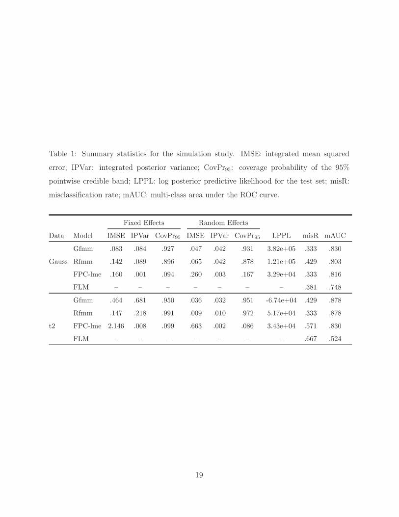
Table 1: Summary statistics for the simulation study. IMSE: integrated mean squared

error; IPVar: integrated posterior variance; CovPr95: coverage probability of the 95%

pointwise credible band; LPPL: log posterior predictive likelihood for the test set; misR:

misclassification rate; mAUC: multi-class area under the ROC curve.

Fixed Effects Random Effects

Data Model IMSE IPVar CovPr95 IMSE IPVar CovPr95 LPPL misR mAUC

Gfmm .083 .084 .927 .047 .042 .931 3.82e+05 .333 .830

Gauss Rfmm .142 .089 .896 .065 .042 .878 1.21e+05 .429 .803

FPC-lme .160 .001 .094 .260 .003 .167 3.29e+04 .333 .816

FLM – – – – – – – .381 .748

Gfmm .464 .681 .950 .036 .032 .951 -6.74e+04 .429 .878

Rfmm .147 .218 .991 .009 .010 .972 5.17e+04 .333 .878

t2 FPC-lme 2.146 .008 .099 .663 .002 .086 3.43e+04 .571 .830

FLM – – – – – – – .667 .524

19

results in very low variability and coverage rate, hence is not effective in characterizing

uncertainty of the estimated parameters. The FLM approach provides a misR higher

than Gfmm but lower than Rfmm, and its mAUC is the lowest among all four models

considered. In the t2 case, we see that the Rfmm results in lower IMSE and IPVar, much

higher LPPL, and lower misR than Gfmm. This suggests that when the data follows

heavier-tailed distributions, Rfmm clearly outperforms Gfmm. Furthermore, Rfmm also

outperforms FPC-lme and FLM with evidently better estimation, higher LPPL, and more

accurate classification.

6 The Sonar-terrain Data Analysis Results

Recall that our goals in analyzing the sonar-terrain data include characterizing the dif-

ferential sonar responses to terrains, identifying differences between channels, and compar-

ing the discrimination performances between the two-channel design and the single-channel

design. Following the automatic workflow described in Section 4.4, we have performed data

analysis based on echo envelopes extracted from the sonar-terrain data. Results are sum-

marized as follows.

Selecting models. First, we performed model selection following the PPO calculation

described in Section 4.1 to determine whether the Gaussian model is sufficient or the robust

model is necessary. The selection was performed using a training-validation procedure. The

whole sonar-terrain data were split into a training set containing 81 footprints (30 from

grass and sand, 21 from rainforest), and a validation set containing 28 footprints (10 from

the grass and sand, 8 from the rainforest). At this stage, each footprint contains 40 echoes,

20 from each channel. We obtained posterior samples of the model parameters from the

training data, and used them to calculate the PPO for the validation data. Results show

that the log(PPO) for Gfmm versus Rfmm is 7.65e+04, providing strong evidence in favor

of the Gaussian model. Therefore, we selected Gfmm for future analysis.

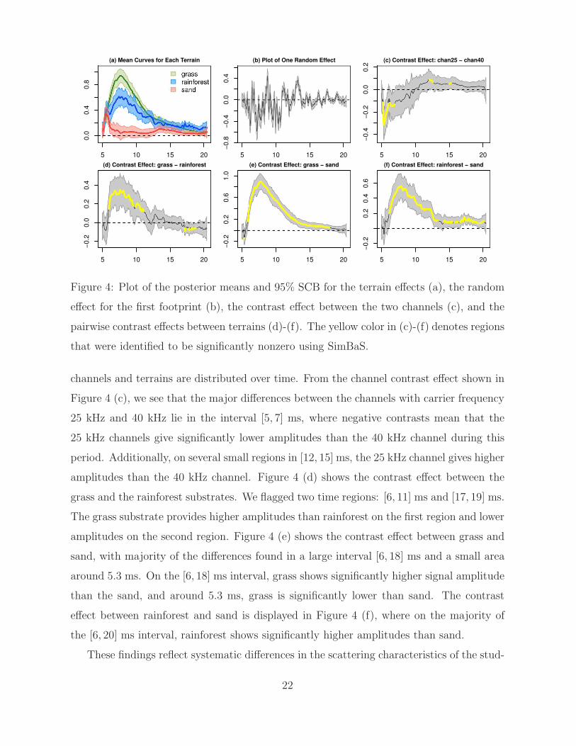
Estimating effects and detecting regions. After selecting the model, we refit

the selected Gfmm to the whole dataset, which contains all 109 footprints from three

terrains and two channels. The fixed effects in G(t) = (G1(t), G2(t), G3(t))T represent the

mean curves for each terrain. Their posterior means and the corresponding 95% SCBs are

20

displayed in Figure 4 (a). We see from Figure 4 (a) that the echo envelopes from the three

terrain substrates demonstrate very different patterns, despite that all showed an increase

at the initial [5, 6] ms and all decay after 15 ms. The grass substrate shows one wide

peak at 8 ms with a monotonic increase before and monotonic decrease after 8 ms. The

rainforest substrate, on the other hand, shows an sharp initial impulse on the interval [5, 6]

ms, followed by a wide peak on the interval [7, 9] ms. The sand substrate only shows a

sharp impulse on the interval [5, 6] ms, followed by low amplitudes on the interval [6, 13] ms

and a slight increase around 13.5 ms. Clear differences in amplitudes are observed on the

time region [7, 13] ms. During this period, the grass substrate gives the highest amplitude,

and the rainforest is lower than the grass but much higher than the sand. The mean curves

represent the signal strength that is common across all terrains but do not characterize

the characteristics of each specific location. The latter is estimated through the footprint

random effects. In Figure 4 (b), we demonstrate the posterior mean and 95% SCB of

the random effect from the first footprint, which shows frequent fluctuations around zero

than the fixed effect estimation. These fluctuations reflect sonar responses to the specific

distribution of the scatterers for that footprint location. All other random effect estimates

demonstrate similar fluctuating behaviors.

To identify “sonar signatures” of different terrains, we flag significantly nonzero regions

on the contrast effects using the SimBaS described in Section 4.2. Since there are three

terrains and two channels, we have three pairwise contrast effects between terrains and one

channel contrast effect. The SimBaS(t) was calculated by simultaneously adjusting across

all four pairs of contrast effects, and GBPVs for the overall tests (H0: all four pairs of the

contrast effects are zero) and for test on each of the contrast effect (H0: C(t) ≡ 0 for one

contrast effect) were calculated. The GBPV results show that both the overall GBPV and

the GBPV for each contrast effect are at the 0.001 level, providing strong evidence that

there are significantly nonzero locations on each contrast effect. We then flagged regions

with SimBaS(t) < α as significantly nonzero. In Figure 4(c)-(f), we plotted the posterior

mean and 95% SCBs for the channel contrast effects and for the pairwise contrast effects

between terrains. The significantly nonzero regions were flagged by the yellow color.

Examining the contrast effects in Figure 4 (c)-(f), we see how the differences between

21

5 10 15 20

0.0

0.4

0.8

(a) Mean Curves for Each Terrain

5 10 15 20

−0.8

−0.4

0.0

0.4

(b) Plot of One Random Effect

5 10 15 20

−0.4

−0.2

0.0

0.2

(c) Contrast Effect: chan25 − chan40

5 10 15 20

−0.2

0.0

0.2

0.4

(d) Contrast Effect: grass − rainforest

5 10 15 20

−0.2

0.2

0.6

1.0

(e) Contrast Effect: grass − sand

5 10 15 20

−0.2

0.2

0.4

0.6

(f) Contrast Effect: rainforest − sand

Figure 4: Plot of the posterior means and 95% SCB for the terrain effects (a), the random

effect for the first footprint (b), the contrast effect between the two channels (c), and the

pairwise contrast effects between terrains (d)-(f). The yellow color in (c)-(f) denotes regions

that were identified to be significantly nonzero using SimBaS.

channels and terrains are distributed over time. From the channel contrast effect shown in

Figure 4 (c), we see that the major differences between the channels with carrier frequency

25 kHz and 40 kHz lie in the interval [5, 7] ms, where negative contrasts mean that the

25 kHz channels give significantly lower amplitudes than the 40 kHz channel during this

period. Additionally, on several small regions in [12, 15] ms, the 25 kHz channel gives higher

amplitudes than the 40 kHz channel. Figure 4 (d) shows the contrast effect between the

grass and the rainforest substrates. We flagged two time regions: [6, 11] ms and [17, 19] ms.

The grass substrate provides higher amplitudes than rainforest on the first region and lower

amplitudes on the second region. Figure 4 (e) shows the contrast effect between grass and

sand, with majority of the differences found in a large interval [6, 18] ms and a small area

around 5.3 ms. On the [6, 18] ms interval, grass shows significantly higher signal amplitude

than the sand, and around 5.3 ms, grass is significantly lower than sand. The contrast

effect between rainforest and sand is displayed in Figure 4 (f), where on the majority of

the [6, 20] ms interval, rainforest shows significantly higher amplitudes than sand.

These findings reflect systematic differences in the scattering characteristics of the stud-

22

ied terrains. For the grass texture, the highest response amplitude occurred around 8 ms,

whereas for sand it occurred earlier (at 5.5 ms) and was more concentrated in time due

to the more compact nature of the terrain surface. The rainforest substrate consists of

scatters of mixed type (e.g, leaves, branches, dirt), hence resulted in both a 5.3 ms peak

and a 8 ms peak. The scattering strength of grass is higher than that of the rainforest, and

they both are much higher than of the sand.

Comparing designs using discriminant analysis. Another question of our inter-

est is whether the two-channel design is more effective than the single-channel designs

in identifying terrains. We answer this question through discriminant analysis based on

echoes collected from two channels versus that from a single channel. To this end, we

re-split the sonar-terrain data into three subsets, Data 1-3, according to Section 4.4. Data

1 represents the two-channel design and Data 2-3 represent the single-channel designs. We

applied Gfmm to each of the three subsets and predicted the terrain types using 4-fold

cross-validation. Classification results are reported based on 90% wavelet compression in

the discriminant analysis.

Since the discrimination is multi-class, we adopt several different approaches to sum-

marize the results. On the top panel of Table 2, we display the classification results of

each dataset using confusion matrices (denoted by ConfM). The classification was based

on the decision rule of designating a class label according to the highest posterior predictive

probability. The confusion matrices demonstrate that several footprints were misclassified

between grass and rainforest, and several footprints from sand were misclassified as rain-

forest. In Table 2, we also list the overall misclassification rates (misR) resulted from the

same decision rule. This statistic shows that the two-channel design gives lower misR than

the two single-channel designs, and the 40 kHz design gives lower misR than the 25 kHz

design.

While using the highest posterior probability as a decision rule is a reasonable choice,

one decision rule can hardly reflect the overall performance of a classifier. To compare the

overall performance without pre-specifying a decision rule, in Figure 5 we plot the empirical

ROC curve for the binary classification problem, classifying each terrain versus the other

two terrains. From these ROC curves, we calculated the area under the ROC curve (AUC)

23

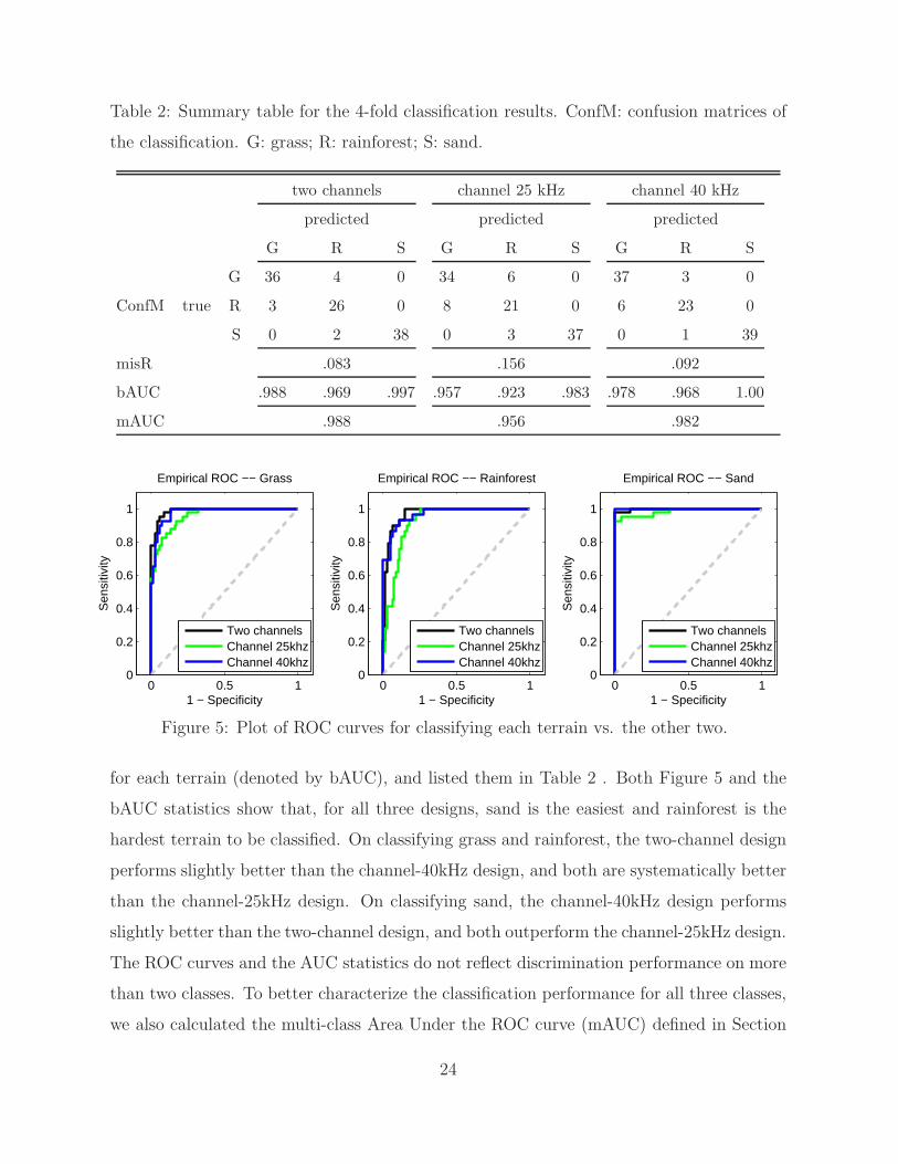
Table 2: Summary table for the 4-fold classification results. ConfM: confusion matrices of

the classification. G: grass; R: rainforest; S: sand.

two channels channel 25 kHz channel 40 kHz

predicted predicted predicted

G R S G R S G R S

G 36 4 0 34 6 0 37 3 0

ConfM true R 3 26 0 8 21 0 6 23 0

S 0 2 38 0 3 37 0 1 39

misR .083 .156 .092

bAUC .988 .969 .997 .957 .923 .983 .978 .968 1.00

mAUC .988 .956 .982

0 0.5 10

0.2

0.4

0.6

0.8

1

1 − Specificity

Sen

sitiv

ity

Empirical ROC −− Grass

Two channelsChannel 25khzChannel 40khz

0 0.5 10

0.2

0.4

0.6

0.8

1

1 − Specificity

Sen

sitiv

ity

Empirical ROC −− Rainforest

Two channelsChannel 25khzChannel 40khz

0 0.5 10

0.2

0.4

0.6

0.8

1

1 − Specificity

Sen

sitiv

ity

Empirical ROC −− Sand

Two channelsChannel 25khzChannel 40khz

Figure 5: Plot of ROC curves for classifying each terrain vs. the other two.

for each terrain (denoted by bAUC), and listed them in Table 2 . Both Figure 5 and the

bAUC statistics show that, for all three designs, sand is the easiest and rainforest is the

hardest terrain to be classified. On classifying grass and rainforest, the two-channel design

performs slightly better than the channel-40kHz design, and both are systematically better

than the channel-25kHz design. On classifying sand, the channel-40kHz design performs

slightly better than the two-channel design, and both outperform the channel-25kHz design.

The ROC curves and the AUC statistics do not reflect discrimination performance on more

than two classes. To better characterize the classification performance for all three classes,

we also calculated the multi-class Area Under the ROC curve (mAUC) defined in Section

24

5. The mAUC results are listed in the bottom row of Table 2, which show that the two-

channel design provides the highest mAUC, whereas the channel-25kHz design gives the

lowest mAUC.

In summary, while different summary statistics provide varied results on the classifica-

tion performance, our discriminant analysis reveals the following systematic facts: (1) Some

terrains are harder to classify than others, e.g., both grass and rainforest result in lower

classification accuracy than sand. (2) Echoes from channels with different carrier frequen-

cies provide different discrimination performance on different terrains. For example, the

two-channel design performs better to classify grass and rainforest, and the channel-40kHz

design performs better in classifying sand. (3) All summary statistics have shown that the

two-channel design achieves target identification performance at least comparable with, or

even better than the signal-channel designs. Given the additional advantage that the dual-

channel design only requires half of the data collection time, we conclude that the multi-

or dual- channel sonar head may be more effective and reliable in target identification than

the single-channel designs.

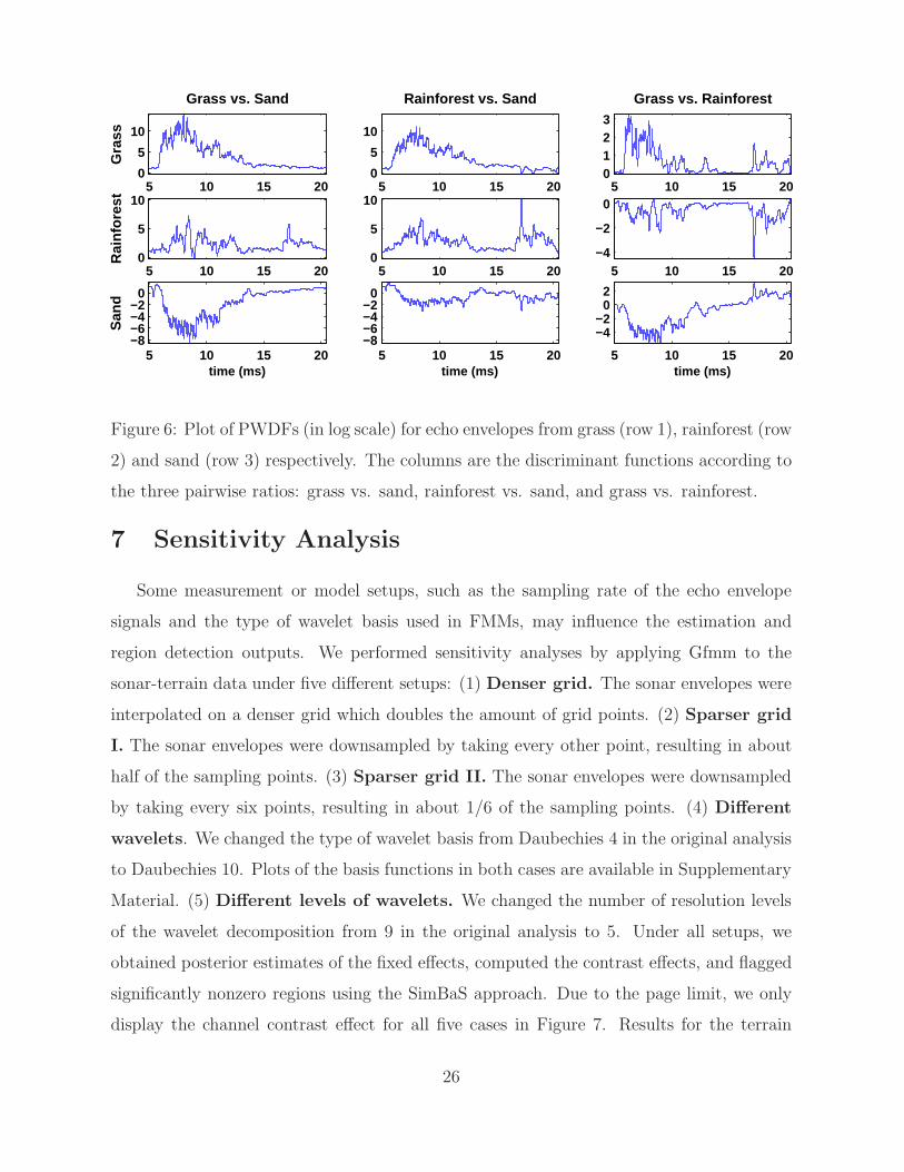
Pointwise Discriminant Functions. To demonstrate local discriminatory perfor-

mance, we calculated the PWDFs (in log scale) and averaged them across all footprints in

each terrain. Results are displayed in Figure 6. The three rows of Figure 6 show the true

terrain type, i.e., whether the results plotted were for echoes collected from grass, rainfor-

est or sand. The three columns of Figure 6 display the discriminant functions according

to the three pairwise ratios. For example, row one and column one shows the mean dis-

criminant function for grass versus sand for echoes collected from grass, where high values

(> 2) indicate strong tendency in favoring grass than sand. From the first row of Figure 6,

we see that for echoes from the grass substrate, the interval [6, 14] ms is the main region

that distinguish grass and rainforest from sand, and the intervals [6, 10] ms and [17, 19] ms

distinguish grass from rainforest. From the second row of Figure 6, we see that for echoes

from the rainforest substrate, the high discriminant regions are [5, 15] ms and [18, 20] ms.

The third row of Figure 6 show that for echoes from the sand substrate, the interval [6, 13]

ms distinguishes sand from grass, and the intervals [7, 13] ms and [17, 19] ms distinguish

sand from rainforest.

25

5 10 15 200

5

10

Grass vs. SandG

rass

5 10 15 200

5

10

Rainforest vs. Sand

5 10 15 200123

Grass vs. Rainforest

5 10 15 200

5

10

Rai

nfor

est

5 10 15 200

5

10

5 10 15 20−4

−2

0

5 10 15 20−8−6−4−2

0

time (ms)

San

d

5 10 15 20−8−6−4−2

0

time (ms)5 10 15 20

−4−2

02

time (ms)

Figure 6: Plot of PWDFs (in log scale) for echo envelopes from grass (row 1), rainforest (row

2) and sand (row 3) respectively. The columns are the discriminant functions according to

the three pairwise ratios: grass vs. sand, rainforest vs. sand, and grass vs. rainforest.

7 Sensitivity Analysis

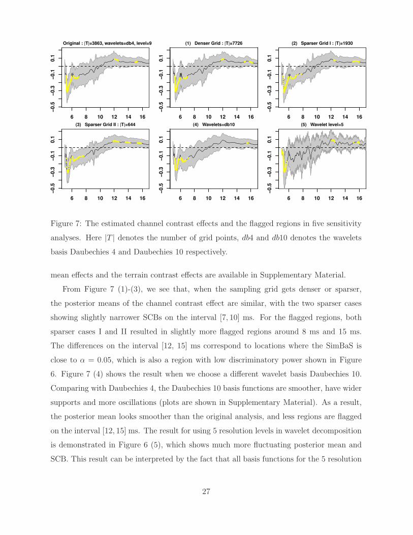
Some measurement or model setups, such as the sampling rate of the echo envelope

signals and the type of wavelet basis used in FMMs, may influence the estimation and

region detection outputs. We performed sensitivity analyses by applying Gfmm to the

sonar-terrain data under five different setups: (1) Denser grid. The sonar envelopes were

interpolated on a denser grid which doubles the amount of grid points. (2) Sparser grid

I. The sonar envelopes were downsampled by taking every other point, resulting in about

half of the sampling points. (3) Sparser grid II. The sonar envelopes were downsampled

by taking every six points, resulting in about 1/6 of the sampling points. (4) Different

wavelets. We changed the type of wavelet basis from Daubechies 4 in the original analysis

to Daubechies 10. Plots of the basis functions in both cases are available in Supplementary

Material. (5) Different levels of wavelets. We changed the number of resolution levels

of the wavelet decomposition from 9 in the original analysis to 5. Under all setups, we

obtained posterior estimates of the fixed effects, computed the contrast effects, and flagged

significantly nonzero regions using the SimBaS approach. Due to the page limit, we only

display the channel contrast effect for all five cases in Figure 7. Results for the terrain

26

6 8 10 12 14 16

−0

.5−

0.3

−0

.10

.1

Original : |T|=3863, wavelets=db4, level=9

6 8 10 12 14 16

−0

.5−

0.3

−0

.10

.1

(1) Denser Grid : |T|=7726

6 8 10 12 14 16

−0

.5−

0.3

−0

.10

.1

(2) Sparser Grid I : |T|=1930

6 8 10 12 14 16

−0

.5−

0.3

−0

.10

.1

(3) Sparser Grid II : |T|=644

6 8 10 12 14 16

−0

.5−

0.3

−0

.10

.1

(4) Wavelets=db10

6 8 10 12 14 16

−0

.5−

0.3

−0

.10

.1

(5) Wavelet level=5

Figure 7: The estimated channel contrast effects and the flagged regions in five sensitivity

analyses. Here |T | denotes the number of grid points, db4 and db10 denotes the wavelets

basis Daubechies 4 and Daubechies 10 respectively.

mean effects and the terrain contrast effects are available in Supplementary Material.

From Figure 7 (1)-(3), we see that, when the sampling grid gets denser or sparser,

the posterior means of the channel contrast effect are similar, with the two sparser cases

showing slightly narrower SCBs on the interval [7, 10] ms. For the flagged regions, both

sparser cases I and II resulted in slightly more flagged regions around 8 ms and 15 ms.

The differences on the interval [12, 15] ms correspond to locations where the SimBaS is

close to α = 0.05, which is also a region with low discriminatory power shown in Figure

6. Figure 7 (4) shows the result when we choose a different wavelet basis Daubechies 10.

Comparing with Daubechies 4, the Daubechies 10 basis functions are smoother, have wider

supports and more oscillations (plots are shown in Supplementary Material). As a result,

the posterior mean looks smoother than the original analysis, and less regions are flagged

on the interval [12, 15] ms. The result for using 5 resolution levels in wavelet decomposition

is demonstrated in Figure 6 (5), which shows much more fluctuating posterior mean and

SCB. This result can be interpreted by the fact that all basis functions for the 5 resolution

27

level setup have very narrow supports (plots are shown in Supplementary Material), thus a

setup with too few resolution levels is less effective in borrowing information across nearby

points.

In summary, we conclude that using denser or moderately sparser grid (e.g., Sparser grid

I) leads to similar posterior estimates and flagged regions. Differences in flagged regions are

mostly observed in places with low discriminatory power. Wavelet basis and the number

of resolution levels should be set so that the basis functions have appropriate supports,

especially at lower resolution levels.

8 Conclusion and Discussion

We have proposed a unified analytical framework to characterize the sonar responses

to different terrain substrates and investigate the performance of a dual-channel sonar de-

sign. The proposed framework relies on functional response regression models—Gfmm and

Rfmm—that flexibly capture the complex data structure while allowing potential outliers

and outlying regions in data. Our Bayesian modeling approach yields intuitive and natural

inferential summaries that adjust for FWER in the inherent multiple testing problem. It

also naturally facilitates model selection and terrain discrimination.

Our application to the sonar-terrain data identifies dynamic regions that reflect signif-

icant differences across pairs of terrains and across the two channels. The discriminant

analysis implies that channels with different carrier frequencies vary in their discrimina-

tory performance under different terrain substrates, and suggests that using channels with

varying carrier frequencies may result in more efficient and reliable target identification.

The most prominent feature of our modeling strategy is its ability to allow various

inferences under the same FMM framework, including selecting among different models,

estimating the effects of terrains on echo responses, identifying local regions with significant

effects, discriminating the terrain types, and identifying local regions with high discrimina-

tory power. These inferences were achieved through an automated workflow that involves

multiple stages and modules for different tasks. This framework provides a model for

automated and rigorous analysis of structured functional data with similar complexity.

One might wonder why we treat the envelopes as responses and not predictors. Modeling

28

using functional response regression is a key strategy for our analysis. It enables us to

account for the inter-function correlations and yet still classify terrains using functional

linear discriminant analysis, while functional predictor regression approaches to date, e.g.,

Cardot et al. (1999) and Muller and Stadtmuller (2005), cannot capture the inter-function

correlation inherent to these data (Morris, 2015).

In this paper, we focused on wavelet representations of the echo envelope data by tak-

ing advantage of its nice properties, including whitening, multi-resolution representation,

allowing for denoising and compression, as well as its ability in capturing nonstationary

and local effects. Depending on characteristics of the data, other basis such as splines and

eigen-functions can also be used for dual space modeling as discussed in Morris et al. (2011)

and Meyer et al. (2015).

SUPPLEMENTARY MATERIALS

Supplementary text: The sonar-terrain experimental setup; the MCMC algorithms for

Gfmm and Rfmm; the computational details for model selection and discrimination;

and additional results on the sensitivity analysis. (pdf)

ACKNOWLEDGEMENTS

The authors thank the Editor-Elect, the Associate Editor and two referees for their

insightful comments. Hongxiao Zhu was supported by Institute for Critical Technology

and Applied Science, Virginia Tech (ICTAS-JFC 175139) and National Science Foundation

(NSF-DMS 1611901). Jeffrey S. Morris was supported by National Cancer Institute (R01-

CA107304, R01-CA178744, P30-CA016672) and National Institute of Drug Abuse (R01-

DA017073). Rolf Muller was supported by National Science Foundation (NSF 1362886)

and Naval Engineering Education Consortium (NEEC, N00174-16-C-0026).

References

Bozma, O. (1994), “A physical model-based analysis of heterogeneous environments using

sonar-ENDURA method,” Pattern Anal. and Mach. Intell., 16(5), 497–506.

29

Cardot, H., Ferraty, F., and Sarda, P. (1999), “Functional linear model,” Stat. Probabil.

Lett., 45, 11–22.

Crainiceanu, C. M., Staicu, A.-M., Ray, S., and Punjabi, N. (2012), “Bootstrap-based

inference on the difference in the means of two correlated functional processes,” Stat.

Med., 31(26), 3223–3240.

Davidson, D. (2009), “Functional mixed-effect models for Electrophysiological responses,”

Neurophysiology, 41(1), 71–79.

Fahner, M., Thomas, J., Ramirez, K., and Boehm, J. (2004), “Acoustic properties of

echolocation signals by captive Pacific white-sided dolphins,” in Echolocation in bats and

dolphins, eds. J. A. Thomas, C. F. Moss, and M. Vater, Chicago: University of Chicago

Press, chapter 9, pp. 53–59.

Guo, W. (2002), “Functional mixed effects models,” Biometrics, 58, 121–128.

Hand, D. J., and Till, R. J. (2001), “A simple generalisation of the area under the ROC

curve for multiple class classification problems,” Mach. Learn., 45, 171 – 186.

Kleeman, L., and Kuc, R. (1995), “Mobile robot sonar for target localization and classifi-

cation,” Int. J. of Robot. Res., 14(4), 295–318.

Kong, D., Xue, K., Yao, F., and Zhang, H. H. (2016), “Partially functional linear regression

in high dimensions,” Biometrika, 103(1), 147–159.

Kuc, R. (2001), “Pseudo-amplitude scan sonar maps,” IEEE Trans. Robot. Autom.,

17(5), 767–770.

Lancia, L., Rausch, P., and Morris, J. S. (2015), “Automated quantitative analysis of

ultrasound tongue contours via wavelet-based functional mixed models,” J. Acoust. Soc.

Am., 137, EL178–EL183.

Le Chevalier, F. (2002), Principles of Radar and Sonar Signal Processing, Norwood, MA

USA: Artech House, Inc.

30

Lee, W., and Morris, J. S. (2016), “Identification of differentially methylated loci using

wavelet-based functional mixed models,” Bioinformatics, 32(5), 664–672.

Martinez, J. G., Bohn, K. M., Carroll, R. J., and Morris, J. S. (2013), “A study of Mexi-

can free-tailed bat chirp syllables: Bayesian functional mixed models for nonstationary

acoustic time series,” J. Am. Stat. Assoc., 108(502), 514 – 526.

Meyer, M. J., Coull, B. A., Versace, F., Cinciripini, P., and Morris, J. S. (2015), “Bayesian

function-on-function regression for multilevel functional data,” Biometrics, .

Morris, J. S. (2015), “Functional Regression,” Annu Rev Stat Appl., 2, 321–359.

Morris, J. S., Baladandayuthapani, V., Herrick, R. C., Sanna, P., and Gutstein, H. (2011),

“Automated analysis of quantitative image data using isomorphic functional mixed mod-

els, with application to proteomics data,” Ann. Appl. Stat., 5, 894–923.

Morris, J. S., Brown, P. J., Herrick, R. C., Baggerly, K. A., and Coombes, K. R. (2008),

“Bayesian analysis of mass spectrometry proteomic data using wavelet-based functional

mixed models,” Biometrics, 64, 479–489.

Morris, J. S., and Carroll, R. J. (2006), “Wavelet-Based functional mixed models,” J. R.

Stat. Soc. Ser. B, 68, 179–199.

Muller, H., and Stadtmuller, U. (2005), “Generalized Functional Linear Models,” The

Annals of Statistics, 33(2), 774–805.

Muller, R. (2003), “A computational theory for the classification of natural biosonar targets

based on a spike code,” Comput. Neural. Syst., 14, 595–612.

Muller, R., and Kuc, R. (2000), “Foliage echoes: A probe into the ecological acoustics of

bat echolocation,” J. Acoust. Soc. Am., 108, 836–845.

Phillip, M., and Kristiansen, B. (2006), “Classifying surface roughness with CTFM ultra-

sonic sensing,” IEEE Sensors Journal, 6(5), 1267–1279.

Ramsay, J. O., and Silverman, B. W. (1997), Functional Data Analysis, New York:

Springer-Verlag.

31

Reyes Reyes, M. V., In ıguez, M. A., Hevia, M., Hildebrand, J. A., and Melcon, M. L.

(2015), “Description and clustering of echolocation signals of Commerson’s dolphins

(Cephalorhynchus commersonii) in Bahıa San Julian, Argentina,” J. Acoust. Soc. Am.,

138(4), 2046–2053.

Robertson, C. J. (1996), “Statistical analysis of sonar data for target detection,”.

URL: http://dx.doi.org/10.1117/12.241216

Ruppert, D., Wand, M. P., and Carroll, R. J. (2003), Semiparametric Regression, Cam-

bridge Series in Statistical and Probabilistic Mathematics, UK: Cambridge University

Press.

Vicente Martinez Diaz, J. (n.d.), “Analysis of multibeam sonar data for the characterization

of seafloor habitats,”.

Von Helversen, D. (2004), “Object classification by echolocation in nectar feeding bats:

size-independent generalization of shape,” J. Comp. Physiol. A., 190, 515–521.

Witkovsky, V. (2001), “MATLAB algorithm mixed.m for solving Hendersons mixed model

equations,”, Technical report, Institute of Measurement Science, Slovak Academy of

Sciences.

Yao, F. (2007), “Asymptotic distributions of nonparametric regression estimators for lon-

gitudinal or functional data,” J. of Multivariate Anal., 98, 40–56.

Yovel, Y., Franz, M. O., Stilz, P., and Schnitzler, H. U. (2008), “Plant classification from

bat-like echolocation signals,” PLoS Comput. Biol., 4(3).

Yovel, Y., Stilz, P., Franz, M. O., Boonman, A., and Schnitzler, H.-U. (2009), “What a

plant sounds like: the statistics of vegetation echoes as received by echolocating bats,”

PLoS Comput. Biol., 5(7).

Zhu, H., Brown, P. J., and Morris, J. S. (2011), “Robust, adaptive functional regression in

functional mixed model framework,” J. Am. Statist. Ass., 495, 1167–1179.

Zhu, H., Brown, P. J., and Morris, J. S. (2012), “Robust classification of functional and

quantitative image data using functional mixed models,” Biometrics, 68(4), 1260–1268.

32