Embed Size (px)
Citation preview
A Two-Way Semi-Linear Model for Normalization and Analysisof cDNA Microarray Data
Jian Huang, Deli Wang and Cun-Hui Zhang
ABSTRACT A basic question in analyzing cDNA microarray data is normalization, the purpose
of which is to remove systematic bias in the observed expression values by establishing anormalization curve across the whole dynamic range. A proper normalization procedure ensures
that the normalized intensity ratios provide meaningful measures of relative expression levels. Wepropose a two-way semi-linear model (TW-SLM) for normalization and analysis of microarraydata. This method does not make the usual assumptions underlying some of the existing methods.
For example, it does not assume that: (i) the percentage of differentially expressed genes is small;or (ii) there is symmetry in the expression levels of up- and down-regulated genes, as required
in the lowess normalization method. The TW-SLM also naturally incorporates uncertainty due tonormalization into significance analysis of microarrays. We use a semiparametric approach based
on polynomial splines in the TW-SLM to estimate the normalization curves and the normalizedexpression values. We study the theoretical properties of the proposed estimator in the TW-SLM,including the finite sample distributional properties of the estimated gene effects and the rate of
convergence of the estimated normalization curves when the number of genes under study is large.We also conduct simulation studies to evaluate the TW-SLM method and illustrate the proposed
method using a published microarray data set.
KEY WORDS: differentially expressed genes; microarray; high-dimensional data; semiparametricregression; spline; analysis of variance; noise level; variance estimation.
Jian Huang is Professor, Department of Statistics and Actuarial Science and Program in Public
Health Genetics, University of Iowa, Iowa City, IA 52242 (Email: [email protected]). DeliWang is Research Assistant Professor, Biostatistics and Bioinformatics Unit, Comprehensive
Cancer Center, University of Alabama at Birmingham, Birmingham, AL 35294 (Email:[email protected]). Cun-Hui Zhang is Professor, Department of Statistics, Rutgers
University, Piscataway, NJ 08855 (Email: [email protected]). The research of Huang issupported in part by the NIH grants MH001541 and HL72288-01 and an Iowa Informatics Initiativegrant. The research of Zhang is partially supported by the NSF grants DMS-0102529 and DMS-
0203086. The authors thank the Editor, the Associate Editor and two anonymous reviewers fortheir helpful comments that led to substantial improvement in the paper. The authors also thank
Professor Terry Speed and his collaborators for making the Apo A1 data set available online. Thisdata set is used as an example in this paper.
1
1. Introduction Microarray technology has become a useful tool for quantitatively monitoringgene expression patterns and has been widely used in functional genomics (Schena, Shalon, Davis
and Brown 1995; Brown and Botstein 1999). In a cDNA microarray experiment, cDNA segmentsrepresenting the collection of genes and expression sequence tags (ESTs) to be probed are amplifiedby PCR and spotted in high density on glass microscope slides using a robotic system. Such slides
are called microarrays. Each microarray contains thousands of reporters of the collection of genesor ESTs. The microarrays are queried in a co-hybridization assay using two fluorescently labeled
biosamples prepared from the cell populations of interest. One sample is labeled with fluorescentdye Cy5 (red), and another with fluorescent dye Cy3 (green). Hybridization is assayed using a
confocal laser scanner to measure fluorescence intensities, allowing simultaneous determination ofthe relative expression levels of all the genes represented on the slide (Hedge, Qi, Abernathy, Gay,Dharap, Gaspard, Earle-Hughes, Snesrud, Lee and Quackenbush 2000).
A basic question in analyzing cDNA microarray data is normalization, the purpose of which isto remove systematic bias in the observed expression values by establishing a normalization curve
across the whole dynamic range. A proper normalization procedure ensures that the normalizedintensity ratios provide meaningful measures of relative expression levels. Normalization is needed
because many factors, including differential efficiency of dye incorporation, difference in theamount of RNA labeled between the two channels, uneven hybridizations, differences in the
printing pin heads, among others, may cause bias in the observed expression values. Therefore,proper normalization is a critical component in the analysis of microarray data and can haveimportant impact on higher level analysis such as detection of differentially expression genes,
classification, and cluster analysis.Yang, Dudoit, Luu and Speed (2001) systematically considered several normalization methods,
including global, intensity-dependent, and dye-swap normalization. The global normalizationmethod assumes a constant normalization factor for all the genes and re-scales the red and green
channel intensities so that the mean or median of the intensity log-ratios is zero. For intensity-dependent normalization, Yang et al. (2001) proposed using the locally weighted linear scatterplotsmoother (lowess, Cleveland 1979) in the scatter plot of log-intensity ratio versus log-intensity
product (the M-A plot) and uses the resulting residuals as the normalized log-intensity ratios. Theanalysis of variance (ANOVA) method (Kerr, Martin and Churchill 2000) and the mixed linear
model method (Wolfinger, Gibson, Wolfinger, Bennett, Hamadeh, Bushel, Afshari and Paules 2001)takes into account array and dye effects among others in a linear model framework, and assumes
constant normalization factors. Fan, Tam, Woude and Ren (2004) proposed a Semi-Linear In-slideModel (SLIM) method that makes use of replications of a subset of the genes in an array. Fan,
Peng and Huang (2004) generalized the SLIM method to account for across-array information,resulting in an aggregated SLIM, so that replication within an array is no longer required. Park, Yi,Kang, Lee, Lee and Simon (2003) conducted comparisons of a number of normalization methods,
including global, linear and lowess normalization methods. All the methods described above,
2
except the ANOVA method, treat normalization as a step separated from the subsequent significantanalysis, in which the variation due to normalization is not taken into account.
The lowess normalization is one of the most widely used normalization methods. It assumesthat at least one of the two biological assumptions is satisfied: (i) the proportion of differentiallyexpressed genes should be small, or (ii) there is symmetry in the expression values between up
and down regulated genes. These two assumptions reduce the possibility that the differentiallyexpressed genes are incorrectly “normalized.” For experiments where these two assumptions are
violated, the lowess normalization method is not appropriate. Yang et al. (2001) suggested usingdye-swap normalization. This approach makes the assumption that the normalization curves in
the two dye-swaped slides are the same. Because of slide-to-slide variation, this assumption maynot always be satisfied. To alleviate the dependence of the lowess normalization method on theassumption (i) or (ii) stated above, Tseng, Oh, Rohlin, Liao and Wong (2001) proposed using a rank
based procedure to first select a set of invariant genes that are likely to be constantly expressed,and then carrying out lowess normalization using this set of genes. However, they pointed out
that the set of selected genes may be relatively small and not cover the whole dynamic range ofthe expression values, and extrapolation is needed to fill in the gaps that are not covered by the
invariant genes.We propose a two-way semi-linear model (TW-SLM) for normalization of cDNA microarray
data. This model is motivated in part by examining the lowess normalization from thesemiparametric regression point of view. The TW-SLM normalization method does not makethe assumptions underlying the lowess normalization method, nor does it require pre-selection
of invariant genes or replicated genes in an array. The TW-SLM also provides a framework forincorporating variability due to normalization into significance analysis of microarray data. Below,
we first describe the TW-SLM for microarray data. In Section 3, we describe a Gauss-Seidelalgorithm for computing the normalization curves and the estimated relative expression values
based on the TW-SLM model. In Section 4, we present a method for detecting differentiallyexpressed genes based on the TW-SLM. In Section 5, we provide theoretical results for theproposed estimators of TW-SLM. In Section 6, we illustrate the proposed method by an example.
We also use simulation to compare the proposed method with the lowess normalization methodand an analogue of the lowess method where splines are used in the curve fitting instead of local
regression. Some concluding remarks are given in Section 7.
2. A two-way semi-linear model for microarray data To motivate the proposed TW-SLMmodel for normalization, we first give a description of the lowess normalization method from the
semiparametric regression point of view. Because the proposed TW-SLM can be considered as anextension of the standard semiparametric regression model (SRM) (Wahba 1984; Engel, Granger,
Rice and Weiss 1986), we also give a brief description of this model.
2.1. The lowess normalization Suppose that there are�
genes and � arrays in the study and thateach gene is spotted once in an array. Let ����� and ����� be the intensity levels of gene in array
3

from the type 1 and type 2 samples, respectively. Following Chen, Daugherty and Bittner (1997)and Yang et al. (2001), let � ��� be the log-intensity ratio of the th gene in the th array, and let �����be the corresponding average of the log-intensity. That is,
������������ � ���� ����� � ��� ��� ������ � ��� ��� ��� � ��
���������� � � ��
����������
�� (1)
For the th array �� ���������� � , the lowess normalization fits the nonparametric regression
��������� ����� �������! #"��� � ������������
�� (2)
using Cleveland’s lowess method. Let $� � be the lowess estimator of ��� , and let the residuals from
the nonparametric curve fitting be
$ "��� �%� ���'& $� ����� ����� � ������������ � � (�
����������
��
These residuals are defined as the normalized data and used as the input in the subsequent analysis.So usually the overall analysis consists of two steps: (i) normalization; and (ii) analysis based
on normalized data $ "��� . For example, in comparing two DNA samples using a direct comparisondesign (i.e., the two cDNA samples are competitively hybridized on an array), a typical approach
is to first normalize the data using the lowess normalization, and then to make inference aboutdifferentially expressed genes based on the normalized data. The underlying statistical framework
of such a two-step analysis in the direct comparison design can be described using two models. Thefirst is the nonparametric regression for normalization given in (2). The second model concerns theresidual:
#"��� �*) �+�! ��� � (3)
where ) � is the underlying relative expression value of gene . The goal of the significance analysisis to detect genes with ) �-,�*. . In the two-step approach, (2) and (3) are used as stand-alone models
for each of the two steps, and the effects of the approximation $ "���-/ "� � are typically completelyignored in the analysis.
The lowess normalization is usually applied using all the genes in a study. In general, if allthe genes are used, the differentially expressed genes may be incorrectly “normalized,” since such
genes tend to pull the normalization curve towards themselves. Thus the two-step analysis approachmay yield biased estimators of both ��� and ) � and inefficient test statistics for the inference of ) �(e.g. relatively large p-values for two-sided tests compared with more efficient procedures).
2.2. The semiparametric regression model Suppose that the data consist of � triplets�0��� � � � �21 �3� � ��
���������� � , where � � is the response variable, and �3� � �21 �0� is the covariate. The SRM is
� �4���5�3� �3��� 16� )7�8 � � ��
��������9� � � (4)
where � is an unknown function, ) is the regression parameter, and � is the residual. Thismodel is useful in many situations, for example, when 1 � is a dichotomous variable representing
4
two conditions (treatment versus placebo etc.) and we are interested in the treatment effect )but need to adjust for the effect of the continuous covariate ��� . For a � -dimensional covariate� ��� �3� ��� ��������� � ��� �
6, it is useful to impose an additive structure on � (Hastie and Tibshirani 1990).
A semiparametric generalized additive model is
� �4�������3��� ��� ����� �� �3��� �3��� 16� )7�8 � � ��
���������� � � (5)
Models (4) and (5) are two basic semiparametric models. There are two important
considerations about parameter estimation in (4) and (5). First, both � and ) should be estimatedjointly. For example, it is incorrect to fix ) at 0, obtain an estimate of � , then treat this estimateof � as a known quantity, substitute it back into (4), and then estimate ) . Second, the uncertainty
due to estimation of � generally needs to be taken into account in estimating ) , according to thesemiparametric information theory, see for instance, Bickel, Klaassen, Ritov and Wellner (1993),
pages 107-109.
2.3. The two-way semi-linear model We first describe the proposed model for the special case ofa direct comparison design, in which two cDNA samples from the respective cell populations are
competitively hybridized on the same array. Let � � � and � ��� be the log-intensity ratio and productdefined in (1). The proposed (simple) TW-SLM is
� � ����� ���3� � �����!) �+�! ��� � �� ���������� � � (�
����������
�� (6)
where � � is the intensity-dependent normalization curve for the th array, ) � ��� represents the
normalized relative expression values of gene , and ��� has mean 0 and variance � � � .The TW-SLM can be considered as a combination of the two models that are implicitly used
in the lowess normalization (2) and (3). Specifically, we obtain (6) by simply substituting (3) into(2). Combining these two models enables us to estimate normalization curves and gene effects
simultaneously. This is desirable, since we typically do not know which genes are constantlyexpressed (i.e., with ) � � . ). Approximately unbiased normalization could be carried out usingonly constantly expressed genes if a large set of such genes can be identified, but this is rarely the
reality.We call (6) a two-way model because it also can be considered as a semiparametric
generalization of the two-way ANOVA model. That is, when � �(��� � � ���������9� � , where � �
is a constant parameter, (6) simplifies to the two-way ANOVA. The TW-SLM is an extension of but
different from the SRM (4). Clearly it is also different from the semiparametric generalized additivemodel (5). In particular, in models (4) and (5), the number of finite- and infinite-dimensional
parameters is fixed and is independent of the sample size, and they do not include the standardtwo-way ANOVA as a submodel. In contrast, in the TW-SLM, the number of finite-dimensionalparameters is
�, which is the sample size for estimating � � , and the number of infinite-dimensional
parameters is � , which is the sample size for estimating ) � .
5
In general, let 1 � � ��
be a covariate vector associated with the th array. The proposed(general) TW-SLM is:
� � ��� � � �3� ������� 16� ) � �! ��� � �
��������9� � � ��
����������
�� (7)
where ) � � � � is the effect associated with the th gene, and where � � and ��� are the same as in(6).
The covariate vector 1 � can be used to code various design schemes, such as the loop, reference,and factorial designs (Kerr and Churchill 2001). For example, for the two-sample direct comparison
design, 1 � ��� �
���������� � , which is model (6). For an indirect comparison design using a
common reference, we can introduce a two-dimensional covariate vector 1 ��� � 1 ��� � 1 � �6. Let 1 ���� � � . �
6if the th array is of the type 1 sample versus the reference, and 1 � � � . �
� � 6 if the th arrayis of the type 2 sample versus the reference. Now ) � � �0) � � � ) � �
6is a two-dimensional vector
and ) ��5&!) � represents the difference in the expression levels of gene after normalization. The
covariate 1 � can also include other factors such as covariates and block effects that contribute to thevariations of the observed expression values.
In model (7), it is only made explicit that the normalization curve � � is array-dependent. It isstraightforward to extend the model so that � � also depends on the printing-pin blocks within an
array. This can be achieved by simply treating each block as an array and apply the TW-SLM atthe block level. We can also adapt the TW-SLM to other designs such as multiple spotting and
incorporate spiked control genes in the TW-SLM. Multiple spotting is helpful for improving theprecision and for assessing the quality of an array using the coefficient of variation (Tseng et al.2001). Spike genes can be used for the purpose of calibration and for helping with normalization
in an experiment.
3. TW-SLM normalization We now define the semiparametric least squares estimator (SLSE) inthe TW-SLM and describe an algorithm for computing the estimated normalization curves and geneexpression values using the TW-SLM. Many nonparametric smoothing procedures can be used for
this purpose. We use the method of polynomial splines (Schumaker 1981). This method is easy toimplement, and has similar performance as other nonparametric curve estimation methods such as
local polynomial regression and smoothing splines (Hastie, Tibshirani and Friedman 2001).
3.1. Semiparametric LS estimator in TW-SLM Let����� �� be the space of all
���matrices � �
�0) � ��������� ) � � 6 satisfying ���� � ) ����. . It is clear from the definition of the TW-SLM model (7) that� is identifiable only up to a member in
����� �� , since we may simply replace ) � by ) � & �� � � ) ��� �and � ���3� � by � � �3� ��� �� � � ) 6� 1 � � � in (7). In what follows, we assume
� �� ��� �� ��� ��� ��
��� � ) � �*.�� � (8)
Let � ��� �������9� � ��� �! be " � B-spline base functions. Let# � � $%� � � �3� � � �� � � � �3� � �'& � �
��������� " �)( (9)
6
be the spaces of all linear combinations of the basis functions. We approximate � � by� � � � �! � � � � � � �3� � � � � � � ����� � 6 � � �
# � � where � ����� �*� � � � � ������� � ��������� � ��� �! ��� � � 6 , and � � �� � � � � � ��� �������9� � � �! 0� 6 are coefficients to be estimated from the data. Let � � � � � ��������� ��� � and� � �0) � ��������� ) � � 6 . The LS objective function is� � � � �+�+� ��
� � ���
��� �� � ���'&8� � ��� �����5& 1
6� ) ��� �
We define the semiparametric least squares estimator (SLSE) of $ � � � ( to be the $ $� � $� ( �� ��� �� �� �� � � # � that minimizes
� � � � �+� . That is,
��$� � $�+� � �� �� ������� � ��������� �"!# �%$'& )(%*�+ � � � � � � � (10)
Let , ��� � � � � � ������� ����� ��������� � ��� �! ��� ����� � 6 be the spline basis functions evaluated at ��� � ��.- -
� ��/- - �
. The spline basis matrix for the th array is , ��� �0, 6��� ��������� , 6� � � where , ��� �� � � � �����3� � ��� ��������� � � �! �3� ����� � 6 . Let 1 � � � � ��������� �2�� 6 . We can write
� � � � 1 ��� � � � � �+� . Then
the problem of minimizing� � � � 1 � with respect to � � � 1 � is equivalent to solving the linear
equations:
$� ��� � � � 1 � 1
6� ���
��� � � , � $� � 1
6� �
��� � � 3 � 1 6� � , ��, 6� $� � �4, 6� $� 1 �4�5, 6� 3 � �
Let � $� � $1 � be the solution. We define 6� ����� � �7� � �3� � 6 $� � � �� ���������� � .
3.2. Computation Our approach for minimizing� � � � 1 � is to use the Gauss-Seidel method, also
called the back-fitting algorithm (Hastie, Tibshirani and Friedman 2001), that alternately updates1 and � . Set � � � � �98 . For & ��. ����������� ,
Step 1: Compute 1 � � � by minimizing� � � � � �
� 1 � with respect to 1 . The explicit solution is
�� � �� � �0, 6� , �0�;: � , 6� � 3 � & � � � �
1 �0� � ������������ � �
Step 2: Given the 1 � � � computed in Step 1, let �� � �� �3� �!� � ����� � 6 � � � �� , compute � � �;< �=�
by
minimizing�?> � � � 1 � � � � with respect to � . The explicit solution is
$)� �;< �=�� �
@ ��� � � 1 � 1
6�BA : � ��
� � � 1 � C������ & �� � �� ��� �����ED � �� �
����������� (11)
Iterate between Steps 1 and 2 until the desired convergence criterion is satisfied. Because
the objective function is strictly convex, the algorithm converges to the sum of residual squares.Suppose that the algorithm meets the convergence criterion at step " . Then the estimated valuesof ) � are $) ����)
� �'�� � -�����������
�, and the estimated normalization curves are
$� � �3� � �F� ���3� � 6 � � �'�� �7� ���3� � 6 �=, 6� , �3� : � , 6� � 3 � & $� 1 �3� � �� ��������9� � � (12)
7

The algorithm described above can be conveniently implemented in the statistical computingenvironment R (R Development Core Team 2003). Specifically, Steps 1 and 2 can be solved by the
function lm in R. The function bs can be used to create a basis matrix for the polynomial splines.Let � � � �3� � � ��������� � � � � 6 and � ����� �0� � � � ���3� � � � ��������� � ���3� � � � � 6 . Let
� � � , � �=, 6� , �3� : � , 6� . By(12), the estimator of ��� ��� �3� is
$� ����� �3� � � � � 3 � & $� 1 �0� �Thus the normalization curve is the result of the linear smoother
� � operating on 3 � & $� 1 � . The geneeffect $� 1 � is removed from 3 � . In comparison, the lowess normalization method does not remove
the gene effect. An analogue of the lowess normalization, but using polynomial splines, is�� ����� �3�+� � � 3 � � , � 1 � � �
� � (13)
Comparing $� � ��� �3� with�� ����� �3� , if there is a relatively large percentage of differentially expressed
genes, the difference between this two normalization curves can be large. The magnitude of thedifference also depends on the magnitude of the gene effects.
4. TW-SLM for significant analysis of microarray data In addition to being a stand-alone modelfor normalization, the TW-SLM can also be naturally used for detection of differentially expressed
genes. For the purpose of making inference about � , we need to estimate the variance of $� . Below,we first consider the structure of $� , and then describe an intensity dependent variance estimator.
4.1. Structure of the semiparametric LS estimator We give the expression of $� and define the
observed information matrix for � in the presence of the normalization curves � � � ����������� � .
Let � � � �3� ��� ��������� � � � � 6 � 3 � � �3� ��� ��������� � � � � 6 and � ��� �0� � � � �3� ��� � ��������� � ��� � � � � 6 for a univariate
function � . We write the TW-SLM (7) in vector notation as3 � � � 1 � � � � ��� �3����� � � �� ���������� � � (14)
Using (14), it can be shown that the SLSE (10) equals
$� �5�� � ����� ��� � �
���� 3 � &*��� � & � �0� � 1 ����� � (15)
In the special case of model (6), � �
(scalar ) � ) and � is a vector in R � , (15) is explicitly
$� � $ : �� � � � �� ��� � � ��� � & � �0� 3 � 1 6�� � (16)
since � � & � � are projections in R � , where 1 �4��
(scalar) and, where
$ � � � � ��
��� � � ��� � & � ��� � (17)
8
We note that $ � � � can be considered as the observed information matrix. Here and below, � : �denotes the generalized inverse of matrix � , defined by � : � � � �� � �������� ��� ��� � � ��� .
If � is a symmetric matrix with eigenvalues � and eigenvectors � , then � � � �� �� 6� and� : � � � ����� � : �� �� 6� .For general 1 � and
�� �, (15) is still given by (16) with
$ � � � � ��
��� � � ��� � & � �0��� 1 � 1
6� � (18)
The information operator (18) is an average of tensor products, i.e. a linear mapping from� ��� �� to� ��� �� defined by $ � � � � � � : � �
� � � ��� � & � �0� � 1 � 1 6� .From the expression of $� given in (16), we see that, because
� � is a linear smoother,� � 3 � is
an estimated curve through the M-A plot in the th array, and ��� � & � �3� 3 � � 3 � & � � 3 � is theresidual from this estimated curve. In the lowess normalization method, such residuals are used as
the normalized data, except that there the local regression smoother is used instead of polynomialsplines. In the TW-SLM, the normalized data for the th array is
$ : �� � � ��� � & � �0� 3 � � $ : �� � � � 3 � & � � 3 � � �The simple residual 3 � & � � 3 � is corrected multiplicatively by the inverse of the information operator
$ � � � .
4.2. Variance estimation and inference for � Based on (16), we have, conditional on $�� � � ( ,����� � $� � � $ : �� � � � �� ��� � � ��� � & � �3� ����� ��� ������� � & � ����� 1
6� 1 � $ : �� � � � (19)
The variance matrix����� ��� �3� can be estimated based on the residuals. Therefore, in principle,����� � $� � can be estimated based on (19). However, direct computation involves inverting a
� � �matrix. When
� � � � � . �2� , as in many microarray experiments, direct inverting such a largematrix is difficult. In Section 5, we provide an iterative way for computing the variance of alinear combination of $� , which avoids direct inversion and thus is computationally less intensive.
However, for the purpose of detecting differentially expressed genes, we are most interested inthe variance of individual $� � . Therefore, we derive an approximation to
����� � $� � � that is easier to
compute. Let !'� � �� � � 1 � 1 6� . Because !'� $) � � �
� � � 1 � �0������& $� ���3� � ��� � � we have !'� � $) � & ) �9� � �� � � 1 � ���5� �
� � � 1 � � � � �3� �����5& $� � �3� ����� � � This leads to:����� �"! � $) ��� /��� � � 1 � 1
6��# �3 ���9� � ��
� � � 1 � 16�$# � � ���3� ���9� & $� � �3� ����� � �
So we have����� �2$) �9� / ! : �� % ��� � � 1 � 1
6������ �� ���9�'&�! : �� �(! : �� % ��
� � � 1 � 16����)� � $� � �3� � ��� �'&�! : ��
� *,+ � �+� *.- � � �9
The variance of $) � consists of two components. The first component represents the variation dueto the residual errors in the TW-SLM, and the second component is due to the variation in the
estimated normalization curves.For the first term * + � � , we have *,+ � � � ! : �� � �
� � � 1 � 1 6� � ��� �$! : �� � Suppose that 6� � � is a consistentestimator of � ��� , which will be given below. We estimate * + � � by $*,+ � � � ! : �� � �
� � � 1 � 1 6� 6� � � � ! : �� �For the second term * - � � , we approximate $� � by the ideal normalization curve, that is, $� � ��� ���-�� ��� 3 � & $� 1 �3� / � ��� 3 � & � 1 �3� � Therefore, conditional on � � , we have,
����� � $� ����� ��� � / � � ����� � � ��� � � �and
����� � $� � �3� ����� � / � 6� � � ���)� � � �3� � � � � � where � � is the unit vector whose th element is 1. Let $* �be an estimator of
����� ��� ��� . We estimate * - � � by $*.- � ��� ! : �� � 6� � �� � � � � $* � � ��� � � ! : �� � Finally, we
estimate����� � $) ��� by
$*�� � ��� $*,+ � �5� $*.- � � � (20)
Then a test for the contrast � 6 ) � , where � is a known contrast vector, is based on the statistic
� � � � 6 $) � � 6 $*�� � �� �As is shown in Section 5, for large
�, the distribution of
� � can be approximated by the standardnormal distribution under the null � 6 ) �(� . . However, to be conservative, we use a
�distribution
with an appropriate degrees of freedom to approximate the null distribution of� � when � 6 ) ��� . .
For example, for a direct comparison design, the degrees of freedom are � & �. For a reference
design in a two sample comparison, the variances for the two groups can be estimated separately,
and then Welch’s correction for the degrees of freedom can be used. Resampling methods such asthe permutation method (Dudoit, Yang, Speed and Callow 2002; Reiner, Yekutieli and Benjamini
2003) and the balanced sign test (Fan et al. 2004) can also be used to evaluate the distribution of� �
and the false discovery rate.
We now consider two models for � ��� .(i) The residual variances are different for each gene but do not change across the arrays. That
is, for �� ��������9�
�, � ��� � � � � ��
��������9� � � We estimate � � by
6� � � ��7& �
��� � � 6 � � � (21)
One problem with this variance estimation approach is that, because the number of genes in a
microarray study is usually large, there may be many small 6� � values just by chance, which canresult in large
�statistic values even if the differences in expression values are small. One solution
to this problem is to add a suitable constant to the value of 6� � (Tusher, Tibshirani and Chu 2001).However, it is not clear what is the impact of such an adjustment on the false negative rate.
(ii) The residual variances depend smoothly on the total intensity values, and such dependencemay vary from array to array. So the model is � ��� � � � �3� ����� � ��
���������� � � ��
����������
�� where � �
10

is a smooth positive function. This model takes into account the possible array to array variationsin the variances. Because of the smoothness assumption on � � , this model says that, in each array,
the genes with similar expression intensity values also have similar residual variances. This isa reasonable assumption, for in many microarray data, the variability of the log-intensity ratiodepends on the total intensity. In particular, it is often the case that the variability is higher in the
lower range of the total intensity than that in the higher range.We use the method proposed by Ruppert, Wand, Holst and Hossjet (1997) and Fan and Yao
(1998) in estimating the variance function in a nonparametric regression model. For each ����������� � , we fit a smooth curve through the scatter plot �3� ��� � 6 � � � , where 6 � � � �3� ��� & $� ����� �����& 1
6� $) ��� .
This is equivalent to fitting the nonparametric regression model 6 � � � � � ��� ����� ��� ��� � �����������
��
for � ���������� � , where � ��� is the residual term in this model. We use the same spline bases as in
the estimation of ��� (12). The resulting spline estimator 6� � can be expressed as6� � �3� � � � 6� �3� ���0, 6� , ��� : � , � $ � � � (22)
where $ � � � � 6 ��� ��������� 6 � � � 6 . The estimator of � ��� is then 6� ��� � 6� � �3� ����� .5. Theoretical results In this section, we provide theoretical results concerning the distribution
of $� and the rate of convergence for the normalization of � � . Our results are derived under subsetsof the following four conditions. We assume that the data from different arrays are independent,
and impose conditions on the � individual arrays. Our conditions depend on � only through theuniformity requirements across the � arrays, so that all the theorems in this section hold in the case
of fixed � � �as the number of genes
��� �as well as the case of � � �
� � � � � �� � with
no constraint on the order of � in terms of�
. In contrast, the asymptotic results in Huang andZhang (2004) required �� � rank � � �3� � � � . , which may not be realistic for certain microarray
experiments. The results in this section hold for any basis functions � � � in (9), e.g. spline, Fourier,or wavelet bases, as long as
� � in (15) are projections from R � to $#�5��� �3� � � � # � ( with� � � � � ,
where � � � � �������9�� � 6 . Furthermore, with some modifications in the proof, the results hold when
� �are replaced by non-negative definite smoothing matrices � � with their largest eigenvalues bounded
by a fixed constant, see for example, Lemmas 1 to 3 in the Appendix.Condition I: In (14), � � , �� �
�������9� � , are independent random vectors, and for each $������ � -� ( are exchangeable random variables. Furthermore, for each - � , the space
# � in (9) depends
on design variables $ � � � 1 � �'& - � ( only through the values of � � and $ 1 � �'& - � ( .The independence assumption follows from the independence of different arrays which is
satisfied in a typical microarray experiment. The exchangeability condition within individual arraysis reasonable if there is no prior knowledge about the total intensity of expression values of the
genes under study. It holds when $�� ��� � - � ( are conditionally i.i.d. variables given certain(unobservable random) parameters, including within-array i.i.d. � ����� � as a special case. The
exchangeability condition also holds if $���� � � - � ( are sampled without replacement from a largercollection of variables.
11
Condition II: The matrix ! � � �� � � 1 � 1 6� is of full rank with � � � � 1 6� ! : �� 1 �
-�� "�� �.
Condition II is satisfied by common designs such as the reference and direct comparison
designs. Since �� � � ! : �� 1 � 1
6� � � � , �
� � � 1 6� ! : �� 1 � �. In balanced designs or orthogonal designs
with replications, !'��� � � , � is a multiplier of, and 1
6� ! : �� 1 �+�
� " � � � � �for all - � . In
particular, (6) describes a balanced design with � �
, so that Condition II holds as long as � � �.
Condition III: For the projections� � in (15), " "� � � � �� � � � # $ trace � � �3�5& � ( ��� � � � � .
An assumption on the maximum dimensions of the approximation spaces is usually required in
nonparametric smoothing. Condition III assumes that the ranks of the projections� � be uniformly
of the order � � � � � to avoid over-fitting, and more important, to avoid co-linearity between the
approximation spaces for the estimation of $#� � ��� �3� � - � ( and the design variables for the
estimation of � . Clearly, # $ trace � � �3�5& � ( - " � for the " � in (9).Condition IV: � " � � � � �� � � � # �� � � ��� �3�5& � �3� � ��� ��� �� � � � & � � � . .Condition IV demands that the ranges of the projections
� � be sufficiently large so that theapproximation errors for ������� ��� are uniformly � � � � in an average sense. Although this is the weakest
possible condition on� � for the consistent estimation of ������� ��� , the combination of Conditions III
and IV does require careful selection of spaces# � in (9) and certain condition on the tail probability
of � � � . We provide two specific examples, one below and one in Section 5.2.Example 1. Let
# � be the collection of splines of degree " with equally spaced knots for
certain bandwidth (span) � � . Let � � be the smallest intervals containing $�� � � � - � ( . Condition IIIholds if � � � � # �� � �� �� � � � � � ��� � � � � , where � �� is the length of � � , while Condition IV holdsif � � � . and $#� �)( is uniformly continuous. Now, suppose � $� � ��� &�� �� �� � ( - � ��� ��� � & � ��� �for all � � � and
� � ��� for certain constants � � and ��� . Then, " "� � � -! �'$ " � �0���� � � � � � � � (for certain
� depending only on�
and the three �"� . If $#� �)( satisfies a Lipschitz condition with a
smoothness index� � � � � - " � �
, then � " � � � -# � %$� for certain � � . In particular, the
orders of the approximation error � " � � � and the estimation error " "� � � � � for � � ��� �3� reach the balance� �3���� � � � � � � � %$ � %$ < �=� at the bandwidth � �'& $ �3���� � � � � � � ( � � %$ < �=� . For
� � � , i.e. � $� � ����&� �� - ����( � �, this example includes the commonly imposed condition �� � � �)( � � � � � ��� & ���� � � � � ����* � � � � � in nonparametric smoothing, under which � " � � � � " "� � � � � � � � � : %$ � %$ < �=� �
with � �+& � � � %$ < �=� for Lipschitz $#��� ( with smoothness index � .
5.1. Distribution of $� We now describe the distribution of $� in (15) conditionally on all the
covariates and provide an upper bound for the conditional bias of $� .Let $ � � � be the information operator in (18). Define� � � � � � &-, � � � � � $ : �� � � . �� ��
� � � ��� � & � �0� � ����� �3� 16��/ � (23)
where , � � � is the projection to � � � � ��� �� � $ � � � �(��. � . Define� � � � � ��
��� � �
� � � 1 � 16� �
� � �0( � � & � � * Var ��� �3�1( � � & � � * � (24)
12
Here $ : �� � � , the generalized inverse of $ � � � , is uniquely defined as a one-to-one mapping from therange of $ � � � to the space ( � � � � � & , � � � * � ��� �� � � � � � ��� �� � , � � ��� ��.�� . For any
��� � matrix� , the matrix , � $ : �� � � � can be computed by the following recursion:
, � �;< �=� � �+� � & , � � ��� � ! : �� ���� � �
� � , � � �1 � 16� ! : �� (25)
with the initialization , � �=� � �+� � & , � � � � � ! : �� and ! � �� �� � � 1 � 1 6� .
Theorem 1. Let $� , $ � � � and� � � � be as in (15), (18) and (24) respectively. Suppose that given$ � � �
- � ( , � � are independent normal vectors. Then, conditionally on $ � � � - � ( ,
$� & � � � � � � � � � � �� $ : �� � � � � � � $ : �� � � (26)
In particular, for all � � � ��� �� , ��� ����� , � � � � $ : �� � � � with the , � � � in (25), and
� � � � � � � � Var�trace ( � 6 $� * ��� � � � �
- � � � � ��
��� � � 1
6� ( $ : �� � � � * 6 � �"( $ : �� � � � * 1 � � (27)
Our next theorem provides sufficient conditions under which the bias of $� is of smaller order
than its standard error.
Theorem 2. Suppose Conditions I to IV hold. If � � � � � � " � � � � �, then� � . # � � � �
�trace
� � 6 � � � � ��trace � �)! : �� � 6 � � � � � ��� � � ��� �� � � ,��. / � � � � � � (28)
In particular, if given $ � � � - � ( , � � are independent normal vectors with Var ��� �3� � � " � � for
certain � " � . , then� �� � ��� � !# � � �� � � � �� ���R����� � @
trace � � 6 � $� & � � �� � � � � � � - � A &�� �3� � ������� � � � � � � (29)
where � is the cumulative distribution function for� � . �
� � .This result states that, under Conditions I to IV, appropriate linear combinations of $� & � , such
as contrasts, have an approximate normal distribution with mean zero and the approximation isuniform over all linear combinations. Therefore, this result provides theoretical justification for
inference procedures based on $� , such as those described in Section 4. Without the normalitycondition, (29) is expected to hold under the Lindeberg condition as � � �
� � � � � �� � , even in the
case � � � � � � [for example �8� � �0��� � � � ]. We assume the normality here so that (29) holds forfixed � as well as large � .
5.2. Convergence rates of estimated normalization curves $� � Normalization is not onlyimportant in detecting differentially expressed genes, it is also a basic first step for other high
13
level analysis, including classification and cluster analysis. Thus, it is of interest in itself to studythe behavior of the estimated normalization curves. Here we study the convergence rates of $� � .
Since $� ����� �0�+� � ��� 3 � & $� 1 �3� , it follows from (14) that
$� � ��� �3� � � � � � � ��� �3��� � � � & � ��( $� & � * 1 � � (30)
Therefore, the convergence rates of � $� ����� ��� & � ����� ��� � are bounded by the sums of the rates of� � � � � � ��� ����� � � � &!� � ��� �3� � for the “ideal fits”� � � 3 � & � 1 �0� and the rates of � � ��( $� & � * 1 � � .
Theorem 3. Suppose Conditions I to IV hold and Var � � �3� - � � " � � � for certain . � � " � � .
Then, for certain � � � � with � �� �� ��� ��� � ��� � � � � � . , �� � � � � � $� ����� �3�5&!� � ��� �0� � � � � ( � " � � � ��� � " � " "� � � � � * � - � � � �In particular, if " "� � � � � � � � � � � %$ < �=� and � " � � � � � � � � � �� � %$ < �=� for certain . ��� - � , then� $� � ��� �3�5& � ����� �0� � � � �����+� � : �� � %$ < �=� � , where the ��� is uniform in - � .
In the case of Var ��� ��� ��� � � , �� � � � # � � � � 3 � & � 1 ��� & � � ��� �0� � � � � �� � � " � � � � � " "� � � � � �is the convergence rate for the ideal fits
� � � 3 � & � 1 �3� for � � ��� �3� . Theorem 3 asserts that $� ����� ��� havethe same convergence rates as the ideal fits. Thus, $� � ��� �3� achieve or nearly achieve the optimal rateof convergence for normalization under various settings. If $#� �)( satisfies a Lipschitz condition with
a smoothness index � � � � � and# � are chosen as in Example 1 with � � & � � � %$ < �=� , then the
optimal minimax convergence rate � $� ����� �3��&*� � ��� �3� � � � � ���+� � � � : %$ � %$ < �=� for normalization
is achieved (within a logarithmic factor) for� � �
(� � �
) when � $� ��� � & � �� � � ( -� � � ��� � & � � � � , � � ��� , as in Example 1. Similar results are provided in Example 2 below for
Sobolev classes.Example 2. Let � � � . and
# � be the collection of splines of degrees � - " with knots � � � ���� $�� �� � � � � : � � � � � �� or � � � ��� � : � � � ��� - � � � � � � ( , & � �
, where � �� � ��� are as
in Example 1 and � � �9 ���� � � ��� . Clearly, " "� � � - " � � � � � so that Condition III holds for� � � � �� � � � � . For intervals � , let � $ � � ��� � be the Sobolev space of functions � in � , e.g. satisfying��� � � � $ � � - � � %$ : � for integers � . If � � ��� $ � � ��� �3� with � � - � � �
and � � � � �3� dependent
on � � , then � " � � � - " �� � � � # � � %$ � . In particular, for � � & � : � � %$ < �=� with � � � � � and in
the case where � ��� � and � � � # � � � , � � � � � � � � � � : �� � %$ < �=� and� : � " "� � � & � : %$ � %$ < �=� ,
so that by Theorem 3 the optimal convergence rate of � $� ����� �3�'&%� ����� ��� � � � � ���+� � � � : %$ � %$ < �=�for normalization is achieved when $#� � ( actually has smoothness index � .
5.3. Invertibility of the information operator It follows from (16) and (30) that the invertibilityof the information operator $ � � � in (18) is crucial in our investigation of the SLSE (10). Let � � � � �� � & � : � � � 6 with � � � � ���������
� � 6 � R � , so that � � � � � � � is the identity operator in the parameterspace
� ��� �� for � . We shall study (18) by comparing it with� � � � � � : � � � � � � !'� � (31)
14
which is the information operator for the estimation of � in the two-way linear model
� � ��� 16� ) � � � � �8 �� � � � � � R �
For nonnegative-definite matrices or linear operators � , we denote by ������ � � � and ����� � � theirlargest and smallest eigenvalues.
Proposition 1. Let $ � � � ,� � � � and , � � � be as in (18), (31) and (23) respectively.
(i) Let $" �4� trace � � �0�5& �. Suppose Condition I holds and ! � is of rank
. Then,
. - ������ C � � � � � � � & � : � � � � $ � � � � : � � � � D & " - ��7& �
� � � " � (32)
where " � �� � � � 1 6� ! : �� 1 � and� " is a nonnegative variable satisfying
# C � " D � �� � � �� � � � # $" � # $" �� & � ( 1 6� ! : �� 1
� * - � �7& ��+� � & � � ��� � � ( # $" � * � (33)
(ii) Suppose Conditions I to III hold. Then, ����� ( $ : �� � � * ���� �"! � � ��� � ��� � � � and
������ C � � � � � $ : �� � � � � � � � D � ���+� � � � � � , � � � ��. � � ��
5.4. Relationship to a semilinear model with infinitely many finite-dimensional parametersFan, Peng and Huang (2004), hereafter referred to as FPH (2004), studies the SLIM (Fan et al.
2004), a semilinear high-dimensional model for the normalization within a single microarray in thepresence of replications of genes, and an aggregation of the SLIM across arrays
��������)�� � � � � �6� � � � � � ����� �������8 ��� � - �
� - � � (34)
where � � are vectors of a relatively low dimensionality for block effects, � � � indicate blocks within
arrays, and � � � is a many-to-one mapping representing replications of genes within arrays, e.g. the7-th gene is allocated to $ ��� � � ��� ( within arrays by design. This general model includes as
special cases the SLIM with � � �and the simple TW-SLM (6) with �4� � � and � �+� . . Note
that here we used ) to denote gene effect as in (6) or (7), whereras FPH (2004) uses ) to denoteblock effects and � to denote gene effects.
FPH (2004) provides theoretical properties of the profile least squares method in SLIM withbalanced replications, e.g. � � �
and � $ ����4� � ���%(8� & " � �for � � �
�����������
� � & " in
(34). For � � �and balanced replications in the aggregated SLIM (34), FPH (2004) provides an
elegant analysis for the estimation of block effects � � with semiparametric information bounds, but
their comments (FPH, 2004, below Theorem 5) indicate that the block effects � � are not identifiablewithout replications, i.e. & " � �
as in model (6). Moreover, the simulation results in FPH (2004,
Example 4) suggest that the profile lease squares estimator of $#� �)( is asymptotically consistent in(34) in the absence of replications and block effects, i.e. in model (6).
15
It is clear that the aggregated SLIM (34) and the general TW-SLM (7) are closely related asthey both include (6) as a special case and the applicabiity of these models are much wider than
explicitly stated as arrays could be viewed as blocks and vice versa. Since the focus of FPH (2004)is the block effects in the case of aggregated SLIM and our focus is the normalization $� � andresulting estimator $� for the gene effects in the absence of block effects and replications within
arrays, the approaches and results of the two papers well complement each other in many ways.For the statistical theory concerning normalization of microarrays, the simple TW-SLM (6) and the
SLIM� � ���*)�� � � ��� � �����! � � (35)
of Fan et al. (2004) for a single array (with no block effects and balanced replication of genes)provide the most direct comparison between the two papers, where & � �
�������9�'& " is the index forreplications and � � �
���������
is the index for genes, i.e. � � & � � � in (34). Mapping � & � & " � � � �into � � � � �
� � , we observe that (35) is identical to (6) when � � � � for all . The analyzes hereand in FPH (2004) reveal that the two models are theoretically quite different as the information
operators for the estimation of gene effects and block effects are different.
6. An example and simulation studies
6.1. Apo A1 data We now illustrate the TW-SLM for microarray data by the Apo A1 data setof Callow, Dudoit, Gong, Speed and Rubin (2000). The purpose of this experiment is to identify
differentially expressed genes in the livers of mice with very low HDL cholesterol levels comparedto inbred mice. The treatment group consists of 8 mice with the apo A1 gene knocked-out and
the control group consists of 8 C57BL/6 mice. For each of these mice, target cDNA is obtainedfrom mRNA by reverse transcription and labeled using a red fluorescent dye (Cy5). The reference
sample (green-fluorescent dye Cy3) used in all hybridizations was obtained by pooling cDNA fromthe 8 control mice. The target cDNA is hybridized to microarrays containing 5,548 cDNA probes.
This data set was analyzed by Callow et al. (2000) and Dudoit et al. (2002). Their analysis useslowess normalization and the two-sample
�-statistic. Eight genes with multiple comparison adjusted
permutation p-value- . � .
�are identified.
We apply the proposed normalization and analysis method to this data set. As in Dudoit et al.(2002), we use printing-tip dependent normalization. The TW-SLM model used here is
� � � ����� � � ��� � � �9��� 16� ) � � �! � � � �
where � ��������9�
����'& � �
������������
, and -� ����������
�����. Here indexes arrays, & indexes printing-
tip blocks, and index genes in a block. � � � are residuals with mean 0 and variance � � � � . We usethe model � � � � � � � � �3� � � �9� , where � � � are unknown smooth functions. We apply the printing-
pin dependent normalization and estimation approach described in Section 4.2. The covariate
1 � � � � � .�6
for the treatment group (apo A1 knock out mice) and 1 � � � . �� � 6 for the control
16
group (C57BL/6 mice). The coefficient ) � � � �3) � �� � ) � � � . The contrast ) � ��5& ) � � measures theexpression difference for the th gene in the & th block between the two groups.
To compare the proposed method with the existing ones, we also analyzed the data using thelowess normalization method as in Dudoit et al. (2002), and a lowess-like method where, insteadof using local regression, splines are used in estimating the normalization curves described in (13)
at the end of Section 3. We refer to this method as the spline (normalization) method below.As examples of the normalization results, Figure 1 displays the M-A plots and printing-tip
dependent normalization curves in the 16 printing-pin blocks of the array from one knock-outmouse. The solid line is the normalization curve based on the TW-SLM model, and the dashed
line is the lowess normalization curve. The degrees of freedom used in the spline basis function inthe TW-SLM normalization is 12, and following Dudoit et al. (2002), the span used in the lowess
normalization is 0.40. We see that, there are differences between the normalization curves based
on the two methods. The lowess normalization curve attempts to fit each individual M-A scatterplot, without taking into account the gene effects. In comparison, the TW-SLM normalization
curves do not follow the plot as closely as the lowess normalization. The normalization curvesestimated using the spline method with exactly the same basis functions used in the TW-SLM
closely resemble those estimated using the lowess method. Because they are indistinguishable byeye-ball examination, these curves are not included in the plots.
Figure 2 displays the volcano plots of & ���� � . p-values versus the mean differences of log-expression values between the knock-out and control groups. In the first (left panel) volcano plot,both the normalization and estimation of � are based on the TW-SLM. We estimated the variances
for $) � �� and $) � � separately. These variances are estimated based on (22) that assumes that theresidual variances depend smoothly on the total log-intensities. We then used Welch’s correction
for the degrees of freedom in calculating the p-values. The second (middle panel) plot is based onthe lowess normalization method and use the two-sample t-statistics as in Dudoit et al. (2002), but
the p-values are obtained based on Welch’s correction for the degrees of freedom. The third (rightpanel) plot is based on the spline normalization method and uses the same two-sample t-statisticsas in the lowess method. The 8 solid circles in the lowess volcano plot are the significant genes
that were identified by Dudoit et al. (2002). These 8 genes are also plotted as solid circles in theTW-SLM and spline volcano plots, and are significant based on the TW-SLM and spline methods,
as can be seen from the volcano plots. Comparing the three volcano plots, we see that: (i) the& ���� � . p-values based on the TW-SLM method tend to be higher than those based on the lowess
and spline methods, as discussed at the end of Section 2.1; (ii) the p-values based on the lowess andspline methods are comparable.
Because we use exactly the same smoothing procedure in the TW-SLM and spline methods,and because the results between the lowess and spline methods are very similar, we conclude thatthe differences between the TW-SLM and lowess volcano plots are mostly due to the different
normalization methods and two different approaches for estimating the variances. We first examine
17

the differences between the TW-SLM normalization values and the lowess as well as the spline
normalization values. We plot the three pairwise scatter plots of estimated mean expression
differences based on the TW-SLM, lowess, and spline normalization methods, see Figure 3. Ineach scatter plot, the solid line is the fitted linear regression line. For the TW-SLM versus lowess
comparison (left panel), the fitted regression line is
� ��. � ...� � � �
� .� . � � (36)
The standard error of the intercept is 0.0018, so the intercept is negligible. The standard errorof the slope is 0.01. Therefore, on average, the mean expression differences based on the TW-
SLM normalization method are about 10% higher than those based on the lowess normalizationmethod. For the TW-SLM versus spline comparison (middle panel), the fitted regression line andthe standard errors are virtually identical to (36) and its associated standard errors. For the spline
versus lowess comparison (right panel), the fitted regression line is
����. � ...� ��� �
� ..��� � � � (37)
The standard error of the intercept is 0.00025, and the standard of the slope is 0.0015. Therefore, the
mean expression differences based on the lowess and spline normalization methods are essentiallythe same, as can also be seen from the scatter plot in the right panel in Figure 3.
Figure 4 shows the histograms of the standard errors obtained based on intensity-dependent
smoothing defined in (22) using the residuals from the TW-SLM normalization (top panel), and thestandard errors calculated for individual genes using the lowess and spline methods (middle and
bottom panels). The standard errors based on the individual genes have a relatively large range ofvariation, but the range of standard errors based on intensity-dependent smoothing shrinks towards
the middle. The SE’s based on the smoothing method are more tightly centered around the medianvalue of about 0.13.
6.2. Simulation studies We use simulation to compare the TW-SLM, lowess, and spline
normalization methods with regard to mean square errors (MSE) in estimating expression levels) � . Let � � and � be the percentages of up- and down-regulated genes, respectively, and let� � � � � � . We consider four models in our simulation.
Model 1: There is no dye bias. So the true normalization curve is set at the horizontal line at 0.
That is � � �3� � � . �� - - � . In addition, the expression levels of up- and down-regulated genes
are symmetric and � �+� � .Model 2: As in Model 1, the true normalization curves � � �3� � � . �
� - - � . But thepercentages of up- and down-regulated genes are different. We set � �+� � �
Model 3: There are non-linear and intensity dependent dye biases. The expression levels of up-and down-regulated genes are symmetric and � �+� � .
Model 4: There is non-linear and intensity dependent dye bias. The percentages of up- anddown-regulated genes are different. We set � �+� � � .
18
Models 1 and 2 can be considered as baseline ideal case in which there is no channel bias. Thedata generating process is as follows:
(i) Generate ) � . For most of the genes, we simulate ) � � � � . � � � . The percentage of such
genes is� & � . For up-regulated genes, we simulate ) � � � � � � � � � where �#� . . For down-
regulated genes, we simulate ) � � � � &�� � � � � . We use � ��. ��
� � � �� �� � � � � �
.
(ii) Generate � ��� . We simulate � ��� � ����� ,�� � � � � � �9� , where� � �
� ��� ���.
(iii) Generate ���� . We simulate ���� � � � . � �� � � , where � ��� ���+�3� ����� . Here � ��� ��� . �
��� � : � � .So the error variance is higher at lower intensity range than at higher intensity range.
(iv) The log-intensity ratios are computed as � ��� � � � �3� ������� ) �+�8 �� � � In Cases 3 and 4, for the th printing-pin block in an array, we use
� ����� � �� � � � � ��� �3� ��� �� � � � � � � �
� . � ��� � �where
� ��� and� � are generated independently from the uniform distribution
�0. ��
��� � . Thus the
normalization curves vary from block to block within an array and between arrays.The number of printing-pin blocks is 16, and in each block, there are 400 spots. The number
of arrays in each data set is 10. The number of replications for each simulation is 10. Based onthese 10 replications, we calculate the bias, variance, and mean square error of estimated expression
values relative to the generating values. In each of the four cases, we consider two levels of thepercentage of differentially expressed genes: � ��. � .
�and . � .
�.
Tables 1 to 4 present the summary statistics of the MSEs for estimating the relative expression
levels ) � in the four models described above. In Table 1 for simulation Model 1, in which the truenormalization curve is the horizontal line at 0 and the expression levels of up- and down-regulated
genes are symmetric, the TW-SLM normalization tends to have slightly higher MSEs than thelowess method. The spline method has higher MSEs than both the TW-SLM and lowess methods.
In Table 2, when there is no longer symmetry in the expression levels of up- and down-regulatedgenes, the TW-SLM method has smaller MSEs than both the lowess and spline methods. In Table3 for simulation Model 3, there is non-linear intensity dependent dye bias, but there is symmetry
between the up- and down-regulated genes. The TW-SLM has comparable but slightly smallerMSEs than the lowess method. The spline method has higher MSEs than both the TW-SLM and
lowess methods. In Table 4 for simulation Model 4, there is non-linear intensity dependent dye bias,and the percentages of up- and down-regulated genes are different, the TW-SLM has considerably
smaller MSEs. We have also examined biases and variances. There are only small differencesin variances among the TW-SLM, lowss, and spline methods. However, the TW-SLM method
generally has smaller biases.
7. Discussion The TW-SLM puts normalization and significance analysis of gene expressionin the framework of a high dimensional semiparametric regression model. We used the Gauss-
Seidel algorithm to compute the semiparametric least squares estimates of the normalization curves
19
using polynomial splines and the gene effects. For identification of differentially expressed genes,we used an intensity-dependent variance model, and applied the nonparametric regression method
based on squared residuals (Ruppert et al. 1997; Fan and Yao 1998; and Fan et al. 2004) to estimatethe variance function. This variance model is a compromise between the constant residual varianceassumption used in the ANOVA method and the approach in which the variances of all the genes
are treated as being different. For the example we considered in Section 6, the proposed methodyields reasonable results when compared with the published results. Our simulation studies show
that the TW-SLM normalization has better performance in terms of the mean squared errors thanthe lowess and spline normalization methods. Thus the proposed TW-SRM for microarray data is
a powerful alternative to the existing normalization and analysis methods.We studied the distributional properties of the SLSE $� under some appropriate conditions given
in Section 5. We also studied the rates of convergence of the estimated normalization curve $� �when the number of genes goes to infinity. This is a reasonable framework for asymptotics inthe TW-SLM because
�is usually large and � small. The results we obtained provide theoretical
justification for the estimation of normalization curves and inference for the gene effects under theTW-SLM. We note that the existing methods and results for semiparametric models (Bickel et al.
1993) do not apply directly to the TW-SLM.If
� � �and � ��� ��� � ��� � � , then the TW-SLM simplifies to the standard semiparametric
regression model (Wahba 1984; Engel et al. 1986). However, the TW-SLM is qualitatively differentfrom this model. For microarray data, the number of genes
�is always much greater than the
number of arrays � . This fits the description of the well-known “small � , large � ” problem.
Furthermore, in the TW-SLM, both � (the number of arrays) and�
(the number of genes) playthe dual role of sample size and number of parameters. That is, for estimating � ,
�is the number
of parameters, � is the sample size. But for estimating � , � is the number of (infinite-dimensional)parameters,
�is the sample size for � . We are not aware of any other semiparametric models
(Bickel et al. 1993) in which both � and�
play such dual roles of sample size and number ofparameters.
There are many other interesting and challenging theoretical and computational questions
arising from the TW-SLM that are beyond the scope of the present paper, for example, questionsinvolving computation and properties of robust estimation procedures in the TW-SLM, such as least
absolute deviation regression, Huber’s M-estimation, and other robust methods.
20
References
1. Bickel, P. J., Klaassen, C. A. J., Ritov, Y., and Wellner, J. A. (1993). Efficient and AdaptiveEstimation for Semiparametric Models. Johns Hopkins University Press, Baltimore.
2. Brown, P. O. and Botstein, D. (1999). Exploring the new world of the genome withmicroarrays. Nat. Genet., 21 (suppl. 1), 33-37.
3. Callow, M. J., Dudoit, S., Gong, E. L., Speed, T. P. and Rubin, E. M. (2000). Microarrayexpression profiling identifies genes with altered expression in HDL deficient mice. Genome
Research, Vol. 10: 2022-2029.
4. Chen, Y., Dougherty, E. R. and Bittner, M. L. (1997) Ratio-based decisions and the
quantitative analysis of cDNA microarray images. Journal of Biomedical Optics, 2: 364-374.
5. Cleveland, W. S. (1979). Robust locally weighted regression and smoothing scatterplots. J.
Amer. Statist. Assoc., 74, 829-836.
6. Dudoit, S., Yang, Y. H., Speed, T. P. and Callow, M. J. (2002). Statistical methods
for identifying differentially expressed genes in replicated cDNA microarray experiments.Statistical Sinica, 12: 111-139.
7. Engle, R. F., Granger, C. W. J., Rice, J. and Weiss, A. (1986). Semiparametric estimates ofthe relation between weather and electricity sales. J. Amer. Statist. Assoc., 81: 310-320.
8. Fan, J. and Yao, Q. (1998). Efficient estimation of conditional variance functions in stochasticregression. Biometrika, 85: 645-660.
9. Fan, J., Tam, P., Vande Woude, G. and Ren, Y. (2004). Normalization and analysis ofcDNA micro-arrays using within-array replications applied to neuroblastoma cell responseto a Cytokine. Proc Natl Acad Sci, 1135-1140.
10. Fan, J., Peng, H. and Huang, T. (2004). Semilinear high-dimensional model for normalizationof microarray data: a theoretical analysis and partial consistency. Preprint. Dept of
Operations Research and Financial Engineering, Princeton University.
11. Hastie, T., Tibshirani, R. and Friedman, J. (2001). The Elements of Statistical Learning.
Springer, New York.
12. Huang, J. and Zhang, C.-H. (2003) Asymptotic analysis of a two-way semiparametric
regression model for microarray data. Technical Report No. 2003-06, Rutgers University.
21
13. Hedge, P., Qi, R., Abernathy, K., Gay, C., Dharap, S., Gaspard, R., Earle-Hughes, J., Snesrud,E., Lee, N. and Quackenbush, J. (2000). A concise guide to cDNA microarray analysis.
Biotechniques, 29: 548-562.
14. Kerr, M. K., Martin, M. and Churchill, G. A. (2000). Analysis of variance for gene expressionmicroarray data. Journal of Computational Biology, 7: 819-837.
15. Kerr, M. K. and Churchill, G. A. (2001). Experimental design for gene expressionmicroarrays. Biostatistics, 2: 183-201.
16. Park, T., Yi, S-G, Kang, S-H, Lee, S. Y., Lee, Y. S. and Simon, R. (2003). Evaluation ofnormalization methods for microarray data. BMC Bioinformatics, 4: 33-45.
17. R Development Core Team (2003). R: A language and environment for statistical computing.R Foundation for Statistical Computing, Vienna, Austria. URL: www.R-project.org.
18. Ruppert, D., Wand, M. P., Holst, U. and Hossjet, O. (1997). Local polynomial variance-
function estimation. Technometrics, 39: 262-273.
19. Reiner, A., Yekutieli D. and Benjamini Y. (2003) Identifying differentially expressed genes
using false discovery rate controlling procedures. Bioinformatics, 19: 368-375.
20. Schena, M., Shalon, D., Davis, R. W. and Brown, P. O. (1995). Quantitative monitoring of
gene expression patterns with a complementary cDNA microarray. Science, 270: 467-470.
21. Schumaker, L. (1981). Spline functions: Basic theory. Wiley, New York.
22. Tseng, G. C., Oh, M-K, Rohlin, L., Liao, J. C. and Wong, W-H (2001). Issues in
cDNA microarray analysis: quality filtering, channel normalization, models of variation andassessment of gene effects. Nucleic Acids Research, 29: 2549-2557
23. Tusher, V. G., Tibshirani, R. and Chu, G. (2001). Significant analysis of microarrays appliedto transcriptional response to ionizing radiation. Proc Natl Acad Sci, 98: 5116-5121.
24. Wahba, G. (1984). Partial spline models for semiparametric estimation of functions of severalvariables. In Statistical Analysis of Time Series, Proceedings of the Japan U.S. Joint Seminar,Tokyo, 319-329. Institute of Statistical Mathematics, Tokyo.
25. Wolfinger, R. D., Gibson, G., Wolfinger, E. D., Bennett, L., Hamadeh, H., Bushel, P., Afshari,C. and Paules, R. S. (2001). Assessing gene significance from cDNA microarray expression
data via mixed models. Journal of Computational Biology, 8: 625-637.
26. Yang, Y. H., Dudoit, S., Luu, P. and Speed, T. P. (2001). Normalization for cDNA microarray
data. In M. L. Bittner, Y. Chen, A. N. Dorsel, and E. R. Dougherty (eds), Microarrays:Optical Technologies and Informatics, Vol. 4266 of Proceedings of SPIE, pages 141-152.
22
8. Appendix We provide the proofs of Theorem 1, Proposition 1, and then Theorems 2 and 3.Proof of Theorem 1. Since $� is the solution of (14) and (15) with the shortest Hilbert-Schmidt
norm, , � � � $� � . and � & , � � �%� � $ : �� � � �� � � ��� � & � �3� � 1 � 1 6� . Thus, (23) is the conditional
bias. Since $ � � � is a function of covariates, (26) holds by (14) and (15) if� � � � � � is the conditional
covariance operator of � : � �� � � ( � � & � � * � � 1 6� . For
� � matrices � ,
trace � � 6 C � � & � � D � � 1 6�� � 1
6� � 6 C � � & � � D � � � 6� C � � & � � D 6 � 1 �
has the conditional expectation 16� � 6 � �=� 1 � , so that (26) holds by the independence of � � , i.e.
Cov
� ��
��� � � ( � � & � � * � � 1 6� ���� $ � � �
- � ( D � ��
��� � �
� � � 1 � 16� �
� � � �� �
It remains to prove the convergence of (25) to , � $ : �� � � � . Let�1 � � ! : � � 1 � so that! � �
� � � �1 � � 1 6� � ! � . Set $� � � � � � � � � � � � � � � � � � � � with the � � � � in (31). By (18) and the definition
of , � � � in (23),
� & , � � � � � $ � � � , ���
��� � � ��� & � ��� , 1 � 1 6� � �
�
��� � � ��� � � � & $� �3� , ! � � �
1 ��16� ! � � �
so that � " � � �(& , � � � �� ! : � � � , " & $� � � �%, " with , " � , ! � � � � and $� � � � � �� � � $� � � �
1 ��16� .
Since $� � are projections and �� � � �1 � � 1 6� - � � , the operator $� � � � is nonnegative-definite with������ � $� � � �� - �
. Moreover, both � " and , " are inside the linear space generated by the
eigenmatrices of $� � � � with eigenvalues in� . � � � . Thus, , " � � �� �� � � , � � �
" with , � � �" � �� � � � $� � � � � � � " . This proves , � � � � , , since (25) is equivalent to
, � �;< �=�" � , � �;< �=� ! � � � � � � � & , � � � � � ! : � � �
��
��� � �
� ��, � � �1 � 16� ! : � �
� � " � ��� � � $� � ( , � � � ! � � � � * � 1 � �1 6� �7� " � $� � � ��, � � �
" �
Note that � 6 �(� � 6 , � � � � ��. implies� �B, � � � � � � � � � � , � � � . The proof of Theorem 1 is complete.
We need three lemmas for the proof of Proposition 1.
Lemma 1. Let � , 5� ���������� � , be vectors in R � . Then,
������ � ��� � � � 6�� � � � . ���� ��
� � � � � � ���� � ��� � � �
� � � / � (38)
Moreover, for nonnegative-definite matrices � ,
������ � ��� � �
� � � � . ���� ��� � � � �
� ��� ����� � ��
� � � �� � �
� � � ��� � � / � (39)
23
Proof. Replacing � by �$ 6� � . �������9� . � 6 and perturbing � with infinitesimal vectors if necessary,we assume without loss of generality that $ � � - � ( are linearly independent. Let � be an
eigenvector of �� � � � 6� with eigenvalue . Since � is in the range of the matrix, � � �
� � � � � �for certain real numbers � � , so that��
� � � �" � ��� �4� � � ��� � � � 6� ��
� � � � � � � ��� � �
� ��� � � 6� � � � � �
Thus, due to the linear independence of $ � � - � ( , � �� ��������� � �� 6 is an eigenvector of the matrix(" 6� � * � � � with the same eigenvalue . This immediately implies (38).
For (39), let � � �
��� � ��� � ��� � 6� � be the eigenvalue decompositions of � . With ������ � ��� � ��� ,
we find �4� � ��� 6��� and
�� � � � ��� � 6��� . By (38),
������ C �� � D � ������ � �
� � ���� 6��� � � � . ���� � � � � ���� ��� ���� � � � � � ��� - � / � (40)
Now, set � � � C � � ��� D � , � � � � � ��� � ��� � � � for � � � . , and � � as any unit vector for � � ��. . We
have � ����� � � � 6��� � � and��
� ��� ����� ��
� ��� � � � � ����� ��
� ��� � ��� � � � 6��� � �4� � � � � � � �
This and (40) imply (39). The proof of Lemma 1 is complete.
Lemma 2. Let � be nonnegative-definite matrices. Then,
. - ������ � ��� � �
� & ��� � � ������ � �0� - ��7& �
� � � " � (41)
where� " � � � � � �� � � � trace ( � � * � � .
Proof. For all matrices � and , and vectors � and with � � ��� �� ��� �,C � 6 � ,� D - ������ ( , 6 � 6 � , * -
trace ( , 6 � 6 � , * � trace ('� 6 � , , 6 * � (42)
Let � � � R with �� � � � � � �
and � � � R � with � � ����� �. Since �
6� � � � - ������ � �0� ,���� ��
� � � � � ��
� � ����� - ��� � � � � ������ C � D � �
� � � �� � � � � � � � � 6� �� � �� � � � � (43)
Since � � � � �, � � � �� � � � � � � � � � & � � �� - � & � � � , so that by Cauchy-Schwarz and (42)� �� � � �� � � � � � � � � 6� �
� � � � � - �7& �
��
� � � �� � � � trace C � � D �24
Inserting this into (43), we prove (41) via Lemma 1. The proof of Lemma 2 is complete.A random matrix � � � � � � � ����� is exchangeable if for all permutations $ � � �������9� � � ( of$ � ��������� � ( the vectors � � � � � � � �
- ��'& - � � and � � � � � - �
�'& - � � are identically distributed.Under assumption A, the projections
� � in (15) are independent and exchangeable.
Lemma 3. Let � be an exchangeable matrix with � � ��. , where � � � � �������9�� � 6 � R � . Then,
# �*� # trace � � �� & � � � � � � � � � � � � � & � � 6� � (44)
Proof. The exchangeability implies that the matrix # � has identical diagonal elements (say� "� )
and identical off-diagonal elements (say� " � ). The value of
� "� is determined by� "� � # trace ��� � � � .
Since � � ��. , � 6 � # � � � ��. , so that��� "� � � � � & � � � " � ��. . Thus,
� " � � & # trace ��� � � $ � � � & � � (and (44) follows by algebra. The proof of Lemma 3 is complete.
Proof of Proposition 1. Let�1 �4� ! : � � 1 � . It follows from (17) and (31) that for � � � ��� ��� : � � � � $ � � � � : � � � � � �� : � � � � $ � � � � � �"! � � ��� : � �
�� : � � � � ��
� � � ��� � & � �3��� � ��! � � : � 1 � 1 6� � ��� � � ��� � & � �0�;� � 1 � � 1 6� �
Since �� � � �1 � �1 6� � � � , this implies that
� � � � ��� � & � : � � � � $ � � � � : � � � � ���� � � ��� � � � & � � � � �3��� �
1 ��16� �
��� � � $� � � �
1 ��16�
with $� � � � � � � &�� � � � ��� � � � � � ��� � � � due to� � � � � . Since tensor products are linear operators,
Lemma 2 applies with � � $� � � �
1 ��16� and ������ � �0��� � �1 � � � 1
6� ! : �� 1 � . Thus, (32) holds and it
remains to prove (33) with � � " � � � �� � trace � � � � .Since � � ��� , � ��� � � , �;�(� � ��� �%, � , and trace � � � ,�� � trace � � � trace �=,�� ,
trace ( � � * � trace ( $� � $� � * � � 1 6� �1 � � � (45)
Since� � are projections from R � to $#� ��� ��� � � �
# � ( , by Condition I, $� � � � � � � � � � � � � are
independent random matrices with trace � $� �3� � trace � � �0�5& � � $" � . Thus, by Lemma 3
# � trace ( $� � $� � * � � trace ( # $� � # $� � * - # $" � # $" �� & � � ,� & �This and (45) imply the identity in (33). The inequality in (33) follows, since � �� � � �1 6� � 1 � � � � � � 1 6� ( � � 1 � �1 6� * � 1 � & � �1 ����� � � � � � �1 � � & � �1 ����� � - & � � due to �
�1 ��16� � � � . The proof
of Proposition 1 is complete, as Part (ii) is an immediate consequence of Part (i).
Lemma 4. Suppose Condition I holds. Then,
# ���� ��� � � ��� � & � ��� � ����� ��� 1
6� ! : � � ���� �
��� � � # �� ��� � & � �3� � ����� �3� �� 1 6� ! : �� 1
6� � (46)
25
Proof. Since� � ��� � � �
is a member of# � , � � � ��. and � 6 ��� � & � �0� ��. . Since the components
of the vector � � ��� � & � ��� � ����� ��� are exchangeable variables, the components of # � are all equal,
so that # � � � : � � � 6 # � � . . This implies (46), since � 1 6� ! : � � are independent matrices and�� � 1 6� ! : � � � � �� � � 1 6� ! : �� 1 � . The proof is complete.
Proof of Theorem 2. Since� � � � � � � ��� �� , it suffices to consider � � � ��� �� . The
� � matrix��! : � � �
� ��� �� can be written as �)! : � � � �� � � � � � 6 � with orthonormal � � � R � satisfying
�6 � � � . and
� � � R � satisfying �� � � � � � � � trace � � ! : �� � 6 � . Let � " � �� � � � "� � 6 � be arandom permutation of rows of ��! : � � independent of observations and # " be the expectation
given $ � � � - � ( . Under Condition I, the joint distribution of the elements of
� � � � � ! � � is invariantunder permutations of rows. Thus, due to the concavity of ����4� � � � � , � � . ,# ���� C � � trace
� � 6 � � � � � � D � # ���� C � � trace � � � " � 6 � � � � � ! � � � D- # ���� C � � # " trace � � � " � 6 � � � � ��! � � � D � (47)
Since � "� � � "� � 6 are exchangeable� � �
matrices with � "� � � "� � 6 � � . , by Lemma 3, # " � "� � � "� � 6 �trace � � � � 6� ��� � & � � : � � � � � . Since trace � � � � 6� � � � 6� � � � � $ & � �%( , this implies
# " trace C � � " � 6 � � � � ��! � � D � # " � ��
� � � � � "� �6 � � � � � ! � � � � � ��
� � �� 6 � ! � � � � 6 � � � � � � �� & �
� � � � � ! � � � �- ��
� � � � � � � trace �� � � � � !'� � � 6 � � � �� & � � trace � � ! : �� � 6 �
� � & � � � ���� � � � � � � � � � � ��� � (48)
with the� � � � in (31), due to trace �
� � � � � !'� � � 6 � � � � � � � �� � � � � � � � � � � �� . In the event of , � � � �*.��� � � � � � � � � � � ��� ����� � � � � � $ : �� � � � �� ��
� � � ��� � & � �3� � � ��� �3� 16� �
���� - ����� C � � � � � $ : �� � � � � � � � D ���� � : � ��� � � ��� � & � ��� � � ��� �3� 1
6� ! : � � ���� �
so that by Proposition 1 (ii), Lemma 4 and Condition IV�� � � � � � � � � � � �� � � & � � � � � ��� � � ��� � & � �;: � # ���� ��
� � � ��� � & � �3� � ����� �3� 16� ! : � � ����
� ��� � � � ��� � � # �� ��� � & � �3� � � ��� �3� �� 1 6� ! : �� 1 �� & � � ���+� � " � � � � (49)
since �� � � 1 6� ! : �� 1 � �
. We obtain (28) by inserting (48) and (49) into (47) with � �trace � � ! : �� � 6 � � � � � .
If Var � � �0� � � " � � , then� � � � " ��� � & � �0� and
� � � � � � " $ � � � , so that in the event of , � � � ��.
� � � � � � �� "
� � : � trace � � 6 $ : �� � � � � � trace � � 6 � : �� � � � �+� trace � ��! : �� � 6 �26
due to � $ � � � � �� � � ��� � & � �0� � 1 � 1
6� - �
� � � � � � � � 1 � 16� � �
� � � � as nonnegative-definite linearoperators. This and (28) imply (29) due to � " � � � � . in Condition IV and � $ , � � � � . ( � �
in
Proposition 1 (ii). The proof of Theorem 2 is complete.Proof of Theorem 3. Since
� � is a projection,� �7� ��!
��� � � � � 6� for certain orthonormal
� � � R � , � � � � : � � . Let # " be the conditional expectation given $ � � � - � ( . By Theorem 1,
# " ��� � �"( $� & � * 1 � ��� ���! ���� � # " ��� � 6� ( $� & � * 1 � ��� � ��� � �
� � � � � 1 � ��� � ��
��! ���� �
��� � � � � � $ : �� � � � � � 1 6� � ��� � (50)
Since Var ��� �3� - � � " � � � , � � � � - � � " � $ � � � , so that by (31) and Proposition 1 (ii)
��
��! ���� �
��� � � � � � $ : �� � � � � � 1 6� � ��� - � � " � �
��! ���� �
��� $ : � � � � � � � 16� ���� � � ��" �
��! ���� �
��� $ : � � � � � � � � � � � � 1 6� ! : � � ����
� ���+� � ��� ��"2� ��! ���� �
��� � � � 1 6� ! : � � ���� �����+� � ��� ��"2� $" � 1
6� ! : �� 1 � �
It follows from (31) and (49) that in the event of , � � � �*. ,��� � � � � � 1 � ��� � ���� C � � � � � � � � � ��D ! : � � 1 �
��� - ��� � � � � " � � � ��� ! : � � 1 ���� �
Inserting the above two inequalities into (50), we find that uniformly in - �
� : � # " ��� � �"( $� & � * 1 � ��� � ���+� � � 1 6� ! : �� 1 � C � " � � � ��� ��" � # $" � � � D � (51)
since � $ , � � � � . ( � �, with 1
6� ! : �� 1 �
-#� " - �. It follows from the definition of " "� � � and � " � � �
in Conditions III and IV that � � � � # � � � � � � ��� �3� � � � � &%� ����� ��� � - � � � " � � � � � � " � " "� � � � � � .Thus, by (30) and (51), � $� ����� ����&!� ����� ��� � � � � ��� � � " � � � �*� � " � " "� � � � � � uniformly in - � . The
proof of Theorem 3 is complete.
27
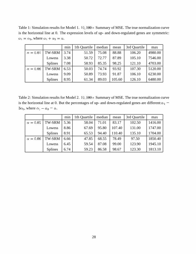
Table 1: Simulation results for Model 1.� . � . ..
�Summary of MSE. The true normalization curve
is the horizontal line at 0. The expression levels of up- and down-regulated genes are symmetric:
� � � � , where � ��� � � � .
min 1th Quartile median mean 3rd Quartile max
� ��. � .�
TW-SRM 3.74 51.59 75.08 88.88 106.20 4980.00Lowess 3.38 50.72 72.77 87.89 105.10 7546.00
Splines 7.08 58.93 85.35 98.25 121.10 4703.00
� ��. � .�
TW-SRM 6.53 50.03 74.74 93.92 107.30 5120.00Lowess 9.09 50.89 73.93 91.87 106.10 6230.00
Splines 8.95 61.34 89.03 105.60 126.10 6480.00
Table 2: Simulation results for Model 2.� . � . ..
�Summary of MSE. The true normalization curve
is the horizontal line at 0. But the percentages of up- and down-regulated genes are different: � �+�� � , where � ��� � � � .
min 1th Quartile median mean 3rd Quartile max
� ��. � .�
TW-SRM 5.36 58.04 71.01 83.17 102.50 1416.00
Lowess 8.86 67.69 95.80 107.40 131.00 1747.00Splines 8.91 65.53 94.40 110.40 135.10 1704.00
� ��. � .�
TW-SRM 6.66 47.85 68.55 78.49 97.50 1850.40Lowess 6.45 59.54 87.08 99.00 123.90 1945.10
Splines 6.74 59.23 86.58 98.67 123.30 1813.10
28
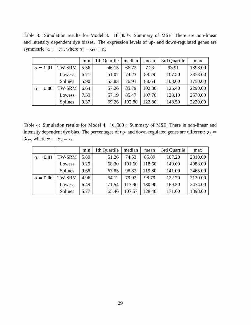
Table 3: Simulation results for Model 3.� . � . ..
�Summary of MSE. There are non-linear
and intensity dependent dye biases. The expression levels of up- and down-regulated genes are
symmetric: � � � � , where � ��� � � � .
min 1th Quartile median mean 3rd Quartile max
� ��. � .�
TW-SRM 5.56 46.15 66.72 7.23 93.91 1898.00Lowess 6.71 51.07 74.23 88.79 107.50 3353.00
Splines 5.90 53.83 76.91 88.64 108.60 1750.00
� ��. � .�
TW-SRM 6.64 57.26 85.79 102.80 126.40 2290.00
Lowess 7.39 57.19 85.47 107.70 128.10 2570.00Splines 9.37 69.26 102.80 122.80 148.50 2230.00
Table 4: Simulation results for Model 4.� . � ...
�Summary of MSE. There is non-linear and
intensity dependent dye bias. The percentages of up- and down-regulated genes are different: � �+�� � , where � ��� � � � .
min 1th Quartile median mean 3rd Quartile max
� ��. � .�
TW-SRM 5.89 51.26 74.53 85.89 107.20 2810.00Lowess 9.29 68.30 101.60 118.60 140.00 4088.00
Splines 9.68 67.85 98.82 119.80 141.00 2465.00
� ��. � .�
TW-SRM 4.96 54.12 79.92 98.79 122.70 2130.00Lowess 6.49 71.54 113.90 130.90 169.50 2474.00Splines 5.77 65.46 107.57 128.40 171.60 1898.00
29
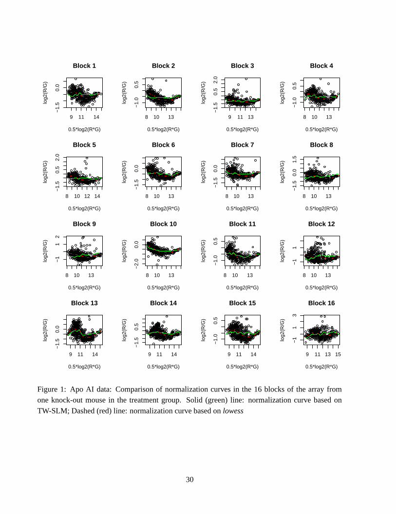
9 11 14
−1.
50.
0
Block 1
0.5*log2(R*G)
log2
(R/G
)
8 10 13
−1.
00.
5
Block 2
0.5*log2(R*G)lo
g2(R
/G)
9 11 13
−1.
50.
52.
0
Block 3
0.5*log2(R*G)
log2
(R/G
)
8 10 13
−1.
00.
5
Block 4
0.5*log2(R*G)
log2
(R/G
)
8 10 12 14
−1.
50.
52.
0
Block 5
0.5*log2(R*G)
log2
(R/G
)
8 10 13
−1.
50.
0
Block 6
0.5*log2(R*G)
log2
(R/G
)
8 10 13
−1.
50.
0
Block 7
0.5*log2(R*G)lo
g2(R
/G)
8 10 13
−1.
50.
01.
5
Block 8
0.5*log2(R*G)
log2
(R/G
)8 10 13
−1
12
Block 9
0.5*log2(R*G)
log2
(R/G
)
8 10 13
−2.
00.
0
Block 10
0.5*log2(R*G)
log2
(R/G
)
8 10 13
−1.
00.
5
Block 11
0.5*log2(R*G)
log2
(R/G
)
8 10 13
−1
1
Block 12
0.5*log2(R*G)lo
g2(R
/G)
9 11 14
−1.
50.
0
Block 13
0.5*log2(R*G)
log2
(R/G
)
9 11 14
−1.
50.
5
Block 14
0.5*log2(R*G)
log2
(R/G
)
9 11 14
−1.
00.
5
Block 15
0.5*log2(R*G)
log2
(R/G
)
9 11 13 15
−1
13
Block 16
0.5*log2(R*G)
log2
(R/G
)
Figure 1: Apo AI data: Comparison of normalization curves in the 16 blocks of the array fromone knock-out mouse in the treatment group. Solid (green) line: normalization curve based on
TW-SLM; Dashed (red) line: normalization curve based on lowess
30
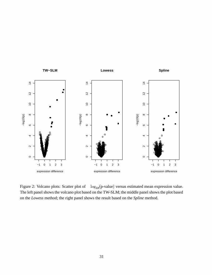
−1 0 1 2 3
02
46
810
1214
TW−SLM
expression difference
−lo
g10(
p)
−1 0 1 2 3
02
46
810
1214
Lowess
expression difference
−lo
g10(
p)
−1 0 1 2 3
02
46
810
1214
Spline
expression difference
−lo
g10(
p)
Figure 2: Volcano plots: Scatter plot of & ���� � � � p-value � versus estimated mean expression value.The left panel shows the volcano plot based on the TW-SLM; the middle panel shows the plot basedon the Lowess method; the right panel shows the result based on the Spline method.
31
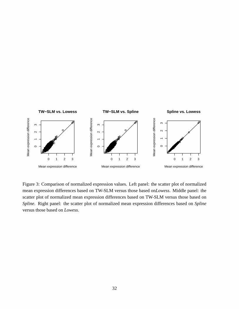
0 1 2 3
01
23
TW−SLM vs. Lowess
Mean expression difference
Mea
n ex
pres
sion
diff
eren
ce
0 1 2 3
01
23
TW−SLM vs. Spline
Mean expression difference
Mea
n ex
pres
sion
diff
eren
ce
0 1 2 30
12
3
Spline vs. Lowess
Mean expression difference
Mea
n ex
pres
sion
diff
eren
ce
Figure 3: Comparison of normalized expression values. Left panel: the scatter plot of normalizedmean expression differences based on TW-SLM versus those based onLowess. Middle panel: the
scatter plot of normalized mean expression differences based on TW-SLM versus those based onSpline. Right panel: the scatter plot of normalized mean expression differences based on Spline
versus those based on Lowess.
32
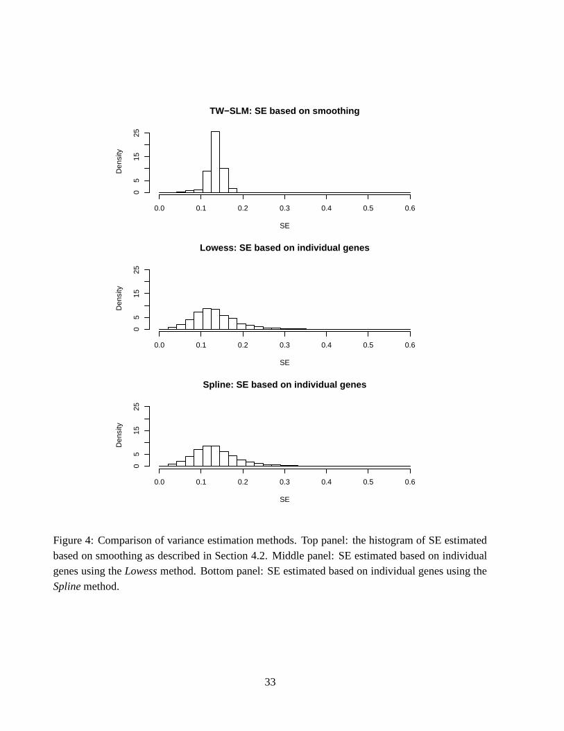
TW−SLM: SE based on smoothing
SE
Den
sity
0.0 0.1 0.2 0.3 0.4 0.5 0.6
05
1525
Lowess: SE based on individual genes
SE
Den
sity
0.0 0.1 0.2 0.3 0.4 0.5 0.6
05
1525
Spline: SE based on individual genes
SE
Den
sity
0.0 0.1 0.2 0.3 0.4 0.5 0.6
05
1525
Figure 4: Comparison of variance estimation methods. Top panel: the histogram of SE estimated
based on smoothing as described in Section 4.2. Middle panel: SE estimated based on individualgenes using the Lowess method. Bottom panel: SE estimated based on individual genes using the
Spline method.
33