Embed Size (px)
Citation preview

A Two Stage Model for Quantitative PCR
Emily Stone and John GoldesDept. of Mathematical Sciences
The University of MontanaMissoula, MT 59801
andMartha Garlick
Department of Mathematics and StatisticsUtah State UniversityLogan, UT 84322-3900
February 8, 2006
Abstract
In this paper we develop a suite of deterministic models for the reactions of quantitativePCR based on the law of mass action. The models are created by adding more reaction speciesto a base model (the logistic equation). Qualitative analysis is preformed at each stage andparameters are estimated by fitting each model to data from Roche LightCycler (TM) runs.
1

1 Introduction
The Polymerase Chain Reaction (PCR), a technique for the enzymatic amplification of specifictarget segments of DNA, has revolutionized molecular biological approaches involving genomicmaterial. This, in turn, has impacted research in human genetics, disease diagnosis, cancer de-tection, evolutionary and developmental biology, and pathogen detection, to name a few. Thecompany Idaho Technology, Inc. has capitalized on the invention of fluorescent probe techniquesto create fast, accurate devices for quantitiative PCR. Quantitative PCR is a method where theamount of amplified DNA (or amplicon) is tracked throughout the reaction and the initial amountof sample DNA can then be estimated. Understanding the important parts of a complex reactionthat is repeated tens of times, is critical in improving the design of these processes in the labora-tory, and to date theoretical studies of quantitative PCR are limited. In this paper we present asuite of deterministic models for quantitative PCR, with parameters estimated from data providedfrom Roche LightCycler (TM) PCR runs. Determining the critical features of the model throughconstruction of increasingly complex descriptions of the reaction is the overall goal of the project.
In PCR a reaction mixture containing a few copies of the target double-stranded DNA is firstheated to separate the DNA into single strands. It is then rapidly cooled and held at a lowertemperature briefly so that PCR primers (short single strands of DNA that have been designedfor this purpose) anneal specifically to the template DNA. The enzyme Taq Polymerase recognizesthese primer-template pairs and synthesizes a new strand of DNA, starting at the end of theannealed primer. In this way, a complementary strand is made from each strand of the originaldouble-stranded DNA molecule. Under ideal reaction conditions the number of copies of thisstretch of DNA in the sample is doubled in each heating-cooling cycle.
Instruments that perform real-time PCR usually detect the amplified DNA using fluorescent probesthat are added to the PCR reagents before temperature cycling. These probes bind to the DNA andgenerally fluoresce more when bound than when free. When there is a sufficient quantity of DNApresent in the sample (for example, after many temperature cycles), this change in fluorescence isdetected using a fluorimeter. If the fluorescent signal of a sample rises above a background level,a sizable amount of DNA has been synthesized, indicating that the specific DNA was initiallypresent.
Current methods for DNA quantification (for more information see the following references: Mor-rison et al. (1998), Wittwer et al. (1994, 1997), Weiss and Von Haeseler (1997), Sun (1995), Sunet al. (1996)) with PCR are based on comparing a set of successively diluted standards againstunknown samples. The methods utilize the concentrations of the standards in a dilution series todetermine the concentration of the unknown. The amount of DNA in successively diluted stan-dards is typically decreased by factors of 2 or 10, and anywhere from three to ten standards areused. Figure 1 shows a set of six standards containing between one and 1,000,000 copies of ini-tial DNA template. The fluorescence curve that crosses the threshold value at the smallest cyclenumber initially had 1,000,000 copies of DNA, the next curve to cross the threshold had 100,000copies of DNA initially, and so on. Notice that the curve that does not cross the threshold is thecontrol no template sample. Also plotted on this graph are two sets of replicates with unknowninitial quantities of DNA template.
A quick estimate of the order of magnitude of the number of copies of DNA initially in the unknownsamples can be found by simply comparing the amplification curves of the samples and diluted

0 5 10 15 20 25 30 35 40 45−1
0
1
2
3
4
5
6
7
8
9
cycle number
fluor
esce
nce
leve
l
decreasinginitial copy
number
no template
Figure 1: Fluorescence level vs. cycle number during PCR Roche Lightcycler run. Different linesare standard dilutions for quantification purposes, from 106 copies down to 101 and no templateas a control. Also run simultaneously are two samples of unknown concentration, five replicateseach.
standards. Current methods produce more precise estimates using a mathematical model of PCRthat assumes the product grows exponentially:
Cn+1 = Cn + ECn = (1 + E)Cn = (1 + E)nC0. (1)
In this model, C represents the number of copies of DNA, n represents the cycle number and Erepresents the efficiency of the PCR. E can be thought of as the percentage of existing DNA thatis replicated in a cycle. Dilution standards have known values for C0, and data from these samplescan be used to calculate the efficiency E. Given the efficiency, the initial copy number C0 can beestimated for each unknown sample.
This model is accurate for a small number of cycles, but grows less and less accurate as the numberof DNA copies grows. Unfortunately, the fluorescence signal can be distinguished from the noiseonly later in the experiment, precisely as the model becomes less accurate. The simplest mistakein the model is the assumption that the efficiency does not change with cycle number, and thatthe number of copies of DNA always grows. In reality, PCR products saturate the reaction andresources are exhausted, slowing and eventually stopping DNA synthesis.
Quantification software based on the exponential growth model uses cycle-by-cycle fluorescencemeasurements to determine a quantity known as the cycle threshold (sometimes abbreviated CT).This threshold is a measure of the smallest fractional cycle number where the fluorescence of thesample is greater than the background. CTs are difficult to determine because the backgroundfluorescence can drift up or down and the point where the fluorescence crosses the threshold isvery dependent on noise in the data. Furthermore, most existing software requires users to setthe threshold manually. The best automated method for finding CT doesn’t associate CT with a

threshold, but instead determines CT with the cycle where the second derivative of the fluorescencecurve is maximized. It is thought that this point is the cycle value where the fluorescence firstexceeds the background, i.e. by “accelerating” out of the background. However, this method hastwo potential numerical problems. First, differentiation of data is a numerically ill-conditionedproblem; and second, the data must be approximated by a continuous function to find fractionalvalues for CT. Therefore, with either the thresholding algorithm or the second derivative algorithm,it is unlikely CT can be calculated robustly. The goal of this calculation is to compute values C0,and unfortunately, even small errors in CT lead to large errors in value of C0 because PCR increasesthe number of copies exponentially.
The amplification curves suggest that a more natural model for the PCR reaction would be logistic,which proceeds to saturation as a resource is depleted. Current IT software fits the data to such alogistic map, and uses the result to estimate initial copy number of the template. For the purposeof this estimation both the exponential growth model and the logistic model are sufficient inmany cases, and have the advantage of a limited number of free parameters, requiring a minimumamount parameter estimation. However, for the long range goal of developing a more completemodel of the reaction that can lead to innovation in process design, we must look beyond theseone dimensional approximations. We also see that the data deviate from the logistic model ina consistent way for all the amplification curves, suggesting that the simplifications leading to iteliminate some critical features of the dynamics.
To our knowledge no deterministic model of the reactions of PCR that does not include assumptionsabout the kind of enzyme kinetics involved (i.e. Michaelis-Menten) are present in the literature.Stochastic models for estimating reaction efficiency and specificity can be found however, forinstance, in Sun (1995) a model for distributions of mutations and estimation of mutation ratesduring PCR is developed, using the theory of branching processes. Another such model is reportedin Weiss and Von Haeseler (1995), where the accumulation of new molecules during PCR is treatedas a randomly bifurcating tree to estimate overall error rates for the reaction. In Schnell andMendoze (1997), the reaction efficiency of quantitative competitive PCR (QC-PCR: a target anda competitor template are amplified simultaneously to provide an internal standard for identifyingthe initial target template amount) is computed using Michaelis-Menten type kinetics.
Stolvitzky and Cecchi (1996) address the validity of assuming a constant efficiency during a PCRreaction by deriving the probability of replication during successive cycles as a function of physicalparameters. In the same vein, Velikanov and Kapral (1999) report on a probabilistic model ofthe kinetics of PCR using microscopic Markov processes. The result is an exact solution for thedistribution of lengths of synthesized DNA strands, and an optimization procedure is applied todetermine control parameters that maximized the yield of the target sequence. Most recently, ina 2004 publication Whitney et al. describe a stochastic model for competitive interactions duringPCR to compute product distributions at the completion of regular PCR. The calculated yieldis compared to experimental values from the amplification of three different size amplicons, withgood results.
In the following sections we describe a hierachy of models built by including more biochemistryinto each sucessive level of approximation. We analyze qualitatively and numerically the solutionsto the models under typical operating conditions, and perform parameter estimation with dataprovided by Idaho Technology. Finally the advantages and disadvantages of including more detailsof the reactions into the model are discussed.

2 The Reactions of PCR
Table I: List of Variables and Notation Used in PCR Models
Variable name quantityC copy numberE exponential efficiency of reaction
S, s single stranded DNA (ssDNA), s = [S]P, p primer molecule, p = [P ]S′, s′ primed ssDNA, s′ = [S′]Q, q Taq molecule, q = [Q]C, c enzyme complex, c = [C]N, n nucleotide sequence for the extension, n = [N ]D, d double stranded DNA (dsDNA), d = [D]
k−1, k1 forward and backward reaction rates for annealingk−2, k2 forward and backward reaction rates for complex formationk−3, k3 forward and backward reaction rates for extension
ε logistic map growth parameterδ logistic model growth parameterK carrying capacity of the logistic map
Γ(di) growth parameter function for Taq modele, α parameters in Γ(di)Wi estimation of Γ(di) from experimental dataYi logarithmic regression variable∆t time step in discrete version of logistic modelt1 time in stage I of two stage model without Taq dynamicst2 time in stage II of two stage model without Taq dynamicsτI rescaled time in stage I of two stage model without Taq dynamicsτII rescaled time in stage II of two stage model without Taq dynamics
K, Kn,Kd, Ks conserved quantities in the two stage modelsKK normalization parameter used for experimental dataβ, γ rescaled reaction rates in the two stage model with Taq dynamics
s′I , s′II s′ in stage I and stage II respectivelyx fixed point of the x variable
tI , tII time in stage I and stage II in model with Taq dynamics
The PCR reaction proceeds through repeated cycles of dissociation, annealing and extention byTaq polymerase. During dissociation the sample is heated to approximately 90 degrees C wherethe template’s DNA nucleotide base pairs unbind and the strand essentially unzips to form twohalf-strands (single stranded DNA). The sample is then cooled to a temperature where the primerreaction is optimal (about 60 degrees C), during which primer molecules, themselves sequencesof single stranded DNA that have been designed to adhere to either end of the target sequenceof the template, bind on. Then the sample is heated again to a temperature where Taq enzymeadds base pairs on the bracketed sequence to form a new double-stranded piece of DNA. Theannealing/extension can done in one or two distinct steps, either with a continuous ramp-up tothe Taq operating temperature (during which time the primers anneal) or with a lower temperatureannealing stage followed by a higher temperature extension phase. We model the latter, but the

model itself could easily be adapted for the one-step scenario.
These three phases, dissociation, annealing, and extension are repeated typically 30-40 times toyield exponentially growing numbers of the target sequence, assuming the reaction runs as de-signed. Factors influencing the success of the reaction (is there a product?) are competition fromcontaminants in the reaction mixture, primers that bind to themselves or other primer molecules(primer-dimers), or primers that can extend pieces of the template other than the target, to namea few. Naturally the reaction saturates, see fig. 1, which is assumed to occur by complete depletionof primer molecules, since they are incorporated into the extended strands. The nucleotides inthe mixture could also be used up, but typically they are present in great numbers to preventthis from occurring. Primers are synthesized molecules and are therefore much more costly thannucleotides. Also, the initial amount of DNA to be amplified can not be either too large or toosmall. If it is too large the number of primers is not sufficient to completely prime the molecules,and if too small it can lose out to the competing amplification of undesired sequences.
The reaction equations for these phases can be written as follows.Dissociation:
D → 2S
Annealing:
S + Pk1−→←−
k−1
S′
Extension:
S′ + Qk2−→←−
k−2
C
C + Nk3−→←−
k−3
D + Q
Here D is double-stranded DNA, S is single-stranded DNA, P is primer, S′, primed single-strandedDNA, Q, Taq polymerase, C, complex of primed single-stranded DNA, P ′, and Taq, N , nucleotides.The plus/minus k’s represent the forward and backward reaction rate respectively. Ideally thereactions form a cascade, the product of one reaction continues into the next reaction and thefinal double-stranded DNA cycles back to the dissociation phase. In reality the reactions occursimultaneously, with highest frequency at their optimal temperature. For our purpose we willtreat the phases as distinct and cascade the output of one phase to the input of the next. Wealso assume that the back reactions are negligible compared to the forward reactions in all but thecreation of the enzyme complex, e.g. k−1 = k−3 = 0.
The law of mass action can be invoked to create differential equations for the concentrations ofthe above reactants, and we use lower case letters to indicate these concentrations, e.g. [S] = s,[D] = d, etc. We assume that the resource, nucleotides, is present in chunks of appropriatesequences of base pairs for the segment of DNA being extended. That is, we will assume that theextension happens all at once, not one base pair at a time. For the annealing reaction we have:
ds
dt= −k1sp (2)
dp
dt= −k1sp (3)
ds′
dt= +k1sp. (4)
And for the extension phase the equations are:
ds′
dt= −k2s
′q + k−2c (5)
dq
dt= −k2s
′q + k−2c + k3cn (6)
dc
dt= k2s
′q − k−2c− k3cn (7)
dn
dt= −k3cn (8)
dd
dt= k3cn. (9)
The exponential model (1) is a first level of approximation to the growth of double-stranded DNAcreated in these reactions, and the next level is simplification to a logistic map. This can be arrivedat in a straightforward manner from these reaction equations by first ignoring the enzyme (Taq)dynamics. Working with the set of equations that result if the Taq dynamics is ignored we have:Annealing (as above):
ds
dt= −k1sp
dp
dt= −k1sp
ds′
dt= +k1sp
Extension:ds′
dt= −k3s
′n (10)
dn
dt= −k3s
′n (11)
dd
dt= k3s
′n (12)
If the annealing stage is assumed to acheive 100% priming, the output of the first three equationsis s′ = s, the initial condition into the extension phase. In the extension phase there is a conservedquantity, namely d + n. Allowing d + n = K = d(0) + n(0) and setting n = K − d the extensionphase can be reduced to two equations:
ds′
dt= −k3s
′(K − d)
dd
dt= k3s
′(K − d).

Taking an Euler step approximation to the ODEs in the extension phase leads to:
∆s′ = −k3∆ts′(K − d)
∆d = k3∆ts′(K − d).
If the time step ∆t is taken to be the time in the extension phase the result is a map for amountsof s′, d, and n from the beginning of the extension phase to the end. For the i-th cycle:
∆s′ = s′i+1 − s′i = −εs′i(K − di)
∆d = di+1 − di = εs′i(K − di).
where ε = ∆tk3. With perfect priming s′i = si, and with perfect dissociation si = 2di, the lastequation becomes
di+1 = di + ε2di(K − di), (13)
which is a logistic map for di. The limiting factor in this derivation is the nucleotides, n, but morerealistically the primers are limiting. A similar derivation can be carried out where the extensionphase is perfect and the annealing phase is the limiting step, in which case the equation is thesame, but the limiting factor is the primer.
To test the assumption of logistic data, and we fit a dilution series from a Roche LightCycler(TM) run to (13). The run was typical for these quantification experiments: it had 45 cycles,each consisting of a brief melt stage at 95 degrees C, a 10 second annealing stage at 55 degrees C,and a 30 second extension stage at 72 degrees C. The fluorescence aquisition occurred at the endof the annealing stage, and used a FRET (fluorescence resonance energy transfer) probe system.FRET probes are a pair of oglionucleotides labeled with fluorescent dyes. The pair are designedto hybridize to adjacent regions on the target DNA, and the marker dyes of each probe can onlyinteract when they are in close proximity and bound to the target. The fluorophores are chosen sothat the emission spectrum of one overlaps with the excitation spectrum of the other. The donorfluorophore is excited by a light source, transfers its energy to an acceptor fluorophore, which thenemits light of a longer wavelength. This light is then detected during the fluorescence acquisition.
The parameter estimation was done in MATLAB using least squares to first compute K and γ,and a simplex search method based scheme (MATLAB’s fminsearch) to find the initial fluorescencelevel. The objective function used in the nonlinear optimization was the two-norm of the differencebetween the model time series and the data. Percentage error was computed by dividing the finalvalue of the objective function by the two-norm of the model time series.
Table II: Parameter Estimation for the Logistic Model (13)
γ K d0 % errorrun 1 0.0185 8.1473 2.9× 10⁻² 5.15run 2 0.0189 8.2832 1.6× 10⁻² 5.8run 3 0.0214 7.9001 4.2× 10⁻³ 5.15run 4 0.0296 6.678 5.5× 10⁻⁴ 4.9run 5 0.0457 4.5959 1.02× 10⁻⁵ 5.3run 6 0.1273 1.5445 4.12× 10⁻⁵ 5.82

The results of the parameter estimation for the dilution series are present in figure 3 and TableII. We see that the model is more than adequate for predicting initial copy number, given thecurrent practice of running standards simultaneously with samples to generate a map betweeninitial copy number and fluorescence level. The drift in the growth constant for decreasing copynumber indicates that some aspect of the dynamics is not captured by this map, and for thelowest copy number run (number 6) we see that the initial amount estimated is off by an orderof magnitude. In this case competition from other reactions is thought to be the culprit, but inall cases the map is a gross simplification to the actual dynamics. It clearly overestimates thegrowth for earlier cycles, and approaches saturation more quickly at later cycles. To verify thisintuition quantitatively we preformed a version of logarithmic regression on the first five runs of thedilutions series (see figure 2). The basis for this regression is the separation of variables solutionto the logistic differential equation:
dy
dt= δy(K − y),
namelyln(
y
K − y) = Kδt + ln(
y0
K − y0).
If y follows logarithmic growth the variable Y = ln( yK−y ) will depend linearly on time t. Plots of
the discretely sampled variable Yi vs. cycle number i for standard data set are shown in figure 4,where it is obvious that they are not well-estimated by a linear function of i. There are severalstraight line regions in these graphs, corresponding to a) low cycle number noise, b) a region wherethe initial exponential growth occurs, and c) a third region where saturation happens, with a slopeless than that seen in the second region. A linear fit of this data would have an intermediate slopecausing an overestimate or an underestimate of the data, depending on the cycle number. Thisis apparent in figure 3, where it also is clear that the data approach the saturation level moreslowly than logistic growth would warrant. One explanation of this is reduced efficiency of Taqpolymerase when the quantity of molecules to extend becomes very large. This suggests a growthparameter Γ(di) that varies with the amount of amplicon, d, so that
di+1 = di + Γ(di)di(K − di),
where Γ(di) is a decreasing function of di. The shape of this function can be estimated by plottingthe variable found by solving the above equation for Γ:
Wi =di+1 − di
di(K − di)= Γ(di).
That is, the graph of Wi vs. di will give an idea of Γ(di). An example is shown in figure 5. Thefunction Γ appears to be inversely proportional to di, so we fit a new map with Γ(di) = e
1+αdi, so
di+1 = di +edi
1 + αdi(K − di). (14)
The results are shown in figure 6, and in Table III. The error presented there is the mean squareerror.
Table III: Parameter Estimation of Taq Model (14).

0 5 10 15 20 25 30 35 40 45−1
0
1
2
3
4
5
6
7
8
9
cycle number
fluor
esce
nce
leve
l
decreasinginitial copy
number
no template
Figure 2: Fluorescence amplification data from an Roche Light-Cycler run. Five standard dilutionseries
0 5 10 15 20 25 30 35 40−1
0
1
2
3
4
5
6
7
8
9
cycle number
fluor
esce
nce
leve
l
Figure 3: Fitting dilution series data with a logistic map. See text for parameter values. Solidline- model, (+++++)- data.

5 10 15 20 25 30 35 40 45−10
−8
−6
−4
−2
0
2
4
cycle number i
Yi
Figure 4: Logarithmic regression curves for five standard dilution series.
1 2 3 4 5 6 70
0.02
0.04
0.06
0.08
0.1
0.12
di
Wi
Figure 5: Plotting Wi vs. di to estimate Γ(di) for the first four dilution series runs.

0 5 10 15 20 25 30 35 40 45
0
2
4
6
8
10
cycle number
fluor
esce
nce
leve
l
0 5 10 15 20 25 30 35 40 45
0
2
4
6
8
10
cycle number
fluor
esce
nce
leve
l
decreasinginitial copynumber
sample 1
sample 2
Figure 6: Standards data fitted with the Taq model (14). See Table II for parameter and errorinformation.

error e K α d0
run 1 0.1894 0.1481 8.5579 0.9148 4.91× 10⁻⁷
run 2 0.2055 0.1473 8.7559 0.8907 7.31× 10⁻⁸
run 3 0.2587 0.1227 8.3295 0.6096 1.20× 10⁻⁷
run 4 0.3639 0.1237 6.9411 0.4158 1.06× 10⁻⁷
run 5 0.3945 0.1592 4.7559 0.4111 7.53× 10⁻⁸
run 6 0.2394 0.3721 1.5740 0.6636 3.02× 10⁻⁷
sample 1a 0.2321 0.1413 9.3277 0.5918 3.98× 10⁻⁸
sample 1b 0.2377 0.1546 9.5827 0.7381 1.04× 10⁻⁸
sample 1c 0.2189 0.1231 9.7042 0.5957 1.57× 10⁻⁷
sample 1d 0.2582 0.1202 9.9448 0.6035 1.60× 10⁻⁷
sample 1e 0.2610 0.1196 10.0509 0.6391 1.62× 10⁻⁷
sample 2a 0.4427 0.1297 6.5511 0.3543 8.28× 10⁻⁸
sample 2b 0.4203 0.1222 6.8775 0.3390 9.03× 10⁻⁸
sample 2c 0.4328 0.1214 6.9499 0.3581 9.08× 10⁻⁸
sample 2d 0.4223 0.1173 7.1260 0.3541 1.07× 10⁻⁸
sample 2e 0.4270 0.1267 6.9205 0.3514 6.42× 10⁻⁸
The growth coefficient for this model (e), and the value for α are more consistent than for theregular logistic model, though the variation is more pronounced in smaller copy number runs, andsuffers the same overcalculation of the initial fluorescence in run 6. (Also in run 6 the modelcoefficients are significantly different from the other runs). We also fitted the replicates of theunknown samples with reasonably consistent results, though it is clear there is a trade-off betweenvalues such as the growth constant e and the initial fluorescence, indicating hidden dependenciesin the parameters that cannot be differentiated with this sort of data.
This could be the end of the story, but an empirically determined rate function is not as satisfactoryas a model that captures the behavior built-up directly from the reaction equations. In the nextsection we construct such a model and parameterize it with the data.
3 The Two Stage Model
We consider here two versions of a two stage model, one that includes the dynamics of the Taqenzyme, and one that does not. The latter is much simpler and can be solved analytically, so wepresent it first. Both make the assumption of complete dissociation, so that the amount of ssDNAentering the annealing phase is equal to twice the amount of dsDNA from the previous extensionphase, plus whatever ssDNA was leftover from the previous annealing phase. This eliminatesthe need for the equation that describes dissociation (or the “melt”) phase of the reaction. Wenext assume that the annealing phase happens distinct from the extension phase and call thisstage I. The equations for stage I are (2)-(4). The extension phase we name stage II, and withTaq dynamics the equations are (5)-(9). Without the Taq dynamics the equations are given by(10)-(12).
3.1 Two Stage Model without Taq Dynamics
The two stages in both versions are linked through their initial conditions, and in both the initialamount of primed ssDNA in stage II is equal to the amount created in stage I, while the initialamount of nucleotide in stage II is whatever was left over from the previous cycle of stage II. Forthe model without Taq dynamics, upon completion of stage II any unextended primed ssDNA willbreak-up in dissociation, and thus the initial amount of ssDNA in stage I is that plus the amountleft-over from the previous stage I, plus twice the amount of double stranded DNA created in stageII. The initial amount of primer in stage I is also the sum of the dissociated amount from stageII and the amount leftover from the previous stage I. The initial amount of double-stranded DNAin stage II is assumed to be zero at the start of every cycle. Written as equations these initialconditions are:
Stage I:
s(0) = s(tend, previous stage I) + s′(tend, previous stage II) + 2d(tend,previous stage II); (15)
p(0) = s′(tend, previous stage II) + p(tend, previous stage I); s′(0) = 0.0; (16)
Stage II:
s′(0) = s′(tend, stage I); n(0) = n(tend, previous stage II); d(0) = 0.0. (17)
There are two conserved quantities in the equations for both stage I and stage II, so the systemscan be reduced to one equation each and solved analytically. For stage I we use the conservedquantities: p(t) − s(t) = K = p(0) − s(0) and s(t) + s′(t) = Ks = s(0) − s′(0) = s(0), (sinces′(0) = 0) so that the resulting ODE for p(t) is
dp
dt= k1(K − p)p,
with the solutionp(t) =
K
1− s(0)p(0) exp(−Kk1t)
.
and the other variables are found from the conserved quantities:
s(t) = p(t)−K = p(t)− p(0) + s(0),
s′(t) = Ks − s(t) = s(0)− s(t).
It is expedient to rescale the dependent variables in the original ODEs by the amount of onequantity at the beginning of the reaction, and since the nucleotides are present in excess we callthat N0 and define new variables: p = p
N0, s = s
N0, s′ = s′
N0, n = n
N0, d = d
N0. We also rescale time
by define a new time t1 = k1t, where k1 = k1N0.
The solution is then
p(t1) =K
1− s(0)p(0) exp(−Kt1)
,
s(t1) = p(t1)− K = p(t1)− p(0) + s(0),

s′(t1) = Ks − s(t1) = s(0)− s(t1).
where K = p(0)− s(0), Ks = s(0).
The quantities in stage II can be computed in an identical manner, and with the choice of conservedquantities s′(t) + d(t) = Kd = s′(0) + d(0) = s′(0), n(t)− s′(t) = Kn = n(0)− s′(0) the solution is
n(t) =Kn
1− s′(0)n(0) exp(−Knk2t)
,
and the other variables are found from the conserved quantities:
s′(t) = n(t)−Kn = n(t)− n(0) + s′(0),
d(t) = Kd − s′(t) = s′(0)− (n(t)− n(0) + s′(0)) = n(0)− n(t).
Rescaling again by the amount of nucleotide at the beginning of the first cycle, N0, and definingt2 = k2t, (where k2 = k2N0) results in
n(t2) =Kn
1− s′(0)n(0) exp(−Knt2)
s′(t2) = n(t2)− Kn = n(t2)− n(0) + s′(0)
d(t2) = Kd − s′(t2) = n(0)− n(t2)
where Kd = s′(0), Kn = n(0)− s′(0). The initial conditions can be written in terms of the rescaledvariables, they are identical in form to (16) and (17), with X replacing X, for each variable. Fromthis point forward we rename X = X to simplify the notation, while keeping in mind how therescaling changes the initial conditions.
A map from one cycle to the next can be constructed from these solutions and the initial conditions(16) and (17). To distinguish between the concentration of primed single stranded DNA (ssDNA’)in the first and second stage we designate them s′I and s′II . Let the final time for each stage befixed at τI and τII respectively. The map for stage I is then:
pi(τI) =Ki
1− si(0)pi(0) exp(−KiτI)
,
where Ki = pi(0)− si(0), and
si(τI) = pi(τI)−K = pi(τI)− pi(0) + si(0),
s′Ii (τI) = Ks − si(τI) = si(0)− si(τI),
and for stage II:
ni(τII) =Kn
1− s′IIi (0)ni(0) exp(−KnτII)
,
where Kn = ni(0)− s′IIi (0), and
s′i(τII) = ni(τII)−Kn = ni(τII)− ni(0),

di(τII) = Kd − s′IIi (τII) = ni(0)− ni(τII).
The initial conditions for the ith cycle are:
si(0) = si−1(τI) + s′IIi−1(τII) + 2di−1(τII),
pi(0) = pi−1(τI) + s′II(τII),
s′I(0) = 0.0,
s′IIi (0) = s′Ii (τI),
ni(0) = ni−1(τII),
di(0) = 0.0.
While a closed form version of the map can be written down, it is not particularly illuminating,simulations must be performed to uncover the behavior of the solutions. To do this parametersmust be estimated or fit from the data, these are τI , τII , and the initial concentrations of primerand ssDNA, p1(0), s1(0), relative to the initial concentration of nucleotides, N0. The model anddata must both saturate at the same level, and a scaling quantity for the data values was fit foreach curve, which we called KK. The parameter estimation was done as in the previous section,with the same set of data. The percentage error in each fit was computed by dividing the finalvalue of the objective function by the two-norm of the model time series vector.
For the dilution series all these parameters were fit, see figure 7 and Table IVa. The KK valuefound is consistent with the variation of the saturation value for each run, and the for each run τ1
is greater than τ2, indicating that annealing is slower than extension. The initial quantity s1(0)decreases roughly by a factor of 10 for each run, also consistent with the dilution series. Theinitial amount of primer in each run is close to 1.0, indicating the amount of primer must beclose to the amount of nucleotide in a run to match the data, which is not consistent with theinformation we have about the experiment, which is that the nucleotides (measured in blocks ofthe template sequence to be amplified) to primer ratio is about 4-to-1. We return to this issuewhen we examine the model including Taq dynamics. The 6th run has a much larger error thanthe others, indicating that other factors come into play in the dynamics of very small copy numberruns, such as competition from other species (e.g. primer-dimers).
We then fit the model to the runs with unknown initial concentrations, of which there are two,each with five replicates. For the these 10 runs τI , τII , p1(0) were fixed at values from the dilutionrun nearest in CT (for the sample 1 this was run 2, for sample 2, run 4). The results from thisexercise are presented in Table IVb.
Table IVa: Parameter Estimation of the Two Stage Model without Taq Dynamics-Dilution Series
KK τI τII s1(0) p1(0) % errorrun 1 8.989 1.525 0.829 1.84e-04 0.9935 10.1run 2 9.169 1.551 0.853 7.23e-05 0.9933 9.8run 3 8.768 1.597 0.916 1.67e-05 0.9930 9.4run 4 7.390 1.466 1.216 1.70e-06 0.9978 8.0run 5 4.902 1.454 1.598 1.68e-07 0.9636 10.4run 6 1.645 4.787 0.939 8.00e-8 0.991 19.38

5 10 15 20 25 30 35 40 45−0.1
0
0.1
0.2
0.3
0.4
0.5
0.6
0.7
0.8
0.9
cycle number
ampl
ifica
tion
leve
l
decreasing s0
Figure 7: Fitting dilution series data to the two stage model without Taq dynamics. For parametervalues see Table IVa.
Table IVb: Parameter Estimation of Two Stage Model w/out Taq Dyn.-Unknown Sampless1(0) KK % error
sample 1a 8.019e-05 10.35 14.7sample 1b 7.87e-05 10.482 13.0sample 1c 7.67e-05 10.518 11.2sample 1d 7.57e-05 10.713 10.9sample 1e 7.42e-05 10.722 10.7sample 2a 1.51e-06 7.158 9.4sample 2b 1.40e-06 7.490 8.6sample 2c 1.40e-06 7.518 8.6sample 2d 1.39e-06 7.688 8.5sample 2e 1.50e-06 7.430 8.8
3.2 Two Stage Model with Taq Dynamics
For this model the equations for stage I remain as (2)-(4), while the stage II equations now includeboth Taq and complex concentrations and are given by (10)-(12). As in the simpler model theinitial amount of primed ssDNA in stage II is equal to the amount created in stage I, while theinitial amount of nucleotide in stage II is whatever was left over from the previous cycle of stageII. Upon completion of stage II any unextended complex will break-up during dissociation, as willany primed ssDNA. Thus the initial amount of complex in stage II will be zero, and the amountof Taq enzyme will be the original amount from the beginning of the PCR reaction (Q). Stage

I starts with no primed ssDNA, it is assumed to dissociate during the melt phase. The primerinitial condition is the amount of unused primer from the previous cycle, plus the amount createdduring the dissociation of the complex during the melt phase. The initial amount of ssDNA willbe that left from the previous annealing phase plus an amount equal to amount of complex left instage II that dissociates, plus the ssDNA that results from the dissociation of the dsDNA createdin the previous stage II, which is double the amount of dsDNA. In terms of equations these initialconditions can be stated:
s′(0) = s′(tend, stage I); q(0) = Q; c(0) = 0.0; n(0) = n(tend,previous stage II); d(0) = 0.0.(18)
and for stage I:
s(0) = s(tend,previous stage I) + c(tend, previous stage II) + 2d(tend, previous stage II); (19)
p(0) = c(tend, previous stage II) + s′(tend,previous stage II) + p(tend, previous stage I);
s′(0) = 0.0.
A map for the reaction is created by integrating the ODEs in each stage and using the initialcondition rules to link one stage to the other. However, insight can be gained by analyzing thedynamics of each stage separately and forming some special limiting cases for this map.
3.2.1 Dynamics of Stage I
The equations for stage I are again completely integrable, because of two conserved quantities,s + s′ = Ks = s′(0) + s(0) = s(0), and p − s = K = p(0) − s(0). Simplifying the equation for pusing these quantities yields
dp
dt= k1(K − p)p. (20)
Rescaling time, t = p(0)k1t,dpdt
= p, and the molecular concentration of all three quantities by
p(0), i.e. p = pp(0) , s = s
p(0) , s′ = s′
p(0) , and K = p(0)−s(0)p(0) = 1− s(0), results in
˙p = (K − p)p,
which has the solution
p(t) =K
1− s(0)e−Kt, (21)
so the remaining quantities can be computed
s(t) = p(t)− K = p(t) + s(0)− 1,
ands′(t) = Ks − s(t) = 1− p(t).
Note that in the limit as t → ∞, p(t) → K if K > 0, e.g. 1 > s(0), more initial primer thanssDNA, and p(t) → 0 if K < 0, i.e., there is more ssDNA to begin with than primer. There is atranscritical bifurcation at K = 0, s(0) = 1, where the two fixed points for the system (20), p = Kand p = 0, exchange stability.

3.2.2 Dynamics of Stage II
The stage II ODEs can be simplified by rescaling time to remove one rate constant. The dimen-sionless time chosen, τ , is k−2t and the new system is
s′ = −γs′q + c (22)
q = −γs′q + c + βcn (23)
c = γs′q − c− βcn (24)
n = −βcn (25)
d = βcn (26)
where dfdτ = f , β = k3
k−2, γ = k2
k−2.
The initial conditions are (as stated previously):
s′(0) = s′(tend, stage I); q(0) = Q; c(0) = 0.0; n(0) = n(tend, previous stage II), d(0) = 0.0.
The molecular quantities in the above equations can themselves be scaled, we choose here to scaleby the initial amount of nucleotides available at the start of the cycle, N0 = n(0). The rescaledequations have the same form, with rescaled parameters γ = γ/N0 and β = β/N0 (meaning weadopt the notation X = X
N0for each quantity, and then discard the hat for simplicity). The
corresponding initial conditions are
s′(0) =s′(tend, stage I)
N0; q(0) =
Q
N0; c(0) = 0.0; n(0) = 1, d(0) = 0.0.
The equations (22)-(26), have three conserved quantities (e.g. n+d, q+c, s+c+d), so the dynamicscan be reduced from a five to a two-dimensional system. Since initially there will be no c or d, thethese conserved quantities can be written s′ + c + d = s′(0), q + c = q(0), n + d = 1. The twodimensional system that results from incorporating the conserved quantities is:
q = −γ(s′(0)− q(0)− 1 + q + n)q + q(0)− q + β(q(0)− q)n
n = −β(q(0)− q)n.
From this we can more readily determine fixed points and analyze their stability. Two of the threefixed points for this system are physically relevant, and are given by
f.p. 1 = (s′ = 0, q = q(0), c = 0, n = 1− s′(0), d = s′(0)).
and
f.p. 2 = (q =12γ
(γ(q(0) + 1− s′(0))− 1 +√
(−γ(q(0) + 1− s′(0)) + 1)2 + 4γq(0))),
s′ = s′(0)− q(0)− 1 + q, c = q(0)− q, n = 0, d = 1).
The third fixed point has the q-coordinate:
q =12γ
(γ(q(0) + 1− s′(0))− 1−√
(−γ(q(0) + 1− s′(0)) + 1)2 + 4γq(0)))

which can be shown to be always negative, and so physically irrelevant. For a proof of this fact,and the complete stability analysis, see appendix I. Here we state the main result only: There is atranscritical bifurcation when s′(0) = 1 = n(0), here f.p. 1 and f.p. 2 are identical and exchangestability. For n(0) > s′(0) f.p. 1 is attracting and has non-negative coordinate values. Forn(0) > s′(0) f.p. 2 is attracting with non-negative coordinate values. The reaction will typicallybegin with more nucleotides than primed ssDNA, so the long-time behavior is represented by f.p.1, which has final dsDNA value equal to the amount of primed ssDNA (all primed ssDNA isextended). If the initial amount of primed ssDNA exceeds the amount nucleotide at the start ofthat cycle, the second fixed point becomes attracting and non-negative, and in this case the longterm dsDNA amount will be equal to the initial amount of nucleotide. Hence the limiting valueof dsDNA switches from the initial amount of primed ssDNA to the initial amount of nucleotideas primer becomes limiting, as would be anticipated.
3.3 Limiting Cases
Assuming both stage I and stage II ODEs reach steady state, a map can be constructed by linkingthe attracting fixed points through the initial conditions. Since the rescaling of each stage used inthe previous subsection is different, (and changes with each cycle) it is best to return to the unscaledquantities to create the map. The fixed points for stage II in terms of the unscaled quantities arethe same, with the 1.0’s replaced by n(0)’s. The bifurcation occurs when s′(0) = n(0), as wasoutlined previously.
The attracting fixed point for stage I depends on the initial values of primer and ssDNA, we willwrite it (p, s, sII = p(0) − s(0), 0, s(0)) if p(0) > s(0) (there is enough primer to prime all thessDNA). If p(0) < s(0) it is (p, s, s′II = 0, p(0)− s(0), p(0)): the limiting amount is primer. Theattracting fixed point for stage II depends on the relative size of n(0) and s′(0), the latter beingequal to s′ from the previous stage I. The initial amount of nucleotide will be determined by howmuch remains from the previous cycle. In a similar manner the rest of the initial conditions aredetermined by the fixed points from the previous cycle, this dependance is detailed below.
For stage I the initial amount of primer is the sum of what is left over from the previous stage I(cycle i − 1), and the primer released from the dissociation of the complex and the unextendedprimed ssDNA from the previous stage II:
pi(0) = pi−1 + ci−1 + s′IIi−1.
The initial amount of ssDNA will be twice the amount of dsDNA created in the previous cycle,plus the ssDNA released from the dissociation of the complex and the unextended primed ssDNAfrom the previous stage II, plus the amount of ssDNA not primed in the previous stage I:
si(0) = 2di−1 + ci−1 + s′IIi−1 + si−1.
At the start of stage I there is no primed ssDNA: s′Ii (0) = 0.
In stage II the initial amount of primed ssDNA is equal to the amount coming out of stage I, s′Ii ,the initial amount of Taq is a constant, Q, the complex has been completely dissociated duringthe melt phase, along with any dsDNA. The amount of nucleotide is equal to the amount left overfrom the previous stage II:
s′II(0) = s′Ii ; qi(0) = Q; ci(0) = 0.0; ni(0) = ni−1; di(0) = 0.0.

There will be four distinct cases of the map depending on the relative size of n(0), s′II(0) andp(0), s(0). Here we limit the analysis to a physically realistic scenario: initially both primer andnucleotide dominate, but initial primer amount is less than initial nucleotide amount. In the courseof creating new amplicon both primer and nucleotide amounts decrease, and since they are used inthe same proportion the primers will be exhausted before the nucleotides. This will cause a shiftto another case of the map, and the remaining two iterations will complete the process, since nomore primer will be available to make the extension possible. The equations for this scenario arepresented next.
First assume pi(0) > si(0) and ni(0) > s− I ′II(0), so the stage I fixed point is (for the ith cycle)
pi = p(0)i − s(0)i; si = 0; s′Ii = si(0).
Then assume ni(0) > s′IIi (0) so that the fixed point for stage II is
s′IIi = ci = 0, qi = q(0).
ni = n(0)i − s′IIi (0),
di = s′IIi (0).
Now, the initial conditions for cycle i are determined by the fixed points from cycle i − 1 in thismanner:
p(0)i = pi−1 + ci−1 + s′IIi−1 = pi−1
s(0)i = 2di−1 + ci−1 + s′IIi−1 + si−1 = 2di−1.
Substituting these into the fixed point for stage I yields:
pi = pi−1 − 2di−1; si = 0; s′I = 2di−1.
The initial conditions for stage II in terms of fixed points for the previous cycle are
n(0)i = ni−1; s′II(0)i = s′Ii = 2di−1.
And so the stage II fixed point is then
s′IIi = ci = 0, qi = Q
ni = ni−1 − 2di−1
di = 2di−1
This is simple doubling of the double-stranded DNA, and will proceed until the amount of primer(p(0)) at the beginning of stage I is less than the amount of single-stranded DNA (s(0)). At thiscycle (call it N) the attracting fixed point switches in stage I and a new map is created that isvalid for exactly one cycle. The new stage I fixed point is:
pN = 0
sN = sN (0)− pN (0) = 2dN−1 − pN−1
s′IN = pN (0) = pN−1

In stage II the amount of nucleotide is depleted by an amount equal to the amount of s′I created,which equals pN−1. The amount of double stranded DNA will be equal to that amount as well, sothe map for stage II is:
s′IIN = cN = 0, qN = q(0)
nN = nN−1 − pN−1
dN = pN−1
For the next cycle, N + 1, there is no primer left so the duplication ends. The fixed point valuesin this cycle are:
pN+1 = 0
sN+1 = 2dN + sN = 2pN−1 + 2dN−1 − pN−1 = pN−1 + 2dN−1 = sfinal
s′IN+1 = 0.
For stage II:nN+1 = nN − pN = nN−1 − pN−1 = nfinal
dN+1 = 0
It is straight-forward to show that this is a fixed point for the map from one cycle to the next,once this stage is reached the final value of extended DNA is fixed. It lives in the reaction as singlestranded DNA until the mixture is allowed to “finish off” and the strands reanneal (finishing offmore technically refers to the stage in which the extension is allowed to run to completion, and allthe primed single-stranded DNA molecules have been turned into double stranded DNA, whichhappens in cycle N).
This map, created for the limiting case of infinite time for each stage in each cycle, converges onthe model of simple doubling until the reaction limiting species (either p or n) is exhausted. Thenin one cycle the reaction finishes off and reaches a fixed point. Clearly this does not capture thesigmoidal growth curve or the variation away from it. The next step is to allow the extension instage II to reach the asymptotic fixed point determined by initial conditions for each cycle, but touse the exact solution of the stage I equations, with the run time left as a parameter, to determinethe values at the end of stage I. We construct this map next.
The exact solution for the stage I variables is as follows:
pi(TI) =K
1 + si(0)pi(0)e
−KTI
= fTI(pi(0), si(0)), (27)
where K = pi(0) − si(0). The unprimed and primed ssDNA depend on p through the conservedquantities:
si(TI) = pi(TI) + si(0)− pi(0) (28)
s′Ii = pi(0)− pi(TI). (29)
The stage II fixed point for n(0) > s′II(0) > 0 will be:
s′IIi = ci = 0, qi = Q
ni = ni(0)− s′IIi (0) = ni(0)− s′Ii (TI)
di = s′II(0) = s′Ii (TI) = pi(0)− pi(TI).

The initial conditions for the next stage I are then
pi+1(0) = pi(TI) + ci + s′IIi = pi(TI), (30)
si+1(0) = 2di + ci + s′IIi + si(TI) = 2(pi(0)−pi(TI))+pi(TI)+ si(0)−pi(0) = pi(0)−pi(TI)+ si(0),
(31)and
s′i+1(0) = 0. (32)
Note that at this point the stage I initial conditions, in which the map is cast, depend only on theprevious stage I values, the stage I map runs independently of stage II. The stage II fixed pointcan be determined directly from the stage I variables, and the only one of interest is the amountof nucleotide, for when that is exhausted the reaction will stop. The equation for nucleotide, n, is:
ni+1(0) = ni = ni(0)− s′Ii (TI) = ni(0)− (pi(0)− pi(TI)). (33)
There are two possibilities for the completion of the reaction: either primer runs out or thenucleotides. In the case that primer runs out first, we look at the limit as pi(0) → 0, so thatpi(Ti) → 0 and si(TI) → si(0) and s′i(TI) → 0. In stage II no complex will be formed, ordouble-stranded DNA created, as there is no primed ssDNA available at the start of the reaction:s′IIi (0) = s′i(TI) = 0. The fixed point for the nucleotide is thus the value of the nucleotide at
the beginning of the cycle, ni = ni(0) − s′Ii (TI) = ni(0), and the map for ni is at a fixed point,ni+1(0) = ni(0).
If the resource is the limiting factor, rather than primer, in the second to last cycle ((r− 1)-cycle)we have nr−1(0) < s′II
r−1(0). This sends stage II variables to f.p. 2. In the final stage I the initialconditions are then
pr(0) = pr−1(TI) + cr−1 + s′IIr−1
sr(0) = 2dr−1 + cr−1 + s′IIr−1 + sr−1(TI),
with f.p. 2 values. At the end of stage I the function values are:
pr(TI) = fTI; sr(TI) = fTI
+ sr(0)− pr(0); s′Ir (TI) = pr(0)− fTI.
The initial condition for s′IIr (0) = s′Ir (TI) = pr(0) − fTI
, but only complex can be formed in thefinal stage II, since the resources have been exhausted, nr(0) = 0. During the dissociation phasethe complex breaks up, and the initial quantities for stage I are pr+1(0) = pr(0); sr+1(0) = sr(0).The reaction has reached a fixed point with (p = pr(0), s = sr(0), n = 0).
To illustrate the dynamics of this map we plot ni, si and pi in figure 8, called Ni, Si and Pi
in the figure caption. Six runs were performed with varying stage I integration time: (tI =0.5, 0.75, 1.0, 1.5, 2.0). The initial conditions are n0 = 1.0; p0 = 0.25; s0 = 0.001, i.e., the case inwhich primer is limiting. To further analyze the effect of varying integration time we plot thelogarithmic regression of s, the quantity Yi = ln(| si
p0−si|), in figure 9. Here we see that in the limit
of shorter integration times the growth is more nearly logistic, and for longer integration times itdeviates from logistic by being concave up, rather than concave down, as seen in the amplificationdata (figure 4). Including variation in stage I integration time is clearly not enough to capturethe correct non-sigmoidal behavior of the growth curves, some other part of the reaction dynamicsmust explain the accentuated slowing of growth during the latter half of the reaction. This leadsus to integrating and fitting parameters on the full model, eq.s (2)-(4), and (5)-(9).

0 5 10 15 20 25 30 35 40 450
0.1
0.2
p i
0 5 10 15 20 25 30 35 40 450
0.1
0.2
s i
0 5 10 15 20 25 30 35 40 450.7
0.8
0.9
cycle number i
n i
Figure 8: Integration of map with varying stage I integration time. Arrows point in the directionof decreasing stage I integration time.
0 5 10 15 20 25 30 35 40 45−5.5
−5
−4.5
−4
−3.5
−3
−2.5
−2
−1.5
−1
−0.5
0
cycle number i
Yi
increasing stage I integration time
Figure 9: Logarithmic regression variable Yn from the two-stage map with varying stage I integra-tion time.
3.4 Parameterizing the Full Two Stage Model with PCR Data
We now investigate the parameterization of the model with arbitrary time in stage I and in stage II.The reactions in the annealing phase (stage I) are the same those presented in equations (20),(21),and the linking initial conditions are (19). The stage II ODEs are given in equations (22)-(26)with rescaled parameters and initial conditions:
s′(0) =s′(tend, stage I)
N0; q(0) =
Q
N0; c(0) = 0.0; n(0) = 1.0, d(0) = 0.0.
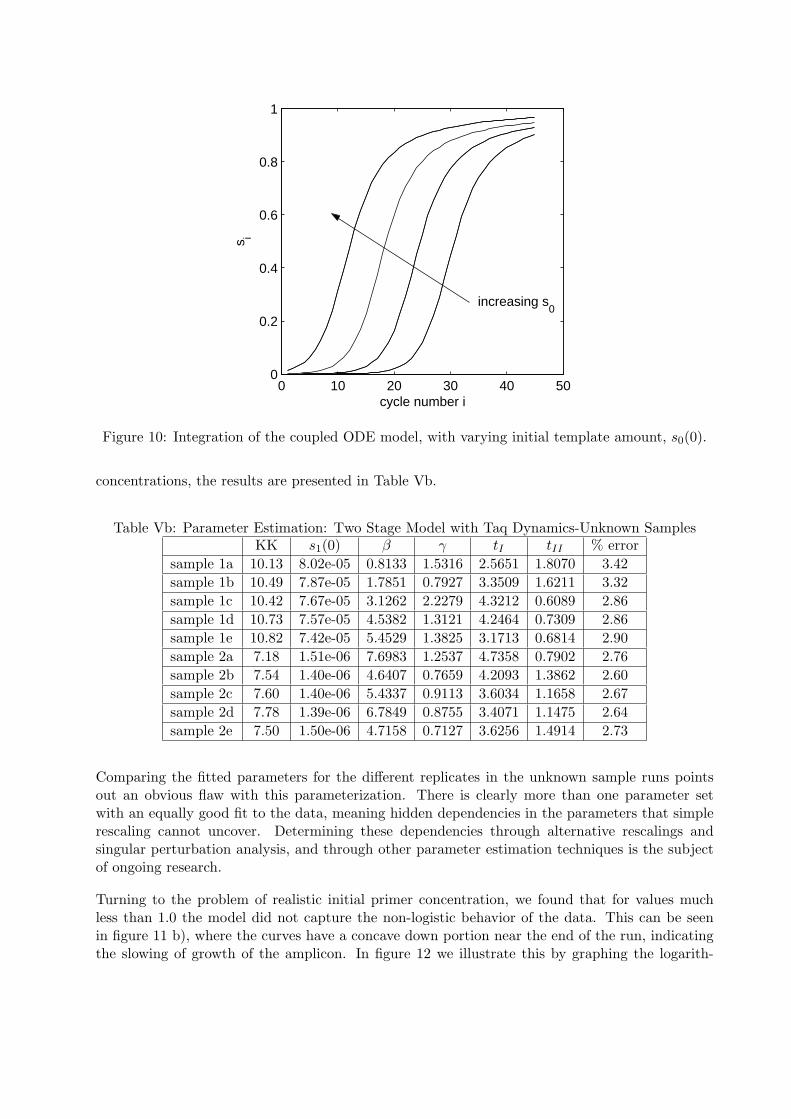
Integrating the complete model occurs in phases, first computing the solution of stage I: eqs. (21),then the value of the stage I variables at TI are used as initial conditions (18) for the stage IIintegration: (5)-(9). The following dissociation phase breaks up existing complex into ssDNA,primer and Taq, and dsDNA into twice as many ssDNA strands, and these are used as initialconditions for the next stage I (see (19)). Examples of runs with varying amounts of initialtemplate are shown in figure 10.
The parameter estimation was done using the same quantitative PCR data set in the previoussections, again using the Matlab function fminsearch to minimize the mean square error betweenthe amplification data and the simulated time series. In performing the parameterization we usedthe value determined for the initial s level from fitting the two stage model without Taq dynamics.We fit the normalization constant for the data, KK, the two reaction coefficients, β and γ, andthe reaction times tI and tII . That leaves the initial amount of primer, p1(0), and of taq, Q,relative to the initial amount of nucleotides. From the results of many parameterization runs wedetermined that the best fit was obtained when p1(0) = 1.0, which is not what is indicated by ITprotocol, where a standard reaction set-up has 0.5 micromole of each primer and 0.8 millimole ofdNTPs, the base pairs (BP) used in extension. Given an amplicon of 200 BPs this means about4 micromole of completed segments, or 2 micromole of each complementary segment. The ratioof primers to nucleotides is about four to one, then, so we should set the initial primer amountto 0.25. This never achieved the same goodness-of-fit that the runs with higher initial amountsof primer did. On the other hand, the parameterization was relatively insensitive to the initialamount of Taq polymerase, which we set at 1.0. See Tables Va,b for the parameterization results.
In figure 11 a) we show a comparison of data to model with parameters found by the algorithm,for the dilution series. The logarithmic regression variable, Yi = log( yi
KK−yi) was plotted for model
and the same data in figure 11 b).
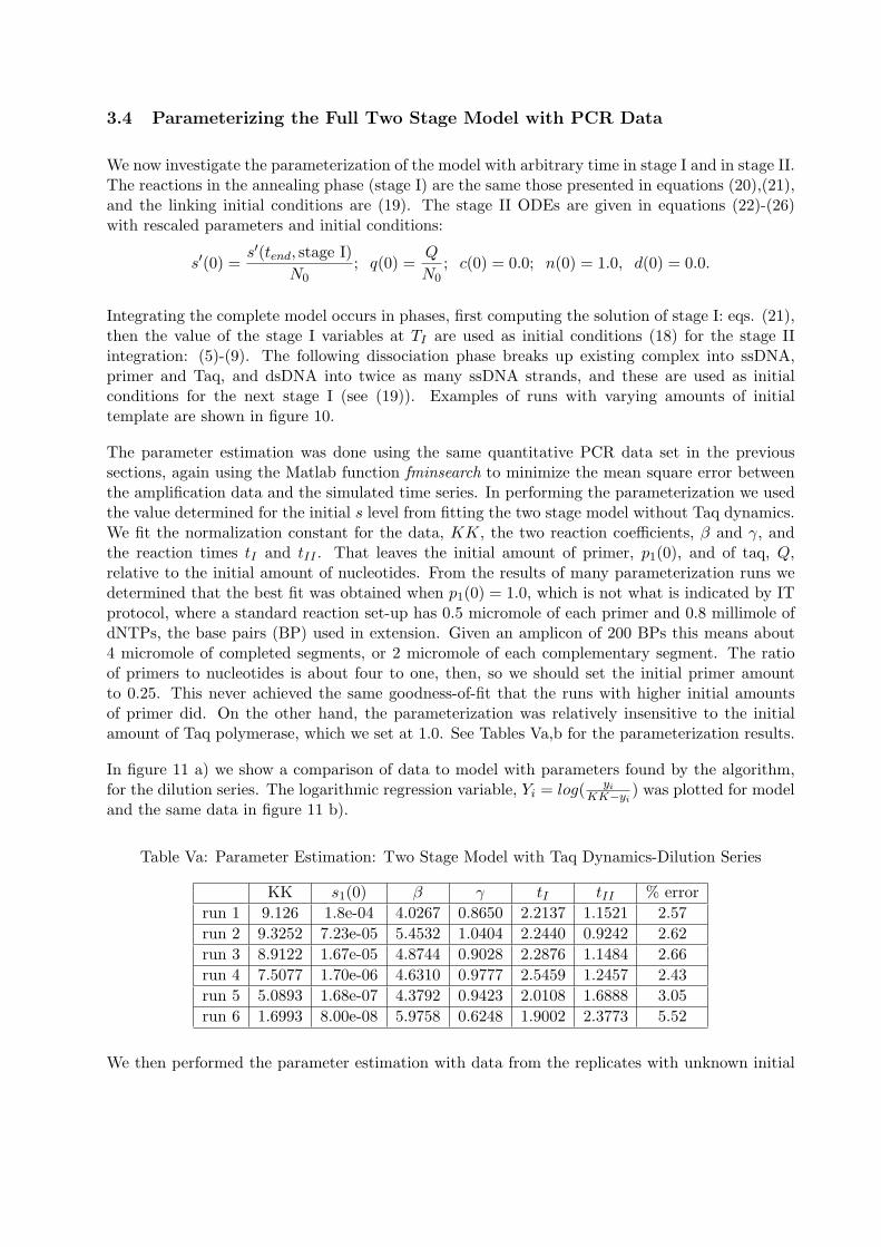
Table Va: Parameter Estimation: Two Stage Model with Taq Dynamics-Dilution Series
KK s1(0) β γ tI tII % errorrun 1 9.126 1.8e-04 4.0267 0.8650 2.2137 1.1521 2.57run 2 9.3252 7.23e-05 5.4532 1.0404 2.2440 0.9242 2.62run 3 8.9122 1.67e-05 4.8744 0.9028 2.2876 1.1484 2.66run 4 7.5077 1.70e-06 4.6310 0.9777 2.5459 1.2457 2.43run 5 5.0893 1.68e-07 4.3792 0.9423 2.0108 1.6888 3.05run 6 1.6993 8.00e-08 5.9758 0.6248 1.9002 2.3773 5.52
We then performed the parameter estimation with data from the replicates with unknown initial
0 10 20 30 40 500
0.2
0.4
0.6
0.8
1
cycle number i
s i
increasing s0
Figure 10: Integration of the coupled ODE model, with varying initial template amount, s0(0).
concentrations, the results are presented in Table Vb.
Table Vb: Parameter Estimation: Two Stage Model with Taq Dynamics-Unknown SamplesKK s1(0) β γ tI tII % error
sample 1a 10.13 8.02e-05 0.8133 1.5316 2.5651 1.8070 3.42sample 1b 10.49 7.87e-05 1.7851 0.7927 3.3509 1.6211 3.32sample 1c 10.42 7.67e-05 3.1262 2.2279 4.3212 0.6089 2.86sample 1d 10.73 7.57e-05 4.5382 1.3121 4.2464 0.7309 2.86sample 1e 10.82 7.42e-05 5.4529 1.3825 3.1713 0.6814 2.90sample 2a 7.18 1.51e-06 7.6983 1.2537 4.7358 0.7902 2.76sample 2b 7.54 1.40e-06 4.6407 0.7659 4.2093 1.3862 2.60sample 2c 7.60 1.40e-06 5.4337 0.9113 3.6034 1.1658 2.67sample 2d 7.78 1.39e-06 6.7849 0.8755 3.4071 1.1475 2.64sample 2e 7.50 1.50e-06 4.7158 0.7127 3.6256 1.4914 2.73
Comparing the fitted parameters for the different replicates in the unknown sample runs pointsout an obvious flaw with this parameterization. There is clearly more than one parameter setwith an equally good fit to the data, meaning hidden dependencies in the parameters that simplerescaling cannot uncover. Determining these dependencies through alternative rescalings andsingular perturbation analysis, and through other parameter estimation techniques is the subjectof ongoing research.
Turning to the problem of realistic initial primer concentration, we found that for values muchless than 1.0 the model did not capture the non-logistic behavior of the data. This can be seenin figure 11 b), where the curves have a concave down portion near the end of the run, indicatingthe slowing of growth of the amplicon. In figure 12 we illustrate this by graphing the logarith-

0 5 10 15 20 25 30 35 40 45−0.1
0
0.1
0.2
0.3
0.4
0.5
0.6
0.7
0.8
0.9
cycle number
fluor
esce
nce
leve
l
decreasing s0
0 5 10 15 20 25 30 35 40 45−16
−14
−12
−10
−8
−6
−4
−2
0
2
4
Yn
cycle number n
decreasing s0
Figure 11: Comparison of two stage model with Taq dynamics to data. a) amplification curves,b) logarithmic regression curves. The data is represented with dashed lines. See the text forparameter values.
0 10 20 30 40 50 60 70−10
−8
−6
−4
−2
0
2
4
6
8
cycle number i
Yi
decreasing P(0) P(0) = 1.0
P(0) = 0.5
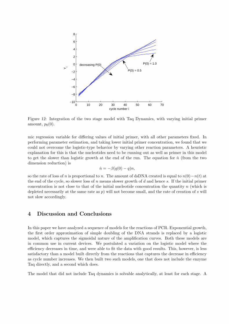
Figure 12: Integration of the two stage model with Taq Dynamics, with varying initial primeramount, p0(0).
mic regression variable for differing values of initial primer, with all other parameters fixed. Inperforming parameter estimation, and taking lower initial primer concentration, we found that wecould not overcome the logistic-type behavior by varying other reaction parameters. A heuristicexplanation for this is that the nucleotides need to be running out as well as primer in this modelto get the slower than logistic growth at the end of the run. The equation for n (from the twodimension reduction) is
n = −β(q(0)− q)n,
so the rate of loss of n is proportional to n. The amount of dsDNA created is equal to n(0)−n(t) atthe end of the cycle, so slower loss of n means slower growth of d and hence s. If the initial primerconcentration is not close to that of the initial nucleotide concentration the quantity n (which isdepleted necessarily at the same rate as p) will not become small, and the rate of creation of s willnot slow accordingly.
4 Discussion and Conclusions
In this paper we have analyzed a sequence of models for the reactions of PCR. Exponential growth,the first order approximation of simple doubling of the DNA strands is replaced by a logisticmodel, which captures the sigmoidal nature of the amplification curves. Both these models arein common use in current devices. We postulated a variation on the logistic model where theefficiency decreases in time, and were able to fit the data with good results. This, however, is lesssatisfactory than a model built directly from the reactions that captures the decrease in efficiencyas cycle number increases. We then built two such models, one that does not include the enzymeTaq directly, and a second which does.
The model that did not include Taq dynamics is solvable analytically, at least for each stage. A

map is created by linking the closed form solutions by their initial conditions. It was found thatthe data could be well estimated by reasonable parameter values if the initial amount of primerwas taken close to that of the initial amount of nucleotide. This is not the protocol followed inthe experiment, however, where for a 200 BP sequence the primer:nucleotide ratio is about 1:4. Itappears that the amount of nucleotides in the reaction must decrease significantly by the end of thereaction in order to obtain a decrease in overall reaction efficiency. For this to happen the initialconcentration of primer must about that of the nucleotide. From these observations we concludedthat the model without Taq dynamics did not capture the full behavior of the amplification curves.
The second model is built on reactions that include the formation of a complex of primed ssDNAand the Taq enzyme. The equations of stage I could still be solved analytically, but this was notpossible for stage II. Instead limiting cases of long integration time in stage I or stage II or bothwere considered, and by analyzing the amplification curves created by these maps we concludedthat none of the limiting cases, including variable annealing and long time extension, would createthe desired behavior at the end of the reaction. If the extension stage of the reaction was very fastcompared to the annealing phase, you might expect to capture the qualitative behavior with thislast case.
As none of the limiting cases created the qualitative end-of-reaction behavior we thought thedata demonstrate so clearly, we proceeded to parameterize the full equations for the two stagemodel with Taq dynamics. With a map created from solutions to these we were able to findparameters that captured the decreased efficiency at the end of the reaction, but only if initialprimer concentration was again roughly the same size as the initial concentration of nucleotides.The extension phase of the reaction would need to slow according to fit this aspect of the behavior.Also, multiple sets of parameters were found to fit the same amplification run, indicating hiddendependencies in the parameters that simple rescaling does not uncover.
While we were not able to completely explain the reduced efficiency seen in the data with our suiteof models, we were able to determine what portions of the model were important in capturing itsnon-logistic character. Competing reactions at higher cycle numbers most certainly will have aneffect on the efficiency, especially with the lower initial copy number runs. Future work will includeanalyzing these dependencies both numerically and analytically, and using the two stage model toseek reaction protocols that minimize time to almost complete creation of amplicon, and maximizeyield for a fixed total cycle time.
Acknowledgements
We would like to thank Dr. David Eyre, Idaho Technology, for suggesting the problem and forproviding us with IT data and much consultation. This work was partially supported by a UtahState University Community/University Initiative grant, a USU Center for Integrated Biosystemsseed grant, and one undergraduate (John Goldes) was supported by NSF-EPSCoR funds at theUniversity of Montana-Missoula.

Appendix: Linear stability analysis for stage II with Taq Dynamics
This stability analysis uses the two dimensional system that takes advantage of the conservedquantities, s′ + c + d = s′(0), q + c = q(0), and n + d = 1.
q = −γ(s′(0)− q(0)− 1 + q + n)q + q(0)− q + β(q(0)− q)n
n = −β(q(0)− q)n.
The fixed points
Solving q = 0 and n = 0 simultaneously gives three fixed points.
f.p.1 = (q = q(0), n = 1− s′(0))
f.p.2 = (q =12γ
(γ(q(0) + 1− s′(0))− 1 +√
(−γ(q(0) + 1− s′(0)) + 1)2 + 4γq(0)),
n = 0)
The third fixed point has
q =12γ
(γ(q(0) + 1− s′(0))− 1−√
(−γ(q(0) + 1− s′(0)) + 1)2 + 4γq(0)),
which is always negative. Proof:
q is a root of the polynomial γq2+(−γ(q(0)+1−s′(0))+1)q−q(0). Let b = −γ(q(0)+1−s′(0))+1.Then √
b2 + 4γq(0) > b,
therefore,−b−
√b2 + 4γq(0) < 0.
Since f.p.3 is not of physical importance, we will only analyze the stability of f.p. 1 and f.p. 2.
Stability of f.p.1
The Jacobian for the reduced system is[ −γ q − γ (s′(0)− q(0)− 1 + q + n)− 1− β n −γ q + β (q(0)− q)
β n −β (q(0)− q)
]
Let s′(0), q(0) > 0, c(0) = 0, n(0) = 1, and d(0) = 0. Also let γ, β > 0. For f.p. 1, the Jacobianbecomes [ −γ q(0)− 1− β (1− s′(0)) −γ q(0)
β (1− s′(0)) 0
]

The eigenvalues are,
1/2(−γq(0)− 1− β(1− s′(0))±√
(γq(0) + 1 + β(1− s′(0)))2 − 4γq(0)β(1− s′(0))).
The location of the first fixed point and the sign of the nonzero eigenvalues depend on the rela-tionship between n(0) = 1 and s′(0).
Case1: 1 > s′(0) ⇒ 1 − s′(0) > 0 Both coordinates of the first fixed point are non-negative. Theeigenvalues are real and negative. They are real because the discriminant is greater than zero.Proof:
(γq(0) + 1 + β(1− s′(0)))2 − 4γq(0)β(1− s′(0))
= γ2q(0)2 + 2γq(0) + 2γq(0)β(1− s′(0)) + 2β(1− s′(0)) + 1 + β2(1− s′(0))2 − 4γq(0)β(1− s′(0))
= γ2q(0)2 − 2γq(0)β(1− s′(0)) + β2(1− s′(0))2 + 2γq(0) + 2β(1− s′(0)) + 1
= (γq(0)− β(1− s′(0)))2 + 2γq(0) + 2β(1− s′(0)) + 1 > 0.
They are both negative. Proof:
Letb = γq(0) + 1 + β(1− s′(0)). Then b2 > 4γq(0)β(1− s′(0)) as shown above.√
b2 − 4γq(0)β(1− s′(0)) < b,
therefore,−b +
√b2 − 4γq(0)β(1− s′(0))
2and
−b−√
b2 − 4γq(0)β(1− s′(0))2
are both < 0.
Case 2: n(0) = 1 = s′(0) ⇒ 1 − s′(0) = 0. The first fixed point becomes (q(0), 0) which still isnonnegative. The eigenvalues become:
12(−γq(0)− 1 +
√(γq(0) + 1)2) =
12(−γq(0)− 1 + γq(0) + 1) = 0
and12(−γq(0)− 1−
√(γq(0) + 1)2) =
12(−2γq(0)− 2) = −γq(0)− 1.
For this case, there is only one nonzero eigenvalue, −γq(0)− 1. −γq(0)− 1 < 0, so this eigenvalueis negative.
Case3: n(0) = 1 < s′(0) ⇒ 1− s′(0) < 0. The coordinate, n = 1− s′(0), of the first fixed point isnow negative. The eigenvalues,
1/2(−γq(0)− 1− β(1− s′(0))±√
(γq(0) + 1 + β(1− s′(0)))2 − 4γq(0)β(1− s′(0))),
are real. Proof:
Let α > 0 and let 1− s′(0) = −α. Let
b = γq(0) + 1 + β(−α) = γq(0) + 1− βα.

b2 − 4γq(0)β(−α) = b2 + 4γq(0)βα,
thereforeb2 + 4γq(0)βα > 0.
One of the nonzero eigenvalues is positive and the other is negative. Proof:
b2 + 4γq(0)βα > 0, so√
b2 + 4γq(0)βα > b. Then
−b +√
b2 + 4γq(0)βα
2> 0
and−b−
√b2 + 4γq(0)βα
2< 0.
Stability of f.p.2
For f.p.2, the Jacobian becomes[ −γ q − γ (s′(0)− q(0)− 1 + q)− 1 −γ q + β (q(0)− q)
0 −β (q(0)− q)
]
where q = 12γ (γ(q(0)+1−s′(0))−1+
√(−γ(q(0) + 1− s′(0)) + 1)2 + 4γq(0)). The eigenvalues are
β
2γ(−γq(0) + γ(1− s′(0))− 1 +
√(γq(0)− γ(1− s′(0)) + 1)2 + 4γ2q(0)(1− s′(0)),
−√
(γq(0)− γ(1− s′(0)) + 1)2 + 4γ2q(0)(1− s′(0)).
Case1: 1− s′(0) > 0 For this case q is positive. Proof:
Let b = −γ(q(0) + 1− s′(0)) + 1. b2 + 4γq(0) > 0, so√
b2 + 4γq(0) > b. Therefore,
−b +√
b2 + 4γq(0))2γ
> 0.
The eigenvalues are both real. Proof:
(γq(0)− γ(1− s′(0)) + 1)2 > 0.
Also, for 1 − s′(0) > 0, 4γ2q(0)(1 − s′(0)) > 0. Therefore, the discriminant is positive. Theeigenvalue
−√
(γq(0)− γ(1− s′(0)) + 1)2 + 4γ2q(0)(1− s′(0))
is clearly negative. The other eigenvalue is positive for this case. Proof:
Let b = γq(0)− γ(1− s′(0)) + 1.
b <√
b2 + 4γ2q(0)(1− s′(0))

therefore,−b +
√b2 + 4γ2q(0)(1− s′(0)) > 0
Case 2: 1− s′(0) = 0. For this case, f.p.1 = f.p.2. Proof:
q =12γ
(γq(0)− 1 +√
(−γq(0) + 1)2 + 4γq(0))
=12γ
(γq(0)− 1 +√−γ2q(0)2 − 2γq(0) + 1 + 4γq(0))
=12γ
(γq(0)− 1 +√−γ2q(0)2 + 2γq(0) + 1
=12γ
(γq(0)− 1 +√
(γq(0) + 1)2
=12γ
(γq(0)− 1 + γq(0) + 1) =12γ
(2γq(0))
= q(0).
f.p.2 becomes q = (q(0), n = 0) which equals f.p.1.
Case 3: 1 − s′(0) < 0. The eigenvalues remain real for this case, but the one that was positive inCase 1 becomes negative. Proof:
Let −α = 1− s′(0), α > 0, and let b = γq(0) + γα + 1. Then
b >√
b2 − 4γ2q(0)α
therefore,−b +
√b2 − 4γ2q(0)α < 0
Conclusion
For Case 1, f.p.1 is a sink, but becomes a saddle as s’(0) becomes larger than n(0)(for Case 3). Theopposite occurs for f.p.2. It starts out as a saddle (for Case 1) and becomes a sink (for Case 3).This indicates a transcritical bifurcation when the initial amount of nucleotides equals the initialamount of primed single-strand DNA.
References
[1] Morrison T., J. Weis and C. Wittwer (1998) Quantification of low copy transcripts by contin-uous SYBR Green I monitoring during amplification. BioTechniques 24 954–962.
[2] Schnell S., and C. Mendoza (1997) Ensymological considerations for a theoretical description ofthe quantitative competitive polymerase chain reaction (QC-PCR). J. Theor. Biol. 184 433–440.
[3] Stolovitzky, G. and G. Cecchi (1996) Efficiency of DNA replication in the polymerase chainreaction. Proc. Natl. Acad. Sci. USA. 93 12947–12952.

[4] Sun, F. (1995) The polymerase chain reaction and branching processes. J. Comp. Bio. 2 no. 1,63–86.
[5] Sun, F., D. Galas and M. Waterman (1996) A mathematical analysis of in vitro molecularselection-amplification. J. Mol. Biol. 258 650–660.
[6] Weiss, G and A. von Haeseler (1995) Modeling the polymerase chain reaction. J. Comput. Biol.2 49–61.
[7] Weiss, G. and A. von Haeseler (1997) A coalescent approach to the polymerase chain reaction.Nucleic Acids Res. 25 3082–3087.
[8] Whitney, S., A. Sudhir, R. M. Nelson and H. Viljoen (2004) Principles of rapid polymerasechain reactions: mathematical modeling and experimental verification. Comp. Bio. and Chem.28 195–209.
[9] Wittwer, C., G. Reed, and K. Ririe (1994) Rapid cycle DNA amplification, in K Mullis, F.Ferre, and R Gibbs (Eds.), The Polymerase Chain Reaction. Springer-Verlag, Deerfield Beach,FL, 174–181.
[10] Wittwer C., M. Herrmann, A. Moss and R. Rasmussen (1997) Continuous fluorescence mon-itoring of rapid cycle DNA amplification. BioTechniques 22 130–138.
[11] Wittwer C., K. Ririe and R. Rasmussen (1998). Fluorescence monitoring of rapid cycle PCRfor quantification. In: Ferre F, ed. Gene Quantification. Birkhauser, Boston MA 129–144.
[12] Velikanov, M. and R. Kapral (1999) Polymerase chain reaction: A markov process approach.J. theor. Biol. 201 239–249.
[13] Viljoen, S., M. Griep, M. Nelson and H. Viljoen (2005) A macroscopic kinetic model for DNApolymerase elongation and high-fidelity nucleotide selection. Comp. Bio. and Chem. 29 101–110.