A Tutorial on theComputation of Bayes Factors

Insper Working PaperWPE: 341/2014

Hedibert Freitas Lopes

A Tutorial on the1

Computation of Bayes Factors2

Hedibert Freitas Lopes3

INSPER Institute of Education and Research4

Rua Quata 300, Vila Olımpia5

Sao Paulo/SP - Brazil - 04546-0426

E-mail:hedibertFL@insper.edu.br7

Abstract8

In this review paper we revisit several of the existing schemes that approx-9

imate predictive densities and, consequently, Bayes factors. We also present10

the reversible jump MCMC scheme, which can be thought of as an MCMC11

scheme over the space of models. These approaches are applied to select the12

number of common factors in the basic normal linear factor model, which is a13

high profile example within the psychometrics community.14

1 Introduction15

Bayesian model comparison is commonly (but not exclusively) performed by com-16

puting posterior model probabilities. Suppose that the competing models can be17

enumerated and are represented by the set M = M1,M2, . . .. Under model Mj18

with corresponding parameter vector θj, the posterior distribution of θj is obtained19

in the usual manner20

p(θj|Mj, y) =p(y|θj,Mj)p(θj|Mj)

p(y|Mj), (1)

where p(y|θj,Mj) and p(θj|Mj) respectively represent the likelihood and the prior21

distribution of θj under model Mj. Predictive densities (aka normalizing constants22

or marginal likelihoods)23

p(y|Mj) =∫p(y|θj,Mj)p(θj|Mj)dθj, (2)

1

play an important role in Bayesian model selection and comparison. The posterior24

odds of model Mj relative to model Mk is defined as Pr(Mj|y)/Pr(Mk|y), which25

is the product of the prior odds Pr(Mj)/Pr(Mk) of model Mj relative to model26

Mk by the Bayes factor,27

Bjk =p(y|Mj)

p(y|Mk). (3)

The Bayes factor can be viewed as the weighted likelihood ratio ofMj toMk. Hence,28

the posterior model probability for model j is29

Pr(Mj|y) =

∞∑k=1

BkjPr(Mk)

Pr(Mj)

−1, (4)

which depends on all prior odds ratios and all Bayes factors involving model j.30

When the prior model probabilities are uniformly distributed, the posterior model31

probabilities equal the Bayes factor. Jeffreys (1961) recommends the use of the32

following rule of thumb to decide between models j and k: when Bjk is above 100,33

between 10 and 100 and between 3 and 10, there is decisive, strong or substantial34

evidence against k, respectively.35

Markov Chain Monte Carlo methods freed the Bayesian community by accurately36

approximating posterior distributions, p(θj|Mj, y), for virtually all sorts of model37

structures. However, one can argue that the hardest computational task for an38

applied Bayesian is the computation of the normalizing constant p(y|Mj), which39

involves a multidimensional integral in θj.40

In this review paper we revisit several of the existing schemes that approximate41

predictive densities, p(y|M), and, consequently, Bayes factors. We also present the42

reversible jump MCMC scheme, which can be thought of as an MCMC scheme over43

the space of models. These two approaches are presented in Sections 3 and 4, respec-44

tively, following Section 2 where the basic normal linear factor model is introduced as45

a motivational high profile example within the psychometrics community. The fac-46

tor model appears again in Section 5 through a computationally intensive simulated47

exercise. We conclude in Section 6.48

2

2 Factor analysis49

We will use the basic linear Gaussian factor model framework as an illustration of50

the computation of Bayes factors. In the factor analysis case, competing models have51

distinct number of common factors. The origin of factor analysis can be tracked back52

to Spearman’s (1904) seminal paper on general intelligence. At the time, psychol-53

ogists were trying to define intelligence by a single, all-encompassing unobservable54

entity, the g factor. Spearman studied the influence of the g factor on examinees test55

scores on several domains: pitch, light, weight, classics, french, english and mathe-56

matics. At the end of the day, the g factor would provide a mechanism to detect57

common correlations among such imperfect measurements.58

Spearman’s (1904) one-factor model based on p test domains (measurements) and59

n examinees (individuals) can be written as60

yij = µj + βjgi + εij, (5)

for i = 1, . . . , n, j = 1, . . . , p, where yij is the score of examinee i on test domain j,61

µj is the mean of test domain j, gi is the value of the intelligence factor for person i,62

βj is the loading of test domain j onto the intelligence factor g and εij is the random63

error term for person i and test domain j. For subsequent developments, mainly64

in psychology studies, see Burt (1940), Holzinger and Harman (1941) and Thomson65

(1953), amongst others, where the factors had a priori known structure.66

The extension to multiple factors as well as its formal statistical framework come67

many decades later. Multiple factor analysis were first introduced by Thurstone68

(1935,1947) and Lawley (1940,1953), along with estimation via centroid method and69

maximum likelihood, respectively. Hotelling (1955) proposed a more robust method70

of estimation, the method of principal components, while Anderson and Rubin (1956)71

formalized and elevated factor analysis to the realm of statistically and probabilis-72

tically sound modeling schemes. Maximum likelihood estimation became practical73

in the late 1960s through the work of Joreskog(1967,1969). A further improvement74

was achieved in the early 1980s through the EM algorithms of Rubin and Thayer75

(1982,1983); see also Bentler and Tanaka (1983). In the late 1980s, Anderson and76

Amemiya (1988) and Amemiya and Anderson (1990), studied the asymptotic be-77

havior of estimation and hypothesis testing for a large class of factor analysis under78

3

general conditions, while Akaike (1987) proposed an information criterion to select-79

ing the proper number of common factors. To celebrate the centennial of Spearman80

(1904), The L. L. Thurstone Psychometric Laboratory, University of North Carolina81

at Chapel Hill, hosted in May 2004 a workshop entitled Factor Analysis at 100: His-82

torical Developments and Future Directions. The papers presented at the meeting83

appeared in Cudeck and MacCallum (2007).84

Bayesian normal linear factor analysis. Let yi = (yi1, . . . , yip)′, for i = 1, . . . , n,85

be a p-dimensional vector with the measurements on p related variables (Spearman’s86

tests, attributes, macroeconomic or financial time-series, census sectors, monitoring87

stations, to name a few examples). The basic normal linear factor model assumes that88

ys are independent and identically distributed N(0,Ω), ie. a zero-mean multivariate89

normal with a p × p non-singular variance matrix Ω. Loosely speaking, a factor90

model usually rewrites Ω, which depends of q = p(p + 1)/2 variance and covariance91

components, as a function of d parameters, where d is potentially many orders of92

magnitude smaller than q.93

More specifically, for any positive integer k ≤ p, a standard normal linear k-factor94

model for yi is written as95

yi|fi, β,Σ, k ∼ N(βfi,Σ) (6)

fi|H, k ∼ N(0, H) (7)

where fi is the k-dimensional vector of common factors, β is the p × k matrix of96

factor loadings, Σ = diag(σ21, · · · , σ2

p) is the covariance of the specific factors and H =97

diag(h1, . . . , hk) is the covariance matrix of the common factors. The uniquenesses98

σ2i s, also known as idiosyncratic or specific variances, measure the residual variability99

in each of the data variables once that contributed by the factors is accounted for.100

Conditionally on the common factors, fk, the measurements in yi are independent.101

In other words, the common factors explain all the dependence structure among102

the p variables and, based on equations (6) and (7), the unconditional, constrained103

covariance matrix of yi (a function of k) becomes104

Ω = βHβ′ + Σ. (8)

4

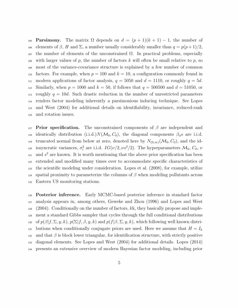
Parsimony. The matrix Ω depends on d = (p + 1)(k + 1) − 1, the number of105

elements of β, H and Σ, a number usually considerably smaller than q = p(p+ 1)/2,106

the number of elements of the unconstrained Ω. In practical problems, especially107

with larger values of p, the number of factors k will often be small relative to p, so108

most of the variance-covariance structure is explained by a few number of common109

factors. For example, when p = 100 and k = 10, a configuration commonly found in110

modern applications of factor analysis, q = 5050 and d = 1110, or roughly q = 5d.111

Similarly, when p = 1000 and k = 50, if follows that q = 500500 and d = 51050, or112

roughly q = 10d. Such drastic reduction in the number of unrestricted parameters113

renders factor modeling inherently a parsimonious inducing technique. See Lopes114

and West (2004) for additional details on identifiability, invariance, reduced-rank115

and rotation issues.116

Prior specification. The unconstrained components of β are independent and117

identically distribution (i.i.d.)N(M0, C0), the diagonal components βiis are i.i.d.118

truncated normal from below at zero, denoted here by N(0,∞)(M0, C0), and the id-119

iosyncratic variances, σ2i are i.i.d. IG(ν/2, νs2/2). The hyperparameters M0, C0, ν120

and s2 are known. It is worth mentioning that the above prior specification has been121

extended and modified many times over to accommodate specific characteristics of122

the scientific modeling under consideration. Lopes et al. (2008), for example, utilize123

spatial proximity to parameterize the columns of β when modeling pollutants across124

Eastern US monitoring stations.125

Posterior inference. Early MCMC-based posterior inference in standard factor126

analysis appears in, among others, Geweke and Zhou (1996) and Lopes and West127

(2004). Conditionally on the number of factors, kk, they basically propose and imple-128

ment a standard Gibbs sampler that cycles through the full conditional distributions129

of p(β|f,Σ, y, k), p(Σ|f, β, y, k) and p(f |β,Σ, y, k), which following well known distri-130

butions when conditionally conjugate priors are used. Here we assume that H = Ik131

and that β is block lower triangular, for identification structure, with strictly positive132

diagonal elements. See Lopes and West (2004) for additional details. Lopes (2014)133

presents an extensive overview of modern Bayesian factor modeling, including prior134

5

and posterior robustness, mixture of factor analyzers, factor analysis in time series135

and macro-econometric modeling and sparse factor structures in micro-econometrics136

and genomics. He also lists some of the recent contributions to the literature on137

non-Bayesian (large dimensional and/or dynamic) factor analysis.138

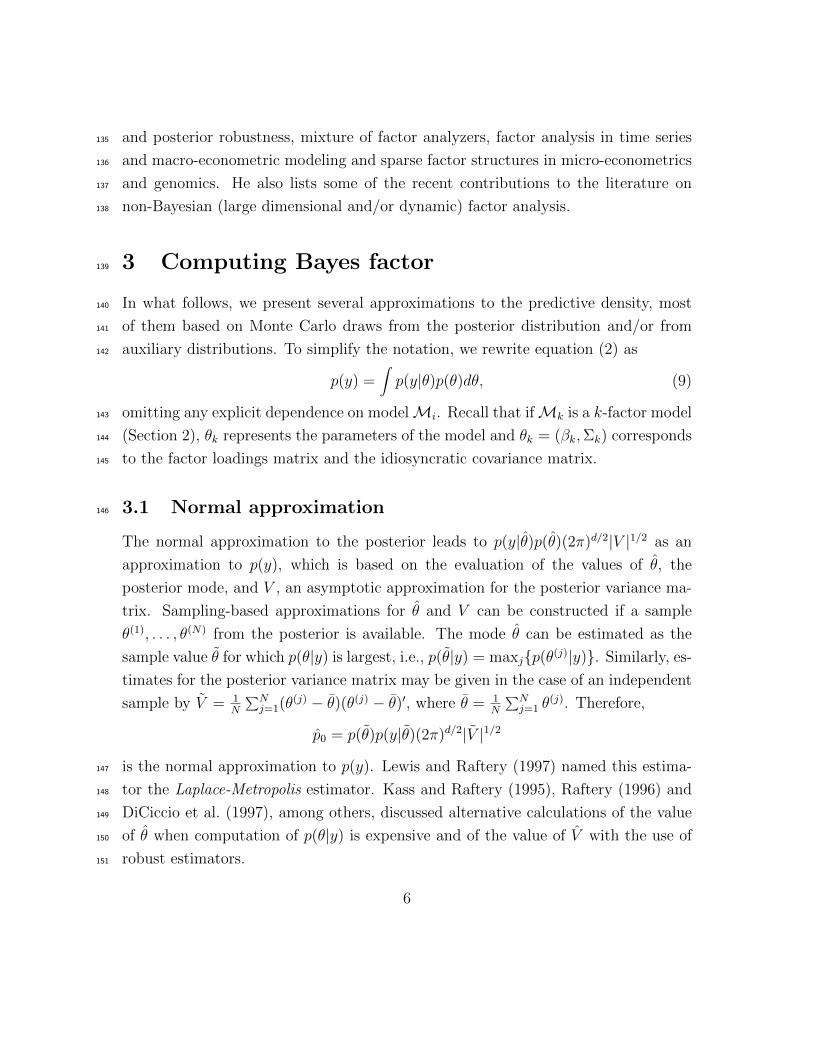
3 Computing Bayes factor139

In what follows, we present several approximations to the predictive density, most140

of them based on Monte Carlo draws from the posterior distribution and/or from141

auxiliary distributions. To simplify the notation, we rewrite equation (2) as142

p(y) =∫p(y|θ)p(θ)dθ, (9)

omitting any explicit dependence on modelMi. Recall that ifMk is a k-factor model143

(Section 2), θk represents the parameters of the model and θk = (βk,Σk) corresponds144

to the factor loadings matrix and the idiosyncratic covariance matrix.145

3.1 Normal approximation146

The normal approximation to the posterior leads to p(y|θ)p(θ)(2π)d/2|V |1/2 as an

approximation to p(y), which is based on the evaluation of the values of θ, the

posterior mode, and V , an asymptotic approximation for the posterior variance ma-

trix. Sampling-based approximations for θ and V can be constructed if a sample

θ(1), . . . , θ(N) from the posterior is available. The mode θ can be estimated as the

sample value θ for which p(θ|y) is largest, i.e., p(θ|y) = maxjp(θ(j)|y). Similarly, es-

timates for the posterior variance matrix may be given in the case of an independent

sample by V = 1N

∑Nj=1(θ

(j) − θ)(θ(j) − θ)′, where θ = 1N

∑Nj=1 θ

(j). Therefore,

p0 = p(θ)p(y|θ)(2π)d/2|V |1/2

is the normal approximation to p(y). Lewis and Raftery (1997) named this estima-147

tor the Laplace-Metropolis estimator. Kass and Raftery (1995), Raftery (1996) and148

DiCiccio et al. (1997), among others, discussed alternative calculations of the value149

of θ when computation of p(θ|y) is expensive and of the value of V with the use of150

robust estimators.151

6

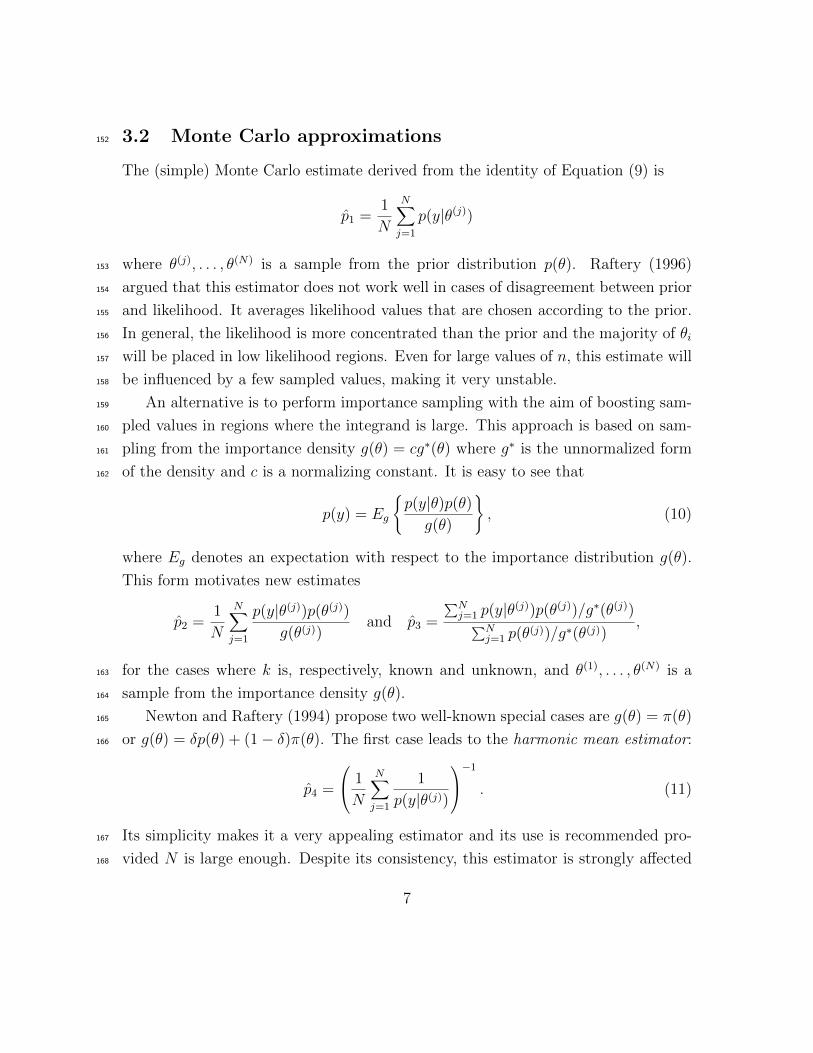
3.2 Monte Carlo approximations152

The (simple) Monte Carlo estimate derived from the identity of Equation (9) is

p1 =1

N

N∑j=1

p(y|θ(j))

where θ(j), . . . , θ(N) is a sample from the prior distribution p(θ). Raftery (1996)153

argued that this estimator does not work well in cases of disagreement between prior154

and likelihood. It averages likelihood values that are chosen according to the prior.155

In general, the likelihood is more concentrated than the prior and the majority of θi156

will be placed in low likelihood regions. Even for large values of n, this estimate will157

be influenced by a few sampled values, making it very unstable.158

An alternative is to perform importance sampling with the aim of boosting sam-159

pled values in regions where the integrand is large. This approach is based on sam-160

pling from the importance density g(θ) = cg∗(θ) where g∗ is the unnormalized form161

of the density and c is a normalizing constant. It is easy to see that162

p(y) = Eg

p(y|θ)p(θ)g(θ)

, (10)

where Eg denotes an expectation with respect to the importance distribution g(θ).

This form motivates new estimates

p2 =1

N

N∑j=1

p(y|θ(j))p(θ(j))g(θ(j))

and p3 =

∑Nj=1 p(y|θ(j))p(θ(j))/g∗(θ(j))∑N

j=1 p(θ(j))/g∗(θ(j))

,

for the cases where k is, respectively, known and unknown, and θ(1), . . . , θ(N) is a163

sample from the importance density g(θ).164

Newton and Raftery (1994) propose two well-known special cases are g(θ) = π(θ)165

or g(θ) = δp(θ) + (1− δ)π(θ). The first case leads to the harmonic mean estimator:166

p4 =

1

N

N∑j=1

1

p(y|θ(j))

−1 . (11)

Its simplicity makes it a very appealing estimator and its use is recommended pro-167

vided N is large enough. Despite its consistency, this estimator is strongly affected168

7

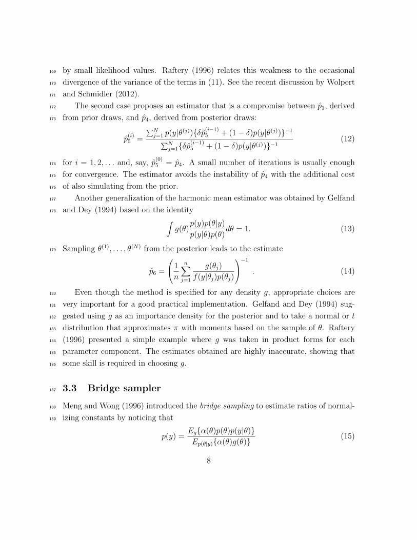
by small likelihood values. Raftery (1996) relates this weakness to the occasional169

divergence of the variance of the terms in (11). See the recent discussion by Wolpert170

and Schmidler (2012).171

The second case proposes an estimator that is a compromise between p1, derived172

from prior draws, and p4, derived from posterior draws:173

p(i)5 =

∑Nj=1 p(y|θ(j))δp

(i−1)5 + (1− δ)p(y|θ(j))−1∑N

j=1δp(i−1)5 + (1− δ)p(y|θ(j))−1

(12)

for i = 1, 2, . . . and, say, p(0)5 = p4. A small number of iterations is usually enough174

for convergence. The estimator avoids the instability of p4 with the additional cost175

of also simulating from the prior.176

Another generalization of the harmonic mean estimator was obtained by Gelfand177

and Dey (1994) based on the identity178 ∫g(θ)

p(y)p(θ|y)

p(y|θ)p(θ)dθ = 1. (13)

Sampling θ(1), . . . , θ(N) from the posterior leads to the estimate179

p6 =

1

n

n∑j=1

g(θj)

f(y|θj)p(θj)

−1 . (14)

Even though the method is specified for any density g, appropriate choices are180

very important for a good practical implementation. Gelfand and Dey (1994) sug-181

gested using g as an importance density for the posterior and to take a normal or t182

distribution that approximates π with moments based on the sample of θ. Raftery183

(1996) presented a simple example where g was taken in product forms for each184

parameter component. The estimates obtained are highly inaccurate, showing that185

some skill is required in choosing g.186

3.3 Bridge sampler187

Meng and Wong (1996) introduced the bridge sampling to estimate ratios of normal-188

izing constants by noticing that189

p(y) =Egα(θ)p(θ)p(y|θ)Ep(θ|y)α(θ)g(θ)

(15)

8

for any arbitrary bridge function α(θ) with support encompassing both supports

of the posterior density π and the proposal density g. If α(θ) = 1/g(θ) then

the bridge estimator reduces to the simple Monte Carlo estimator p1. Similarly,

if α(θ) = p(θ)p(y|θ)g(θ)−1 then the bridge estimator is a variation of the har-

monic mean estimator. They showed that the optimal mean square error α func-

tion is α(θ) = g(θ) + (M/N)π(θ)−1, which depends on f(y) itself. By letting

ω(j) = (θ(i))p(θ(i))/g(θ(i)), for j = 1, . . . , N and ω(i) = p(y|θ(i))p(θ(i))/g(θ(i)), for

j = 1, . . . ,M , they devised the iterative scheme to estimate p(y):

p(i)7 =

1M

∑Mj=1 ω

(j)[s1ω(j) + s2p

(i−1)7 ]−1

1N

∑Nj=1[s1ω

(j) + s2p(i−1)7 ]−1

,

for i = 1, 2, . . ., s1 = N/(M + N), s2 = M/(M + N) and, say, p(0)7 = p4. A small190

number of iterations is usually enough for convergence. See also Meng and Schilling191

(1996), Gelman and Meng (1997) and Meng and Schilling (2002). Gelman and Meng192

(1998) generalized the bridge sampling by replacing one (possibly long) bridge by193

infinitely many shorter bridges or, as they call it, a path.194

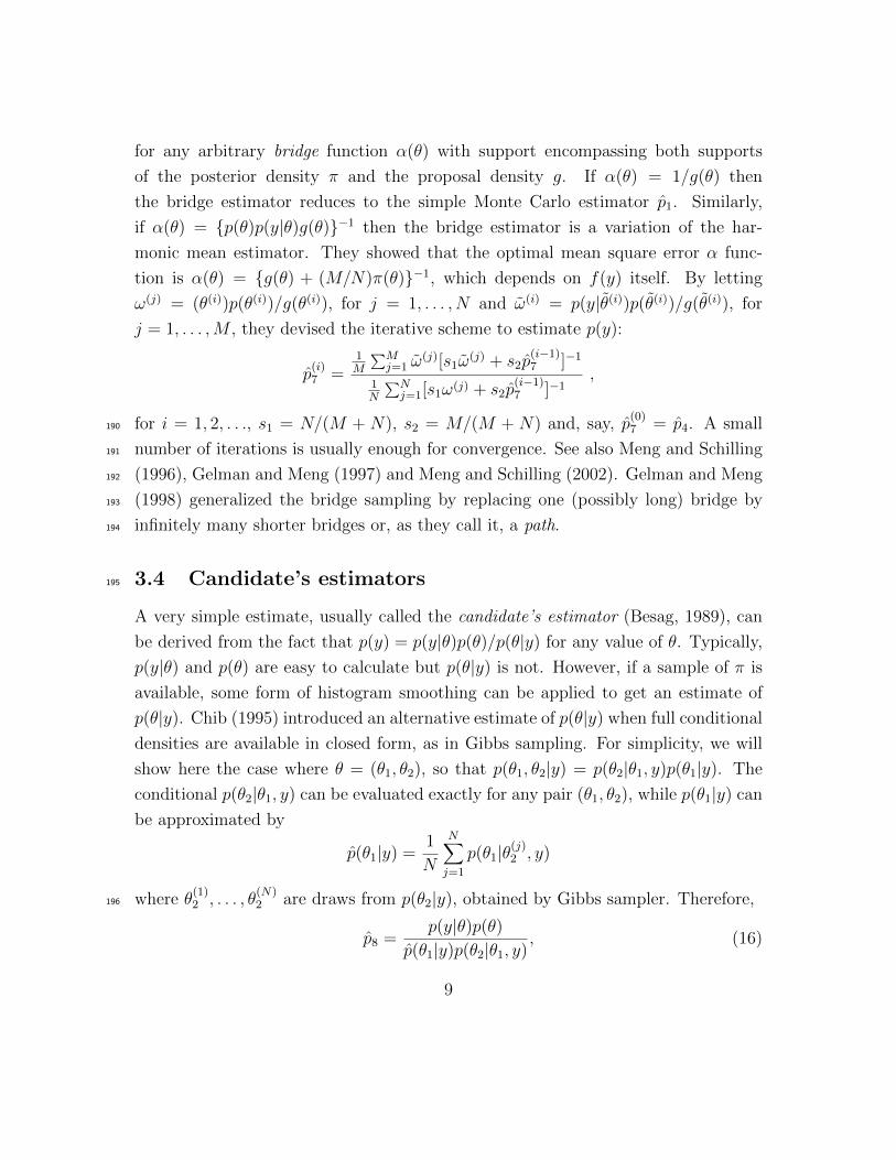
3.4 Candidate’s estimators195

A very simple estimate, usually called the candidate’s estimator (Besag, 1989), can

be derived from the fact that p(y) = p(y|θ)p(θ)/p(θ|y) for any value of θ. Typically,

p(y|θ) and p(θ) are easy to calculate but p(θ|y) is not. However, if a sample of π is

available, some form of histogram smoothing can be applied to get an estimate of

p(θ|y). Chib (1995) introduced an alternative estimate of p(θ|y) when full conditional

densities are available in closed form, as in Gibbs sampling. For simplicity, we will

show here the case where θ = (θ1, θ2), so that p(θ1, θ2|y) = p(θ2|θ1, y)p(θ1|y). The

conditional p(θ2|θ1, y) can be evaluated exactly for any pair (θ1, θ2), while p(θ1|y) can

be approximated by

p(θ1|y) =1

N

N∑j=1

p(θ1|θ(j)2 , y)

where θ(1)2 , . . . , θ

(N)2 are draws from p(θ2|y), obtained by Gibbs sampler. Therefore,196

p8 =p(y|θ)p(θ)

p(θ1|y)p(θ2|θ1, y), (16)

9

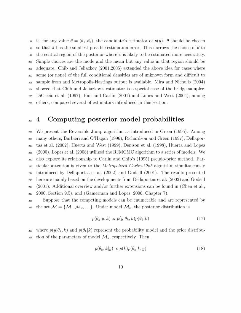
is, for any value θ = (θ1, θ2), the candidate’s estimator of p(y). θ should be chosen197

so that π has the smallest possible estimation error. This narrows the choice of θ to198

the central region of the posterior where π is likely to be estimated more accurately.199

Simple choices are the mode and the mean but any value in that region should be200

adequate. Chib and Jeliazkov (2001,2005) extended the above idea for cases where201

some (or none) of the full conditional densities are of unknown form and difficult to202

sample from and Metropolis-Hastings output is available. Mira and Nicholls (2004)203

showed that Chib and Jeliazkov’s estimator is a special case of the bridge sampler.204

DiCiccio et al. (1997), Han and Carlin (2001) and Lopes and West (2004), among205

others, compared several of estimators introduced in this section.206

4 Computing posterior model probabilities207

We present the Reversible Jump algorithm as introduced in Green (1995). Among208

many others, Barbieri and O’Hagan (1996), Richardson and Green (1997), Dellapor-209

tas et al. (2002), Huerta and West (1999), Denison et al. (1998), Huerta and Lopes210

(2000), Lopes et al. (2008) utilized the RJMCMC algorithm to a series of models. We211

also explore its relationship to Carlin and Chib’s (1995) pseudo-prior method. Par-212

ticular attention is given to the Metropolized Carlin-Chib algorithm simultaneously213

introduced by Dellaportas et al. (2002) and Godsill (2001). The results presented214

here are mainly based on the developments from Dellaportas et al. (2002) and Godsill215

(2001). Additional overview and/or further extensions can be found in (Chen et al.,216

2000, Section 9.5), and (Gamerman and Lopes, 2006, Chapter 7).217

Suppose that the competing models can be enumerable and are represented by218

the set M = M1,M2, . . .. Under model Mk, the posterior distribution is219

p(θk|y, k) ∝ p(y|θk, k)p(θk|k) (17)

where p(y|θk, k) and p(θk|k) represent the probability model and the prior distribu-220

tion of the parameters of model Mk, respectively. Then,221

p(θk, k|y) ∝ p(k)p(θk|k, y) (18)

10

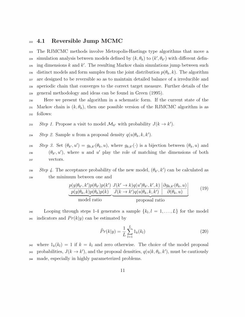
4.1 Reversible Jump MCMC222

The RJMCMC methods involve Metropolis-Hastings type algorithms that move a223

simulation analysis between models defined by (k, θk) to (k′, θk′) with different defin-224

ing dimensions k and k′. The resulting Markov chain simulations jump between such225

distinct models and form samples from the joint distribution p(θk, k). The algorithm226

are designed to be reversible so as to maintain detailed balance of a irreducible and227

aperiodic chain that converges to the correct target measure. Further details of the228

general methodology and ideas can be found in Green (1995).229

Here we present the algorithm in a schematic form. If the current state of the230

Markov chain is (k, θk), then one possible version of the RJMCMC algorithm is as231

follows:232

Step 1. Propose a visit to model Mk′ with probability J(k → k′).233

Step 2. Sample u from a proposal density q(u|θk, k, k′).234

Step 3. Set (θk′ , u′) = gk,k′(θk, u), where gk,k′(·) is a bijection between (θk, u) and235

(θk′ , u′), where u and u′ play the role of matching the dimensions of both236

vectors.237

Step 4. The acceptance probability of the new model, (θk′ , k′) can be calculated as238

the minimum between one and239

p(y|θk′ , k′)p(θk′)p(k′)p(y|θk, k)p(θk)p(k)︸ ︷︷ ︸

model ratio

J(k′ → k)q(u′|θk′ , k′, k)

J(k → k′)q(u|θk, k, k′)

∣∣∣∣∣∂gk,k′(θk, u)

∂(θk, u)

∣∣∣∣∣︸ ︷︷ ︸proposal ratio

(19)

Looping through steps 1-4 generates a sample kl, l = 1, . . . , L for the model240

indicators and Pr(k|y) can be estimated by241

P r(k|y) =1

L

L∑l=1

1k(kl) (20)

where 1k(kl) = 1 if k = kl and zero otherwise. The choice of the model proposal242

probabilities, J(k → k′), and the proposal densities, q(u|k, θk, k′), must be cautiously243

made, especially in highly parameterized problems.244

11

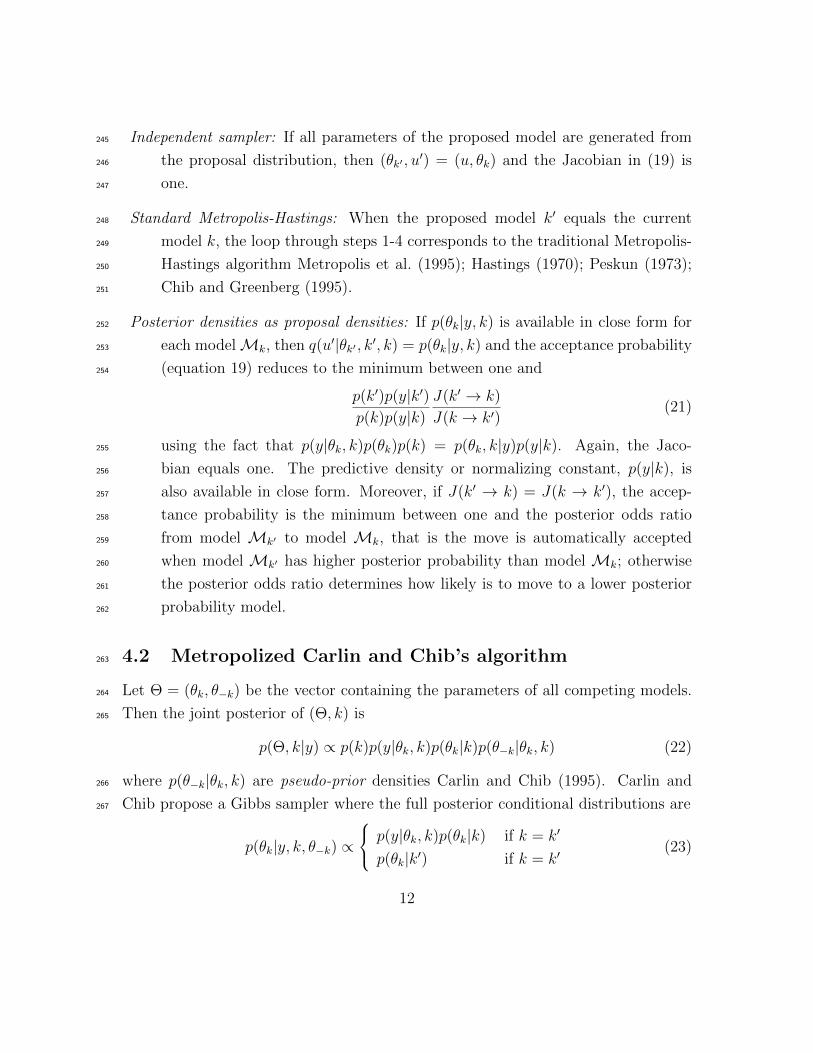
Independent sampler: If all parameters of the proposed model are generated from245

the proposal distribution, then (θk′ , u′) = (u, θk) and the Jacobian in (19) is246

one.247

Standard Metropolis-Hastings: When the proposed model k′ equals the current248

model k, the loop through steps 1-4 corresponds to the traditional Metropolis-249

Hastings algorithm Metropolis et al. (1995); Hastings (1970); Peskun (1973);250

Chib and Greenberg (1995).251

Posterior densities as proposal densities: If p(θk|y, k) is available in close form for252

each modelMk, then q(u′|θk′ , k′, k) = p(θk|y, k) and the acceptance probability253

(equation 19) reduces to the minimum between one and254

p(k′)p(y|k′)p(k)p(y|k)

J(k′ → k)

J(k → k′)(21)

using the fact that p(y|θk, k)p(θk)p(k) = p(θk, k|y)p(y|k). Again, the Jaco-255

bian equals one. The predictive density or normalizing constant, p(y|k), is256

also available in close form. Moreover, if J(k′ → k) = J(k → k′), the accep-257

tance probability is the minimum between one and the posterior odds ratio258

from model Mk′ to model Mk, that is the move is automatically accepted259

when model Mk′ has higher posterior probability than model Mk; otherwise260

the posterior odds ratio determines how likely is to move to a lower posterior261

probability model.262

4.2 Metropolized Carlin and Chib’s algorithm263

Let Θ = (θk, θ−k) be the vector containing the parameters of all competing models.264

Then the joint posterior of (Θ, k) is265

p(Θ, k|y) ∝ p(k)p(y|θk, k)p(θk|k)p(θ−k|θk, k) (22)

where p(θ−k|θk, k) are pseudo-prior densities Carlin and Chib (1995). Carlin and266

Chib propose a Gibbs sampler where the full posterior conditional distributions are267

p(θk|y, k, θ−k) ∝

p(y|θk, k)p(θk|k) if k = k′

p(θk|k′) if k = k′(23)

12

and268

p(k|Θ, y) ∝ p(y|θk, k)p(k)∏m∈M

p(θm|k) (24)

Notice that the pseudo-prior densities and the RJMCMC’s proposal densities269

have similar functions. As a matter of fact, Carlin and Chib suggest using pseudo-270

prior distributions that are close to the posterior distributions within each competing271

model.272

The main problem with Carlin and Chib’s Gibbs sampler is the need of evaluating273

and drawing from the pseudo-prior distributions at each iteration of the MCMC274

scheme. This problem can be overwhelmingly exacerbated in large situations where275

the number of competing models is relatively large (See Clyde, 1999, for applications276

and discussions in variable selection in regression models).277

To overcome this last problem Dellaportas et al. and Godsill (2001) proposes278

“Metropolizing” Carlin and Chib’s Gibbs sampler. If the current state of the Markov279

chain is at (θk, k), then they suggest proposing and accepting/rejecting a move to a280

new model in the following way:281

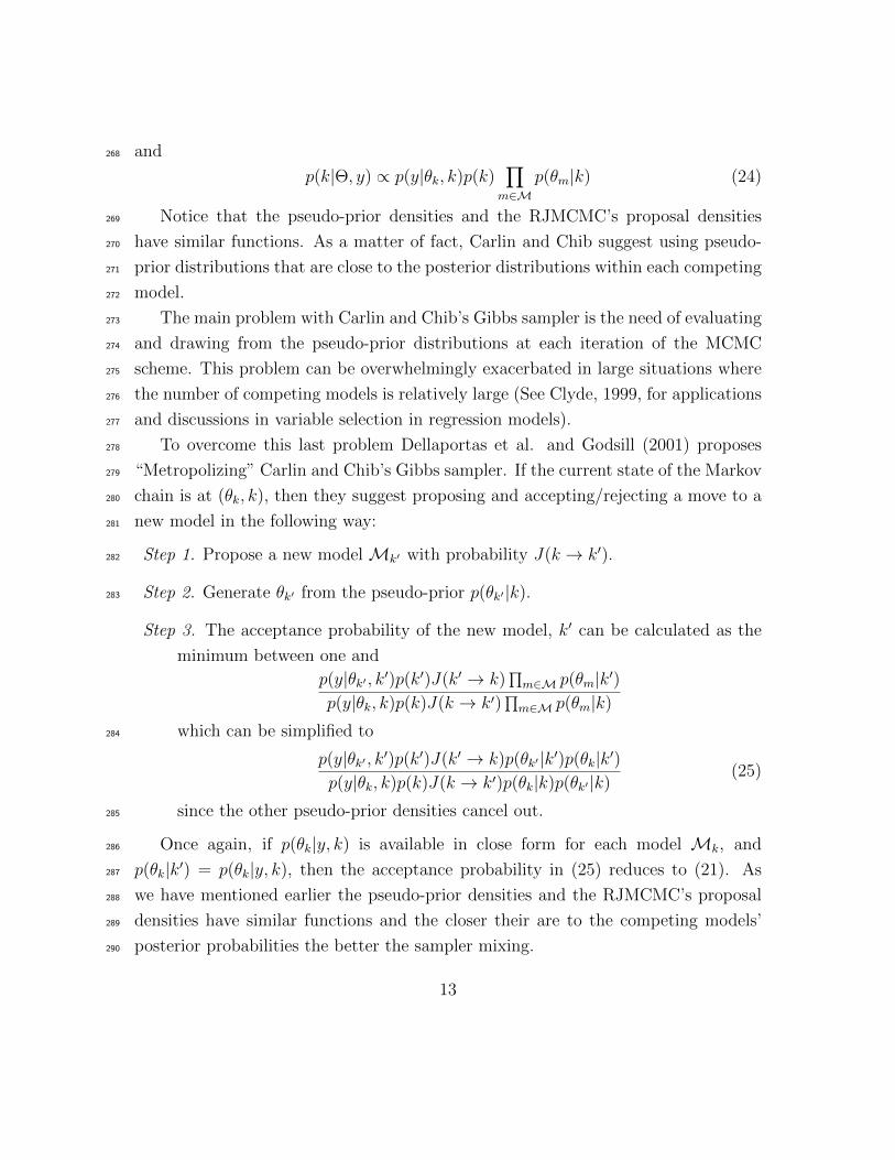
Step 1. Propose a new model Mk′ with probability J(k → k′).282

Step 2. Generate θk′ from the pseudo-prior p(θk′ |k).283

Step 3. The acceptance probability of the new model, k′ can be calculated as the

minimum between one and

p(y|θk′ , k′)p(k′)J(k′ → k)∏m∈M p(θm|k′)

p(y|θk, k)p(k)J(k → k′)∏m∈M p(θm|k)

which can be simplified to284

p(y|θk′ , k′)p(k′)J(k′ → k)p(θk′|k′)p(θk|k′)p(y|θk, k)p(k)J(k → k′)p(θk|k)p(θk′ |k)

(25)

since the other pseudo-prior densities cancel out.285

Once again, if p(θk|y, k) is available in close form for each model Mk, and286

p(θk|k′) = p(θk|y, k), then the acceptance probability in (25) reduces to (21). As287

we have mentioned earlier the pseudo-prior densities and the RJMCMC’s proposal288

densities have similar functions and the closer their are to the competing models’289

posterior probabilities the better the sampler mixing.290

13

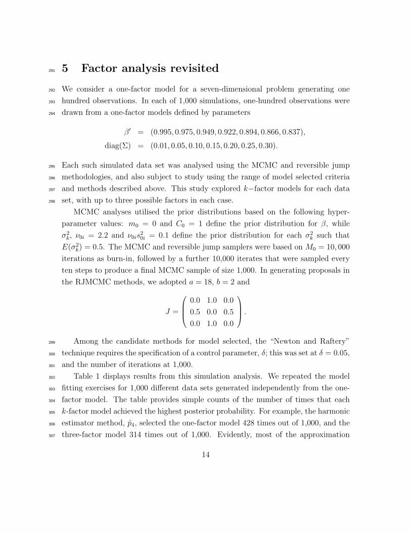
5 Factor analysis revisited291

We consider a one-factor model for a seven-dimensional problem generating one292

hundred observations. In each of 1,000 simulations, one-hundred observations were293

drawn from a one-factor models defined by parameters294

β′ = (0.995, 0.975, 0.949, 0.922, 0.894, 0.866, 0.837),

diag(Σ) = (0.01, 0.05, 0.10, 0.15, 0.20, 0.25, 0.30).

Each such simulated data set was analysed using the MCMC and reversible jump295

methodologies, and also subject to study using the range of model selected criteria296

and methods described above. This study explored k−factor models for each data297

set, with up to three possible factors in each case.298

MCMC analyses utilised the prior distributions based on the following hyper-

parameter values: m0 = 0 and C0 = 1 define the prior distribution for β, while

σ2k, ν0i = 2.2 and ν0is

20i = 0.1 define the prior distribution for each σ2

k such that

E(σ2k) = 0.5. The MCMC and reversible jump samplers were based on M0 = 10, 000

iterations as burn-in, followed by a further 10,000 iterates that were sampled every

ten steps to produce a final MCMC sample of size 1,000. In generating proposals in

the RJMCMC methods, we adopted a = 18, b = 2 and

J =

0.0 1.0 0.0

0.5 0.0 0.5

0.0 1.0 0.0

.Among the candidate methods for model selected, the “Newton and Raftery”299

technique requires the specification of a control parameter, δ; this was set at δ = 0.05,300

and the number of iterations at 1,000.301

Table 1 displays results from this simulation analysis. We repeated the model302

fitting exercises for 1,000 different data sets generated independently from the one-303

factor model. The table provides simple counts of the number of times that each304

k-factor model achieved the highest posterior probability. For example, the harmonic305

estimator method, p4, selected the one-factor model 428 times out of 1,000, and the306

three-factor model 314 times out of 1,000. Evidently, most of the approximation307

14

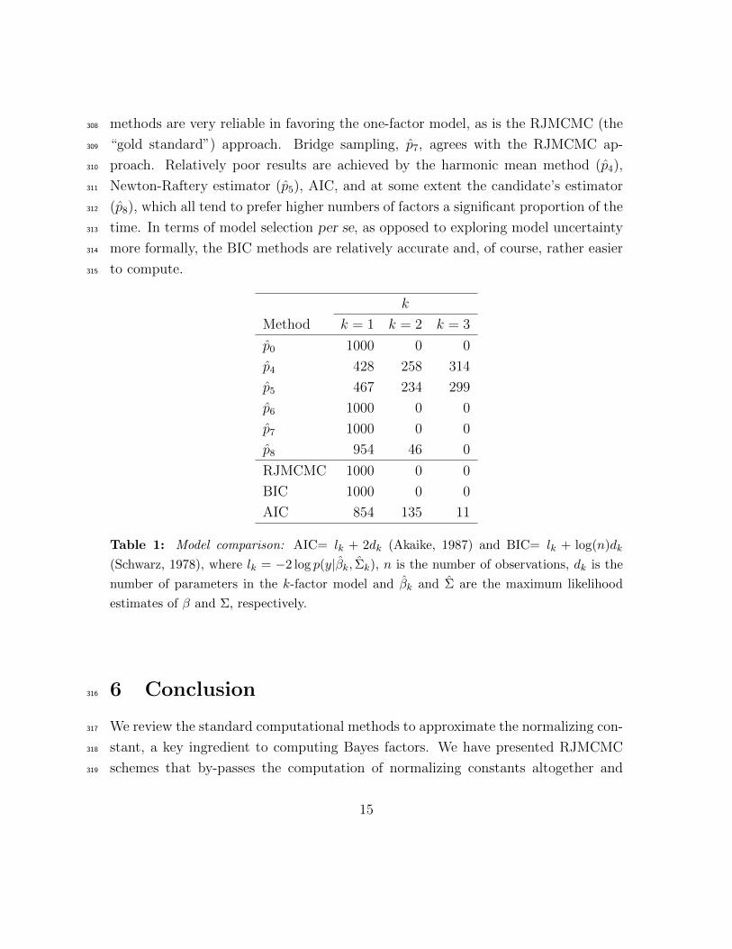
methods are very reliable in favoring the one-factor model, as is the RJMCMC (the308

“gold standard”) approach. Bridge sampling, p7, agrees with the RJMCMC ap-309

proach. Relatively poor results are achieved by the harmonic mean method (p4),310

Newton-Raftery estimator (p5), AIC, and at some extent the candidate’s estimator311

(p8), which all tend to prefer higher numbers of factors a significant proportion of the312

time. In terms of model selection per se, as opposed to exploring model uncertainty313

more formally, the BIC methods are relatively accurate and, of course, rather easier314

to compute.315

k

Method k = 1 k = 2 k = 3

p0 1000 0 0

p4 428 258 314

p5 467 234 299

p6 1000 0 0

p7 1000 0 0

p8 954 46 0

RJMCMC 1000 0 0

BIC 1000 0 0

AIC 854 135 11

Table 1: Model comparison: AIC= lk + 2dk (Akaike, 1987) and BIC= lk + log(n)dk

(Schwarz, 1978), where lk = −2 log p(y|βk, Σk), n is the number of observations, dk is the

number of parameters in the k-factor model and βk and Σ are the maximum likelihood

estimates of β and Σ, respectively.

6 Conclusion316

We review the standard computational methods to approximate the normalizing con-317

stant, a key ingredient to computing Bayes factors. We have presented RJMCMC318

schemes that by-passes the computation of normalizing constants altogether and319

15

directly approximate posterior model probabilities. We have used the standard nor-320

mal linear factor model as a motivational example to illustrate the implementation of321

such methods. For additional discussion on Bayes factors and their approximations322

for model comparison, see Kass and Raftery (1995), DiCiccio et al. (1997), Han and323

Carlin (2001), Kadane and Lazar (2004), Lopes and West (2004) and Chapter 7 of324

Gamerman and Lopes (2006), amongst others.325

References326

Akaike, H. (1987). Factor analysis and AIC. Psychometrika 52, 317–332.327

Amemiya, Y. and T. W. Anderson (1990). Asymptotic chi-square tests for a large328

class of factor analysis models. The Annals of Statistics 18, 1453–1463.329

Anderson, T. W. and Y. Amemiya (1988). The asymptotic normal distribution of330

estimators in factor analysis under general conditions. The Annals of Statistics 16,331

759–771.332

Anderson, T. W. and H. Rubin (1956). Statistical inference in factor analysis. In333

J. Neyman (Ed.), Proceedings of the Third Berkeley Symposium of Mathematical334

Statistics and Probability, Volume 5, pp. 111–150. University of California Press,335

Berkeley.336

Barbieri, M. and A. O’Hagan (1996). A reversible jump MCMC sampler for337

Bayesian analysis of ARMA time series. Technical report, Dipartimento di Statis-338

tica,Probabilita e Statistiche Applicate, Universita La Sapienza,Roma.339

Bentler, P. M. and J. S. Tanaka (1983). Problems with EM algorithms for ML factor340

analysis. Psychometrika 48, 247–251.341

Besag, J. (1989). A candidate’s formula: A curious result in Bayesian prediction.342

Biometrika 76, 183–183.343

Burt, C. (1940). The Factors of the Mind: An Introduction to Factor Analysis in344

Psychology. University of London Press, London.345

16

Carlin, B. and S. Chib (1995). Bayesian model choice via Markov chain Monte Carlo346

methods. Journal of the Royal Statistical Society, B 57, 473–484.347

Chen, M.-H., Q.-M. Shao, and J. Ibrahim (2000). Monte Carlo methods in Bayesian348

computation. New York: Springer-Verlag.349

Chib, S. (1995). Marginal likelihood from the Gibbs output. Journal of the American350

Statistical Association 90, 1313–1321.351

Chib, S. and E. Greenberg (1995). Understanding the Metropolis-Hastings algorithm.352

The American Statistician 49, 327–335.353

Chib, S. and I. Jeliazkov (2001). Marginal likelihood from the Metropolis-Hastings354

output. Journal of the American Statistical Association 96, 270–281.355

Chib, S. and I. Jeliazkov (2005). Accept-reject Metropolis-Hastings sampling and356

marginal likelihood estimation. Statistica Neerlandica 59, 30–44.357

Clyde, M. (1999). Bayesian model averaging and model search strategies (with dis-358

cussion). In J. Bernardo, J. Berger, A. Dawid, and A. Smith (Eds.), Bayesian359

Statistics 6, pp. 157–185. John Wiley.360

Cudeck, R. and R. C. MacCallum (2007). Factor Analysis at 100: Historical Devel-361

opments and Future Directions. Routledge.362

Dellaportas, P., J. Forster, and I. Ntzoufras (2002). On Bayesian model and variable363

selection using MCMC. Statistics and Computing 12, 27–36.364

Denison, D. G. T., B. K. Mallick, and A. F. M. Smith (1998). Automatic Bayesian365

curve fitting. Journal of the Royal Statistical Society. Series B 60, 333–350.366

DiCiccio, T., R. Kass, A. Raftery, and L. Wasserman (1997). Computing Bayes’367

factors by combining simulation and asymptotic approximations. Journal of the368

American Statistical Association 92, 903–915.369

Gamerman, D. and H. F. Lopes (2006). Markov Chain Monte Carlo - Stochastic370

Simulation for Bayesian Inference (2nd ed.). Chapman&Hall/CRC.371

17

Gelfand, A. and D. Dey (1994). Bayesian model choice: Asymptotics and exact372

calculations. Journal of the Royal Statistical Society, Ser. B 56, 501–514.373

Gelman, A. and X. L. Meng (1997). On monte carlo methods for estimating ratios374

of normalizing constants. Annals of Statistics 25, 1563–1594.375

Gelman, A. and X. L. Meng (1998). Simulating normalizing constants: From im-376

portance sampling to bridge sampling to path sampling. Statistical Science 13,377

163–185.378

Geweke, J. and G. Zhou (1996). Measuring the pricing error of the arbitrage pricing379

theory. The Review of Financial Studies 9, 557–587.380

Godsill, S. J. (2001). On the relationship between Markov chain Monte Carlo381

methods for model uncertainty. Journal of Computational and Graphical Statis-382

tics 10 (2), 230–248.383

Green, P. (1995). Reversible jump Markov chain Monte Carlo computation and384

Bayesian model determination. Biometrika 82, 711–732.385

Han, C. and B. P. Carlin (2001). Markov chain monte carlo methods for computing386

bayes factors: A comparative review. Journal of the American Statistical Associ-387

ation 96, 1122–1132.388

Hastings, W. (1970). Monte Carlo sampling methods using Markov chains and their389

applications. Biometrika 57, 97–109.390

Holzinger, K. J. and H. H. Harman (1941). Factor analysis: A Synthesis of Factorial391

Methods. University of Chicago Press, Chicago.392

Hotelling, H. (1955). Analysis of a complex of statistical variables into principal393

components. Journal of Educational Psychology 24, 417–441.394

Huerta, G. and H. F. Lopes (2000). Bayesian forecasting and inference in latent395

structure for the Brazilian industrial production index. Brazilian Review of Econo-396

metrics 20, 1–26.397

18

Huerta, G. and M. West (1999). Priors and component structures in autoregressive398

time series models. Journal of the Royal Statistical Society-Series B 61, 881–899.399

Jeffreys, H. (1961). Theory of Probability (3rd edition). Oxford University Press.400

Joreskog, K. (1967). Some contributions to maximum likelihood factor analysis.401

Psychometrika 32, 443–482.402

Joreskog, K. G. (1969). A general approach to confirmatory maximum likelihood403

factor analysis. Psychometrika 34, 183–220.404

Kadane, J. B. and N. A. Lazar (2004). Methods and criteria for model selection.405

Journal of the American Statistical Association 99, 279–290.406

Kass, R. and A. Raftery (1995). Bayes’ factor. Journal of the American Statistical407

Association 90, 773–795.408

Lawley (1940). The estimation of factor loadings by the method of maximum likeli-409

hood. Proceedings of the Royal Society of Edinburgh 60, 64–82.410

Lawley (1953). Further investigations in factor estimation. Proceedings of the Royal411

Society of Edinburgh 60, 64–82.412

Lewis, S. and A. Raftery (1997). Estimating Bayes’ factors via posterior simula-413

tion with the Laplace-Metropolis estimator. Journal of the American Statistical414

Association 92, 648–655.415

Lopes, H. F. (2014). Modern bayesian factor analysis. In I. Jeliazkov and X.-S. Yang416

(Eds.), Bayesian inference in the Social Sciences. Wiley.417

Lopes, H. F., E. Salazar, and D. Gamerman (2008). Spatial dynamic factor models.418

Bayesian Analysis 5, 1–30.419

Lopes, H. F. and M. West (2004). Bayesian model assessment in factor analysis.420

Statistica Sinica 14, 41–67.421

Meng, X. and W. Wong (1996). Simulating ratios of normalizing constants via a422

simple identity: A theoretical exploration. Statistica Sinica 6, 831–860.423

19

Meng, X. L. and S. Schilling (1996). Fitting full-information factor models and an424

empirical investigation of bridge sampling. Journal of the American Statistical425

Association 91, 1254–1267.426

Meng, X.-L. and S. Schilling (2002). Warp bridge sampling. Journal of Computational427

and Graphical Statistics 11, pp. 552–586.428

Metropolis, N., A. Rosenbluth, M. Rosenbluth, and A. Teller (1995). Equations of429

state calculations by fast computing machines. Journal of Chemical Physics 21,430

1087–1092.431

Mira, A. and G. K. Nicholls (2004). Bridge estimation of the probability density at432

a point. Statistica Sinica 14, 603–612.433

Newton, M. and A. Raftery (1994). Approximate Bayesian inference with the434

weighted likelihood bootstrap. Journal of the Royal Statistical Society, Ser. B 56,435

3–48.436

Peskun, P. (1973). Optimum Monte-Carlo sampling using Markov chains.437

Biometrika 60, 607–612.438

Raftery, A. (1996). Hypothesis testing and model selection. In W. Gilks, S. Richard-439

son, and D. Spiegelhalter (Eds.), Markov Chain Monte Carlo in Practice. Chapman440

and Hall.441

Richardson, S. and P. Green (1997). Reversible jump Markov chain Monte Carlo442

computation and Bayesian model determination (with discussion). Journal of the443

Royal Statistical Society - Series B 59, 731–758.444

Rubin, D. B. and D. T. Thayer (1982). EM algorithms for ML factor analysis.445

Psychometrika 47, 69–76.446

Rubin, D. B. and D. T. Thayer (1983). More on the EM for factor analysis. Psy-447

chometrika 48, 253–257.448

Schwarz, G. (1978). Estimating the dimension of a model. The Annals of Statistics 6,449

461–464.450

20

Spearman (1904). General intelligence objectively determined and measured. Amer-451

ican Journal of Psychology 15, 201–292.452

Thomson, G. H. (1953). The Factor Analysis of Human Ability. University of London453

Press, London.454

Thurstone, L. (1947). Multiple Factor Analysis. University of Chicago Press.455

Thurstone, L. L. (1935). Vectors of the Mind. University of Chicago Press, Chicago.456

Wolpert, R. L. and S. C. Schmidler (2012). α-stable limit laws for harmonic mean457

estimators of marginal likelihoods. Statistica Sinica 22, 1233–1251.458

21