http://www.biological-networks.org

Dr Marcus Kaiser

A Tutorial in Connectome Analysis (III): Topological and Spatial Features of Brain Networks

School of Computing Science /

Institute of Neuroscience Newcastle University

United Kingdom

WCU Dept of Brain & Cognitive Sciences Seoul National University South Korea http://bcs.snu.ac.kr/

1

2

Brain connectivity

Hilgetag & Kaiser (2004) Neuroinformatics 2: 353

Types of Brain Connectivity Structural, functional, effective Small-world Neighborhood clustering Shortest path length Spatial preference for short connections but more long-distance connections than expected Structure->Function Network changes lead to cognitive deficits (Alzheimer’s disease, IQ)

3

Outline Microscale (one component) •  Centrality measures

Mesoscale (several components) •  Motifs •  Clusters Macroscale (all components) •  Degree distributions:

Random and Scale-free networks

Studying network robustness

Centrality measures

4

5

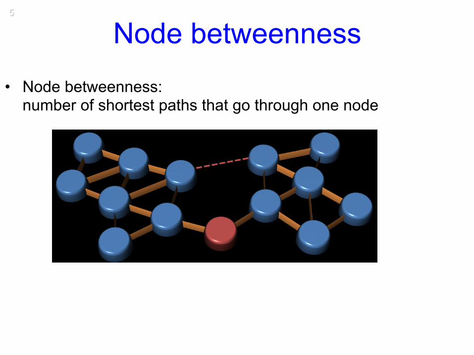
Node betweenness

•  Node betweenness: number of shortest paths that go through one node

6

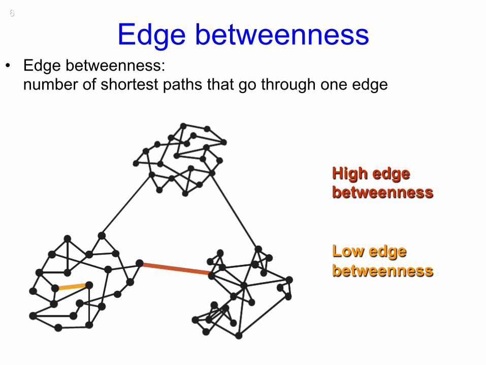
Edge betweenness •  Edge betweenness:

number of shortest paths that go through one edge

High edge betweenness Low edge betweenness

7

Centrality measure example

Node 8 has the highest node betweenness Edge 8-9 has the highest edge betweenness

Motifs

8

9

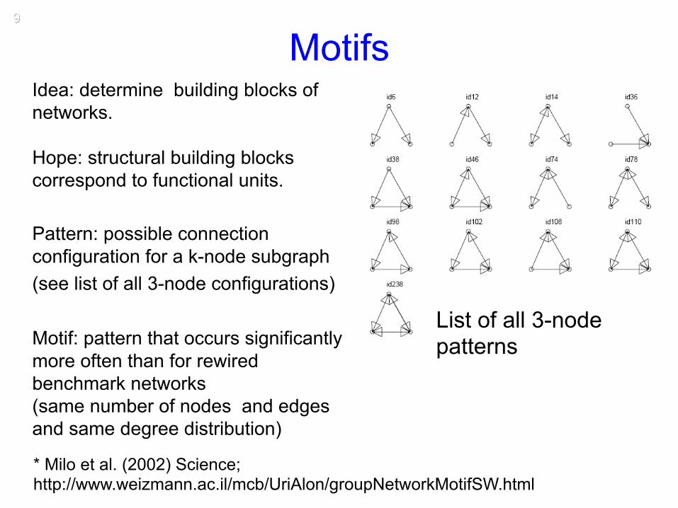
Motifs Idea: determine building blocks of networks. Hope: structural building blocks correspond to functional units. Pattern: possible connection configuration for a k-node subgraph (see list of all 3-node configurations)

Motif: pattern that occurs significantly more often than for rewired benchmark networks (same number of nodes and edges and same degree distribution)

* Milo et al. (2002) Science; http://www.weizmann.ac.il/mcb/UriAlon/groupNetworkMotifSW.html

List of all 3-node patterns

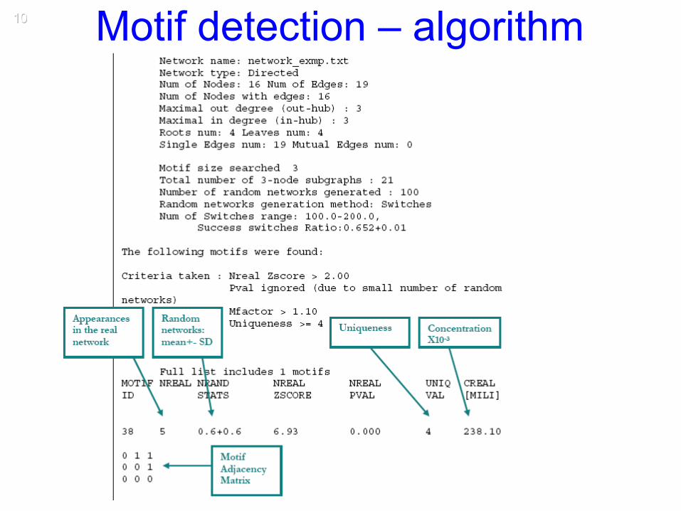
10 Motif detection – algorithm

11

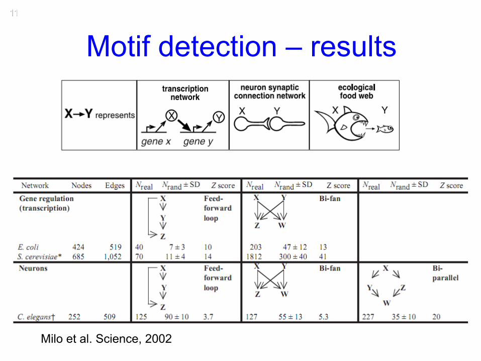
Motif detection – results

Milo et al. Science, 2002

12

Motif detection – problems Advantages: -  Identify special network patterns which might represent functional modules

Disadvantages: - Slow for large networks and

unfeasible for large (e.g. 5-node) motifs (#patterns: 3-node – 13; 4-node – 199; 5-node: 9364; 6-node - 1,530,843)

- Rewired benchmark networks do not retain clusters; most patterns become insignificant for clustered benchmark networks*

* Kaiser (2011) Neuroimage

13

Clusters (or Modules or Communities)

14

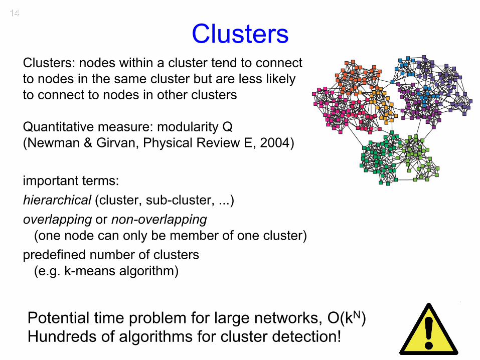
Clusters Clusters: nodes within a cluster tend to connect to nodes in the same cluster but are less likely to connect to nodes in other clusters Quantitative measure: modularity Q (Newman & Girvan, Physical Review E, 2004) important terms: hierarchical (cluster, sub-cluster, ...) overlapping or non-overlapping (one node can only be member of one cluster) predefined number of clusters (e.g. k-means algorithm)

Potential time problem for large networks, O(kN) Hundreds of algorithms for cluster detection!

15

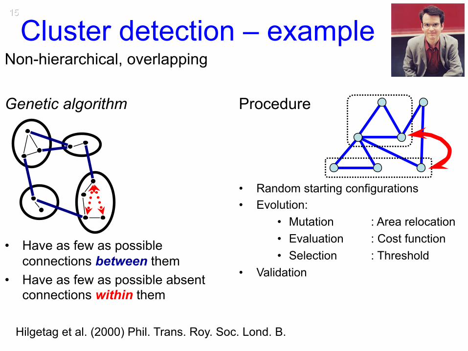
Cluster detection – example Non-hierarchical, overlapping Genetic algorithm Procedure

Hilgetag et al. (2000) Phil. Trans. Roy. Soc. Lond. B.

•  Have as few as possible connections between them

•  Have as few as possible absent connections within them

•  Random starting configurations •  Evolution:

•  Mutation : Area relocation •  Evaluation : Cost function •  Selection : Threshold

•  Validation

16

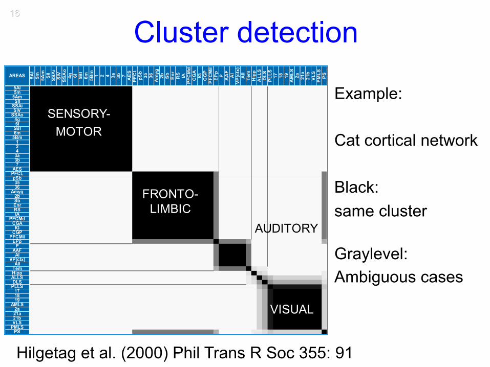
Cluster detection

Example: Cat cortical network Black: same cluster

Graylevel: Ambiguous cases

Hilgetag et al. (2000) Phil Trans R Soc 355: 91

AREAS 5Al

5m 5Am

SII

SSAi

SIV

SSAo

4g 6l

5Bl

6m 5Bm 1 2 4 3a 3b 7 AES

PFCL

pSb

35 36Amyg

2b Sb

Enr RS IA

PFCMd

CGA

IG CGP

PFCMil

EPpP AAF

AI

VP(ctx)

AII

Tem

Hipp

ALLS

DLS

PLLS

17 18 19AMLS2a 21a

21b

VLS

PMLSPS

5Al5m5AmSIISSAiSIVSSAo4g6l5Bl6m5Bm1243a3b7AESPFCLpSb3536

Amyg2bSbEnrRSIA

PFCMdCGAIGCGPPFCMilEPpPAAFAI

VP(ctx)AIITemHippALLSDLSPLLS171819

AMLS2a21a21bVLSPMLSPS

VISUAL

AUDITORY

FRONTO-LIMBIC

SENSORY-MOTOR

Random graphs

17

18

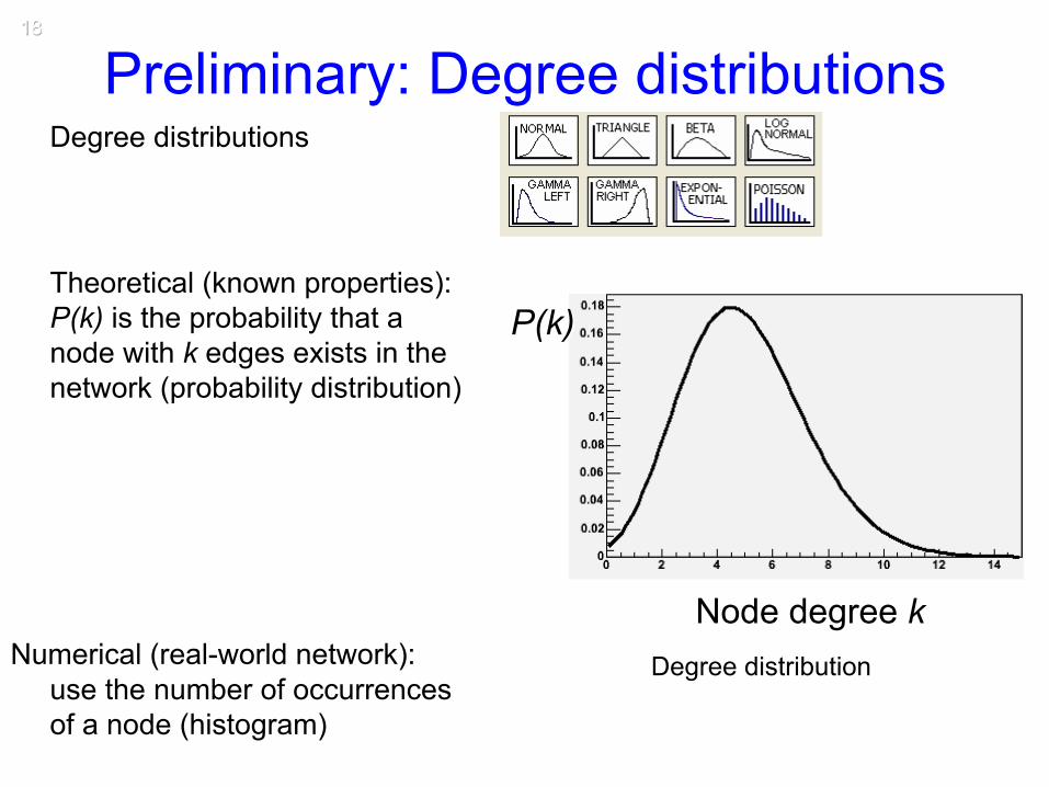
Preliminary: Degree distributions Degree distributions

Theoretical (known properties): P(k) is the probability that a node with k edges exists in the network (probability distribution)

Numerical (real-world network): use the number of occurrences of a node (histogram)

P(k)

Node degree k Degree distribution

19

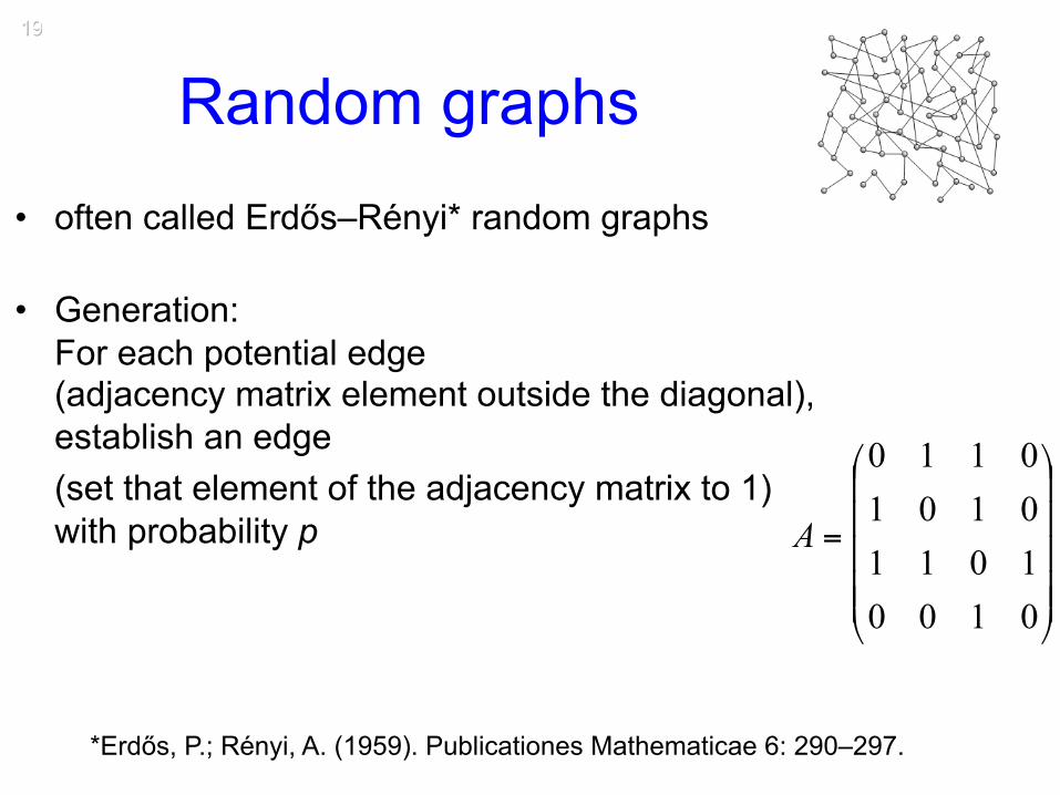
Random graphs •  often called Erdős–Rényi* random graphs

•  Generation:

For each potential edge (adjacency matrix element outside the diagonal), establish an edge (set that element of the adjacency matrix to 1) with probability p

*Erdős, P.; Rényi, A. (1959). Publicationes Mathematicae 6: 290–297.

⎟⎟⎟⎟⎟

⎠

⎞

⎜⎜⎜⎜⎜

⎝

⎛

=

0100101101010110

A

20

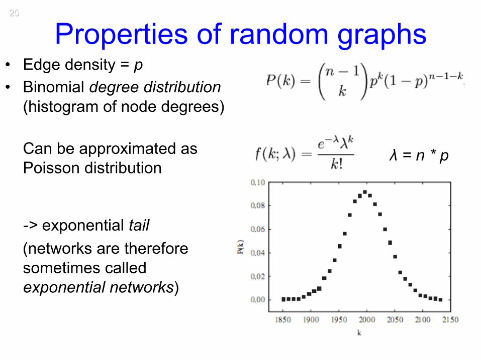
Properties of random graphs •  Edge density = p •  Binomial degree distribution

(histogram of node degrees)

Can be approximated as Poisson distribution -> exponential tail

(networks are therefore sometimes called exponential networks)

λ = n * p

Scale-free networks

21

22

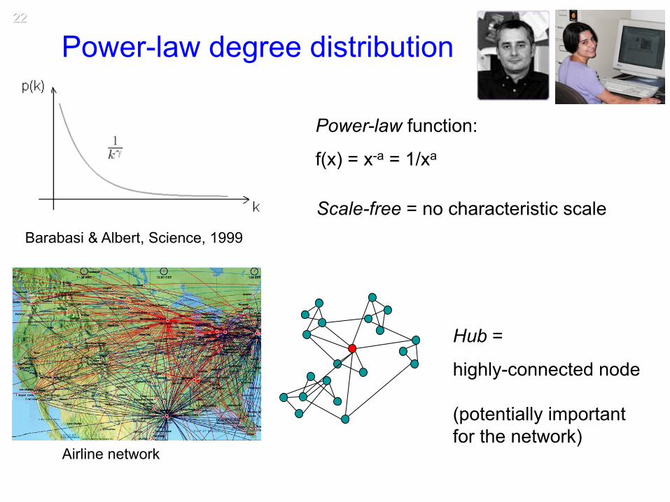
Scale-free = no characteristic scale

Power-law degree distribution

Barabasi & Albert, Science, 1999

Hub =

highly-connected node (potentially important for the network)

Airline network

Power-law function:

f(x) = x-a = 1/xa

23

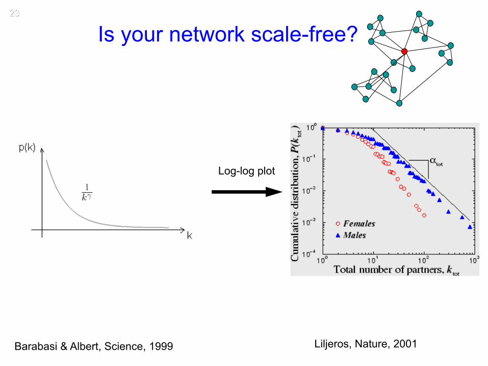
Is your network scale-free?

Barabasi & Albert, Science, 1999 Liljeros, Nature, 2001

Log-log plot

24

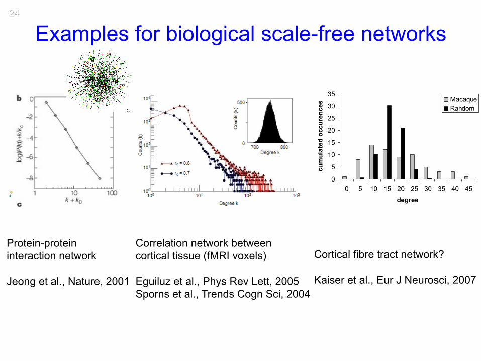
Examples for biological scale-free networks

Protein-protein interaction network Jeong et al., Nature, 2001

Correlation network between cortical tissue (fMRI voxels) Eguiluz et al., Phys Rev Lett, 2005 Sporns et al., Trends Cogn Sci, 2004

Cortical fibre tract network? Kaiser et al., Eur J Neurosci, 2007

0

5

10

15

20

25

30

35

0 5 10 15 20 25 30 35 40 45

degree

cum

ulat

ed o

ccur

ence

s MacaqueRandom

Robustness

25

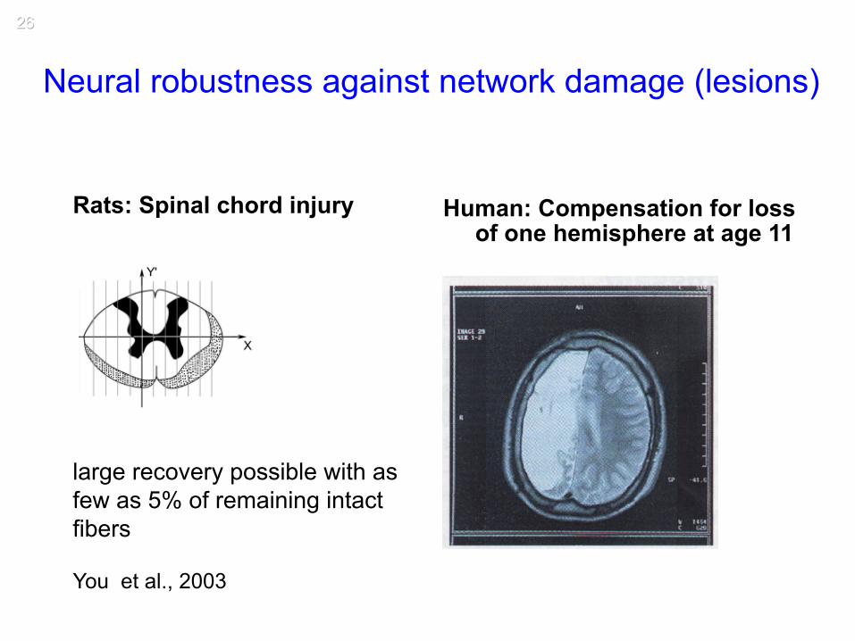
Neural robustness against network damage (lesions)

You et al., 2003

Rats: Spinal chord injury

large recovery possible with as few as 5% of remaining intact fibers

Human: Compensation for loss of one hemisphere at age 11

26

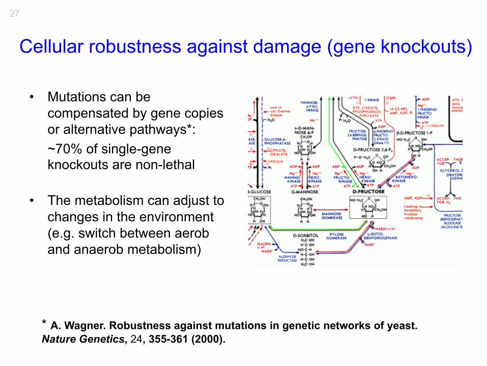
•  Mutations can be compensated by gene copies or alternative pathways*: ~70% of single-gene knockouts are non-lethal

•  The metabolism can adjust to changes in the environment (e.g. switch between aerob and anaerob metabolism)

* A. Wagner. Robustness against mutations in genetic networks of yeast. Nature Genetics, 24, 355-361 (2000).

Cellular robustness against damage (gene knockouts)

27

28

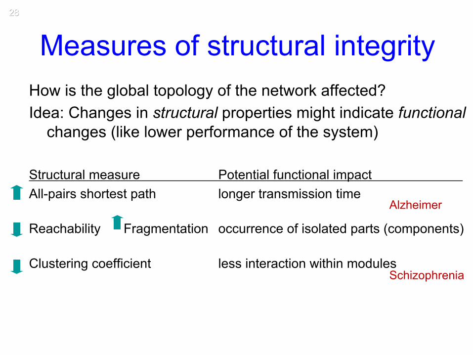
Measures of structural integrity How is the global topology of the network affected? Idea: Changes in structural properties might indicate functional

changes (like lower performance of the system) Structural measure Potential functional impact . All-pairs shortest path longer transmission time

Reachability Fragmentation occurrence of isolated parts (components)

Clustering coefficient less interaction within modules

Alzheimer Schizophrenia

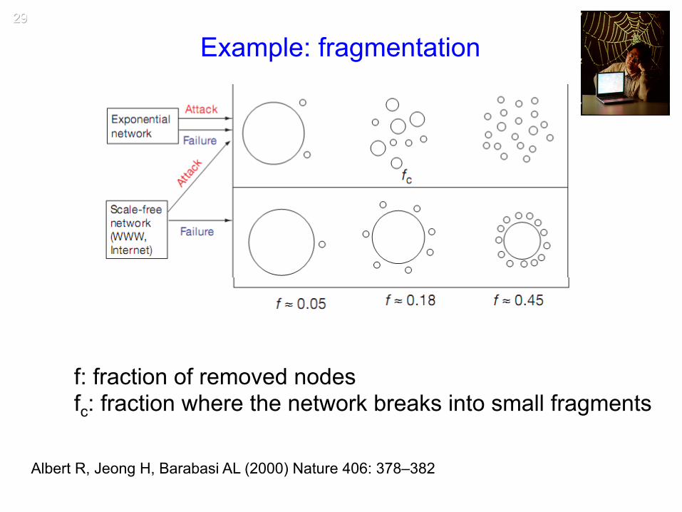
Albert R, Jeong H, Barabasi AL (2000) Nature 406: 378–382

Example: fragmentation

f: fraction of removed nodes fc: fraction where the network breaks into small fragments

29

30

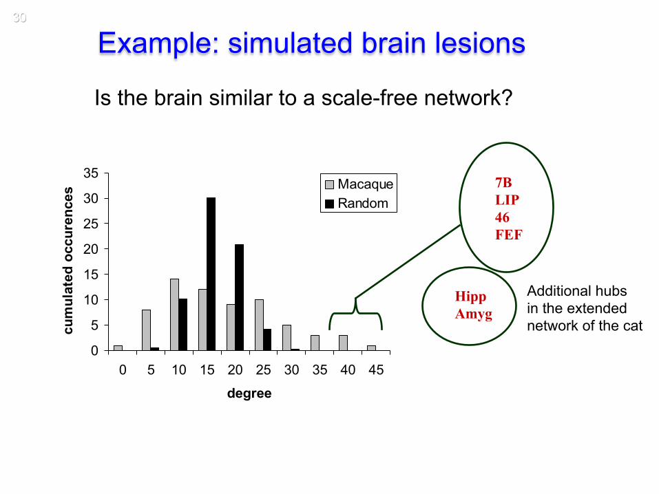
Example: simulated brain lesions

0

5

10

15

20

25

30

35

0 5 10 15 20 25 30 35 40 45

degree

cum

ulat

ed o

ccur

ence

s MacaqueRandom

Hipp Amyg

Additional hubs in the extended network of the cat

7B LIP 46 FEF

Is the brain similar to a scale-free network?

31

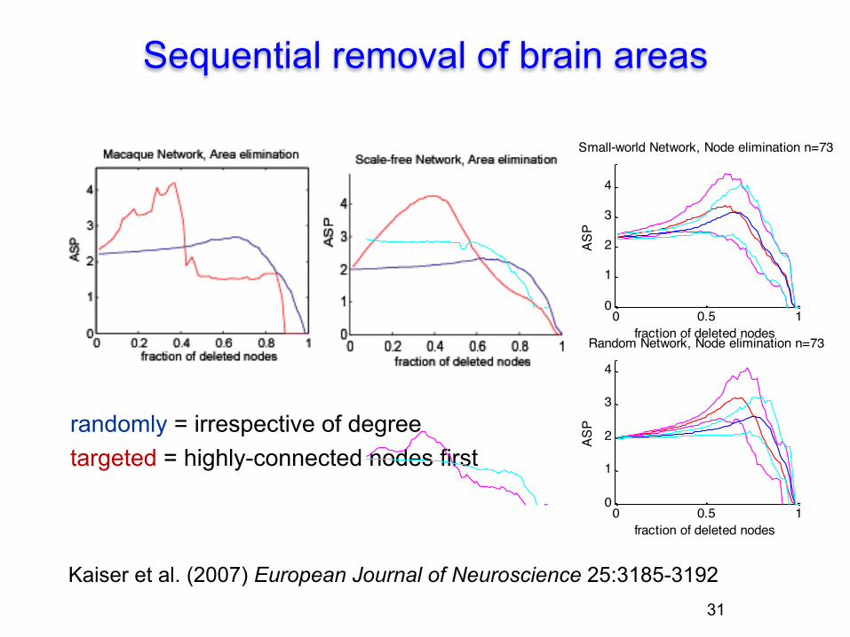
Sequential removal of brain areas

randomly = irrespective of degree targeted = highly-connected nodes first

Kaiser et al. (2007) European Journal of Neuroscience 25:3185-3192

0 0.5 10

1

2

3

4

fraction of deleted nodesAS

P

Cortical Network, Node elimination n=73

0 0.5 10

1

2

3

4

fraction of deleted nodes

ASP

Small-world Network, Node elimination n=73

0 0.5 10

1

2

3

4

fraction of deleted nodes

ASP

Random Network, Node elimination n=73

0 0.5 10

2

4

6

fraction of deleted nodes

ASP

Scale-free Network, Node elimination n=73

32

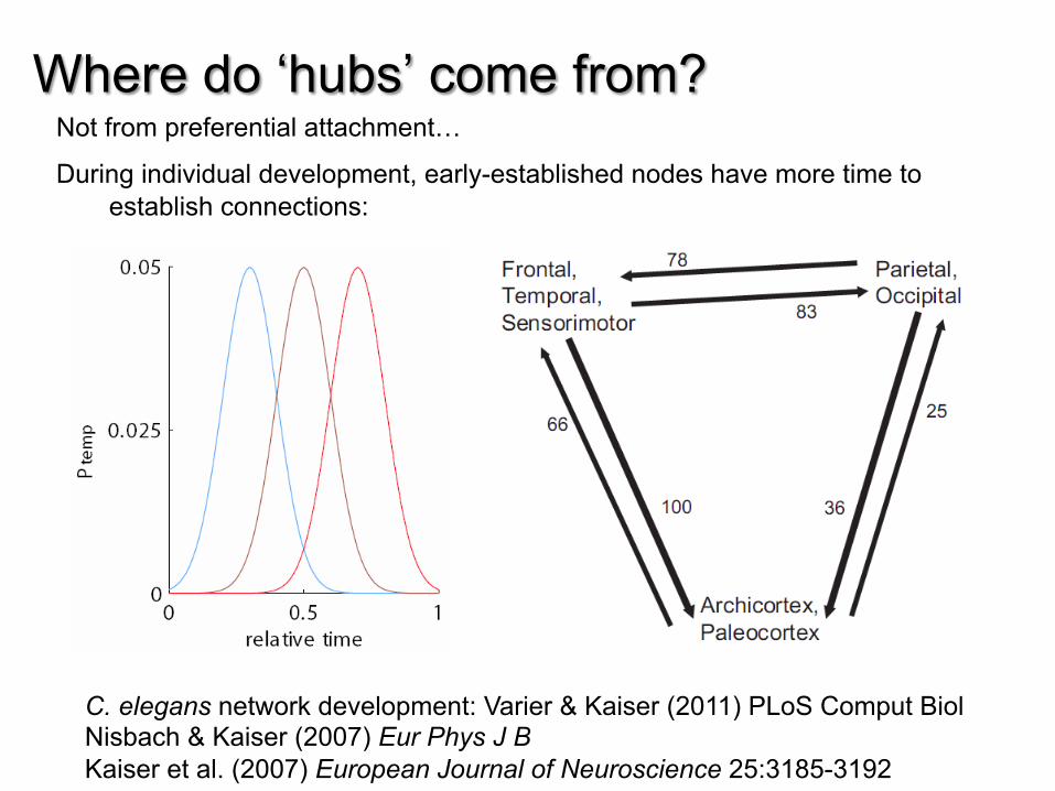
Where do ‘hubs’ come from? Not from preferential attachment…

During individual development, early-established nodes have more time to establish connections:

C. elegans network development: Varier & Kaiser (2011) PLoS Comput Biol Nisbach & Kaiser (2007) Eur Phys J B Kaiser et al. (2007) European Journal of Neuroscience 25:3185-3192

33

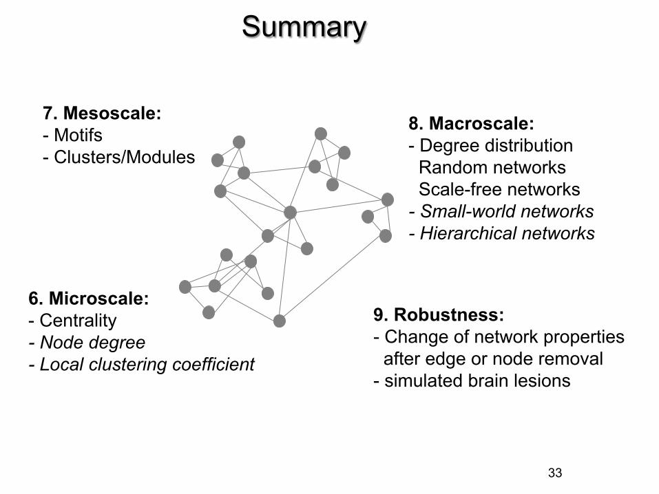
Summary

6. Microscale: - Centrality - Node degree - Local clustering coefficient

7. Mesoscale: - Motifs - Clusters/Modules

8. Macroscale: - Degree distribution Random networks Scale-free networks - Small-world networks - Hierarchical networks

9. Robustness: - Change of network properties after edge or node removal - simulated brain lesions

34 Further readings

Costa et al. Characterization of Complex Networks Advances in Physics, 2006

Bullmore & Sporns. Complex Brain Networks Nature Reviews Neuroscience, 2009

Kaiser et al. Simulated Brain Lesions (brain as scale-free network) European Journal of Neuroscience, 2007 Alstott et al. Modeling the impact of lesions in the human brain PLoS Computational Biology, 2009

Malcolm Young

Ed Bullmore Olaf Sporns

Luciano da Fontoura Costa