Embed Size (px)
Citation preview
Fundamenta Informaticae XXI (2001) 1001–1032 1001
IOS Press
A tutorial implementationof a dependently typed lambda calculus
Andres LohUtrecht [email protected]
Conor McBrideUniversity of [email protected]
Wouter SwierstraUniversity of [email protected]
Abstract. We present the type rules for a dependently typed core calculus together with a straight-forward implementation in Haskell. We explicitly highlight the changes necessary to shift from asimply-typed lambda calculus to the dependently typed lambda calculus. We also describe how toextend our core language with data types and write several small example programs. The article isaccompanied by an executable interpreter and example code that allows immediate experimentationwith the system we describe.
1. Introduction
Most functional programmers are hesitant to program with dependent types. It is said that type checkingbecomes undecidable; the type checker will always loop; and that dependent types are just really, really,hard.
The same programmers, however, are perfectly happy to program with a ghastly hodgepodge ofcomplex type system extensions. Current Haskell implementations, for instance, support generalized al-gebraic data types, multi-parameter type classes with functional dependencies, associated types and typefamilies, impredicative higher-ranked types, and there are even more extensions on the way. Program-mers seem to be willing to go to great lengths just to avoid dependent types.
One of the major barriers preventing the further proliferation of dependent types is a lack of under-standing amongst the general functional programming community. While, by now, there are quite a fewgood experimental tools and programming languages based on dependent types, it is hard to grasp how
1002 A. Loh, C. McBride, W. Swierstra / A tutorial implementation of a dependently typed lambda calculus
these tools actually work. A significant part of the literature available on dependent types is written bytype theorists for other type theorists to read. As a result, these papers are often not easily accessibleto functional programmers. This article aims to remedy this situation by making the following novelcontributions:
• Most importantly, we aim to fill the just described gap in the literature. To set the scene, we studythe simply-typed lambda calculus (Section 2). We present both the mathematical specification andHaskell implementation of the abstract syntax, evaluation, and type checking. Taking the simply-typed lambda calculus as starting point, we move on to a minimal dependently typed lambdacalculus (Section 3).
Inspired by Pierce’s incremental development of type systems [19], we highlight the changes, bothin the specification and implementation, that are necessary to shift to the dependently typed lambdacalculus. Perhaps surprisingly, the modifications necessary are comparatively small. By makingthese changes as explicit as possible, we hope that the transition to dependent types will be assmooth as possible for readers already familiar with the simply-typed lambda calculus.
While none of the type systems we implement are new, we believe that our article can serve as agentle introduction on how to implement a dependently typed system in Haskell. Implementinga type system is one of the best ways to learn about all the subtle issues involved. Although wedo not aim to survey all the different ways to implement a typed lambda calculus, we do try to beexplicit about our design decisions, carefully mention alternative choices, and provide an outlineof the wider design space.
The full power of dependent types can only come to its own if we add data types to this basecalculus. Therefore we demonstrate how to extend our language with natural numbers and vectorsin Section 4. More data types can be added using the principles explained in this section. Usingthe added data types, we write the classic vector append operation to illustrate how to program inour core calculus.
• We briefly sketch how a programming language may be built on top of the core calculus (Sec-tion 5), which itself has the nature of an internal language: it is explicitly typed; it requires a lot ofcode that one would like to omit in real programs; it lacks a lot of syntactic sugar.
We feel that being so explicit does have merits: writing simple programs in the core calculus can bevery instructive and reveals a great deal about the behaviour of dependently typed systems. Learn-ing this core language can help understand the subtle differences between existing dependentlytyped systems. Writing larger programs directly in this calculus, however, is a pain. We thereforesketch some of the language concepts that are required to go from the core language toward a fullprogramming language.
• Finally, we have made it easy to experiment with our system: the source code of this articlecontains a small interpreter for the type system and evaluation rules we describe. By using thesame sources as the article, the interpreter is guaranteed to follow the implementation we describeclosely, and is carefully documented. It hence provides a valuable platform for further educationand experimentation.
A. Loh, C. McBride, W. Swierstra / A tutorial implementation of a dependently typed lambda calculus 1003
This article is not an introduction to dependently typed programming or an explanation on how toimplement a full dependently typed programming language. However, we hope that this article will helpto dispel many misconceptions functional programmers may have about dependent types, and that it willencourage readers to explore this exciting area of research further.
2. Simply Typed Lambda Calculus
On our journey to dependent types, we want to start on familiar ground. In this section, we thereforeconsider the simply-typed lambda calculus, or λ→ for short. In a sense, λ→ is the smallest imaginablestatically typed functional language. Every term is explicitly typed and no type inference is performed. Ithas a much simpler structure than the type lambda calculi at the basis of languages such as ML or Haskellthat support polymorphic types and type constructors. In λ→, there are only base types and functionscannot be polymorphic. Without further additions, λ→ is strongly normalizing: evaluation terminates forany term, independent of the evaluation strategy.
2.1. Abstract syntax
The type language of λ→ consists of just two constructs:
τ ::= α base type| τ → τ ′ function type
There is a set of base types α; compound types τ → τ ′ correspond to functions from τ to τ ′.
e ::= e :: τ annotated term1
| x variable| e e′ application| λx→ e lambda abstraction
There are four kinds of terms: terms with an explicit type annotation; variables; applications; and lambdaabstractions.
Terms can be evaluated to values:
v ::= n neutral term| λx→ v lambda abstraction
n ::= x variable| n v application
A value is either a neutral term, i.e., a variable applied to a (possibly empty) sequence of values, or it isa lambda abstraction.
1Type theorists use ‘:’ or ‘∈’ to denote the type inhabitation relation. In Haskell, the symbol ‘:’ is used as the “cons” operatorfor lists, therefore the designers of Haskell chose the non-standard ‘::’ for type annotations. In this article, we will stick as closeas possible to Haskell’s syntax, in order to reduce the syntactic gap between the languages involved in the presentation.
1004 A. Loh, C. McBride, W. Swierstra / A tutorial implementation of a dependently typed lambda calculus
e ⇓ ve :: τ ⇓ v x ⇓ x
e ⇓ λx→ v e′ ⇓ v′
e e′ ⇓ v[x 7→ v′ ]e ⇓ n e′ ⇓ v′
e e′ ⇓ n v′e ⇓ v
λx→ e ⇓ λx→ v
Figure 1. Evaluation in λ→
2.2. Evaluation
The (big-step) evaluation rules of λ→ are given in Figure 1. The notation e ⇓ v means that the result ofcompletely evaluating e is v. Since we are in a strongly normalizing language, the evaluation strategy isirrelevant. To keep the presentation simple, we evaluate everything as far as possible, and even evaluateunder lambda. Type annotations are ignored during evaluation. Variables evaluate to themselves. Theonly interesting case is application. In that case, it depends whether the left hand side evaluates to alambda abstraction or to a neutral term. In the former case, we β-reduce. In the latter case, we add theadditional argument to the spine.
Here are few example terms in λ→, and their evaluations. Let us write id to denote the term λx→ x,and const to denote the term λx y→ x, which we use in turn as syntactic sugar for λx→ λy→ x. Then
(id :: α→ α) y ⇓ y
(const :: (β → β)→ α→ β → β) id y ⇓ id
2.3. Type System
Type rules are generally of the form 0 ` e::t, indicating that a term e is of type t in context 0. The contextlists valid base types, and associates identifiers with type information. We write α ::∗ to indicate that α isa base type, and x :: t to indicate that x is a term of type t. Every free variable in both terms and types mustoccur in the context. For instance, if we want to declare const to be of type (β → β)→ α → β → β,we need our context to contain at least:
α :: ∗, β :: ∗, const :: (β → β)→ α→ β → β
Note α and β are introduced before they are used in the type of const. These considerations motivate thedefinitions of contexts and their validity given in Figure 2.
Multiple bindings for the same variable can occur in a context, with the rightmost binding takingprecedence. We write 0(z) to denote the information associated with identifier z by context 0.
The last two rules in Figure 2 (TVAR, FUN) explain when a type is well-formed, i.e., when all its freevariables appear in the context. In the rules for the well-formedness of types as well as in the type rulesthat follow, we implicitly assume that all contexts are valid.
Note that λ→ is not polymorphic: a type identifier represents one specific type and cannot be instan-tiated.
Finally, we can give the type rules (Figure 3). We do not try to infer the types of lambda-bound vari-ables. Therefore, in general, we perform only type checking. However, for annotated terms, variables,
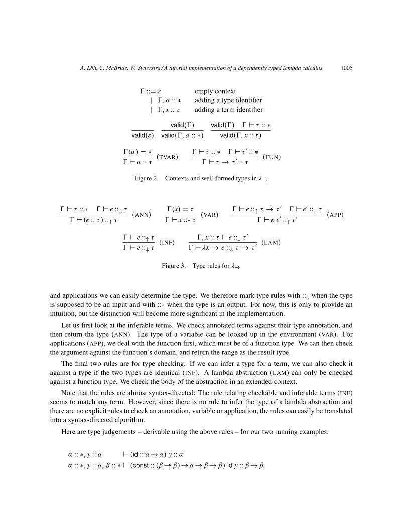
A. Loh, C. McBride, W. Swierstra / A tutorial implementation of a dependently typed lambda calculus 1005
0 ::= ε empty context| 0, α :: ∗ adding a type identifier| 0, x :: τ adding a term identifier
valid(ε)
valid(0)
valid(0, α :: ∗)valid(0) 0 ` τ :: ∗
valid(0, x :: τ)
0(α) = ∗
0 ` α :: ∗(TVAR)
0 ` τ :: ∗ 0 ` τ ′ :: ∗0 ` τ → τ ′ :: ∗
(FUN)
Figure 2. Contexts and well-formed types in λ→
0 ` τ :: ∗ 0 ` e ::↓ τ
0 ` (e :: τ) ::↑ τ(ANN)
0(x) = τ
0 ` x ::↑ τ(VAR)
0 ` e ::↑ τ → τ ′ 0 ` e′ ::↓ τ
0 ` e e′ ::↑ τ ′(APP)
0 ` e ::↑ τ
0 ` e ::↓ τ(INF)
0, x :: τ ` e ::↓ τ ′
0 ` λx→ e ::↓ τ → τ ′(LAM)
Figure 3. Type rules for λ→
and applications we can easily determine the type. We therefore mark type rules with ::↓ when the typeis supposed to be an input and with ::↑ when the type is an output. For now, this is only to provide anintuition, but the distinction will become more significant in the implementation.
Let us first look at the inferable terms. We check annotated terms against their type annotation, andthen return the type (ANN). The type of a variable can be looked up in the environment (VAR). Forapplications (APP), we deal with the function first, which must be of a function type. We can then checkthe argument against the function’s domain, and return the range as the result type.
The final two rules are for type checking. If we can infer a type for a term, we can also check itagainst a type if the two types are identical (INF). A lambda abstraction (LAM) can only be checkedagainst a function type. We check the body of the abstraction in an extended context.
Note that the rules are almost syntax-directed: The rule relating checkable and inferable terms (INF)seems to match any term. However, since there is no rule to infer the type of a lambda abstraction andthere are no explicit rules to check an annotation, variable or application, the rules can easily be translatedinto a syntax-directed algorithm.
Here are type judgements – derivable using the above rules – for our two running examples:
α :: ∗, y :: α ` (id :: α→α) y :: α
α :: ∗, y :: α, β :: ∗ ` (const :: (β→β)→α→β→β) id y :: β→β
1006 A. Loh, C. McBride, W. Swierstra / A tutorial implementation of a dependently typed lambda calculus
2.4. Implementation
We now give an implementation of λ→ in Haskell. We provide an evaluator for well-typed expressions,and functions to type-check λ→ terms. The implementation follows the formal description that we havejust introduced very closely.
There is a certain freedom in how to implement the rules. We pick an implementation that allowsus to follow the type system closely, and that reduces the amount of technical overhead to a relativeminimum, so that we can concentrate on the essence of the algorithms involved. In what follows, webriefly discuss our design decisions and mention alternatives. It is important to point out that none ofthese decisions is essential for implementing dependent types.
Representing bound variables There are different possibilities to represent bound variables – all ofthem have advantages, and in order to exploit a maximum of advantages, we choose different represen-tations in different places of our implementation.
We represent locally bound variables by de Bruijn indices: variable occurrences are represented bynumbers instead of strings or letters, the number indicating how many binders occur between its binderand the occurrence. For example, we can write id as λ → 0, and const as λ → λ → 1 using de Bruijnindices. The advantage of this representation is that variables never have to be renamed, i.e., α-equalityof terms reduces to syntactic equality of terms.
The disadvantage of using de Bruijn indices is that they cannot be used to represent terms with freevariables, and whenever we encounter a lambda while type checking, we have to check the body ofthe expression which then has free variables. We therefore represent such free variables in terms usingstrings. The combination of using numbers for variables local, and strings for variables global to thecurrent term is called a locally nameless representation [12].
Finally, we use higher-order abstract syntax to represent values: values that are functions are rep-resented using Haskell functions. This has the advantage that we can use Haskell’s function applicationand do not have to implement substitution ourselves, and need not worry about name capture. A slightdownside of this approach is that Haskell functions can neither be shown nor compared for equality. For-tunately, this drawback can easily be alleviated by quoting a value back into a concrete representation.We will return to quoting once we have defined the evaluator and the type checker.
Separating inferable and checkable terms As we have already hinted at in the presentation of thetype rules for λ→ in Figure 3, we choose to distinguish terms for which the type can be read off (calledinferable terms) and terms for which we need a type to check them.
This distinction has the advantage that we can give precise and total definitions of all the functionsinvolved in the type checker and evaluator. Another possibility is to require every lambda-abstractedvariable to be explicitly annotated in the abstract syntax – we would then have inferable terms exclusively.It is, however, very useful to be able to annotate any term. In the presence of general annotations, it is nolonger necessary to require an annotation on every lambda-bound variable. In fact, allowing un-annotatedlambdas gives us quite a bit of convenience without extra cost: applications of the form e (λx→ e′) canbe processed without type annotation, because the type of x is determined by the type of e.
A. Loh, C. McBride, W. Swierstra / A tutorial implementation of a dependently typed lambda calculus 1007
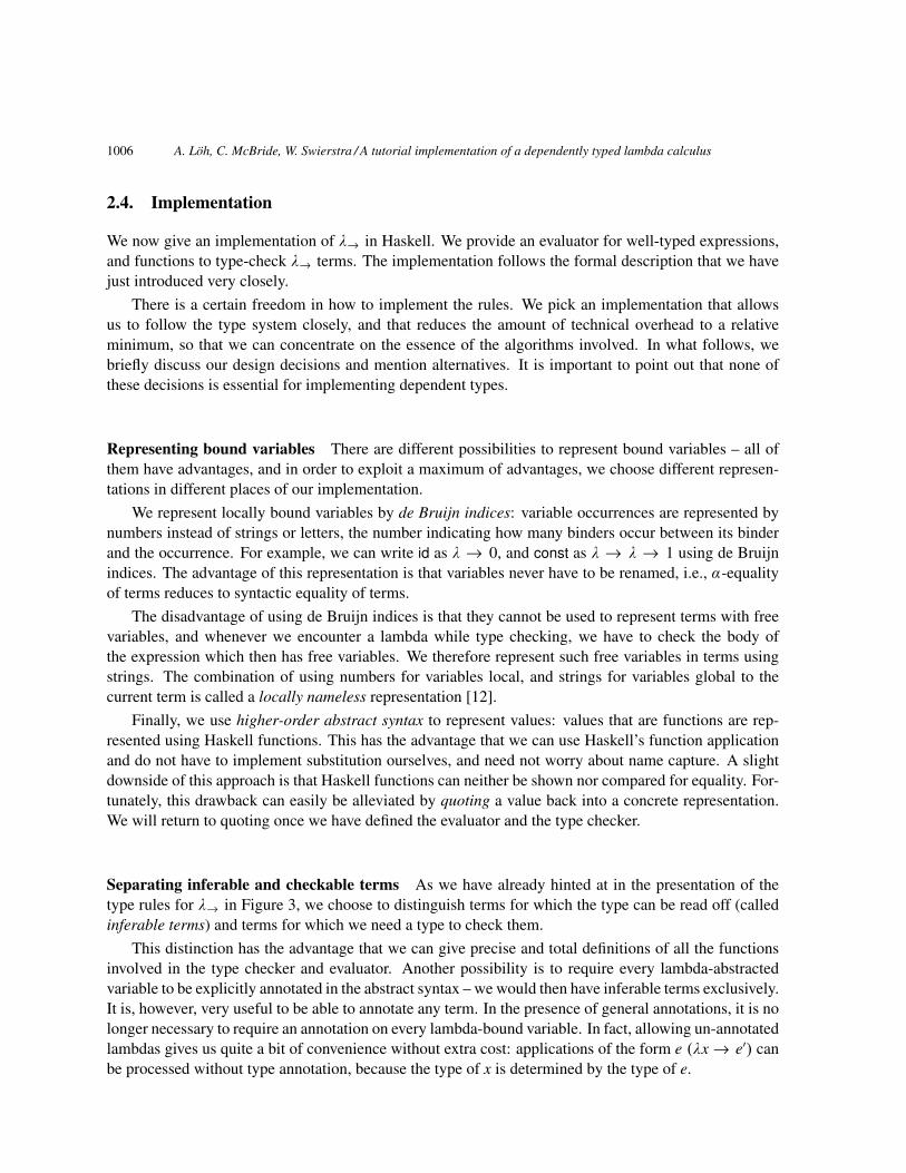
Abstract syntax We introduce data types for inferable (Term↑) and checkable (Term↓) terms, and fornames.
data Term↑= Ann Term↓ Type| Bound Int| Free Name| Term↑ :@: Term↓
deriving (Show, Eq)
data Term↓= Inf Term↑| Lam Term↓
deriving (Show, Eq)
data Name= Global String| Local Int| Quote Int
deriving (Show, Eq)
Annotated terms are represented using Ann. As explained above, we use integers to represent bound vari-ables (Bound), and names for free variables (Free). Names usually refer to global entities using strings.When passing a binder in an algorithm, we have to convert a bound variable into a free variable temporar-ily, and use Local for that. During quoting, we will use the Quote constructor. The infix constructor :@:denotes application.
Inferable terms are embedded in the checkable terms via the constructor Inf , and lambda abstractions(which do not introduce an explicit variable due to our use of de Bruijn indices) are written using Lam.
Types consist only of type identifiers (TFree) or function arrows (Fun). We reuse the Name data typefor type identifiers. In λ→, there are no bound names on the type level, so there is no need for a TBoundconstructor.
data Type= TFree Name| Fun Type Type
deriving (Show, Eq)
Values are lambda abstractions (VLam) or neutral terms (VNeutral).
data Value= VLam (Value→ Value)
| VNeutral Neutral
As described in the discussion on higher-order abstract syntax, we represent function values as Haskellfunctions of type Value → Value. For instance, the term const – when evaluated – results in the valueVLam (λx→ VLam (λy→ x)).
The data type for neutral terms matches the formal abstract syntax exactly. A neutral term is either avariable (NFree), or an application of a neutral term to a value (NApp).
1008 A. Loh, C. McBride, W. Swierstra / A tutorial implementation of a dependently typed lambda calculus
data Neutral= NFree Name| NApp Neutral Value
We introduce a function vfree that creates the value corresponding to a free variable:
vfree :: Name→ Valuevfree n = VNeutral (NFree n)
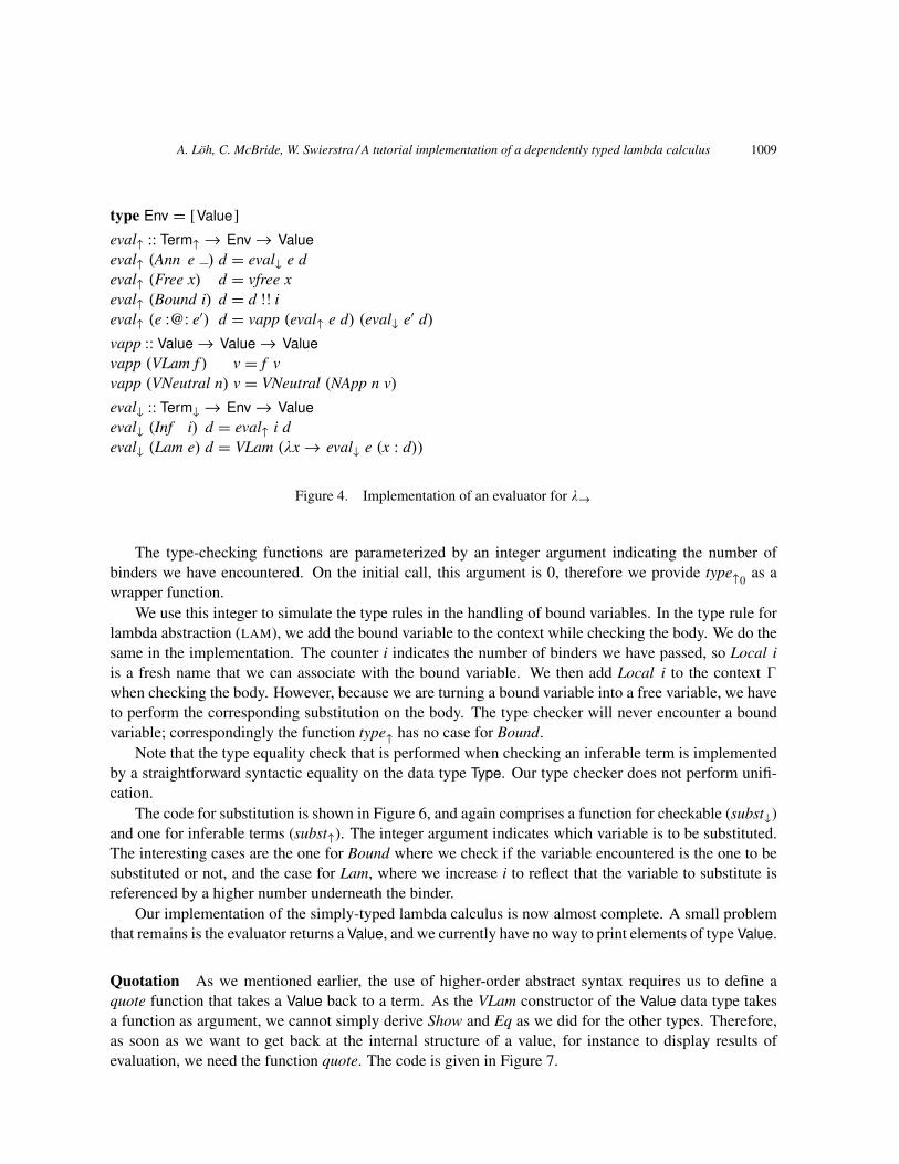
Evaluation The code for evaluation is given in Figure 4. The functions eval↑ and eval↓ implement thebig-step evaluation rules for inferable and checkable terms respectively. Comparing the code to the rulesin Figure 1 reveals that the implementation is mostly straightforward.
Substitution is handled by passing around an environment of values. Since bound variables arerepresented as integers, the environment is just a list of values where the i-th position corresponds to thevalue of variable i. We add a new element to the environment whenever evaluating underneath a binder,and lookup the correct element (using Haskell’s list lookup operator (!!)) when we encounter a boundvariable.
For lambda functions (Lam), we introduce a Haskell function and add the bound variable x to theenvironment while evaluating the body.
Contexts Before we can tackle the implementation of type checking, we have to define contexts. Con-texts are implemented as (reversed) lists associating names with either ∗ (HasKind Star) or a type(HasType t):
data Kind = Starderiving (Show)
data Info= HasKind Kind| HasType Type
deriving (Show)
type Context = [(Name, Info)]
Extending a context is thus achieved by the list “cons” operation; looking up a name in a context isperformed by the Haskell standard list function lookup.
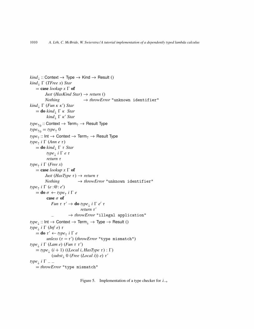
Type checking We now implement the rules in Figure 3. The code is shown in Figure 5. The typechecking algorithm can fail, and to do so gracefully, it returns a result in the Result monad. For simplicity,we choose a standard error monad in this presentation:
type Result α = Either String α
We use the function throwError :: String→ Result α to report an error.The function for inferable terms type↑ returns a type, whereas the function for checkable terms type↓
takes a type as input and returns (). The well-formedness of types is checked using the function kind↓.Each case of the definitions corresponds directly to one of the rules.
A. Loh, C. McBride, W. Swierstra / A tutorial implementation of a dependently typed lambda calculus 1009
type Env = [Value]eval↑ :: Term↑→ Env→ Valueeval↑ (Ann e ) d = eval↓ e deval↑ (Free x) d = vfree xeval↑ (Bound i) d = d !! ieval↑ (e :@: e′) d = vapp (eval↑ e d) (eval↓ e′ d)
vapp :: Value→ Value→ Valuevapp (VLam f ) v = f vvapp (VNeutral n) v = VNeutral (NApp n v)
eval↓ :: Term↓→ Env→ Valueeval↓ (Inf i) d = eval↑ i deval↓ (Lam e) d = VLam (λx→ eval↓ e (x : d))
Figure 4. Implementation of an evaluator for λ→
The type-checking functions are parameterized by an integer argument indicating the number ofbinders we have encountered. On the initial call, this argument is 0, therefore we provide type↑0 as awrapper function.
We use this integer to simulate the type rules in the handling of bound variables. In the type rule forlambda abstraction (LAM), we add the bound variable to the context while checking the body. We do thesame in the implementation. The counter i indicates the number of binders we have passed, so Local iis a fresh name that we can associate with the bound variable. We then add Local i to the context 0
when checking the body. However, because we are turning a bound variable into a free variable, we haveto perform the corresponding substitution on the body. The type checker will never encounter a boundvariable; correspondingly the function type↑ has no case for Bound.
Note that the type equality check that is performed when checking an inferable term is implementedby a straightforward syntactic equality on the data type Type. Our type checker does not perform unifi-cation.
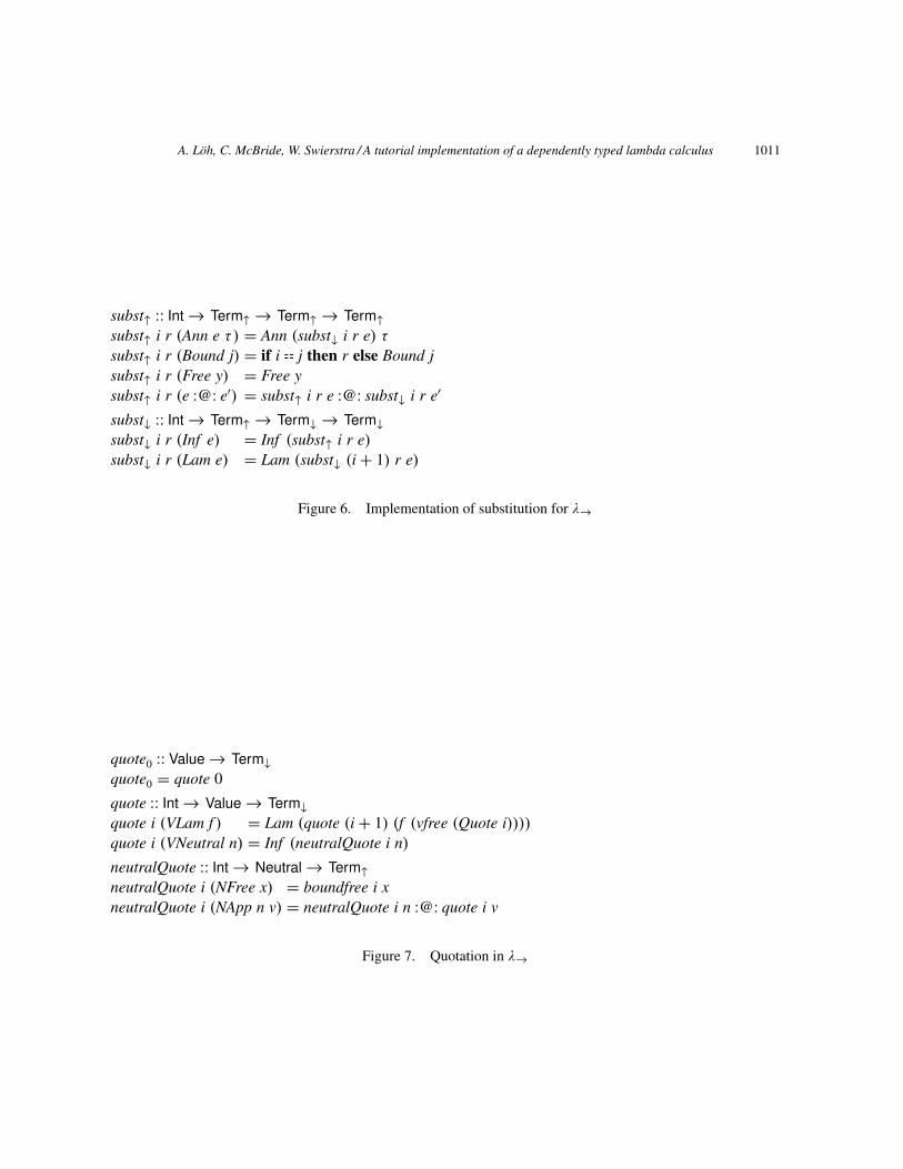
The code for substitution is shown in Figure 6, and again comprises a function for checkable (subst↓)and one for inferable terms (subst↑). The integer argument indicates which variable is to be substituted.The interesting cases are the one for Bound where we check if the variable encountered is the one to besubstituted or not, and the case for Lam, where we increase i to reflect that the variable to substitute isreferenced by a higher number underneath the binder.
Our implementation of the simply-typed lambda calculus is now almost complete. A small problemthat remains is the evaluator returns a Value, and we currently have no way to print elements of type Value.
Quotation As we mentioned earlier, the use of higher-order abstract syntax requires us to define aquote function that takes a Value back to a term. As the VLam constructor of the Value data type takesa function as argument, we cannot simply derive Show and Eq as we did for the other types. Therefore,as soon as we want to get back at the internal structure of a value, for instance to display results ofevaluation, we need the function quote. The code is given in Figure 7.
1010 A. Loh, C. McBride, W. Swierstra / A tutorial implementation of a dependently typed lambda calculus
kind↓ :: Context→ Type→ Kind→ Result ()
kind↓ 0 (TFree x) Star= case lookup x 0 of
Just (HasKind Star)→ return ()
Nothing → throwError "unknown identifier"kind↓ 0 (Fun κ κ ′) Star= do kind↓ 0 κ Star
kind↓ 0 κ ′ Star
type↑0 :: Context→ Term↑→ Result Typetype↑0 = type↑ 0type↑ :: Int→ Context→ Term↑→ Result Typetype↑ i 0 (Ann e τ)
= do kind↓ 0 τ Startype↓ i 0 e τ
return τ
type↑ i 0 (Free x)= case lookup x 0 of
Just (HasType τ)→ return τ
Nothing → throwError "unknown identifier"type↑ i 0 (e :@: e′)= do σ ← type↑ i 0 e
case σ ofFun τ τ ′→ do type↓ i 0 e′ τ
return τ ′
→ throwError "illegal application"
type↓ :: Int→ Context→ Term↓→ Type→ Result ()
type↓ i 0 (Inf e) τ
= do τ ′← type↑ i 0 eunless (τ = = τ ′) (throwError "type mismatch")
type↓ i 0 (Lam e) (Fun τ τ ′)
= type↓ (i+ 1) ((Local i, HasType τ) : 0)
(subst↓ 0 (Free (Local i)) e) τ ′
type↓ i 0
= throwError "type mismatch"
Figure 5. Implementation of a type checker for λ→
A. Loh, C. McBride, W. Swierstra / A tutorial implementation of a dependently typed lambda calculus 1011
subst↑ :: Int→ Term↑→ Term↑→ Term↑subst↑ i r (Ann e τ) = Ann (subst↓ i r e) τ
subst↑ i r (Bound j) = if i = = j then r else Bound jsubst↑ i r (Free y) = Free ysubst↑ i r (e :@: e′) = subst↑ i r e :@: subst↓ i r e′
subst↓ :: Int→ Term↑→ Term↓→ Term↓subst↓ i r (Inf e) = Inf (subst↑ i r e)subst↓ i r (Lam e) = Lam (subst↓ (i+ 1) r e)
Figure 6. Implementation of substitution for λ→
quote0 :: Value→ Term↓quote0 = quote 0quote :: Int→ Value→ Term↓quote i (VLam f ) = Lam (quote (i+ 1) (f (vfree (Quote i))))quote i (VNeutral n) = Inf (neutralQuote i n)
neutralQuote :: Int→ Neutral→ Term↑neutralQuote i (NFree x) = boundfree i xneutralQuote i (NApp n v) = neutralQuote i n :@: quote i v
Figure 7. Quotation in λ→
1012 A. Loh, C. McBride, W. Swierstra / A tutorial implementation of a dependently typed lambda calculus
The function quote takes an integer argument that counts the number of binders we have traversed.Initially, quote is always called with 0, so we wrap this call in the function quote0.
If the value is a lambda abstraction, we generate a fresh variable Quote i and apply the Haskellfunction f to this fresh variable. The value resulting from the function application is then quoted atlevel i+ 1. We use the constructor Quote that takes an argument of type Int here to ensure that the newlycreated names do not clash with other names in the value.
If the value is a neutral term (hence an application of a free variable to other values), the functionneutralQuote is used to quote the arguments. The boundfree function checks if the variable occurring atthe head of the application is a Quote and thus a bound variable, or a free name:
boundfree :: Int→ Name→ Term↑boundfree i (Quote k) = Bound (i− k − 1)
boundfree i x = Free x
Quotation of functions is best understood by example. The value corresponding to the term const isVLam (λx→ VLam (λy→ x)). Applying quote0 yields the following:
quote 0 (VLam (λx→ VLam (λy→ x)))= Lam (quote 1 (VLam (λy→ vfree (Quote 0))))
= Lam (Lam (quote 2 (vfree (Quote 0))))
= Lam (Lam (neutralQuote 2 (NFree (Quote 0))))
= Lam (Lam (Bound 1))
When quote moves underneath a binder, we introduce a temporary name for the bound variable. Toensure that names invented during quotation do not interfere with any other names, we only use theconstructor Quote during the quotation process. If the bound variable actually occurs in the body ofthe function, we will sooner or later arrive at those occurrences. We can then generate the correct deBruijn index by determining the number of binders we have passed between introducing and observingthe Quote variable.
Examples We can now test the implementation on our running examples. We make the followingdefinitions
id′ = Lam (Inf (Bound 0))
const′ = Lam (Lam (Inf (Bound 1)))
tfree α = TFree (Global α)
free x = Inf (Free (Global x))
term1 = Ann id′ (Fun (tfree "a") (tfree "a")) :@: free "y"term2 = Ann const′ (Fun (Fun (tfree "b") (tfree "b"))
(Fun (tfree "a")(Fun (tfree "b") (tfree "b"))))
:@: id′ :@: free "y"
env1 = [(Global "y", HasType (tfree "a")),(Global "a", HasKind Star)]
env2 = [(Global "b", HasKind Star)]++ env1
A. Loh, C. McBride, W. Swierstra / A tutorial implementation of a dependently typed lambda calculus 1013
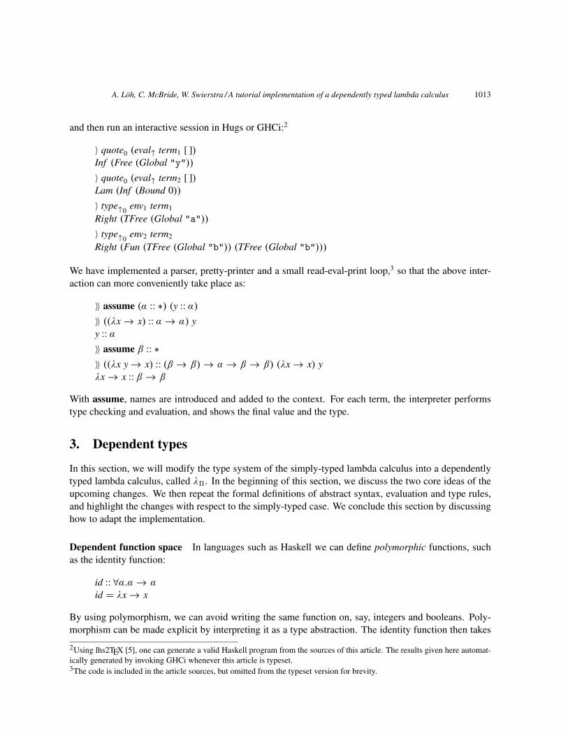
and then run an interactive session in Hugs or GHCi:2
〉 quote0 (eval↑ term1 [ ])Inf (Free (Global "y"))
〉 quote0 (eval↑ term2 [ ])Lam (Inf (Bound 0))
〉 type↑0 env1 term1
Right (TFree (Global "a"))
〉 type↑0 env2 term2
Right (Fun (TFree (Global "b")) (TFree (Global "b")))
We have implemented a parser, pretty-printer and a small read-eval-print loop,3 so that the above inter-action can more conveniently take place as:
〉〉 assume (α :: ∗) (y :: α)
〉〉 ((λx→ x) :: α→ α) yy :: α
〉〉 assume β :: ∗〉〉 ((λx y→ x) :: (β → β)→ α→ β → β) (λx→ x) yλx→ x :: β → β
With assume, names are introduced and added to the context. For each term, the interpreter performstype checking and evaluation, and shows the final value and the type.
3. Dependent types
In this section, we will modify the type system of the simply-typed lambda calculus into a dependentlytyped lambda calculus, called λ5. In the beginning of this section, we discuss the two core ideas of theupcoming changes. We then repeat the formal definitions of abstract syntax, evaluation and type rules,and highlight the changes with respect to the simply-typed case. We conclude this section by discussinghow to adapt the implementation.
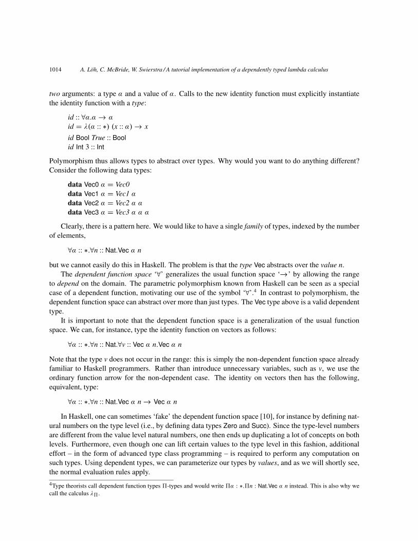
Dependent function space In languages such as Haskell we can define polymorphic functions, suchas the identity function:
id :: ∀α.α→ α
id = λx→ x
By using polymorphism, we can avoid writing the same function on, say, integers and booleans. Poly-morphism can be made explicit by interpreting it as a type abstraction. The identity function then takes
2Using lhs2TEX [5], one can generate a valid Haskell program from the sources of this article. The results given here automat-ically generated by invoking GHCi whenever this article is typeset.3The code is included in the article sources, but omitted from the typeset version for brevity.
1014 A. Loh, C. McBride, W. Swierstra / A tutorial implementation of a dependently typed lambda calculus
two arguments: a type α and a value of α. Calls to the new identity function must explicitly instantiatethe identity function with a type:
id :: ∀α.α→ α
id = λ(α :: ∗) (x :: α)→ x
id Bool True :: Boolid Int 3 :: Int
Polymorphism thus allows types to abstract over types. Why would you want to do anything different?Consider the following data types:
data Vec0 α = Vec0data Vec1 α = Vec1 α
data Vec2 α = Vec2 α α
data Vec3 α = Vec3 α α α
Clearly, there is a pattern here. We would like to have a single family of types, indexed by the numberof elements,
∀α :: ∗.∀n :: Nat.Vec α n
but we cannot easily do this in Haskell. The problem is that the type Vec abstracts over the value n.The dependent function space ‘∀’ generalizes the usual function space ‘→’ by allowing the range
to depend on the domain. The parametric polymorphism known from Haskell can be seen as a specialcase of a dependent function, motivating our use of the symbol ‘∀’.4 In contrast to polymorphism, thedependent function space can abstract over more than just types. The Vec type above is a valid dependenttype.
It is important to note that the dependent function space is a generalization of the usual functionspace. We can, for instance, type the identity function on vectors as follows:
∀α :: ∗.∀n :: Nat.∀v :: Vec α n.Vec α n
Note that the type v does not occur in the range: this is simply the non-dependent function space alreadyfamiliar to Haskell programmers. Rather than introduce unnecessary variables, such as v, we use theordinary function arrow for the non-dependent case. The identity on vectors then has the following,equivalent, type:
∀α :: ∗.∀n :: Nat.Vec α n→ Vec α n
In Haskell, one can sometimes ‘fake’ the dependent function space [10], for instance by defining nat-ural numbers on the type level (i.e., by defining data types Zero and Succ). Since the type-level numbersare different from the value level natural numbers, one then ends up duplicating a lot of concepts on bothlevels. Furthermore, even though one can lift certain values to the type level in this fashion, additionaleffort – in the form of advanced type class programming – is required to perform any computation onsuch types. Using dependent types, we can parameterize our types by values, and as we will shortly see,the normal evaluation rules apply.
4Type theorists call dependent function types 5-types and would write 5α : ∗.5n : Nat.Vec α n instead. This is also why wecall the calculus λ5.
A. Loh, C. McBride, W. Swierstra / A tutorial implementation of a dependently typed lambda calculus 1015
e ⇓ ve :: ρ ⇓ v ∗ ⇓ ∗
ρ ⇓ τ ρ ′ ⇓ τ ′
∀x :: ρ.ρ ′ ⇓ ∀x :: τ.τ ′ x ⇓ x
e ⇓ λx→ v e′ ⇓ v′
e e′ ⇓ v[x 7→ v′ ]e ⇓ n e′ ⇓ v′
e e′ ⇓ n v′e ⇓ v
λx→ e ⇓ λx→ v
Figure 8. Evaluation in λ5
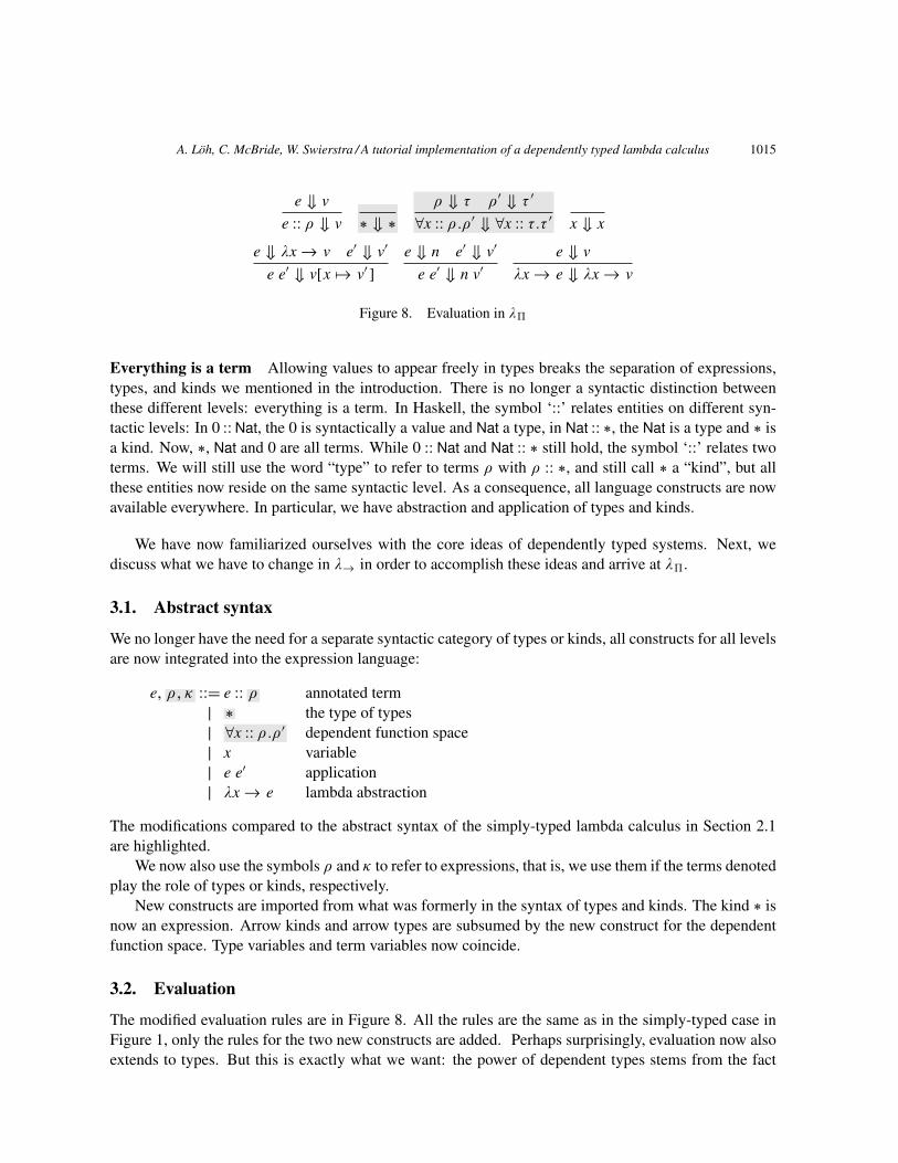
Everything is a term Allowing values to appear freely in types breaks the separation of expressions,types, and kinds we mentioned in the introduction. There is no longer a syntactic distinction betweenthese different levels: everything is a term. In Haskell, the symbol ‘::’ relates entities on different syn-tactic levels: In 0 :: Nat, the 0 is syntactically a value and Nat a type, in Nat :: ∗, the Nat is a type and ∗ isa kind. Now, ∗, Nat and 0 are all terms. While 0 :: Nat and Nat :: ∗ still hold, the symbol ‘::’ relates twoterms. We will still use the word “type” to refer to terms ρ with ρ :: ∗, and still call ∗ a “kind”, but allthese entities now reside on the same syntactic level. As a consequence, all language constructs are nowavailable everywhere. In particular, we have abstraction and application of types and kinds.
We have now familiarized ourselves with the core ideas of dependently typed systems. Next, wediscuss what we have to change in λ→ in order to accomplish these ideas and arrive at λ5.
3.1. Abstract syntax
We no longer have the need for a separate syntactic category of types or kinds, all constructs for all levelsare now integrated into the expression language:
e, ρ, κ ::= e :: ρ annotated term| ∗ the type of types| ∀x :: ρ.ρ ′ dependent function space| x variable| e e′ application| λx→ e lambda abstraction
The modifications compared to the abstract syntax of the simply-typed lambda calculus in Section 2.1are highlighted.
We now also use the symbols ρ and κ to refer to expressions, that is, we use them if the terms denotedplay the role of types or kinds, respectively.
New constructs are imported from what was formerly in the syntax of types and kinds. The kind ∗ isnow an expression. Arrow kinds and arrow types are subsumed by the new construct for the dependentfunction space. Type variables and term variables now coincide.
3.2. Evaluation
The modified evaluation rules are in Figure 8. All the rules are the same as in the simply-typed case inFigure 1, only the rules for the two new constructs are added. Perhaps surprisingly, evaluation now alsoextends to types. But this is exactly what we want: the power of dependent types stems from the fact
1016 A. Loh, C. McBride, W. Swierstra / A tutorial implementation of a dependently typed lambda calculus
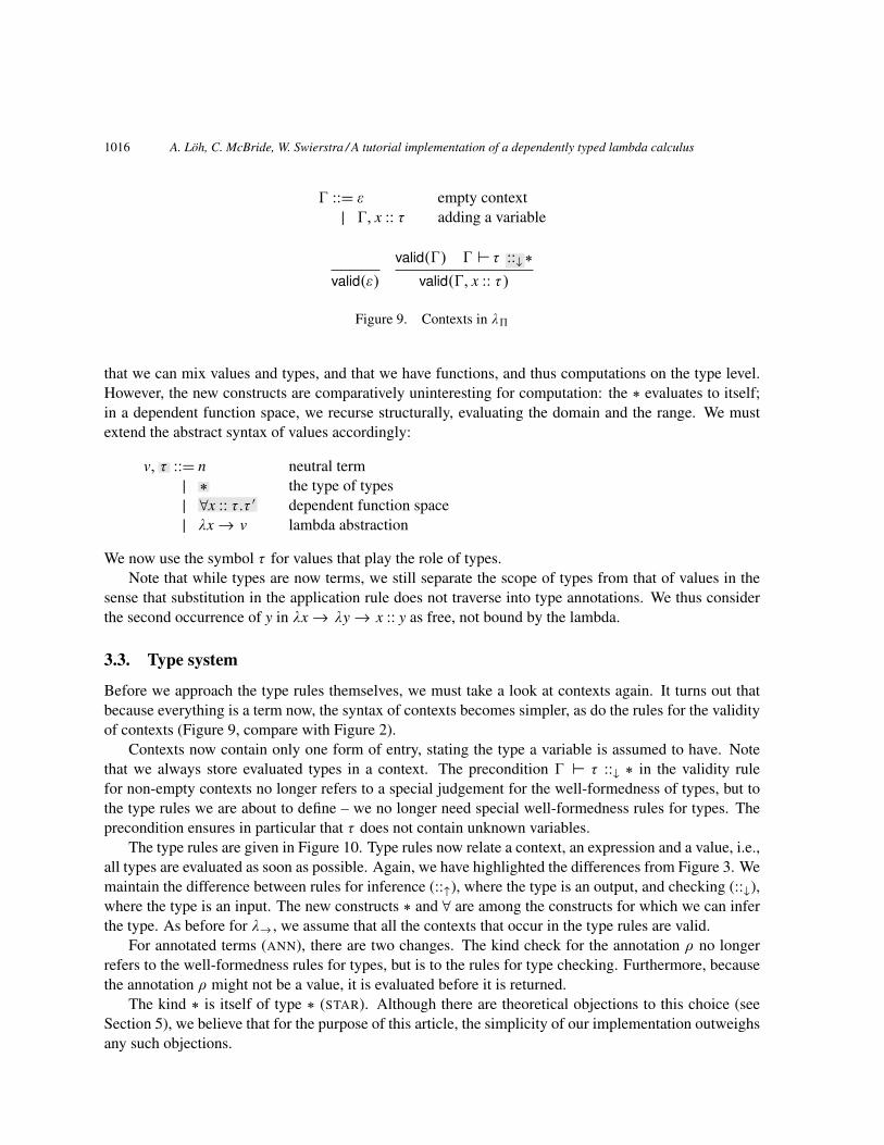
0 ::= ε empty context| 0, x :: τ adding a variable
valid(ε)
valid(0) 0 ` τ ::↓∗valid(0, x :: τ)
Figure 9. Contexts in λ5
that we can mix values and types, and that we have functions, and thus computations on the type level.However, the new constructs are comparatively uninteresting for computation: the ∗ evaluates to itself;in a dependent function space, we recurse structurally, evaluating the domain and the range. We mustextend the abstract syntax of values accordingly:
v, τ ::= n neutral term| ∗ the type of types| ∀x :: τ.τ ′ dependent function space| λx→ v lambda abstraction
We now use the symbol τ for values that play the role of types.Note that while types are now terms, we still separate the scope of types from that of values in the
sense that substitution in the application rule does not traverse into type annotations. We thus considerthe second occurrence of y in λx→ λy→ x :: y as free, not bound by the lambda.
3.3. Type system
Before we approach the type rules themselves, we must take a look at contexts again. It turns out thatbecause everything is a term now, the syntax of contexts becomes simpler, as do the rules for the validityof contexts (Figure 9, compare with Figure 2).
Contexts now contain only one form of entry, stating the type a variable is assumed to have. Notethat we always store evaluated types in a context. The precondition 0 ` τ ::↓ ∗ in the validity rulefor non-empty contexts no longer refers to a special judgement for the well-formedness of types, but tothe type rules we are about to define – we no longer need special well-formedness rules for types. Theprecondition ensures in particular that τ does not contain unknown variables.
The type rules are given in Figure 10. Type rules now relate a context, an expression and a value, i.e.,all types are evaluated as soon as possible. Again, we have highlighted the differences from Figure 3. Wemaintain the difference between rules for inference (::↑), where the type is an output, and checking (::↓),where the type is an input. The new constructs ∗ and ∀ are among the constructs for which we can inferthe type. As before for λ→, we assume that all the contexts that occur in the type rules are valid.
For annotated terms (ANN), there are two changes. The kind check for the annotation ρ no longerrefers to the well-formedness rules for types, but is to the rules for type checking. Furthermore, becausethe annotation ρ might not be a value, it is evaluated before it is returned.
The kind ∗ is itself of type ∗ (STAR). Although there are theoretical objections to this choice (seeSection 5), we believe that for the purpose of this article, the simplicity of our implementation outweighsany such objections.
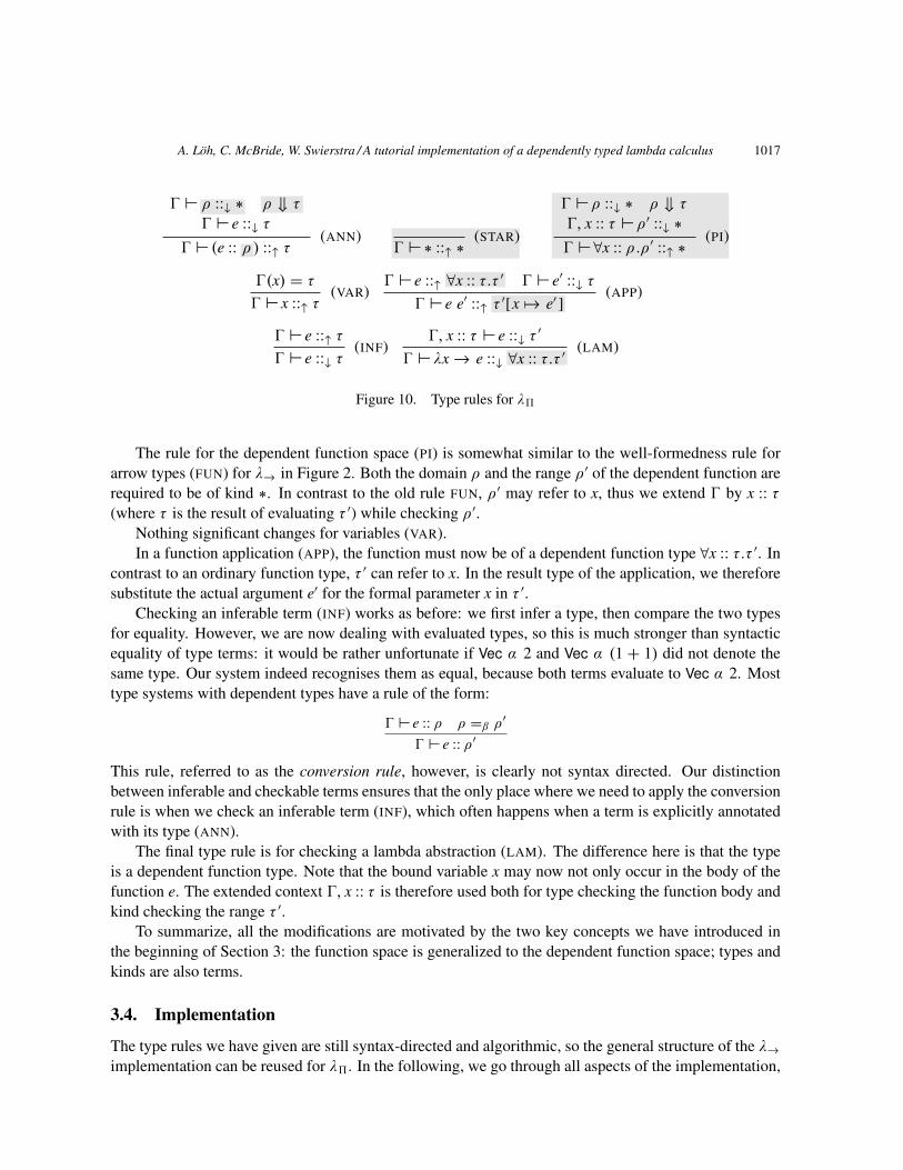
A. Loh, C. McBride, W. Swierstra / A tutorial implementation of a dependently typed lambda calculus 1017
0 ` ρ ::↓ ∗ ρ ⇓ τ
0 ` e ::↓ τ
0 ` (e :: ρ ) ::↑ τ(ANN)
0 ` ∗ ::↑ ∗(STAR)
0 ` ρ ::↓ ∗ ρ ⇓ τ
0, x :: τ ` ρ ′ ::↓ ∗0 ` ∀x :: ρ.ρ ′ ::↑ ∗
(PI)
0(x) = τ
0 ` x ::↑ τ(VAR)
0 ` e ::↑ ∀x :: τ.τ ′ 0 ` e′ ::↓ τ
0 ` e e′ ::↑ τ ′[x 7→ e′ ](APP)
0 ` e ::↑ τ
0 ` e ::↓ τ(INF)
0, x :: τ ` e ::↓ τ ′
0 ` λx→ e ::↓ ∀x :: τ.τ ′(LAM)
Figure 10. Type rules for λ5
The rule for the dependent function space (PI) is somewhat similar to the well-formedness rule forarrow types (FUN) for λ→ in Figure 2. Both the domain ρ and the range ρ ′ of the dependent function arerequired to be of kind ∗. In contrast to the old rule FUN, ρ ′ may refer to x, thus we extend 0 by x :: τ
(where τ is the result of evaluating τ ′) while checking ρ ′.Nothing significant changes for variables (VAR).In a function application (APP), the function must now be of a dependent function type ∀x :: τ.τ ′. In
contrast to an ordinary function type, τ ′ can refer to x. In the result type of the application, we thereforesubstitute the actual argument e′ for the formal parameter x in τ ′.
Checking an inferable term (INF) works as before: we first infer a type, then compare the two typesfor equality. However, we are now dealing with evaluated types, so this is much stronger than syntacticequality of type terms: it would be rather unfortunate if Vec α 2 and Vec α (1 + 1) did not denote thesame type. Our system indeed recognises them as equal, because both terms evaluate to Vec α 2. Mosttype systems with dependent types have a rule of the form:
0 ` e :: ρ ρ =β ρ′
0 ` e :: ρ′
This rule, referred to as the conversion rule, however, is clearly not syntax directed. Our distinctionbetween inferable and checkable terms ensures that the only place where we need to apply the conversionrule is when we check an inferable term (INF), which often happens when a term is explicitly annotatedwith its type (ANN).
The final type rule is for checking a lambda abstraction (LAM). The difference here is that the typeis a dependent function type. Note that the bound variable x may now not only occur in the body of thefunction e. The extended context 0, x :: τ is therefore used both for type checking the function body andkind checking the range τ ′.
To summarize, all the modifications are motivated by the two key concepts we have introduced inthe beginning of Section 3: the function space is generalized to the dependent function space; types andkinds are also terms.
3.4. Implementation
The type rules we have given are still syntax-directed and algorithmic, so the general structure of the λ→implementation can be reused for λ5. In the following, we go through all aspects of the implementation,
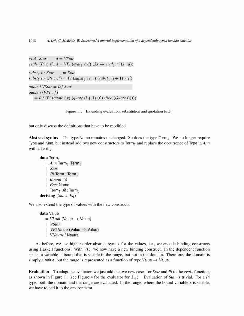
1018 A. Loh, C. McBride, W. Swierstra / A tutorial implementation of a dependently typed lambda calculus
eval↑ Star d = VStareval↑ (Pi τ τ ′) d = VPi (eval↓ τ d) (λx→ eval↓ τ ′ (x : d))
subst↑ i r Star = Starsubst↑ i r (Pi τ τ ′) = Pi (subst↓ i r τ) (subst↓ (i+ 1) r τ ′)
quote i VStar = Inf Starquote i (VPi v f )= Inf (Pi (quote i v) (quote (i+ 1) (f (vfree (Quote i)))))
Figure 11. Extending evaluation, substitution and quotation to λ5
but only discuss the definitions that have to be modified.
Abstract syntax The type Name remains unchanged. So does the type Term↓. We no longer requireType and Kind, but instead add two new constructors to Term↑ and replace the occurrence of Type in Annwith a Term↓:
data Term↑= Ann Term↓ Term↓| Star| Pi Term↓ Term↓| Bound Int| Free Name| Term↑ :@: Term↓
deriving (Show, Eq)
We also extend the type of values with the new constructs.
data Value= VLam (Value→ Value)
| VStar| VPi Value (Value→ Value)
| VNeutral Neutral
As before, we use higher-order abstract syntax for the values, i.e., we encode binding constructsusing Haskell functions. With VPi, we now have a new binding construct. In the dependent functionspace, a variable is bound that is visible in the range, but not in the domain. Therefore, the domain issimply a Value, but the range is represented as a function of type Value→ Value.
Evaluation To adapt the evaluator, we just add the two new cases for Star and Pi to the eval↑ function,as shown in Figure 11 (see Figure 4 for the evaluator for λ→). Evaluation of Star is trivial. For a Pitype, both the domain and the range are evaluated. In the range, where the bound variable x is visible,we have to add it to the environment.
A. Loh, C. McBride, W. Swierstra / A tutorial implementation of a dependently typed lambda calculus 1019
Contexts Contexts map variables to their types. Types are on the term level now. We store types intheir evaluated form, and thus define:
type Type = Valuetype Context = [(Name, Type)]
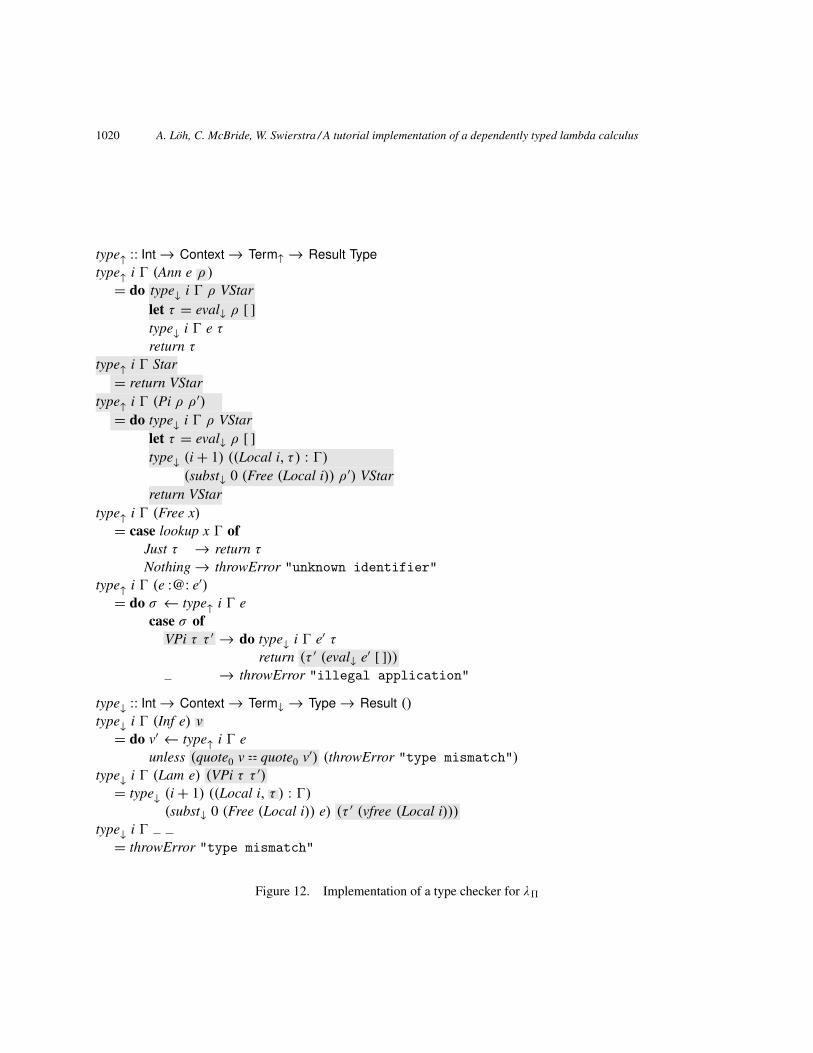
Type checking Let us go through each of the cases in Figure 12 one by one – for comparison, thecases for λ→are in Figure 5. For an annotated term, we first check that the annotation is a type of kind ∗,using the type-checking function type↓. We then evaluate the type. The resulting value τ is used to checkthe term e. If that succeeds, the entire expression has type v. Note that we assume that the term underconsideration in type↑ has no unbound variables, so all calls to eval↓ take an empty environment.
The (evaluated) type of Star is VStar.For a dependent function type, we first kind-check the domain τ . Then the domain is evaluated to v.
The value is added to the context while kind-checking the range, as also shown in the corresponding typerule PI.
There are no significant changes in the Free case.In the application case, the type inferred for the function is a Value now. This type must be of the form
VPi τ τ ′, i.e., a dependent function type. In the corresponding type rule in Figure 10, the bound variablex is substituted by e′ in the result type τ ′. In the implementation, τ ′ is a function, and the substitution isperformed by applying it to the (evaluated) e′.
In the case for Inf, we have to perform the type equality check. In contrast to the type rule INF, wecannot compare values for equality directly in Haskell. Instead, we quote them and compare the resultingterms syntactically.
In the case for Lam, we require a dependent function type of form VPi τ τ ′ now. As in the corre-sponding case for λ→, we add the bound variable (of type τ ) to the context while checking the body.But we now perform substitution on the function body e (using subst↓) and on the result type τ ′ (byapplying τ ′).
We thus only have to extend the substitution functions, by adding the usual two cases for Star and Pias shown in Figure 11. There’s nothing to subsitute for Star. For Pi, we have to increment the counterbefore substituting in the range because we pass a binder.
Quotation To complete our implementation of λ5, we only have to extend the quotation function. Thisoperation is more important than for λ→, because as we have seen, it is used in the equality check duringtype checking. Again, we only have to add equations for VStar and VPi, which are shown in Figure 11.
Quoting VStar yields Star. Since the dependent function type is a binding construct, quotation forVPi works similar to quotation of VLam: to quote the range, we increment the counter i, and apply theHaskell function representing the range to Quote i.
3.5. Where are the dependent types?
We now have adapted our type system and its implementation to dependent types, but unfortunately, wehave not yet seen any examples.
1020 A. Loh, C. McBride, W. Swierstra / A tutorial implementation of a dependently typed lambda calculus
type↑ :: Int→ Context→ Term↑→ Result Typetype↑ i 0 (Ann e ρ )
= do type↓ i 0 ρ VStarlet τ = eval↓ ρ [ ]type↓ i 0 e τ
return τ
type↑ i 0 Star= return VStar
type↑ i 0 (Pi ρ ρ ′)
= do type↓ i 0 ρ VStarlet τ = eval↓ ρ [ ]type↓ (i+ 1) ((Local i, τ ) : 0)
(subst↓ 0 (Free (Local i)) ρ ′) VStarreturn VStar
type↑ i 0 (Free x)= case lookup x 0 of
Just τ → return τ
Nothing→ throwError "unknown identifier"type↑ i 0 (e :@: e′)= do σ ← type↑ i 0 e
case σ ofVPi τ τ ′ → do type↓ i 0 e′ τ
return (τ ′ (eval↓ e′ [ ]))→ throwError "illegal application"
type↓ :: Int→ Context→ Term↓→ Type→ Result ()
type↓ i 0 (Inf e) v= do v′← type↑ i 0 e
unless (quote0 v = = quote0 v′) (throwError "type mismatch")type↓ i 0 (Lam e) (VPi τ τ ′)
= type↓ (i+ 1) ((Local i, τ ) : 0)
(subst↓ 0 (Free (Local i)) e) (τ ′ (vfree (Local i)))type↓ i 0
= throwError "type mismatch"
Figure 12. Implementation of a type checker for λ5
A. Loh, C. McBride, W. Swierstra / A tutorial implementation of a dependently typed lambda calculus 1021
Again, we have written a small interpreter around the type checker we have just presented, and wecan use it to define and check, for instance, the polymorphic identity function (where the type argumentis explicit), as follows:
〉〉 let id = (λα x→ x) :: ∀(α :: ∗).α→ α
id :: ∀(x :: ∗) (y :: x).x〉〉 assume (Bool :: ∗) (False :: Bool)
〉〉 id Boolλx→ x :: ∀x :: Bool.Bool〉〉 id Bool FalseFalse :: Bool
This is more than we can do in the simply-typed setting, but it is by no means spectacular and does notrequire dependent types. Unfortunately, while we have a framework for dependent types in place, wecannot write any interesting programs as long as we do not add at least a few specific data types to ourlanguage.
4. Beyond λ5
In Haskell, data types are introduced by special data declarations:
data Nat = Zero | Succ Nat
This introduces a new type Nat, together with two constructors Zero and Succ. In this section, weinvestigate how to extend our language with data types, such as natural numbers.
Obviously, we will need to add the type Nat together with its constructors; but how should we definefunctions, such as addition, that manipulate numbers? In Haskell, we would define a function that patternmatches on its arguments and makes recursive calls to smaller numbers:
plus :: Nat→ Nat→ Natplus Zero n = nplus (Succ k) n = Succ (plus k n)
In our calculus so far, we can neither pattern match nor make recursive calls. How could we hope todefine plus?
In Haskell, we can define recursive functions on data types using a fold [15]. Rather than introducepattern matching and recursion, and all the associated problems, we define functions over natural num-bers using the corresponding fold. In a dependently type setting, however, we can define a slightly moregeneral version of a fold called the eliminator.
The fold for natural numbers has the following type:
foldNat :: ∀α :: ∗.α→ (α→ α)→ Nat→ α
This much should be familiar. In the context of dependent types, however, there is no need for the typeα to be uniform across the constructors for natural numbers: rather than use α :: ∗, we use m :: Nat→ ∗.This leads us to the following type of natElim:
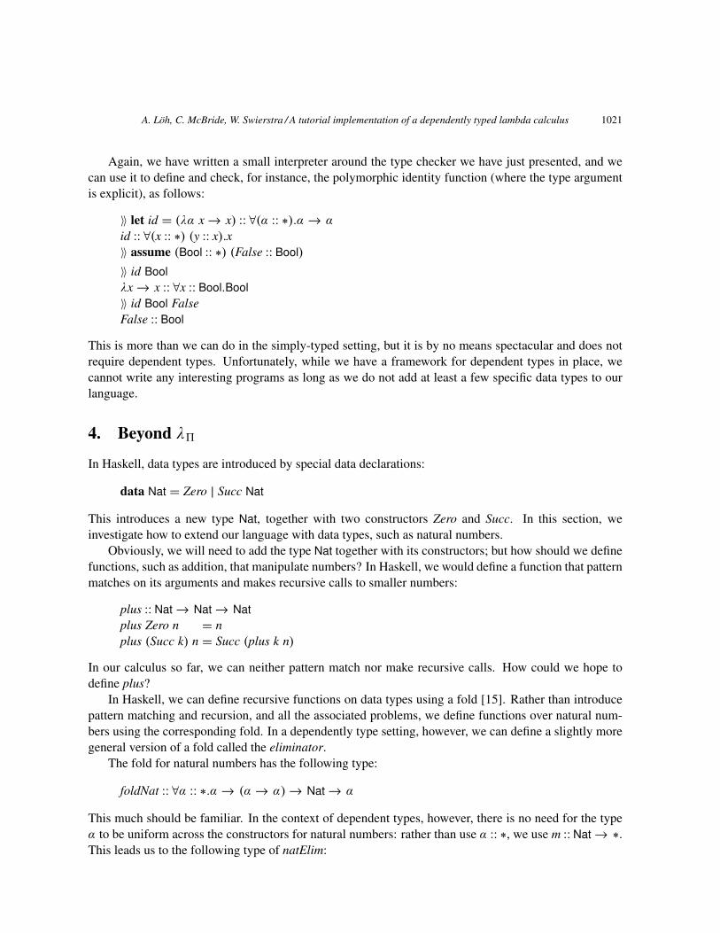
1022 A. Loh, C. McBride, W. Swierstra / A tutorial implementation of a dependently typed lambda calculus
Nat ⇓ Nat Zero ⇓ Zerok ⇓ l
Succ k ⇓ Succ l
mz ⇓ vnatElim m mz ms Zero ⇓ v
ms k (natElim m mz ms k) ⇓ vnatElim m mz ms (Succ k) ⇓ v
Figure 13. Evaluation of natural numbers
0 ` Nat :: ∗ 0 ` Zero :: Nat
0 ` k :: Nat
0 ` Succ k :: Nat
0 ` m :: Nat→ ∗0, m :: Nat→ ∗ ` mz :: m Zero
0, m :: Nat→ ∗ ` ms :: ∀k :: Nat.m k→ m (Succ k)0 ` n :: Nat
0 ` natElim m mz ms n :: m n
Figure 14. Typing rules for natural numbers
natElim :: ∀m :: Nat→ ∗. m Zero→ (∀k :: Nat.m k→ m (Succ k))→ ∀n :: Nat.m n
The first argument of the eliminator is the sometimes referred to as the motive [9]; it explains the reasonwe want to eliminate natural numbers. The second argument corresponds to the base case, where n isZero; the third argument corresponds to the inductive case where n is Succ k, for some k. In the inductivecase, we must describe how to construct m (Succ k) from k and m k. The result of natElim is a functionthat given any natural number n, will compute a value of type m n.
In summary, adding natural numbers to our language involves adding three separate elements: thetype Nat, the constructors Zero and Succ, and the eliminator natElim.
4.1. Implementing natural numbers
To implement these three components, we extend the abstract syntax and correspondingly add new casesto the evaluation and type checking functions. These new cases do not require any changes to existingcode; we choose to focus only on the new code fragments.
Abstract Syntax To implement natural numbers, we extend our abstract syntax as follows:
data Term↑ = . . .
| Nat| NatElim Term↓ Term↓ Term↓ Term↓
data Term↓ = . . .
| Zero| Succ Term↓
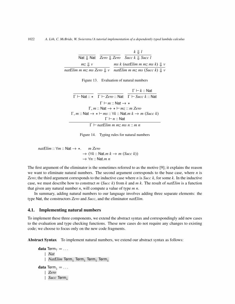
A. Loh, C. McBride, W. Swierstra / A tutorial implementation of a dependently typed lambda calculus 1023
eval↓ Zero d = VZeroeval↓ (Succ k) d = VSucc (eval↓ k d)
eval↑ Nat d = VNateval↑ (NatElim m mz ms n) d= let mzVal = eval↓ mz d
msVal = eval↓ ms drec nVal =
case nVal ofVZero → mzValVSucc k → msVal ‘vapp‘ k ‘vapp‘ rec kVNeutral n→ VNeutral
(NNatElim (eval↓ m d) mzVal msVal n)
→ error "internal: eval natElim"in rec (eval↓ n d)
Figure 15. Extending the evaluator natural numbers
We add new constructors corresponding to the type of and eliminator for natural numbers to theTerm↑ data type. The NatElim constructor is fully applied: it expects no further arguments.
Similarly, we extend Term↓ with the constructors for natural numbers. This may seem odd: we willalways know the type of Zero and Succ, so why not add them to Term↑ instead? For more complicatedtypes, however, such as dependent pairs, it is not always possible to infer the type of the constructorwithout a type annotation. We choose to add all constructors to Term↓, as this scheme will work for alldata types.
Evaluation We need to rethink our data type for values. Previously, values consisted exclusively oflambda abstractions and ‘stuck’ applications. Clearly, we will need to extend the data type for values tocope with the new constructors for natural numbers.
data Value = . . .
| VNat| VZero| VSucc Value
Introducing the eliminator, however, also complicates evaluation. The eliminator for natural numberscan also be stuck when the number being eliminated does not evaluate to a constructor. Correspondingly,we extend the data type for neutral terms to cover this case:
data Neutral = . . .
| NNatElim Value Value Value Neutral
The implementation of evaluation in Figure 15 closely follows the rules in Figure 13. The elimi-nator is the only interesting case. Essentially, the eliminator evaluates to the Haskell function with the
1024 A. Loh, C. McBride, W. Swierstra / A tutorial implementation of a dependently typed lambda calculus
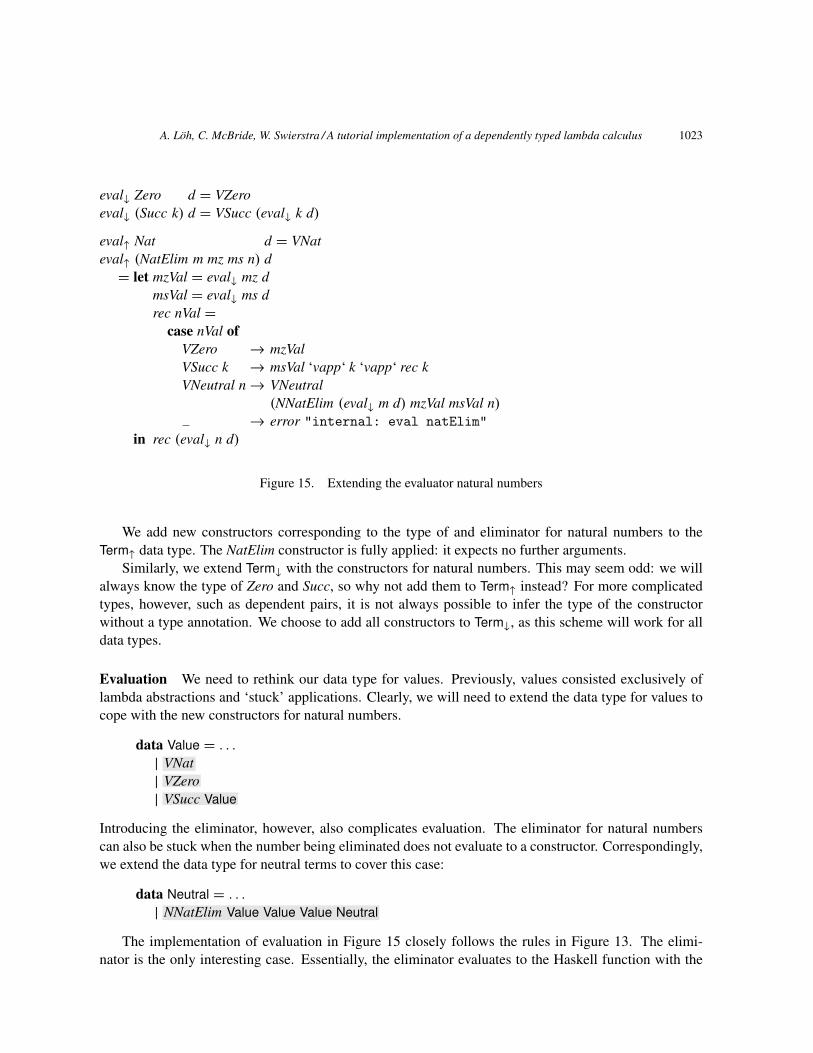
type↓ i 0 Zero VNat = return ()
type↓ i 0 (Succ k) VNat = type↓ i 0 k VNat
type↑ i 0 Nat = return VStartype↑ i 0 (NatElim m mz ms n) =
do type↓ i 0 m (VPi VNat (const VStar))let mVal = eval↓ m [ ]type↓ i 0 mz (mVal ‘vapp‘ VZero)
type↓ i 0 ms (VPi VNat (λk→ VPi (mVal ‘vapp‘ k) (λ → mVal ‘vapp‘ VSucc k)))type↓ i 0 n VNatlet nVal = eval↓ n [ ]return (mVal ‘vapp‘ nVal)
Figure 16. Extending the type checker for natural numbers
behaviour you would expect: if the number being eliminated evaluates to VZero, we evaluate the basecase mz; if the number evaluates to VSucc k, we apply the step function ms to the predecessor k and therecursive call to the eliminator; finally, if the number evaluates to a neutral term, the entire expressionevaluates to a neutral term. If the value being eliminated is not a natural number or a neutral term, thiswould have already resulted in a type error. Therefore, the final catch-all case should never be executed.
Typing Figure 16 contains the implementation of the type checker that deals with natural numbers.Checking that Zero and Succ construct natural numbers is straightforward.
Type checking the eliminator is bit more involved. Remember that the eliminator has the followingtype:
natElim :: ∀m :: Nat→ ∗. m Zero→ (∀k :: Nat.m k→ m (Succ k))→ ∀n :: Nat.m n
We begin by type checking and evaluating the motive m. Once we have the value of m, we type checkthe two branches. The branch for zero should have type m Zero; the branch for successors should havetype ∀k :: Nat.m k→ m (Succ k). Despite the apparent complication resulting from having to hand codecomplex types, type checking these branches is exactly what would happen when type checking a foldover natural numbers in Haskell. Finally, we check that the n we are eliminating is actually a naturalnumber. The return type of the entire expression is the motive, accordingly applied to the number beingeliminated.
Other functions To complete the implementation of natural numbers, we must also extend the aux-iliary functions for substitution and quotations with new cases. All new code is, however, completelystraightforward, because no new binding constructs are involved.
A. Loh, C. McBride, W. Swierstra / A tutorial implementation of a dependently typed lambda calculus 1025
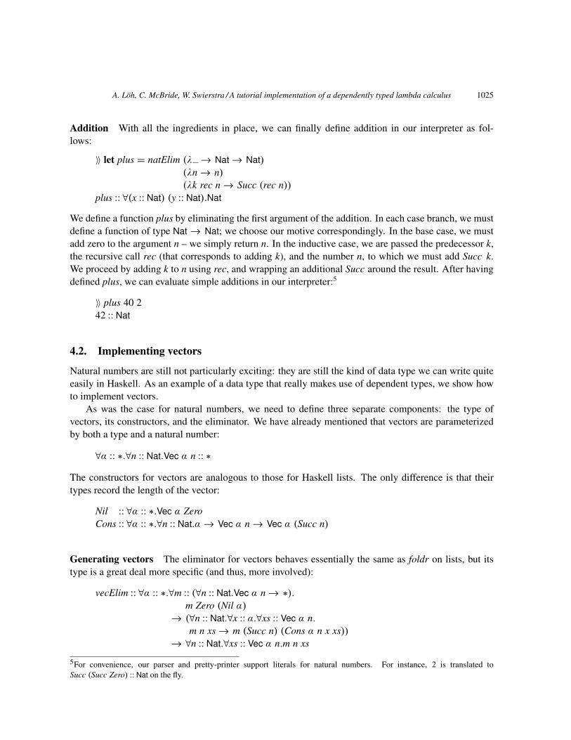
Addition With all the ingredients in place, we can finally define addition in our interpreter as fol-lows:
〉〉 let plus = natElim (λ → Nat→ Nat)(λn→ n)
(λk rec n→ Succ (rec n))
plus :: ∀(x :: Nat) (y :: Nat).Nat
We define a function plus by eliminating the first argument of the addition. In each case branch, we mustdefine a function of type Nat→ Nat; we choose our motive correspondingly. In the base case, we mustadd zero to the argument n – we simply return n. In the inductive case, we are passed the predecessor k,the recursive call rec (that corresponds to adding k), and the number n, to which we must add Succ k.We proceed by adding k to n using rec, and wrapping an additional Succ around the result. After havingdefined plus, we can evaluate simple additions in our interpreter:5
〉〉 plus 40 242 :: Nat
4.2. Implementing vectors
Natural numbers are still not particularly exciting: they are still the kind of data type we can write quiteeasily in Haskell. As an example of a data type that really makes use of dependent types, we show howto implement vectors.
As was the case for natural numbers, we need to define three separate components: the type ofvectors, its constructors, and the eliminator. We have already mentioned that vectors are parameterizedby both a type and a natural number:
∀α :: ∗.∀n :: Nat.Vec α n :: ∗
The constructors for vectors are analogous to those for Haskell lists. The only difference is that theirtypes record the length of the vector:
Nil :: ∀α :: ∗.Vec α ZeroCons :: ∀α :: ∗.∀n :: Nat.α→ Vec α n→ Vec α (Succ n)
Generating vectors The eliminator for vectors behaves essentially the same as foldr on lists, but itstype is a great deal more specific (and thus, more involved):
vecElim :: ∀α :: ∗.∀m :: (∀n :: Nat.Vec α n→ ∗).m Zero (Nil α)
→ (∀n :: Nat.∀x :: α.∀xs :: Vec α n.
m n xs→ m (Succ n) (Cons α n x xs))→ ∀n :: Nat.∀xs :: Vec α n.m n xs
5For convenience, our parser and pretty-printer support literals for natural numbers. For instance, 2 is translated toSucc (Succ Zero) :: Nat on the fly.
1026 A. Loh, C. McBride, W. Swierstra / A tutorial implementation of a dependently typed lambda calculus
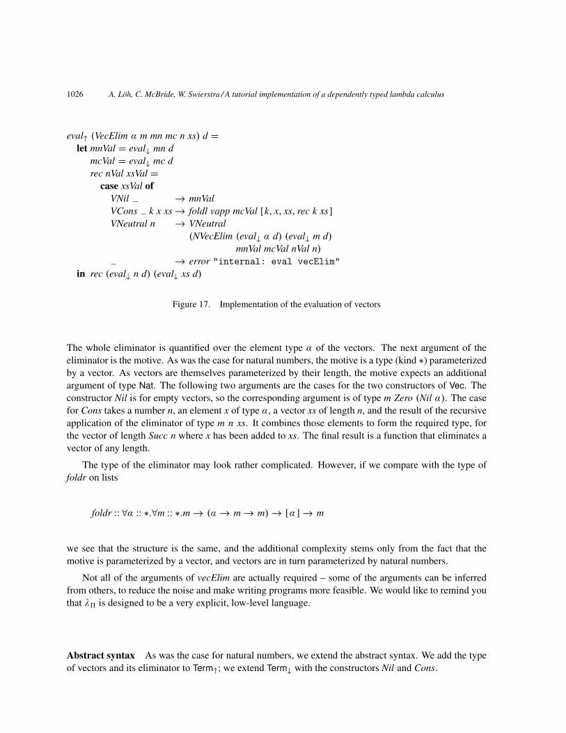
eval↑ (VecElim α m mn mc n xs) d =let mnVal = eval↓ mn d
mcVal = eval↓ mc drec nVal xsVal =
case xsVal ofVNil → mnValVCons k x xs→ foldl vapp mcVal [k, x, xs, rec k xs]VNeutral n → VNeutral
(NVecElim (eval↓ α d) (eval↓ m d)
mnVal mcVal nVal n)
→ error "internal: eval vecElim"in rec (eval↓ n d) (eval↓ xs d)
Figure 17. Implementation of the evaluation of vectors
The whole eliminator is quantified over the element type α of the vectors. The next argument of theeliminator is the motive. As was the case for natural numbers, the motive is a type (kind ∗) parameterizedby a vector. As vectors are themselves parameterized by their length, the motive expects an additionalargument of type Nat. The following two arguments are the cases for the two constructors of Vec. Theconstructor Nil is for empty vectors, so the corresponding argument is of type m Zero (Nil α). The casefor Cons takes a number n, an element x of type α, a vector xs of length n, and the result of the recursiveapplication of the eliminator of type m n xs. It combines those elements to form the required type, forthe vector of length Succ n where x has been added to xs. The final result is a function that eliminates avector of any length.
The type of the eliminator may look rather complicated. However, if we compare with the type offoldr on lists
foldr :: ∀α :: ∗.∀m :: ∗.m→ (α→ m→ m)→ [α ]→ m
we see that the structure is the same, and the additional complexity stems only from the fact that themotive is parameterized by a vector, and vectors are in turn parameterized by natural numbers.
Not all of the arguments of vecElim are actually required – some of the arguments can be inferredfrom others, to reduce the noise and make writing programs more feasible. We would like to remind youthat λ5 is designed to be a very explicit, low-level language.
Abstract syntax As was the case for natural numbers, we extend the abstract syntax. We add the typeof vectors and its eliminator to Term↑; we extend Term↓ with the constructors Nil and Cons.
A. Loh, C. McBride, W. Swierstra / A tutorial implementation of a dependently typed lambda calculus 1027
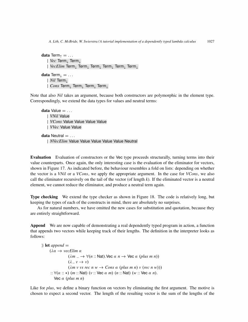
data Term↑ = . . .
| Vec Term↓ Term↓| VecElim Term↓ Term↓ Term↓ Term↓ Term↓ Term↓
data Term↓ = . . .
| Nil Term↓| Cons Term↓ Term↓ Term↓ Term↓
Note that also Nil takes an argument, because both constructors are polymorphic in the element type.Correspondingly, we extend the data types for values and neutral terms:
data Value = . . .
| VNil Value| VCons Value Value Value Value| VVec Value Value
data Neutral = . . .
| NVecElim Value Value Value Value Value Neutral
Evaluation Evaluation of constructors or the Vec type proceeds structurally, turning terms into theirvalue counterparts. Once again, the only interesting case is the evaluation of the eliminator for vectors,shown in Figure 17. As indicated before, the behaviour resembles a fold on lists: depending on whetherthe vector is a VNil or a VCons, we apply the appropriate argument. In the case for VCons, we alsocall the eliminator recursively on the tail of the vector (of length k). If the eliminated vector is a neutralelement, we cannot reduce the eliminator, and produce a neutral term again.
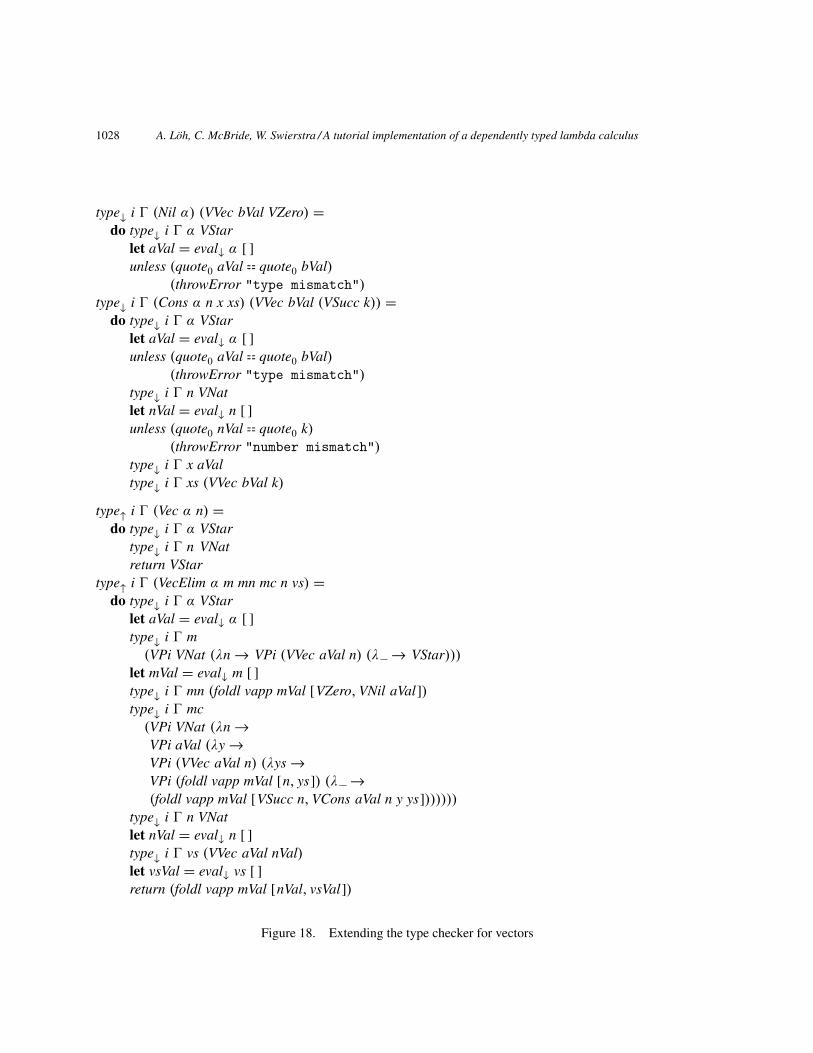
Type checking We extend the type checker as shown in Figure 18. The code is relatively long, butkeeping the types of each of the constructs in mind, there are absolutely no surprises.
As for natural numbers, we have omitted the new cases for substitution and quotation, because theyare entirely straightforward.
Append We are now capable of demonstrating a real dependently typed program in action, a functionthat appends two vectors while keeping track of their lengths. The definition in the interpreter looks asfollows:
〉〉 let append =(λα→ vecElim α
(λm → ∀(n :: Nat).Vec α n→ Vec α (plus m n))
(λ v→ v)(λm v vs rec n w→ Cons α (plus m n) v (rec n w)))
:: ∀(α :: ∗) (m :: Nat) (v :: Vec α m) (n :: Nat) (w :: Vec α n).
Vec α (plus m n)
Like for plus, we define a binary function on vectors by eliminating the first argument. The motive ischosen to expect a second vector. The length of the resulting vector is the sum of the lengths of the
1028 A. Loh, C. McBride, W. Swierstra / A tutorial implementation of a dependently typed lambda calculus
type↓ i 0 (Nil α) (VVec bVal VZero) =
do type↓ i 0 α VStarlet aVal = eval↓ α [ ]unless (quote0 aVal = = quote0 bVal)
(throwError "type mismatch")type↓ i 0 (Cons α n x xs) (VVec bVal (VSucc k)) =
do type↓ i 0 α VStarlet aVal = eval↓ α [ ]unless (quote0 aVal = = quote0 bVal)
(throwError "type mismatch")type↓ i 0 n VNatlet nVal = eval↓ n [ ]unless (quote0 nVal = = quote0 k)
(throwError "number mismatch")type↓ i 0 x aValtype↓ i 0 xs (VVec bVal k)
type↑ i 0 (Vec α n) =
do type↓ i 0 α VStartype↓ i 0 n VNatreturn VStar
type↑ i 0 (VecElim α m mn mc n vs) =do type↓ i 0 α VStar
let aVal = eval↓ α [ ]type↓ i 0 m
(VPi VNat (λn→ VPi (VVec aVal n) (λ → VStar)))let mVal = eval↓ m [ ]type↓ i 0 mn (foldl vapp mVal [VZero, VNil aVal])type↓ i 0 mc
(VPi VNat (λn→VPi aVal (λy→VPi (VVec aVal n) (λys→VPi (foldl vapp mVal [n, ys]) (λ →
(foldl vapp mVal [VSucc n, VCons aVal n y ys]))))))type↓ i 0 n VNatlet nVal = eval↓ n [ ]type↓ i 0 vs (VVec aVal nVal)let vsVal = eval↓ vs [ ]return (foldl vapp mVal [nVal, vsVal])
Figure 18. Extending the type checker for vectors
A. Loh, C. McBride, W. Swierstra / A tutorial implementation of a dependently typed lambda calculus 1029
argument vectors plus m n. Appending an empty vector to another vector v results in v. Appending avector of the form Cons m v vs to a vector v works by invoking recursion via rec (which appends vs tow) and prepending v. Of course, we can also apply the function thus defined:
〉〉 assume (α :: ∗) (x :: α) (y :: α)
〉〉 append α 2 (Cons α 1 x (Cons α 0 x (Nil α)))
1 (Cons α 0 y (Nil α))
Cons α 2 x (Cons α 1 x (Cons α 0 y (Nil α))) :: Vec α 3
We assume a type α with two elements x and y, and append a vector containing two x’s to a vectorcontaining one y.
4.3. Discussion
In this section we have shown how to add two data types to our core theory: natural numbers andvectors. Using exactly the same principles, many more data types can be added. For example, for anynatural number n, we can define the type Fin n that contains exactly n elements. In particular, Fin 0, Fin 1and Fin 2 are the empty type, the unit type, and the type of booleans respectively. Furthermore, Fin canbe used to define a total projection function from vectors, of type
project :: ∀(α :: ∗) (n :: Nat).Vec α n→ Fin n→ α
Another interesting dependent type is the equality type
Eq :: ∀(α :: ∗).α→ α→ ∗
with a single constructor
Refl :: ∀(α :: ∗) (x :: α)→ Eq α x x
Using Eq, we can state and prove theorems about our code directly in λ5. For instance, the type
∀(α :: ∗) (n :: Nat).Eq Nat (plus n Zero) n
states that Zero is the right-neutral element of addition. Any term of that type serves as a proof of thattheorem, via the Curry-Howard isomorphism.
These examples and a few more are included with the interpreter in the article sources, which can bedownloaded via the λ5 homepage [6]. More about suitable data types for dependently typed languagesand writing dependently typed programs can be found in another tutorial [11].
Throughout this section, we have chosen to extend the abstract syntax of our language for every datatype we add. Alternatively, we could use the Church encoding of data types, e.g., representing naturalnumbers by the type ∀(α ::∗).α→ (α→ α)→ α. Although this choice may seem to require less effort,it does introduce some problems. Although we can use the Church encoding to write simple folds, wecannot write dependently typed programs that rely on eliminators without extending our theory further.This makes it harder to write programs with an inherently dependent type, such as our append function.As our core theory should be able to form the basis of a dependently typed programming language, wechose to avoid using such an encoding.
1030 A. Loh, C. McBride, W. Swierstra / A tutorial implementation of a dependently typed lambda calculus
5. Toward dependently typed programming
The calculus we have described is far from a real programming language. Although we can write, typecheck, and evaluate simple expressions there is still a lot of work to be done before it becomes feasibleto write large, complex programs. In this section, we do not strive to enumerate all the problems thatlarge-scale programming with dependent types must face, let alone solve them. Instead, we try to sketchhow a programming language may be built on top of the core calculus we have seen so far and point youto related literature.
As our examples illustrate, programming with eliminators does not scale. Epigram [14] uses a cleverchoice of motive to make programming with eliminators a great deal more practical [8, 13]. By choosingthe right motive, we can exploit type information when defining complicated functions. Eliminators maynot appear to be terribly useful, but they form the foundations on which dependently typed programminglanguages may be built.
Writing programs with complex types in one go is not easy. Epigram and Agda [17] allow pro-grammers to put ‘holes’ in their code, leaving parts of their programs undefined [18]. Programmers canthen ask the system what type a specific hole has, effectively allowing the incremental development ofcomplex programs.
As it stands, the core system we have presented requires programmers to explicitly instantiate poly-morphic functions. This is terribly tedious! Take the append function we defined: of its five arguments,only two are interesting. Fortunately, uninteresting arguments can usually be inferred. Many program-ming languages and proof assistants based on dependent types have support for implicit arguments thatthe user can omit when calling a function. Note that these arguments need not be types: the appendfunction is ‘polymorphic’ in the length of the vectors.
Finally, we should reiterate that the type system we have presented is unsound. As the kind of ∗ isitself ∗, we can encode a variation of Russell’s paradox, known as Girard’s paradox [2]. This allows usto create an inhabitant of any type. To fix this, the standard solution is to introduce an infinite hierarchyof types: the type of ∗ is ∗1, the type of ∗1 is ∗2, and so forth.
6. Discussion
There is a large amount of relevant literature regarding both implementing type systems and type theory.Pierce’s book [19] is an excellent place to start. Martin-Lof’s notes on type theory [7] are still highlyrelevant and form an excellent introduction to the subject. More recent books by Nordstrom et al. [16]and Thompson [20] are freely available online.
There are several dependently typed programming languages and proof assistants readily available.Coq [1] is a mature, well-documented proof assistant. While it is not primarily designed for dependentlytyped programming, learning Coq can help get a feel for type theory. Haskell programmers may feelmore at home using recent versions of Agda [17], a dependently typed programming language. Notonly does the syntax resemble Haskell, but functions may be defined using pattern matching and generalrecursion. Finally, Epigram [14, 11] proposes a more radical break from functional programming aswe know it. While the initial implementation is far from perfect, many of Epigram’s ideas are not yetimplemented elsewhere.
A. Loh, C. McBride, W. Swierstra / A tutorial implementation of a dependently typed lambda calculus 1031
Other implementations of the type system we have presented here have been published elsewhere [3,4]. These implementations are given in pseudocode and accompanied by a proof of correctness. Thefocus of our article is somewhat different: we have chosen to describe a concrete implementation as avehicle for explanation.
In the introduction we mentioned some of the concerns functional programmers have regarding de-pendent types. The type checking algorithm we have presented here is decidable and will always termi-nate. The phase distinction between evaluation and type checking becomes more subtle, but is not lost.The fusion of types and terms introduces new challenges, but also has a lot to offer. Most importantly,though, getting started with dependent types is not as hard as you may think. We hope to have whetyour appetite, guiding you through your first steps, but encourage you to start exploring dependent typesyourself!
Acknowledgements We would like to thank Thorsten Altenkirch, Lennart Augustsson, Isaac Dupree,Clemens Fruhwirth, Jurriaan Hage, Stefan Holdermans, Shin-Cheng Mu, Phil Wadler, the students fromthe autumn 2007 seminar on Type Systems at Utrecht University, the Lambda the Ultimate-community,and the anonymous referees for their helpful comments on a previous version of this article.
References
[1] Bertot, Y., Casteran, P.: Interactive Theorem Proving and Program Development. Coq’Art: The Calculus ofInductive Constructions, Springer Verlag, 2004.
[2] Coquand, T.: An analysis of Girard’s paradox, First IEEE Symposium on Logic in Computer Science, 1986.
[3] Coquand, T.: An Algorithm for Type-Checking Dependent Types, Science of Computer Programming, 26(1-3), 1996, 167–177.
[4] Coquand, T., Takeyama, M.: An Implementation of Type: Type, International Workshop on Types for Proofsand Programs, 2000.
[5] Hinze, R., Loh, A.: lhs2TEX, 2007, http://www.cs.uu.nl/~andres/lhs2tex.
[6] λ5 homepage, 2007, http://www.cs.uu.nl/~andres/LambdaPi.
[7] Martin-Lof, P.: Intuitionistic type theory, Bibliopolis, 1984.
[8] McBride, C.: Dependently Typed Functional Programs and their Proofs, Ph.D. Thesis, University of Edin-burgh, 1999.
[9] McBride, C.: Elimination with a Motive, TYPES ’00: Selected papers from the International Workshop onTypes for Proofs and Programs, Springer-Verlag, 2000.
[10] McBride, C.: Faking it: Simulating Dependent Types in Haskell, Journal of Functional Programming, 12(5),2002, 375–392.
[11] McBride, C.: Epigram: Practical Programming with Dependent Types., Advanced Functional Programming,2004.
[12] McBride, C., McKinna, J.: Functional pearl: I am not a number – I am a free variable, Haskell ’04: Proceed-ings of the 2004 ACM SIGPLAN workshop on Haskell, 2004.
[13] McBride, C., McKinna, J.: The view from the left, Journal of Functional Programming, 14(1), 2004, 69–111.
1032 A. Loh, C. McBride, W. Swierstra / A tutorial implementation of a dependently typed lambda calculus
[14] McBride, C. et al.: Epigram, 2004, http://www.e-pig.org.
[15] Meijer, E., Fokkinga, M., Paterson, R.: Functional Programming with Bananas, Lenses, Envelopes andBarbed Wire, 5th Conf. on Functional Programming Languages and Computer Architecture, 1991.
[16] Nordstrom, B., Petersson, K., Smith, J. M.: Programming in Martin-Lof’s Type Theory: An Introduction,Clarendon, 1990.
[17] Norell, U.: Agda 2, http://appserv.cs.chalmers.se/users/ulfn/wiki/agda.php.
[18] Norell, U., Coquand, C.: Type checking in the presence of meta-variables, Submitted to Typed LambdaCalculi and Applications 2007.
[19] Pierce, B. C.: Types and Programming Languages, MIT Press, Cambridge, MA, USA, 2002, ISBN 0-262-16209-1.
[20] Thompson, S.: Type Theory and Functional Programming, Addison Wesley Longman Publishing Co., Inc.,1991.


![Bidirectional Elaboration of Dependently Typed Programsfferre8/papers/BidirectionalElaboration.pdfIdris, Brady [2013] describes the elaboration between source and target, but no theoretical](https://img.pdfslide.us/doc/110x75/5f77106973e3b54c1e1d3d03/bidirectional-elaboration-of-dependently-typed-programs-fferre8papersbidirectionalelaborationpdf.jpg)


![Intrinsically-Typed Definitional Interpreters for ... · Reynolds2004], at least for pure, functional object languages, is to use a dependently-typed host language, such as Agda [Norell2007],](https://img.pdfslide.us/doc/110x75/5f77085ae69ef54e0061e7db/intrinsically-typed-definitional-interpreters-for-reynolds2004-at-least-for.jpg)


![Idris 2: Quantitative Type Theory in Action · 2020-03-04 · concurrent programming with session types. 1 INTRODUCTION Dependently typed programming languages, such as Idris [Brady2013],](https://img.pdfslide.us/doc/110x75/5f7707ff0247e23a547cb7c0/idris-2-quantitative-type-theory-in-action-2020-03-04-concurrent-programming.jpg)