A Tutorial Guide to Mixed-Integer ProgrammingModels and Solution Techniques

J. Cole Smith and Z. Caner TaskınDepartment of Industrial and Systems Engineering

University of FloridaGainesville, FL 32611

cole@ise.ufl.edu, taskin@ufl.edu

March 26, 2007

Abstract

Mixed-integer programming theory provides a mechanism for optimizing decisionsthat take place in complex systems, including those encountered in biology and medicine.This chapter is intended for researchers and practitioners wanting an introduction tothe field of mixed-integer programming. We begin by discussing basic mixed-integerprogramming formulation principles and tricks, especially with regards to the use of bi-nary variables to form logical statements. We then discuss two core techniques, branch-and-bound and cutting-plane algorithms, used to solve mixed-integer programs. Weillustrate the use of mixed-integer programming in the context of several medical ap-plications, and close with a featured study on Intensity Modulated Radiation Therapyplanning.

1 Introduction

This chapter describes the use of mixed-integer programming in optimizing complex systems,such as those arising in biology, medicine, transportation, telecommunications, sports, andnational security. Consider, for instance, an emergency that results in 100 injuries. Atriage center is established to administer first aid and assign victims to one of three nearbyhospitals, each of which is capable of handling a limited number of patients. Each hospitalmay have varying equipment and staff levels, and each will be located at a different distancefrom the emergency. The optimization problem that arises is to assign patients to hospitalsin a way that maximizes the effectiveness of care that can be given to the victims, whileobeying physical capacity restrictions imposed by the hospitals. Experts often attempt tosolve these problems based on intuition and experience, but the resulting solution is almostinvariably suboptimal due to the inherent complexities of such problems. In applications ofcritical importance, there is sufficient motivation to turn to mathematical techniques thatcan provably obtain a “best” solution.

1

Mixed-integer programming is a subset of the broader field of mathematical programming.Mathematical programming formulations include a set of variables, which represent actionsthat can be taken in the system being modelled. One then attempts to optimize (eitherin the minimization or maximization sense) a function of these variables, which maps eachpossible set of decisions into a single score that assesses the quality of the solution. Thesescores are often in units of currency representing total cost incurred or revenue gained. Thelimitations of the system are included as a set of constraints, which are usually stated byrestricting functions of the decision variables to be equal to, not more than, or not less than,a certain numerical value. Another type of constraint can simply restrict the set of valuesto which a variable might be assigned.

Several applications involve decisions that are discrete (e.g., to which hospital an emer-gency patient should be assigned), while some other decisions are continuous in nature (e.g.,determining the dosage of fluids to be administered to a patient). On the surface, the abilityto enumerate all possible values that a discrete decision can take seems appealing; however,in most applications, the discrete variables are interrelated, requiring an enumeration of allcombinations of values that the entire set of discrete variables can take.

What are the implications of complete enumeration techniques on processing time? Sup-pose that there exist n variables, each of which can take on a value of zero or one. Fur-thermore, suppose that each configuration of these variables can be evaluated (tested forfeasibility to the problem constraints and scored) using n computer operations. Since thereare 2 choices for each variable, there are 2n configurations. Even if we are using a computercapable of processing 10 trillion operations per second (or 10 teraflops, and at the time ofthis writing, only 58 of the world’s top 500 supercomputers are capable of such a feat), ifn = 50, the computer will take 1.5 hours to finish enumerating all possibilities. One mightbe tempted to simply let the computer run all night if need be for important problems, andwhile this is indeed valid for the case in which n = 50, the computational growth rate forthese problems is astounding: for n = 60, the computer will require 80 days to terminate,and for n = 70, the computer will require 262 years. Another question regards the evolutionof computing speed, noting that faster computers are constantly emerging. If the programmust be finished within two hours, the current 10 teraflop machine will permit the solutionof problems with n = 50. If a quantum leap is discovered that results in the invention of10,000 teraflop machine, this fictional computer would only be able to handle problems withn = 60 within two hours. Computer speedups, however impressive, are simply no match forexponential enumeration problems.

Therefore, a more efficient technique is required to solve problems containing discretevariables. Mixed-integer programming techniques do not explicitly examine every possiblecombination of discrete solutions, but instead examine a subset of possible solutions, and useoptimization theory to prove that no other solution can be better than the best one found.This type of technique is referred to as implicit enumeration.

This chapter is not a thorough review of integer programming literature, but is intendedfor technical researchers who may or may not have any familiarity with linear programming,but who are looking for an entry-level introduction to modelling and solution via integerand mixed-integer programming. The text by Wolsey [18] provides an accessible accountof fundamental integer programming methods and theory, while the updated classical workof Nemhauser and Wolsey [11] discusses integer programming and combinatorial theory in

2

detail.We discuss the general form of mixed-integer programming problems in Section 2, and

provide general tips for formulating problems as mixed-integer programs. A brief discussionof the branch-and-bound implicit enumeration technique for solving mixed-integer programs,as is relevant to practitioners, is given in Section 3. Next, Section 4 provides an exampleof mixed-integer programs in a real radiation therapy application, illustrating the materialpresented in the prior two sections. Finally, we conclude this chapter in Section 5.

2 Modelling Principles

We begin this section by discussing the general form of linear and mixed-integer program-ming problems in Section 2.1. We then give common steps and principles behind modellingproblems of this form in Section 2.2, and suggest a few common ways that mixed-integervariables can be used to model complex conditions arising in real-world scenarios.

2.1 General Form

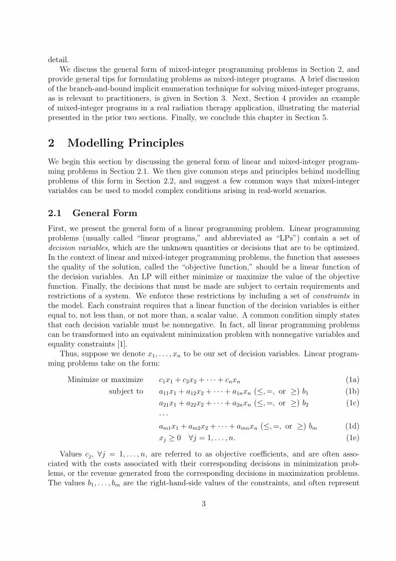
First, we present the general form of a linear programming problem. Linear programmingproblems (usually called “linear programs,” and abbreviated as “LPs”) contain a set ofdecision variables, which are the unknown quantities or decisions that are to be optimized.In the context of linear and mixed-integer programming problems, the function that assessesthe quality of the solution, called the “objective function,” should be a linear function ofthe decision variables. An LP will either minimize or maximize the value of the objectivefunction. Finally, the decisions that must be made are subject to certain requirements andrestrictions of a system. We enforce these restrictions by including a set of constraints inthe model. Each constraint requires that a linear function of the decision variables is eitherequal to, not less than, or not more than, a scalar value. A common condition simply statesthat each decision variable must be nonnegative. In fact, all linear programming problemscan be transformed into an equivalent minimization problem with nonnegative variables andequality constraints [1].

Thus, suppose we denote x1, . . . , xn to be our set of decision variables. Linear program-ming problems take on the form:

Minimize or maximize c1x1 + c2x2 + · · · + cnxn (1a)

subject to a11x1 + a12x2 + · · · + a1nxn (≤, =, or ≥) b1 (1b)

a21x1 + a22x2 + · · · + a2nxn (≤, =, or ≥) b2 (1c)

· · ·am1x1 + am2x2 + · · · + amnxn (≤, =, or ≥) bm (1d)

xj ≥ 0 ∀j = 1, . . . , n. (1e)

Values cj, ∀j = 1, . . . , n, are referred to as objective coefficients, and are often asso-ciated with the costs associated with their corresponding decisions in minimization prob-lems, or the revenue generated from the corresponding decisions in maximization problems.The values b1, . . . , bm are the right-hand-side values of the constraints, and often represent

3

amounts of available resources (especially for ≤ constraints) or requirements (especially for≥ constraints). The aij-values thus typically denote how much of resource/requirement i isconsumed/satisfied by decision j.

Note that nonlinear terms are not allowed in the model, prohibiting for instance themultiplication of two decision variables, the maximum of several variables, or the absolutevalue of a variable. (These conditions are often desired, but must be achieved by differenttechniques.) Also, any inequalities present in the model are never strict.

Problems of the form (1) are called “linear programs” because the objective function andconstraint functions are all linear. Integer programs (IPs) are stated in an identical fashion,except that all decision variables are constrained to take on integer values. (Hence, integerprograms are sometimes called “integer linear programs.”) A mixed-integer program (MIP)is a linear program with the added restriction that some, but not necessarily all, of thevariables must be integer-valued. Several studies also replace the term “integer” with “0-1”or “binary” when variables are restricted to take on either 0 or 1 values. For the purposesof this chapter, we focus on MIPs, with IPs being modelled and solved as a special case ofMIPs.

A solution that satisfies all constraints is called a feasible solution. Feasible solutionsthat achieve the best objective function value (according to whether one is minimizing ormaximizing) are called optimal solutions. Sometimes no solution exists to an MIP, and theMIP itself is called infeasible. On the other hand, some feasible MIPs have no optimalsolution, because it is possible to achieve infinitely good objective function values withfeasible solutions. Such problems are called unbounded.

2.2 Modelling Mixed-Integer Programming Problems

The modelling of complex systems using mixed-integer programs is often more of an artthan a science. Typically, a three-step looped process is used to model MIPs. The first stepinvolves defining a set of decision variables that represent choices that must be optimizedin the system. The second step usually involves the statement of constraints in the model,with the third step requiring the statement of an objective function (although the last twosteps can be done in either order).

It is very common, though, to recognize during model construction that the initial setof decision variables defined for the model are inadequate. Often, decision variables thatseem to be implied consequences of other actions must also be defined. The addition ofnew variables after an unsuccessful attempt at formulating constraints and objectives is the“loop” in the process.

The correct definition of decision variables can be especially complicated in modellingwith integer variables. If one is allowed to use binary variables in a formulation, it is possibleto represent yes-or-no decisions, enforce if-then statements, and even permit some sorts ofnonlinearity in the model (which can be transformed to an equivalent mixed-integer linearprogram).

To illustrate the modelling process, we consider the following three example systems.

Example 1. An outbreak of an infectious disease has been observed in a set N of locations.There exists a set M of teams capable of investigating these outbreaks. Team i ∈ M can

4

conclude its investigation of the outbreak in location j ∈ N in tij hours. Each team caneither investigate zero, one, or two outbreaks. If a team investigates two outbreaks, theymust travel from one location to the next. The travel time from location j1 ∈ N to locationj2 ∈ N is dj1j2 . Once all outbreaks have been investigated, a disease control center can takeaction to combat the outbreak. The goal is to minimize the amount of time necessary tocomplete the investigation of all locations. 2

Example 2. A medical practice is attempting to acquire a certain drug from a set Mof suppliers. The practice wishes to have a stock of dt units of this drug in month t, fort = 1, . . . , t. Purchasing one unit of the drug from supplier i ∈ M during time periodt ∈ {1, . . . , t} costs cit dollars. However, in order to purchase drugs from supplier i ∈ M ,at any time period, the practice must purchase a minimum of `i units of the drug duringthat time period. Fortunately, the practice has room for h units of inventory, and so at mosth units of the drug can be stored from one period to the next. If the practice finds itselfwith too many units of the drug, it can simply throw away the extra supply. The goal is tominimize the cost required to purchase the drugs for time periods 1, . . . , t. 2

Example 3. A nurse is assigned a set N of patients. For each patient i ∈ N , the nursemust spend pi minutes examining the patient. The nurse must then wait somewhere between`i and ui minutes before checking up on the patient, which requires qi minutes. The nurse,of course, cannot be in two places at the same time, although we will assume for simplicitythat the travel time to walk from one patient’s room to another is zero. The objective is tominimize the total amount of time required to tend to all patients. For instance, supposethat N contains three patients:

• Patient 1’s first visit lasts p1 = 5 minutes. The patient will then be checked on between`1 = 30 and u1 = 45 minutes later, after which the nurse will spend q1 = 5 more minutesof care on the second visit.

• Patient 2 needs p2 = 10 minutes of initial care, has an inter-care gap of `2 = 25 andu2 = 35 minutes, and requires q2 = 5 minutes of further care.

• Patient 3 needs p3 = 10 minutes of initial care, has an inter-care gap of `3 = 30 andu3 = 35 minutes, and requires q3 = 10 minutes of further care.

One solution would start treatment on patients 1, 2, and 3 in this order. The nurse’s schedulewould then be optimized according to the first column of Table 1 and the total treatmenttime would be 65 minutes. However, if the patients are treated in the opposite order, thetotal treatment time becomes only 60 minutes, as shown in the second column of Table 1.Indeed, the timing involved in this problem is quite difficult to optimize by hand. 2

Attempting to formulate any of these problems as an LP is problematic. With continuousvariables, the first example will likely end up assigning part of a team to one location,and part of a team to another location. The second one will not be able to represent theminimum purchase aspect of the problem. The third will not necessarily be able to keep thenurse from splitting attention simultaneously among multiple patients. Before attempting

5

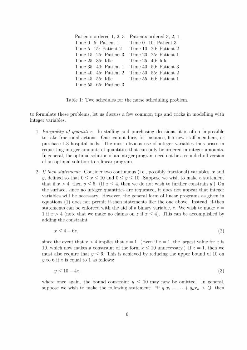
Patients ordered 1, 2, 3 Patients ordered 3, 2, 1Time 0−5: Patient 1 Time 0−10: Patient 3Time 5−15: Patient 2 Time 10−20: Patient 2Time 15−25: Patient 3 Time 20−25: Patient 1Time 25−35: Idle Time 25−40: IdleTime 35−40: Patient 1 Time 40−50: Patient 3Time 40−45: Patient 2 Time 50−55: Patient 2Time 45−55: Idle Time 55−60: Patient 1Time 55−65: Patient 3

Table 1: Two schedules for the nurse scheduling problem.

to formulate these problems, let us discuss a few common tips and tricks in modelling withinteger variables.

1. Integrality of quantities. In staffing and purchasing decisions, it is often impossibleto take fractional actions. One cannot hire, for instance, 6.5 new staff members, orpurchase 1.3 hospital beds. The most obvious use of integer variables thus arises inrequesting integer amounts of quantities that can only be ordered in integer amounts.In general, the optimal solution of an integer program need not be a rounded-off versionof an optimal solution to a linear program.

2. If-then statements. Consider two continuous (i.e., possibly fractional) variables, x andy, defined so that 0 ≤ x ≤ 10 and 0 ≤ y ≤ 10. Suppose we wish to make a statementthat if x > 4, then y ≤ 6. (If x ≤ 4, then we do not wish to further constrain y.) Onthe surface, since no integer quantities are requested, it does not appear that integervariables will be necessary. However, the general form of linear programs as given inequations (1) does not permit if-then statements like the one above. Instead, if-thenstatements can be enforced with the aid of a binary variable, z. We wish to make z =1 if x > 4 (note that we make no claims on z if x ≤ 4). This can be accomplished byadding the constraint

x ≤ 4 + 6z, (2)

since the event that x > 4 implies that z = 1. (Even if z = 1, the largest value for x is10, which now makes a constraint of the form x ≤ 10 unnecessary.) If z = 1, then wemust also require that y ≤ 6. This is achieved by reducing the upper bound of 10 ony to 6 if z is equal to 1 as follows:

y ≤ 10 − 4z, (3)

where once again, the bound constraint y ≤ 10 may now be omitted. In general,suppose we wish to make the following statement: “if q1x1 + · · · + qnxn > Q, then

6

r1x1 + · · · + rnxn ≤ R.” We would include the following conditions in our model:

q1x1 + · · · + qnxn ≤ Q + M ′z (4)

r1x1 + · · · + rnxn ≤ M ′′ − (M ′′ − R)z (5)

z binary, (6)

where M ′ and M ′′ are “sufficiently large” constants. These values should be just largeenough to not add unintentional restrictions to the model. For instance, we are notattempting to place any hard restriction on the quantity q1x1 + · · · + qnxn (writtenconveniently as q>x in vector form). If z = 1, the upper bound on q>x is Q + M ′,and hence M ′ must be large enough so that even if constraint (4) is removed from themodel, q>x would still never be more than Q+M ′. Likewise, if z = 0, we must choosea value M ′′ large enough in (5) such that r>x could never be more than M ′′ evenwithout the restriction (5). It is worth noting that assigning arbitrarily large valuesfor M ′ and M ′′ is not recommended, for reasons that will become more apparent inSection 3.

3. Enforce at least k out of p restrictions. This situation is similar to if-then constraints inthe way we model such restrictions. For a simple example, suppose we have nonnegativevariables x1, . . . , xn, and wish to require that at least three of these variables take onvalues of 5 or more. Then we can define variables z1, . . . , zn, such that if zj = 1,then xj ≥ 5, ∀j = 1, . . . , n. This simple if-then constraint can easily be modelled byemploying the following constraints:

xj ≥ 5zj ∀j = 1, . . . , n. (7)

Clearly, if zj = 1, then xj ≥ 5. If zj = 0, it is still possible for xj ≥ 5, but no suchrestrictions are enforced. We need to guarantee that three variables take on values of5 or more, and so we add the following “k-out-of-p” constraint:

z1 + . . . + zn = 3. (8)

Again, this constraint does not state that exactly three variables will be at least 5, butrather that at least three variables are guaranteed to be at least 5. This same trick canbe used to enforce the condition that at least k out of p sets of constraints are satisfied,and so on, often by using M -values as introduced in the section on if-then constraints.

4. Nonlinear product terms. In some circumstances, nonlinear terms can be transformedinto linear terms by the use of linear constraints. First, note that if xj is a binaryvariable, then xj = xq

j for any positive constant q. After that substitution is made,suppose that we have a nonlinear term of the form x1 ·x2 · · · xk ·y, where x1, . . . , xk arebinary variables and 0 ≤ y ≤ u is another variable, either continuous or integer. Thatis, all but perhaps one of the terms is a binary variable. First, replace the nonlinearterm with a single continuous variable, w. Using the if-then concept expressed above,note that if xj equals zero for any j ∈ {1, . . . , k}, then w equals zero as well. Also,

7

note that w can never be more than the upper bound, u, on the y-variable. Hence, weobtain the constraints

w ≤ uxj ∀j = 1, . . . , k. (9)

Of course, to guarantee that w equals zero in case any xj-variable equals to zero, wemust also state a nonnegativity constraint

w ≥ 0. (10)

Now, suppose that all x1 = · · · = xk = 1. In this case, we need to add constraints thatenforce the condition that w = y. Regardless of the x-variable values, w cannot bemore than y, and so we state the constraint

w ≤ y. (11)

However, in order to get the constraint “w ≥ y if x1 = · · · = xk = 1,” we include theconstraint

w ≥ u(x1 + · · · + xk − k) + y. (12)

If each x-variable equals to 1, then (12) states that w ≥ y, which along with (11)guarantees that w = y. On the other hand, if at least one xj = 0, j ∈ {1, . . . , k}, thenthe term u(x1 + · · · + xk − k) is not more than −u, and the right-hand-side of (12)is not positive; hence, (12) allows w to take on the correct value of zero (as would beenforced by (9) and (10)). As a final note, observe that even if y is an integer variable,we need not insist that w is an integer variable as well, since (9)−(12) guarantees thatw = x1 · · · xk · y, which must be an integer given integer x- and y-values.

Let us now briefly continue the examples introduced earlier in this section in the light ofthe modelling tricks introduced above.

Example 1, continued. Define binary decision variables xij, which equal one if teami ∈ M investigates an outbreak at location j ∈ N , and zero otherwise. Proceeding with thisinitial set of variables, we would then attempt to formulate the constraints of the problem.In fact, the only restrictions encountered thus far is the fact that each location must beinvestigated by exactly one team, the fact that each team can investigate no more than twolocations, and the fact that each x-variable must be binary. These constraints are respectivelygiven by: ∑

i∈M

xij = 1 ∀j ∈ N (13)∑j∈N

xij ≤ 2 ∀i ∈ M (14)

xij binary ∀i ∈ M, j ∈ N. (15)

Finally, we would attempt to formulate the objective function. Note that the amount of timerequired for team i ∈ M to complete their investigation(s) is the amount of time required

8

to perform the investigations,∑

j∈N tijxij, plus the travel time between location sites. Thistravel time can be represented by

∑all j1 6=j2∈N dj1j2xij1xij2 , noting that inter-location travel

time is required only if a team is required to visit both sites. The objective function has thefollowing form:

Minimize maximumi∈M

{∑j∈N

tijxij +∑

all j1 6=j2∈N

dj1j2xij1xij2

}.

This function is nonlinear for two reasons. One, the investigation completion time is a non-linear function due to the multiplication of x-variables. Two, the quantity being minimizedis the maximum of the teams’ investigation completion times.

At this point, we must add additional variables to the problem. Replace each nonlinearterm xij1xij2 with a new variable wij1j2 , and add linearization constraints

wij1j2 ≤ x1 similar to (9) (16a)

wij1j2 ≥ 0 similar to (10) (16b)

wij1j2 ≤ x2 similar to (11), treating x2 as “y” (16c)

wij1j2 ≥ x1 + x2 − 1 similar to (12). (16d)

The objective function now becomes:

Minimize maximumi∈M

{∑j∈N

tijxij +∑

all j1 6=j2∈N

dj1j2wij1j2

}.

In order to remove the “minimax” structure of this objective function, we rely on a com-mon trick for linear programming. First, we add a variable θ that represents the maximumcompletion time. We would then minimize θ, subject to the conditions that θ must be atleast as large as the completion time for team 1, θ must be at least as large as the completiontime for team 2, and so on, for each team. These constraints are:

θ ≥∑j∈N

tijxij +∑

all j1 6=j2∈N

dj1j2wij1j2 ∀i ∈ M. (17)

Of course, the question arises as to why θ will be equal to the maximum of the teams’completion times, since (17) merely enforces the condition that θ is at least as large as themaximum of these times. The answer is that the objective function will minimize θ, andso θ will take on the smallest possible value permitted by (17), which will indeed be themaximum of completion times.

The overall model is then given by:

Minimize θ

subject to Constraints (13) − (17).

9

Example 2, continued. An initial attempt at modelling this problem would define deci-sion variables xit, ∀i ∈ M, t = 1, . . . , t, equal to the amount of drugs purchased from supplieri in period t. It is also necessary in general to define variables gi, ∀i ∈ M , which denote howmany units of drugs are thrown away after period i (because we purchased too many from asupplier due to minimum purchase limits, and perhaps also due to inventory limits). How-ever, we must ensure that the number of drugs purchased from supplier i ∈ M at any timeperiod is either zero or at least `i. Hence, let us define binary decision variables zit, whichequal one if we purchase any supplies from supplier i ∈ M at time period t ∈ {1, . . . , t}, andzero otherwise.

However, stating the demand and inventory constraints is awkward (though possible)without another set of variables. Note that we must require

∑i∈M xi1 − g1 ≥ d1 in order to

satisfy period 1 demand. In period 2, we have that the inventory plus the amount of drugsordered in period 2, minus whatever is thrown away after period 2, must be at least d2.This condition is stated as ((

∑i∈M xi1 − g1) − d1) +

∑i∈M xi2 − g2 ≥ d2. For period 3, this

constraint becomes (((∑

i∈M xi1 − g1) − d1) + (∑

i∈M xi2 − g2) − d2) +∑

i∈M xi3 − g3 ≥ d3.It is evident that the expression quickly becomes quite large as the time period t increases.

Instead, we can define inventory variables yt, for t = 1, . . . , t, which represent the amountof drug inventory remaining after period t. From this point, it is easier to establish “flowbalance” constraints, which state that the amount of drugs coming into the practice at eachperiod (inventory from the previous period, plus amount purchased from suppliers duringthe current period) equals to the drugs that leave the practice at the current period (thosedemanded by patients, plus those put into inventory after the period, plus those thrownaway). These balance constraints are given as

yt−1 +∑i∈M

xit = dt + yt + gt ∀t = 1, . . . , t, (18)

where y0 is defined to be zero. The minimum purchase quantity constraints are given as

xit ≥ `izit ∀i ∈ M, t = 1, . . . , t (19)

xit ≤ Mitzit ∀i ∈ M, t = 1, . . . , t, (20)

where Mit is a sufficiently large constant, ∀i, t. If zit = 1, then `i ≤ xit ≤ Mit, whileif zit = 0, then xit = 0. A possible value for Mit would be the maximum of `i and the

remaining demands∑t

u=t du. Finally, we require constraints that state bounds on the x-, g-,and z-variables.

xit ≥ 0, and zit binary ∀i ∈ M, t = 1, . . . , t (21)

0 ≤ yt ≤ h and gt ≥ 0 ∀t = 1, . . . , t. (22)

The overall formulation can now be stated as:

Minimize∑i∈M

t∑t=1

citxit (23)

subject to Constraints (18) − (22).

10

Example 3, continued. There exist several methods of modelling and solving this prob-lem. One technique defines a continuous variable fi to be the first time that the nurse seespatient i ∈ N , and si to be the second time that the nurse sees patient i ∈ N . These variabledefinitions allow us to state the minimum and maximum gaps between the first and secondvisits by the nurse:

si − (fi + pi) ≥ `i ∀i ∈ N (24)

si − (fi + pi) ≤ ui ∀i ∈ N. (25)

However, we must now enforce the restriction that the nurse does not tend to two or morepatients at the same time. We must ensure that for each pair of nurse visits (first visits todifferent patients, first and second visits to different patients, and second visits to differentpatients), one visit starts before the other begins, or vice versa. (The two visits to the samepatient are disjoint due to (24).)

Define binary variables z11ij to equal one if the first visit to patient i ∈ N occurs before

the first visit to patient j ∈ N , and zero otherwise. Also, define z12ij if the first visit to patient

i ∈ N occurs before the second visit to patient j ∈ N , and zero otherwise. Similarly, z21ij

relates the second visit of patient i ∈ N to the first visit of patient j ∈ N , and z22ij relates the

second visit of patient i ∈ N to the second visit of patient j ∈ N . The following constraintsrelate the z-variables to the f - and s-variables.

fj − (fi + pi) ≥ −M11ij (1 − z11

ij ) ∀i, j ∈ N, i 6= j (26)

sj − (fi + pi) ≥ −M12ij (1 − z12

ij ) ∀i, j ∈ N, i 6= j (27)

fj − (si + qi) ≥ −M21ij (1 − z21

ij ) ∀i, j ∈ N, i 6= j (28)

sj − (si + qi) ≥ −M22ij (1 − z22

ij ) ∀i, j ∈ N, i 6= j, (29)

where the M -values once again are sufficiently large constants. For instance, (26) states thatif z11

ij = 1, then fj ≥ fi + pi, meaning that the nurse finishes the visit to patient i before thevisit to patient j occurs. We now need to state constraints ensuring that one visit finishesbefore the next one starts, or vice versa.

z11ij + z11

ji = 1 ∀i, j ∈ N, i < j (30)

z22ij + z22

ji = 1 ∀i, j ∈ N, i < j (31)

z12ij + z21

ji = 1 ∀i, j ∈ N, i 6= j. (32)

Constraints (30) and (31) respectively ensure that no pair of first visits and no pair ofsecond visits overlap. Constraints (32) ensure that no pair of first/second visits overlaps.(In fact, the number of z-variables in the model can now be halved by substituting out z-variables according to (30), (31), and (32). However, we retain these variables here for easeof exposition.)

Finally, we again have a minimax objective in which the time of the final patient visitmust be minimized. Again, we define θ to be the time of the final patient visit, which must

11

equal to si + qi, for some i ∈ N . The final model is then given as:

Minimize θ (33)

subject to Constraints (24) − (32)

θ ≥ si + qi ∀i ∈ N (34)

si, fi ≥ 0 ∀i ∈ N (35)

z11ij , z12

ij , z21ij , z22

ij binary ∀i, j ∈ N, i 6= j. (36)

This problem is in fact adapted from a study on radar pulse interleaving, which containssimilar challenges to this nurse scheduling problem. See [4, 6, 16] for a more thoroughexamination of interleaving applications and integer programming techniques.

3 MIP Solution Techniques

Often, there are alternative ways of modelling optimization problems as MIPs. There some-times exist trade-offs in these different modelling approaches. Some models may be smaller(in terms of the number of constraints and variables required), but may be more difficult tosolve than larger models. In fact, the difference can be significant, and can make a differencein whether or not MIPs can be solved quickly enough to be practically useful. (For instance,the situation described in Example 1 mentioned in the previous section must be solved beforethe outbreak spreads!)

Improving the efficiency of solving MIP models requires an understanding of how MIPsolvers work. Premium MIP solvers, such as CPLEX (ILOG, Inc.), Xpress-MP (Dash Op-timization), SYMPHONY and CBC (COIN-OR project), and Solver (Frontline Systems,Inc.), employ a combination of branch-and-bound and cutting-plane techniques. While areview of how to use these software packages is well beyond the scope of this tutorial, it isimportant to understand the basics of MIP solution algorithms in order to understand thekey principles in MIP modelling.

For the rest of this section, assume that we are solving a minimization MIP. (Maximiza-tion MIPs are solved in much the same fashion.) To help illustrate the branch-and-boundprocess, we consider the following example MIP (actually a pure IP since all variables areinteger).

Minimize 4x1 + 6x2 (37a)

subject to 2x1 + 2x2 ≥ 5 (37b)

x1 − x2 ≤ 1 (37c)

x1, x2 ≥ 0 and integer. (37d)

The first concept that we discuss in solving MIPs is that of relaxations. A relaxation ofan MIP is a problem such that (a) any solution to the MIP corresponds to a feasible solutionto the relaxed problem, and (b) each solution to the MIP has an objective function valuegreater than or equal to that of the corresponding solution to the relaxed problem. Themost commonly used relaxation for an MIP is its LP relaxation, which is identical to theMIP with the exception that variable integrality restrictions are eliminated. Clearly, any

12

integer-feasible solution to the MIP is also a solution to its LP relaxation, with matchingobjective function values.

Envision a bag containing several orange and blue marbles. Each marble represents asolution to the LP relaxation, but only the orange marbles also represent solutions to theMIP. Each marble has a weight, corresponding to its objective function value. The task inlinear programming is to find the lightest marble. The task in solving an MIP is to find thelightest orange marble.

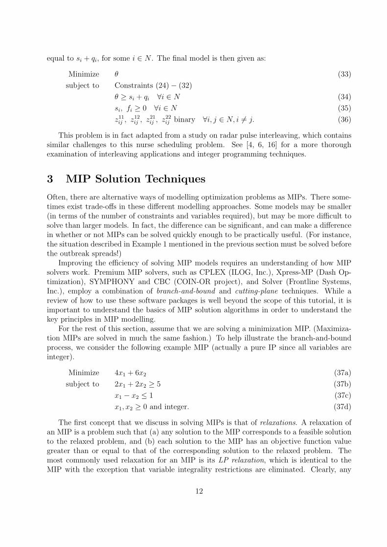
When describing the branch-and-bound algorithm for MIPs, it is helpful to know howLPs are solved. See [1, 8, 15, 17] for an explanation of linear programming theory andmethodology. For the purposes of this chapter, we simply note that linear programs can besolved quickly (in time bounded by a polynomial of the problem’s input size). Graphically,Figure 1 illustrates the feasible region (set of all feasible solutions) to the LP relaxation offormulation (37). Note that the gradient of the objective function is (4,6) (taken from thecoefficients of (37a)). This means that the objective function is increasing in this direction,and hence we wish to follow the direction (−4,−6) as far as possible in the feasible region.Put another way, think of (−4,−6) as the direction of gravity, and place a pebble in thefeasible region. The point to which the pebble falls, (1.75, 0.75), is the optimal solution tothe LP relaxation, and has an objective function value of 11.5.

Returning to the bag of marbles analogy, solving the LP relaxation has yielded a bluemarble (fractional, not integer, solution) with a weight of 11.5. This implies that all orangemarbles have a weight of 11.5 or more, since weight of the lightest marble in the bag was11.5. (In general, we cannot claim that the optimal solution to the LP is unique, and sowe allow for the possibility that MIP solutions exist with an identical objective function tothe optimal LP solution.) The important result is that a lower bound on the optimal MIPsolution is obtained from the LP relaxation. No solution to the MIP (37) can be found withan objective function value less than 11.5.

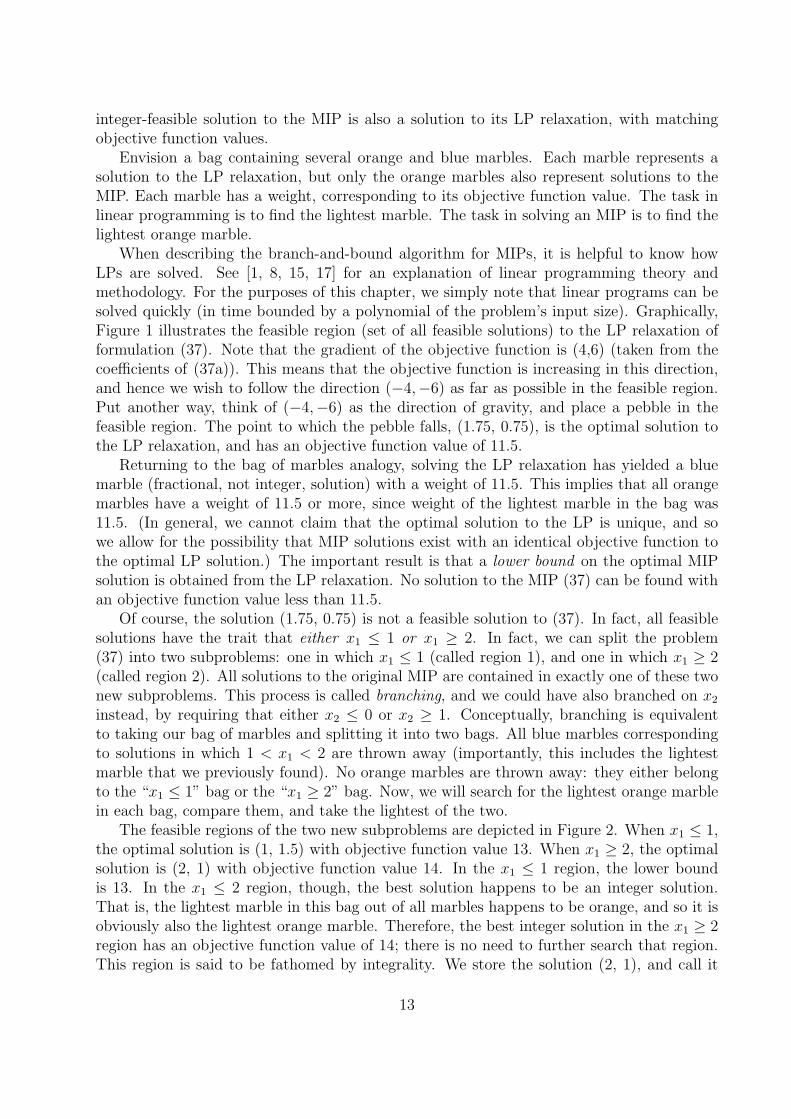
Of course, the solution (1.75, 0.75) is not a feasible solution to (37). In fact, all feasiblesolutions have the trait that either x1 ≤ 1 or x1 ≥ 2. In fact, we can split the problem(37) into two subproblems: one in which x1 ≤ 1 (called region 1), and one in which x1 ≥ 2(called region 2). All solutions to the original MIP are contained in exactly one of these twonew subproblems. This process is called branching, and we could have also branched on x2

instead, by requiring that either x2 ≤ 0 or x2 ≥ 1. Conceptually, branching is equivalentto taking our bag of marbles and splitting it into two bags. All blue marbles correspondingto solutions in which 1 < x1 < 2 are thrown away (importantly, this includes the lightestmarble that we previously found). No orange marbles are thrown away: they either belongto the “x1 ≤ 1” bag or the “x1 ≥ 2” bag. Now, we will search for the lightest orange marblein each bag, compare them, and take the lightest of the two.

The feasible regions of the two new subproblems are depicted in Figure 2. When x1 ≤ 1,the optimal solution is (1, 1.5) with objective function value 13. When x1 ≥ 2, the optimalsolution is (2, 1) with objective function value 14. In the x1 ≤ 1 region, the lower boundis 13. In the x1 ≤ 2 region, though, the best solution happens to be an integer solution.That is, the lightest marble in this bag out of all marbles happens to be orange, and so it isobviously also the lightest orange marble. Therefore, the best integer solution in the x1 ≥ 2region has an objective function value of 14; there is no need to further search that region.This region is said to be fathomed by integrality. We store the solution (2, 1), and call it

13

Figure 1: Feasible region of the LP relaxation

14

Figure 2: Feasible regions of the subproblems

our incumbent solution. If no better solution is found, it will become our optimal solution.At this point, there is one active region (or “active node” in the context of branch-and-

bound trees, which we will describe shortly), which is region 1. An active region is one thathas not been branched on, and that must still be explored, because there is a possibility thatit contains a solution better than the incumbent solution. The initial region is not active,because we have branched on it. Region 2 is not active because we have found the bestinteger solution in that region. Region 1, however, is still active and must be explored. Thelower bound over this region is 13; thus, we know that the optimal solution to the entireproblem must have an objective function value somewhere between 13 and 14 (inclusive).We recursively divide region 1, in which x1 ≤ 1. Since the optimal solution in this regionwas (1, 1.5), we branch by creating two new subproblems: one in which both x1 ≤ 1 andx2 ≤ 1 (called region 3), and one in which both x1 ≤ 1 and x2 ≥ 2 (called region 4). Once

15

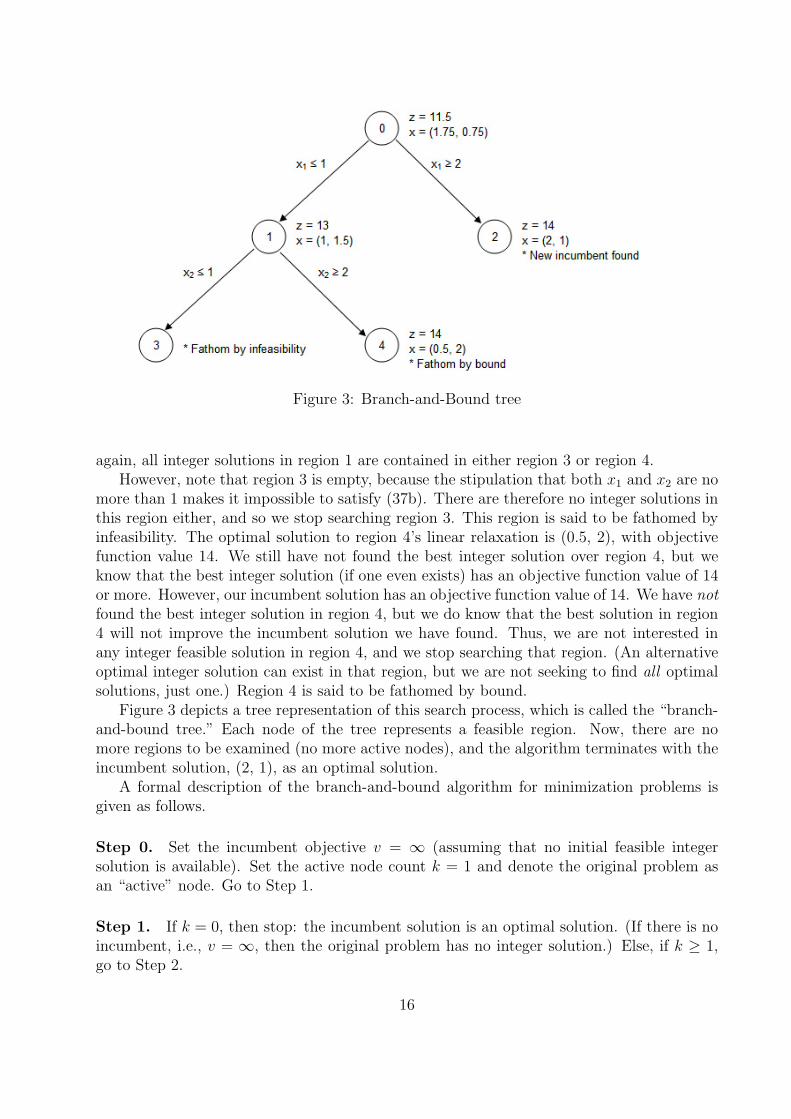
Figure 3: Branch-and-Bound tree

again, all integer solutions in region 1 are contained in either region 3 or region 4.However, note that region 3 is empty, because the stipulation that both x1 and x2 are no

more than 1 makes it impossible to satisfy (37b). There are therefore no integer solutions inthis region either, and so we stop searching region 3. This region is said to be fathomed byinfeasibility. The optimal solution to region 4’s linear relaxation is (0.5, 2), with objectivefunction value 14. We still have not found the best integer solution over region 4, but weknow that the best integer solution (if one even exists) has an objective function value of 14or more. However, our incumbent solution has an objective function value of 14. We have notfound the best integer solution in region 4, but we do know that the best solution in region4 will not improve the incumbent solution we have found. Thus, we are not interested inany integer feasible solution in region 4, and we stop searching that region. (An alternativeoptimal integer solution can exist in that region, but we are not seeking to find all optimalsolutions, just one.) Region 4 is said to be fathomed by bound.

Figure 3 depicts a tree representation of this search process, which is called the “branch-and-bound tree.” Each node of the tree represents a feasible region. Now, there are nomore regions to be examined (no more active nodes), and the algorithm terminates with theincumbent solution, (2, 1), as an optimal solution.

A formal description of the branch-and-bound algorithm for minimization problems isgiven as follows.

Step 0. Set the incumbent objective v = ∞ (assuming that no initial feasible integersolution is available). Set the active node count k = 1 and denote the original problem asan “active” node. Go to Step 1.

Step 1. If k = 0, then stop: the incumbent solution is an optimal solution. (If there is noincumbent, i.e., v = ∞, then the original problem has no integer solution.) Else, if k ≥ 1,go to Step 2.

16

Step 2. Choose any active node, and call it the “current” node. Solve the LP relaxationof the current node, and make it inactive. If there is no feasible solution, then go to Step 3.If the solution to the current node has objective value z∗ ≥ v, then go to Step 4. Else, if thesolution is all integer (and z∗ < v), then go to Step 5. Otherwise, go to Step 6.

Step 3. Fathom by infeasibility. Decrease k by 1 and return to Step 1.

Step 4. Fathom by bound. Decrease k by 1 and return to Step 1.

Step 5. Fathom by integrality. Replace the incumbent solution with the solution to thecurrent node. Set v = z∗, decrease k by 1, and return to Step 1.

Step 6. Branch on the current node. Select any variable that is fractional in the LPsolution to the current node. Denote this variable as xs and denote its value in the optimalsolution as f . Create two new active nodes: one by adding the constraint xs ≤ bfc to thecurrent node, and the other by adding xs ≥ dfe to the current node. Add 1 to k (two newactive nodes, minus one due to branching on the current node) and return to Step 1.

Note that in Step 0, we could run a heuristic procedure to quickly obtain a good-qualitysolution to the MIP with no guarantees on its optimality. This solution would then becomeour initial incumbent solution, and could possibly help conserve branch-and-bound memoryrequirements by increasing the rate at which active nodes are fathomed in Step 4. In Step 2,we may have several choices of active nodes on which to branch, and in Step 6, we may haveseveral choices on which variable to perform the branching operation. There has been muchempirical research designed to establish good general rules to make these choices, and theserules are implemented in commercial solvers. However, for specific types of formulations,one can often improve the efficiency of the branch-and-bound algorithm by experimentingwith node selection and variable branching rules.

The best-case scenario in solving a problem by branch-and-bound is that the originalnode yields an optimal LP solution that happens to be integer, and the algorithm termi-nates immediately. Indeed, in (37), if we simply add the constraint x1 +x2 ≥ 3 and solve theLP relaxation, we would obtain the optimal solution (2, 1) immediately. This also under-scores the importance of making the M -values introduced in the previous section as smallas possible. The smaller these M -values are, the fewer fractional solutions exist in the linearprogramming relaxation. Paying close attention to these M -values often results in significantimprovements in the computational efficiency of MIP algorithms.

Thus, a classical way to reduce the presence of fractional solutions is to find valid in-equalities, which do not cut off any integer solutions, but do cut off some fractional solutions.In terms of marbles, these inequalities remove some blue marbles from the bag, but neverorange marbles, and do so without branching into multiple bags. A cutting plane is a validinequality that removes the optimal LP relaxation solution from the feasible region. In the-ory, MIPs can be solved without branching either by (a) including enough valid inequalitiesbefore solving the LP relaxation, so that the LP relaxation provides an integer solution, or (b)

17

looping between solving the LP relaxation, adding a cutting plane, and re-solving the LP re-laxation, until the LP relaxation yields an integer solution. By themselves, these approachesare typically intractable and may suffer from numerical instability problems. However, themost effective implementations often use a combination of valid inequalities added a priorito the model, after which branch-and-bound is executed, with cutting planes periodicallyadded to the nodes of the branch-and-bound tree. This approach is called “branch-and-cut.”

Valid inequality and cutting-plane approaches can either be automatic or problem-specific.Classical automatic approaches are described by Nemhauser and Wolsey [11]. More relevantto the material in this chapter are problem-specific valid inequality generation techniques.For instance, in Example 2 in the previous section, suppose that the demand of drugs inperiods 1 and 2 is 100 units. Suppose that the minimum order quantity from each supplieris 150 units. If drugs become less expensive as time goes on, then the LP relaxation may tryto place only 2/3 of a minimum order in each period, so that only 100 drugs (instead of thefull complement of 150) are purchased in each period. Anticipating this class of fractionalsolutions, we note that at least one order must be placed in period 1 (since no orders resultin unsatisfied demand). This valid inequality is stated as∑

i∈M

zi1 ≥ 1. (38)

The addition of such inequalities to the MIP formulation often aid its performance, althoughoccasionally they make little difference, or even worsen the performance of the branch-and-bound solver. Negative impacts usually occur when the inclusion of extra valid inequalitiesmakes the formulation larger without sufficiently reducing its feasible region. Determiningwhich valid inequalities are computationally beneficial is usually a matter of trial-and-error.

4 Example Radiation Therapy Application

In this section we describe an application of mixed-integer programming in Intensity Mod-ulated Radiation Therapy (IMRT) planning. The underlying mechanism of radiotherapyis to radiate tumor tissues with high energy beams, which kill cancer cells. However, highenergy radiation also kills healthy tissues it passes through, possibly resulting in seriousdegradation in the patient’s quality of life. IMRT is a technique designed to help solve thisdilemma. IMRT delivers small amounts of doses from multiple beam angles, which intersectat tumor tissues. As a result, the tumor tissue receives enough radiation to kill the cancercells, but the healthy tissues are spared. The IMRT planning problem is usually solved inthree interdependent phases.

• Beam Angle Optimization (BAO): Selection of the beam angles to use

• Fluence Map Optimization (FMO): Determination of intensity profile to deliver fromeach beam angle

• Leaf Sequencing: Realization of the intensity profiles under the capabilities of availablemachinery

18

Planning problems in IMRT have been investigated by several researchers [2, 3, 12].The BAO problem can be formulated as an MIP model [9, 10]. The FMO problem canbe formulated as a large scale LP model [14] or a nonlinear programming model [13]. TheLeaf Sequencing problem can be formulated as an MIP model as we describe in this section.However, since the problem size of real-world IMRT instances is very large and these problemsare inherently complex, heuristic procedures are typically used to solve real instances in areasonable amount of time [5]. The reader is referred to [7] for a recent book chapter aboutmixed integer programming applications in IMRT. In this section, we will focus on the LeafSequencing problem and derive an MIP formulation for solving it optimally.

Leaf Sequencing Problem We are given an m × n matrix B that consists of integerscalled “beamlets.” Matrix B represents an intensity profile that needs to be delivered froma given beam angle. We need to find an optimal way of decomposing this matrix into a setof uniform-intensity shapes, in this case rectangles, that the available machinery can deliver.

Figure 4: Fluence map example

Figure 4 represents a small example fluence map. One way to decompose this map intodeliverable shapes is given in Figure 5. Define beam-on time as the amount of time requiredto deliver the doses prescribed by a set of deliverable shapes. In this problem, we measurethe beam-on time as the sum of doses. The solution represented in Figure 5 results in fourshapes and a total beam-on time of 9+4+6+1 = 20 time units. Assuming that the machinerequires 15 time units to switch from one shape to another, where time units are relative toone unit of beam-on time, the total time required by the configuration represented in Figure5 is 15 × 4 + 20 = 80 time units.

An alternative decomposition is given in Figure 6, resulting in only three shapes anda total beam-on time of only 9 time units. The total time for this decomposition is only15 × 3 + 9 = 54. This simple example illustrates that the total time required to deliveran intensity profile for a given beam varies significantly depending on the leaf sequence

Figure 5: Leaf sequence 1

19

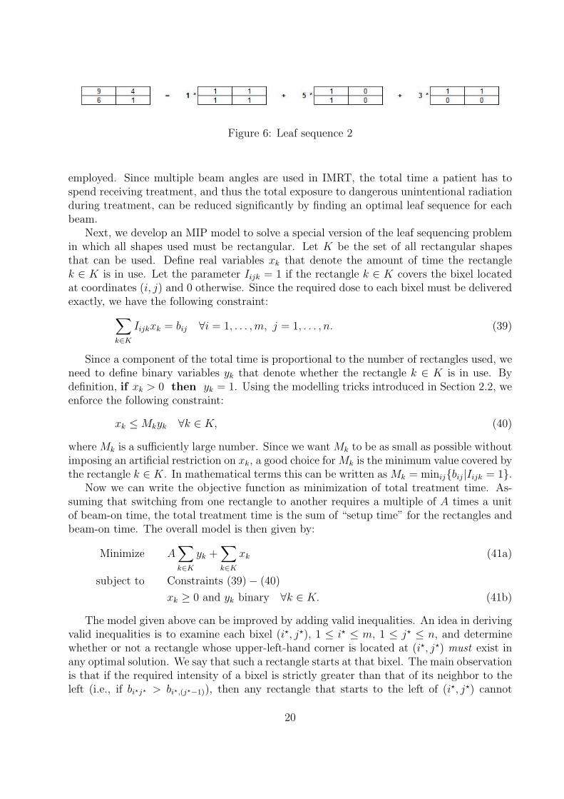
Figure 6: Leaf sequence 2

employed. Since multiple beam angles are used in IMRT, the total time a patient has tospend receiving treatment, and thus the total exposure to dangerous unintentional radiationduring treatment, can be reduced significantly by finding an optimal leaf sequence for eachbeam.

Next, we develop an MIP model to solve a special version of the leaf sequencing problemin which all shapes used must be rectangular. Let K be the set of all rectangular shapesthat can be used. Define real variables xk that denote the amount of time the rectanglek ∈ K is in use. Let the parameter Iijk = 1 if the rectangle k ∈ K covers the bixel locatedat coordinates (i, j) and 0 otherwise. Since the required dose to each bixel must be deliveredexactly, we have the following constraint:∑

k∈K

Iijkxk = bij ∀i = 1, . . . ,m, j = 1, . . . , n. (39)

Since a component of the total time is proportional to the number of rectangles used, weneed to define binary variables yk that denote whether the rectangle k ∈ K is in use. Bydefinition, if xk > 0 then yk = 1. Using the modelling tricks introduced in Section 2.2, weenforce the following constraint:

xk ≤ Mkyk ∀k ∈ K, (40)

where Mk is a sufficiently large number. Since we want Mk to be as small as possible withoutimposing an artificial restriction on xk, a good choice for Mk is the minimum value covered bythe rectangle k ∈ K. In mathematical terms this can be written as Mk = minij{bij|Iijk = 1}.

Now we can write the objective function as minimization of total treatment time. As-suming that switching from one rectangle to another requires a multiple of A times a unitof beam-on time, the total treatment time is the sum of “setup time” for the rectangles andbeam-on time. The overall model is then given by:

Minimize A∑k∈K

yk +∑k∈K

xk (41a)

subject to Constraints (39) − (40)

xk ≥ 0 and yk binary ∀k ∈ K. (41b)

The model given above can be improved by adding valid inequalities. An idea in derivingvalid inequalities is to examine each bixel (i?, j?), 1 ≤ i? ≤ m, 1 ≤ j? ≤ n, and determinewhether or not a rectangle whose upper-left-hand corner is located at (i?, j?) must exist inany optimal solution. We say that such a rectangle starts at that bixel. The main observationis that if the required intensity of a bixel is strictly greater than that of its neighbor to theleft (i.e., if bi?j? > bi?,(j?−1)), then any rectangle that starts to the left of (i?, j?) cannot

20

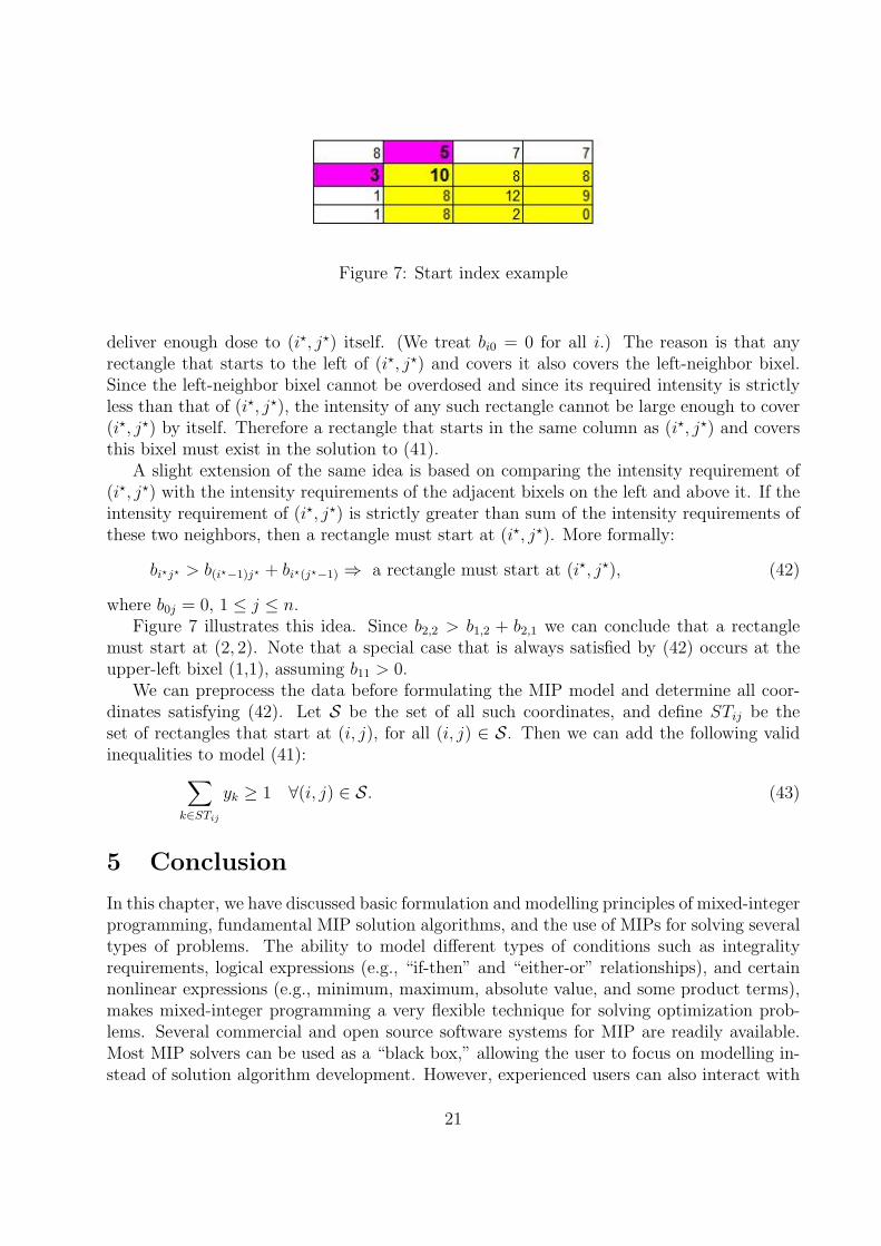
Figure 7: Start index example

deliver enough dose to (i?, j?) itself. (We treat bi0 = 0 for all i.) The reason is that anyrectangle that starts to the left of (i?, j?) and covers it also covers the left-neighbor bixel.Since the left-neighbor bixel cannot be overdosed and since its required intensity is strictlyless than that of (i?, j?), the intensity of any such rectangle cannot be large enough to cover(i?, j?) by itself. Therefore a rectangle that starts in the same column as (i?, j?) and coversthis bixel must exist in the solution to (41).

A slight extension of the same idea is based on comparing the intensity requirement of(i?, j?) with the intensity requirements of the adjacent bixels on the left and above it. If theintensity requirement of (i?, j?) is strictly greater than sum of the intensity requirements ofthese two neighbors, then a rectangle must start at (i?, j?). More formally:

bi?j? > b(i?−1)j? + bi?(j?−1) ⇒ a rectangle must start at (i?, j?), (42)

where b0j = 0, 1 ≤ j ≤ n.Figure 7 illustrates this idea. Since b2,2 > b1,2 + b2,1 we can conclude that a rectangle

must start at (2, 2). Note that a special case that is always satisfied by (42) occurs at theupper-left bixel (1,1), assuming b11 > 0.

We can preprocess the data before formulating the MIP model and determine all coor-dinates satisfying (42). Let S be the set of all such coordinates, and define STij be theset of rectangles that start at (i, j), for all (i, j) ∈ S. Then we can add the following validinequalities to model (41):∑

k∈STij

yk ≥ 1 ∀(i, j) ∈ S. (43)

5 Conclusion

In this chapter, we have discussed basic formulation and modelling principles of mixed-integerprogramming, fundamental MIP solution algorithms, and the use of MIPs for solving severaltypes of problems. The ability to model different types of conditions such as integralityrequirements, logical expressions (e.g., “if-then” and “either-or” relationships), and certainnonlinear expressions (e.g., minimum, maximum, absolute value, and some product terms),makes mixed-integer programming a very flexible technique for solving optimization prob-lems. Several commercial and open source software systems for MIP are readily available.Most MIP solvers can be used as a “black box,” allowing the user to focus on modelling in-stead of solution algorithm development. However, experienced users can also interact with

21

the solver using general-purpose programming languages such as C, C++, Java, C#, andVisual Basic. This flexibility allows users to guide the solution algorithm in order to exploitspecial structures of the problem on hand, resulting in more efficient solver performance.

Even though MIP models are designed to find a provably optimal solution, it is possibleto stop execution once a “good enough” solution is found. In other words, it is possible to useMIP-based algorithms as heuristics in computationally difficult problems. However, thereis an important distinction between problem specific heuristics and MIP-based algorithms:unlike the former, MIP-based algorithms are capable of measuring the quality of the solutionfound with respect to the (unknown) optimal solution. These features make mixed-integerprogramming a suitable technique for solving difficult optimization problems, including thosein healthcare applications.

References

[1] M. S. Bazaraa, J. J. Jarvis, and H. D. Sherali. Linear Programming and Network Flows.John Wiley & Sons, New York, second edition, 1990.

[2] G. Bednarz, D. Michalski, C. Houser, M. S. Huq, Y. Xiao, P. R. Anne, and J. M. Galvin.The use of mixed-integer programming for inverse treatment planning with pre-definedfield segments. Physics in Medicine and Biology, 47(13):2235–2245, 2002.

[3] J. Deasy, E. K. Lee, T. Bortfeld, M. Langer, K. Zakarian, J. Alaly, Y. Zhang, H. Liu,R. Mohan, R. Ahuja, A. Pollack, J. Purdy, and R. Rardin. A collaboratory for radia-tion therapy treatment planning optimization research. Annals of Operations Research,148(1):55–63, 2006.

[4] M. Elshafei, H. D. Sherali, and J. C. Smith. Radar pulse interleaving for multi-targettracking. Naval Research Logistics, 51(4):72–94, 2004.

[5] K. Engel. A new algorithm for optimal multileaf collimator field segmentation. DiscreteApplied Mathematics, 152:35–51, 2005.

[6] A. Farina and P. Neri. Multitarget interleaved tracking for phased-array radar. IEEEProceedings, Part F: Communications, Radar & Signal Processing, 127(4):312–318,1980.

[7] M. Ferris, R. Meyer, and W. D’Souza. Radiation treatment planning: Mixed inte-ger programming formulations and approaches. In G. Appa, L. Pitsoulis, and H. P.Williams, editors, Handbook on Modelling for Discrete Optimization, volume 88, pages317–340. Springer, New York, NY, 2006.

[8] F. S. Hillier and G. J. Lieberman. Introduction to Operations Research. McGraw-Hill,New York, NY, eighth edition, 2005.

[9] E. K. Lee, T. Fox, and I. Crocker. Integer programming applied to intensity-modulatedradiation therapy treatment planning. Annals of Operations Research, 119:165–181,2003.

22

[10] G. L. Lim, J. Choi, and R. Mohan. Iterative solution methods for beam angle andfluence map optimization in intensity modulated radiation therapy planning. TechnicalReport 10-01, Department of Industrial Engineering, University of Houston, Houston,TX, 2006.

[11] G. L. Nemhauser and L. A. Wolsey. Integer and Combinatorial Optimization. JohnWiley & Sons, New York, NY, 1999.

[12] F. Preciado-Walters, R. Rardin, M. Langer, and V. Thai. A coupled column generation,mixed integer approach to optimal planning of intensity modulated radiation therapyfor cancer. Mathematical Programming, 101(2):319–338, 2004.

[13] H. E. Romeijn, R. K. Ahuja, J. F. Dempsey, and A. Kumar. A column generationapproach to radiation therapy treatment planning using aperture modulation. SIAMJournal on Optimization, 15(3):838–862, 2005.

[14] H. E. Romeijn, R. K. Ahuja, J. F. Dempsey, A. Kumar, and J. G. Li. A novel linearprogramming approach to fluence map optimization for intensity modulated radiationtherapy treatment planning. Physics in Medicine and Biology, 48(21):3521–3542, 2003.

[15] A. Schrijver. Theory of Linear and Integer Programming. John Wiley & Sons, NewYork, NY, 1986.

[16] H. D. Sherali and J. C. Smith. Interleaving two-phased jobs on a single machine withapplication to radar pulse interleaving. Discrete Optimization, 2(4):348–361, 2005.

[17] W. L. Winston and M. Venkataramanan. Introduction to Mathematical Programming:Applications and Algorithms, Volume 1. Duxbury Press, Belmont, CA, fourth edition,2002.

[18] L. A. Wolsey. Integer Programming. John Wiley & Sons, New York, NY, 1998.

23