A Tractable Monetary Model under General Preferences

TSZ-NGA WONG∗

The Bank of Canada

First version received November 2013; final version accepted June 2015 (Eds.)

Abstract

This paper studies an economy with both centralised and decentralised monetary ex-

changes under search frictions. A degenerate asset distribution is featured under a broad

class of preferences including, for example, constant return to scale, constant elasticity of

substitution, CARA and others from a range of macroeconomic literatures. Some novel

applications impossible under quasi-linear preferences, for example endogenous growth,

are illustrated under this class of preferences. This paper finds that the welfare cost and

growth loss of inflation can be much higher in these applications than previous estimates.

Keywords: Money, Search and Matching, Bargaining and General Trading Protocols,

Endogenous Growth, Heterogeneous-Agent Model.

∗Acknowledgement. For their helpful comments, I thank Gabriele Camera, Jonathan Chiu, Tai-Wai Hu,Ricardo Lagos, Miguel Molico, Daniel Sanches, Enchuan Shao, Eric Swanson, Steve Williamson, and espe-cially Guillaume Rocheteau and Randy Wright, as well as the participants of the Money, Banking, Paymentand Finance Workshop 2013 at the Federal Reserve Bank of Chicago, the Midwest Theory Meeting 2013 atMichigan State Univerity as well as the seminars at the Bank of Canada and UC Irvine for comments. I alsothank three anonymous referees for very helpful suggestions. I am deeply grateful for comments from theeditor Phillipp Kircher and one referee, which substantially improved this paper. The views expressed in thepaper are mine and nothing should be attributed to the Bank of Canada.

1 Introduction

In their seminal work, Lagos and Wright (2005, henceforth LW) devise a monetary model

with uninsurable risks of decentralised trades that features a degenerate distribution of money

holding in the equilibrium.1 The degeneracy makes keeping track of distribution manageable

in a dynamic economy; otherwise the analysis can be challenging as in the incomplete markets

literature. Two key features in LW are to allow agents to trade in centralised markets between

decentralised trades, and to assume quasi-linear preferences in those centralised markets.

This paper generalises LW’s results to a broad class of preferences without quasi-linearity.

This class of preferences includes the Stone-Geary utility, Greenwood—Hercowitz—Huffman

utility, and utility functions with features like constant return to scale, constant elasticity of

substitution (and hence Cobb-Douglas), CARA, quasi-linearity certainly, and many others.

With this class of preferences, the history of money holdings does not affect the optimal money

holding; nevertheless it is affected by preferences, technology and policy. Such a feature allows

endogenous, degenerate distribution of money holding in the simple setting without ex-ante

heterogeneity; and even with large ex-ante heterogeneity it allows a non-degenerate but still

tractable distribution.

But, beyond the technical contribution, why generalise the preferences? Of course, it

never hurts to work with a broader class of preferences. Yet a more important argument is

that the quasi-linearity assumption undermines some of LW’s intended advantages. On one

hand the introduction of centralised markets taps into the potential of connecting a search

model of money to a significant body of macroeconomic literature; however, on the other

hand, the quasi-linearity assumption can be too restrictive for relevant macroeconomic ap-

plications. One important example of this conflict can be found when applying LW to study

inflation and endogenous growth. In Section 5 I show that incorporating the standard endoge-

nous growth model of Lucas (1988) in LW fails to generate endogenous growth, essentially

because of the absence of curvature under the quasi-linear preferences. Instead, formulating

endogenous growth with this class of preferences can easily capture a growth mechanism of

inflation, which is also consistent with data. This example makes the point that the general-

isation of preferences offers the capacity to model applications impossible under quasi-linear

preferences. It also illustrates that these new applications of LW can have important policy

1See Lagos, Rocheteau and Wright (2014) for a recent survey. Also see Shi (1997) for an alternative "bighousehold" approach, where the trading risks of members are pooled within the household. See Lagos andWright (2005) for a comparison of the two approaches.

1

implications. For instance, when growth is endogenous, inflation has a larger impact on wel-

fare because not only is current output affected, but also the entire path of future output. In

sum, generalising preferences helps open up a wide new possibility of applications leading to

a very different understanding of policies, without compromising tractability.

The generalisation does not only widen the scope of the search models of money, but

also other macroeconomic literatures. Going back to the previous example, it introduces

to the endogenous growth literature new features such as search, bargaining and various

trading protocols; novel mechanisms such as the strategic complementarity between buyers

and sellers; and additional sources of ineffi ciency such as the two-sided hold-up problem.

While these are impossible under the standard paradigm of Walrasian markets, their synthesis

is now possible with the search models since this class of preferences has been used in many

areas of macroeconomics; see Section 4 for a survey.

While in this paper I only focus on the monetary models, in a broader sense, in any

intertemporal model with heterogeneity inserting a subperiod with this class of preferences

will lead to a tractable wealth distribution - an analytical environment not commonly found

in the literature.2 Section 6 elaborates this feature. Alternatively, while the numerical ap-

proach is also useful and complementary, it has less to say about properties such as existence,

uniqueness or multiplicity, and dynamics. A tractable model also provides a useful benchmark

to validate numerical methods. Furthermore, a tractable model makes heterogeneous-agent

models easily extendable to other applications, for example, even to the non-stationary en-

vironment with endogenous growth shown in Section 5. Finally, a tractable model helps

explain the economy, especially when several mechanisms come into effect, which are diffi cult

to single out from numerical examples.

2 Basic Model

Overview. The environment is the same as LW except this paper use more general prefer-

ences. Time is discrete and infinite, indexed by t = 0, 1... Alternating in each period are two

markets: a frictional decentralised market (DM) where agents match bilaterally and bargain,

2See Bewley (1980), Aiyagari (1994), and Buera and Shin (2013) for the challenge of distribution underincomplete markets. One can still proceed with the distribution directly but restricting the terms of tradeas well as the domain and divisibility of assets, as in Kiyotaki and Wright (1989) and Trejos and Wright(1995). Or one can apply numerical methods "approximating" the equilibrium distribution like Krusell andSmith (1996), Molico (2006) and Chiu amd Molico (2010). Also see Menzio, Shi and Sun (2013) for a directedsearch approach for a relatively tractable computational model that produces non-degenerate distribution.See Rocheteau, Weill and Wong (2015) for a distribution model formulated in the continuous time.

2

and a frictionless centralised market (CM) where agents trade with each other at Walrasian

prices. In the DM agents can only observe the actions and outcomes of their trades, and are

anonymous. There is no technology for recordkeeping, commitment or coordinating global

punishment. As a result, debt contract is infeasible and a medium of exchange - money -

is essential for trades in the DM.3 Money supply grows exogenously, Mt+1 = (1 + τ)Mt,

by lump-sum transfers to agents in the CM. Let φ be the price of money in terms of the

CM goods (numeraire). There can be inflation in this economy; denote the inflation rate as

πt ≡ φt/φt+1 − 1. As seen later, the real balances z ≡ φm is the relevant state variable for

agent’s decision.

Technology and preference. A unit measure of agents live forever with a discount

factor β ∈ (0, 1). Utility in a period involves actions in the CM and DM. In the CM, agents

consume the numeraire goods X, where the production function is AH using labour H; in

the DM, agents consume a different goods x, produced one-to-one with the DM labour q.

The following form of utility function is maintained throughout this paper:

U (X,H, x, q) = u (x)− c (q) + U(X,H −H

),

where H is the maximal H an agent can work. The agent’s lifetime preferences are given by

E∑βtU (Xt, Ht, xt, qt). The following standard assumptions are thus made:4

Assumption 1 (Smoothness) U ∈ C2 and u ∈ C2, where UXX < 0, UHH ≤ 0, UXH ≤ 0,

ux > 0, uxx < 0, cq > 0, cqq ≥ 0 and u satisfies the Inada condition. Also, u (0) =

c (0) = 0.

Assumption 2 (Large labour endowment) For any finite ω, there exists a unique so-

lution X > 0 and H ∈(0, H

)to maxX,H U

(X,H −H

)s.t. X = AH + ω, if H is

suffi ciently large.

The agent’s problem is as follows. Let Wt (s) and Vt (z) denote the value functions in the

CM and DM with real balances s and z respectively. The CM problem is

Wt (s) = maxX,H,z

{U(X,H −H

)+ βVt+1 (z)

}, (1)

3See Kocherlakota (1998) for the role of recordkeeping, and Wallace (2010) for details on the essentialityof money. The DM is a useful modelling device to capture all these frictions.

4Assumption 1 guarantees that the economy is "smooth", and there exist some trades in the DM witha positive social surplus (otherwise no trade in the DM is preferable). Assumption 2 guarantees an interiorsolution in the equilibrium. Both assumptions are satisfied in Lagos and Wright (2005). For simplicity I donot consider any upper bound for q.

3

s.t. X = AH + s− (1 + πt+1) z + Tt, (2)

X ≥ 0, H ∈[0, H

], z ≥ 0, (3)

where (2) is the agent’s budget constraint, (3) are boundary constraints, Tt is the lump sum

injection (drain if negative) of money from the government, and the inflation factor 1+πt+1 =

φt/φt+1 captures changes in the real prices across periods. Let Xt (s), Ht (s) and zt (s) denote

the solutions to (1) given s units of real balances and the DM value function Vt+1 (z). The

Bellman equation for Vt+1 (z) is given below. The solution {Xt (s) , Ht (s) , zt (s)} to (1) is

interior if the boundary constraints (3) are slack.

Decentralised trades. Now I turn to the heart of the double-coincidence problem in

the DM that gives rise to monetary exchange. Some agents (sellers) can produce but do not

want to consume, while others (buyers) want to consume but cannot produce, and hence

trades emerge. In the DM, with probability α ≤ 1/2, the agent matches and buys x from a

seller with payoff u (x). By symmetry, there is also probability α that the agent matches and

sells q to a buyer with cost c (q).

Suppose the real balances held by the buyer and seller are z and z′ respectively. In a

bilateral match in the DM, the seller’s sales q must equal the buyer’s purchase x. Denote

their common value as q (z, z′,Wt), and the real balances that change hands to the seller

by d (z, z′,Wt), which in general depends on the real balances and the continuation value.

Denote the buyer’s surplus and seller’s surplus as

Sb(z, z′,Wt

)≡ u

[q(z, z′,Wt

)]+Wt

[z − d

(z, z′,Wt

)]−Wt (z) ,

Ss(z, z′,Wt

)≡ −c

[q(z, z′,Wt

)]+Wt

[z′ + d

(z, z′,Wt

)]−Wt

(z′).

At the beginning of DM, given real balances z, the agent’s value function Vt (z) is given by

the following Bellman equation

Vt (z) = α

∫Sb(z, z′,Wt

)dFt

(z′)

+ α

∫Ss(z′, z,Wt

)dFt

(z′)

+Wt (z) , (4)

where Ft (z) is the distribution of z in the beginning of the DM. There is probability density

αdFt (z′) that an agent meets a seller (buyer) with real balances z′ in the DM and results in the

buyer surplus Sb (z, z′,Wt) [seller surplus Ss (z′, z,Wt)]. Thus, Sb (z, z′,Wt) and Ss (z, z′,Wt)

summarize the essential information about the trading protocols {q (z, z′,Wt) , d (z, z′,Wt)}

for agents to choose their money holdings.

4

Trading protocols. Without loss of generality, I take the surplus functions Sb (z, z′,Wt)

and Ss (z, z′,Wt) as primitives, since the mappings only depend on the exogenous trading

protocol {q (·) , d (·)} rather than any endogenous variable. This formulation effectively covers

any trading protocol without going into details. For example, consider the trading protocol

{q (z, z′,Wt) , d (z, z′,Wt)} that solves the Nash bargaining problem:

maxq,d

(Sb)θ

(Ss)1−θ s.t. (5)

Sb = u (q) +Wt (z − d)−Wt (z) ,

Ss = −c (q) +Wt

(z′ + d

)−Wt

(z′),

d ∈[−z′, z

].

The buyer’s bargaining power is given by θ ∈ (0, 1]. The Nash bargaining problem can be

suffi ciently represented by the corresponding Sb (z, z′,Wt) and Ss (z, z′,Wt) to (5). In general,

I maintain the following assumption on Sb (z, z′,Wt) and Ss (z, z′,Wt).5

Assumption 3 (Trading protocol) For any z, z′ > 0 and j = b, s,

(i) Sj (z, z′,W ) is upper semi-continuous in z and z′, Sj (z, z′,W ) ≥ 0 and Sb1 (0+, z′,W ) +

Ss2 (z′, 0+,W ) > 1+τ−βαβ W1 (0+);

(ii) Sj (z, z′,W ) = Sj (z, z′,W + w0) for any finite w0.

(iii) There exists z <∞ such that Sb (z, z′,W ) ≤ Sb (z, z′,W ) and Ss (z′, z,W ) ≤ Ss (z′, z,W )

for any z ≥ z and z′ ≥ 0.

Assumption 3 is weak and natural; it is satisfied under protocols like Nash bargaining,

proportional bargaining, random ultimatum (illustrated in the later sections), competitive

pricing, pairwise core and many others.6

Equilibrium. The law of motions of the individual real balances st and zt depends on5Gu, Mattesini and Wright (2014) also propose a general trading protocol based on a tighter structure

of axioms. Assumption 3 is tailored to establish the proof of degeneracy in this economy. Assumption 3iguarantees the solution to the DM trades exists, which involves a positive payment; Assumption 3ii states thata "parallel shift" to the continuation value does not change the trading protocol; Assumption 3iii guaranteesinifinite money holding is never optimal.

6Notice that with the generalized Nash bargaining Sb (z, z′,W ) may not increase in z; with the propor-tional bargaining Sb1 (0, z

′,W ) is bounded even though ux (0) = ∞; with random ultimatum q (z, z′,W ) andd (z, z′,W ) can be stochastic; and with pairwise core Sb (z, z′,W ) may not be continuous. These are allowedin my formulation of the general trading protocol.

5

the trading protocol, which is given by

st =

z − d (z, z′,Wt) with density αdFt (z′) ,

z + d (z′, z,Wt) with density αdFt (z′) ,

z with probability 1− 2α,

(6)

zt+1 = zt (s) , where s follows Gt (s) , (7)

where Gt (s) is the distribution of s according to (6) and Ft+1 (z) is the distribution of z

according to (7). Suppose F0 is degenerate at z = φ0M0. Define a (monetary) equilibrium:

Definition 1 An equilibrium consists of positive real prices {φt}∞t=0, allocation {Xt, Ht, zt, qt, dt}∞t=0and distributions {Ft, Gt}∞t=0 such that

(i. agent optimization) For any s ∈ dom (Gt), {Xt (s) , Ht (s) , zt (s)} solves the agent’s

optimization problem (1), and {Wt (s) , Vt (z)} solves the Bellman equations (1) and (4);

(ii. bargaining) qt = q (z, z′,Wt) and dt = d (z, z′,Wt) for any z, z′ ∈ dom (Ft);

(iii. goods markets clear)∫Xt (s) dGt (s) = A

∫Ht (s) dGt (s);

(iv. money markets clear)∫zt (s) dGt (s) = φt+1Mt+1;

(v. government budget) Tt = τφtMt;

(vi. law of motion) Gt (s) and Ft (z) are given by (6) and (7).

A degenerate (and stationary monetary) equilibrium is an equilibrium that also satisfies

zt (s) = z∗ for all s ∈ dom (Gt), i.e., all agents always exit the CM with the same real balances,

regardless of the ones they enter the CM. In general, there can be degenerate equilibria that

are, for example, non-monetary, non-stationary, cyclic, chaotic or driven by sunspots; they

are not analysed in this paper.7

3 Main Results

I now specify a general environment that admits a degenerate equilibrium. To ease the

presentation, I first digress to introduce an assumption on preferences and then verify the

degenerate equilibrium.

Assumption 4 (General preferences) U ∈ C2 satisfies

UXXUHH − (UXH)2 = 0. (8)

7These examples of equilibria can be found in Lagos and Wright (2003).

6

I refer the set U ⊆ C2 as the collection of utility functions U satisfying (8). Obviously, the

quasi-linear preferences in LW satisfy Assumption 3 with UHH = UXH = 0. An important

property of U is given by the following lemma:

Lemma 1 If UXX 6= 0, then U satisfies (8) if and only if there exists a function Λ ∈ C1 such

that UH = Λ ◦ UX .

Lemma 1 is helpful to give some sense about how degeneracy is possible. Suppose solutions

are interior and Vt+1 is differentiable. From the first order condition with respect to z in (1),

I have

(1 + π)UX,t = βVz,t+1.

Also, from the first order condition with respect to X in (1), I have the intertemporal Euler’s

equation:

AUX,t = −UH,t.

Combining these two equations with UH,t = Λ (UX,t) from Lemma 1, I have

βA

1 + π=

Λ[

β1+πVz,t+1 (z)

]Vz,t+1 (z)

.

Since the right side is a function of z only, not s, it implies zt (s) is a constant function

on the equilibrium path. Thus, the history of money holding does not affect the optimal

money holding. For example, it is straightforward to verify the non quasi-linear case U =

X1−σ (H −H)σ. In general Vt+1 might not be differentiable (for example, under the pairwise-core trading protocol used in Hu, Kennan and Wallace 2009) and the solutions might not

be interior, so a more sophisticated argument is needed to show the degenerate equilibrium,

summarized by the following proposition.

Proposition 1 If τ > β − 1 and H is suffi ciently large, then there exists a degenerate

equilibrium, which is unique for generic values of the other parameters.

Sketch of the proof. The strategy of proof is sketched as follows. I first establish

an auxiliary problem that agents choose X and H to maximize U in the CM, given st

and zt+1. It becomes a static problem and yields a value function in st and zt+1. One

complication is to check interior solutions under the general preferences. A key part of

the proof is that I transform the value function of the static problem as if it were some

7

quasi-linear utilities in the CM. I formulate a new problem in an auxiliary economy with

this quasi-linear utility in the CM, and keep everything in the DM unchanged. I show that

the solutions in the auxiliary economy are interior, and the value functions are the fixed

point of a contraction mapping from a space of linear functions into itself. This step is

done without relying on the differentiability of Vt in the original economy. Finally, I show

the existence and uniqueness of the degenerate equilibrium under the auxiliary economy. I

translate the equilibrium allocation of the auxiliary economy back to an allocation in the

original economy, which is also degenerate and satisfies all the equilibrium conditions of the

original economy under the same supporting prices and laws of motion. By construction,

the translated allocation also maximizes the agent’s preferences under the original economy.

Hence, the translated allocation constitutes a degenerate equilibrium.

Proposition 1 states that agents always exit the CM with the same real balances regardless

of the real balances entering the CM. The intuition is as follows. Consider the agent has

purchases in the DM, so some of the real balances s brought to the CM are depleted. Then,

due to the wealth effect, the agent wants to reduce his consumption X and increase his labour

supply H. If the labour endowment H is suffi ciently large, then X is also large enough to

buffer any reduction in X from the zero lower bound, and the increase in labour supply is

not restricted by H. As a result, the decrease in X and increase in H completely "rebalance"

the falling short of real balances s after the DM purchases. With quasi-linear preferences,

agents only rebalance the depleted real balances by increasing his labour supply H. With

the general preferences, it can also be rebalanced by reducing his consumption X as well.

The conditions of τ > β − 1 and a suffi ciently large H are common in the literature:

τ > β − 1 guarantees the return of money is not too high otherwise money is hoarded rather

than circulating; a suffi ciently large H guarantees an interior allocation. The uniqueness

holds for generic parameter space since there may be multiple degenerate equilibria under

some special combination of parameters.8

4 Exact Solutions

To make use of the utility function U , it is useful to obtain exact solutions rather than in the

PDE form UXXUHH − (UXH)2 = 0. The following lemma solves for the exact solutions:

Lemma 2 (i) U satisfies (8) if it has one of the following two forms:

8See Wright (2010) for a related discussion.

8

a. U = (C1X + C2H + C3)ϕ(C4X+C5H+C6C1X+C2H+C3

)+ C7X + C8H + C9;

b. U = (C1X + C2H)ϕ(XH

)+ C3X + C4H + C5,

where Ci, i = 1...9, are arbitrary constants and ϕ ∈ C2.

(ii) U satisfies (8) if and only if it has the following parametric form:

U = pX + Λ (p)H + χ (p), where p solves −χ′ (p) = X + Λ′ (p)H, Λ ∈ C1 and χ ∈ C1.

Lemma 2 includes some utilities, such as the class of constant return to scale (CRS) pref-

erences, that have been extensively studied in many macroeconomic literatures. A popular

example of CRS is the utility with constant elasticity of substitution (CES), which has the

form U =[(1− σ)Xψ + σ

(H −H

)ψ]1/ψ, for all σ ∈ (0, 1) and ψ ∈ (−∞, 1). A Cobb-

Douglas utility U = X1−σ (H −N −H)σ is widely used to study endogenous growth withleisure, which will be illustrated in the next section. Heckman (1976) uses the CRS util-

ity U[X,A

(H −N −H

)]to capture the effective leisure A

(H −N −H

)on endogenous

growth. Barro and Becker (1989) use the CRS utility U = HU0(XH

), where U0 is some

increasing and strictly concave function, to study fertility by interpreting H as the size of a

family.

The utility class U also includes non-CRS functions. A prime example is the quasi-linear

utility U = U (X)−H used in LW. Another form of the quasi-linear utility U = X − g (H),

where g is an increasing convex function, is a special case of Greenwood—Hercowitz—Huffman

(GHH) utility, commonly used in international economics and business cycles when it is

desirable not to have any income effect in the labour supply curve w = gH (H). Another

non-CRS preference is the Stone-Geary utility U = (X − x0)1−σ(H −H

)σ, used extensively

in studies of international trade and structural change. Here, x0 is the level of subsistence

consumption. Other examples include the constant-absolute-risk-aversion (CARA) utility

U = − exp[−αXX − αH

(H −H

)]+α0X, where α0 > 0 can be arbitrarily small just to rule

out a bang-bang solution. CARA is widely used in, for example, the literatures of both asset

pricing and incomplete markets, since the associated consumption function is tractable even

in a stochastic environment. Some applications using these utility functions are illustrated

in the following sections.

5 Application to Endogenous Growth

In this section I illustrate how to make use of the general preferences to incorporate the stan-

dard endogenous growth model à la Lucas (1988) in a decentralised economy of monetary

9

exchange. This application also highlights the aspects where the generalisation of preferences

matters, qualitatively and quantitatively. Last but not least, it demonstrates how to incor-

porate particular bargaining protocols even when deviating from a stationary environment.

Engine of long-run growth. The basic environment is extended as follows. Agents

trade in the CM and DM as before, but now agents can also invest some time N in the CM

to improve their human capital A, which evolves according to the following law of motion:

At+1 = δ (Nt)At, (9)

where δ (N) is positive, increasing and strictly concave, and satisfies the Inada condition.

In the growing economy, the relevant individual states are human capital and real balances,

which are denoted as aD = (A, z) in the beginning of the DM and aC = (A, s) in the

beginning of the CM. Compared with the literature, Lucas (1988) is the special case without

decentralised markets, and Lagos and Wright (2005) is the special case with δ (N) = 1.

Bargaining protocol. To illustrate as well as to simplify the environment, I assume a

random ultimatum game in the DM: there is probability θ (probability 1− θ) that the buyer

(seller) can make a take-it-or-leave-it offer.9 Similar to Nash and proportional bargaining

alike, θ ∈ (0, 1] captures the buyer’s bargaining power. When a buyer of state a = (A, z) can

make an offer to a seller of state a′ = (A′, z′), he will propose the offer [qb (a,a′) , db (a,a′)]

that maximizes his continuation value subject to the seller’s participation constraint:

maxqb,db∈[−z′,z]

{u (qb) +W (A, z − db)} s.t. W(A′, z′

)= −c (qb) +W

(A′, z′ + db

). (10)

On the other hand, when a seller of state a′ can make an offer, his proposal [qs (a,a′) , ds (a,a′)]

is given by

maxqs,ds∈[−z′,z]

{−c (qs) +W

(A′, z′ + ds

)}s.t. W (A, z) = u (qs) +W (A, z − ds) . (11)

I first hypothesize, and then verify, that the equilibrium is degenerate, i.e. the individual

states for the rest of the agents is a′. By summarizing all the cases, the (ex-ante) DM value

9Under other bargaining protocols, agents may also want to accumulate human capital in order to improvetheir bargaining solution when they turn out to be buyers. However, assuming a random ultimatum simplifiesthe economy by shutting down this interesting channel.

10

function V (a) is given by the following Bellman equation:

V (a) = αθ{u[qb(a, a′

)]+W

[a1,a2 + db

(a, a′

)]}(12)

+α (1− θ){−c[qs(a′,a

)]+W

[a1,a2 + ds

(a′,a

)]}+ (1− α)W (a) .

The first (second) term is the ex-post DM value if the agent can match and make a offer to

a seller (buyer), which happens with probability αθ [probability α (1− θ)]. When the agent

cannot match anyone in the DM, or can match someone but cannot propose, which happens

with probability 1 − α, the ex-post DM value is simply W (a), given the result that the

participation constrains in (10) and (11) are always binding. Moving to the next subperiod,

the CM value function W (A, z) is given by the following Bellman equation:

W (A, s) = maxX,H,N,z

{U(X,H −H −N

)+ βV [δ (N)A, z]

}, s.t. (13)

X = AH + s− (1 + π) z + T,

X ≥ 0, N ∈[0, H

], H ∈

[0, H −N

], z ≥ 0.

Denote{X(aCt), H(aCt), N(aCt), z(aCt)}the solution to (13), which can be growing un-

bounded following aCt .

Equilibrium.10 Define a degenerate balanced growth path as follows: a degenerate

equilibrium such that z(aCt)/At = z∗ and N

(aCt)

= N∗ for any aCt on the equilibrium

path; as well as the CM and DM outputs,∫AtH

(aCt)dGt

(aCt), qb,t and qs,t, all grow at

the same factor δ (N∗). Notice that, unlike the static economy, on the degenerate balanced

growth path inflation is given by 1+π = (1 + τ) δ (N∗)−1; inflation and money growth are no

longer the same. Without loss of generality, I assume that the government sets τ as passive

to directly target π in the equilibrium; hence π is treated as an exogenous policy variable.

General preferences. So far I have abstracted from any specification of preferences.

Following Lucas (1988), I assume that the CM utility is given by the following member of U :

U(X,H −H −N

)= B

(X

1− σ

)1−σ (H −H −Nσ

)σ, σ ∈ (0, 1) , (14)

where B > 0 is the weight of the CM utility. I also use general CRRA functions for the

10Here I assume that Bellman equations are valid under unbounded growth. See Alvarez and Stokey (1998).However, Bellman equations may no longer be valid when utility is not bounded, for example, for a log utilityfunction. As seen later, the utilities given by (14), (15) and (16) are homogenous of degree 1−σ. Nevertheless,the suffi cient conditions given in Alvarez and Stokey (1996) are indeed satisfied under the general preferences.

11

preferences in the DM, which are given by

u (q) = Dq1−γ

1− γ , γ ∈ [0, 1] , (15)

c (q) =q1+ηA−ϕ

ϕ, η, ϕ ≥ 0, (16)

where D > 0 is the weight of the DM consumption. The case γ = 1 is interpreted as log

utility as usual. All parameters are to be estimated in the later quantitative exercise. Before

that, however, I need the following proposition to show the conditions for the existence of a

degenerate balanced growth path with the utility function (14).

Proposition 2 (Existence under General Preferences) Given the utility function of

form (14), a degenerate balanced growth path exists if π ≥ β [maxN δ (N)]−σ − 1, H is suffi -

ciently large, and the parameters satisfy

γ = σ, (17)

ϕ = σ + η. (18)

Condition (17) [(18)] guarantees a degenerate balanced growth path in the DM when the

seller (buyer) proposes. The condition of a large labour endowment H guarantees an interior

solution, as before. The condition π ≥ β [maxN δ (N)]−σ − 1 is the growth version of the

standard condition π > β − 1: the return of money −π cannot be too high to be used as a

medium of exchange in the DM.

What happens if (14) is replaced with the quasi-linear preferences U (X) −H − N in a

growing economy? As Waller (2011) finds but with other bargaining protocols, the existence

of a balanced growth path under the quasi-linear preference requires extra conditions.11

Proposition 3 (Waller 2011) If quasi-linear preferences are assumed, then the necessary

conditions for the existence of a degenerate balanced growth path include: (a) U (X) = logX,

(b) θ = γ = 1 and (c) ϕ = 1 + η.

Compared with the general preferences, under the quasi-linear preferences conditions (a)

and (b) in Proposition 3 are the extra conditions for the existence of a degenerate balanced

growth path. The intuition is as follows. The intratemporal Euler’s equation under the11For readers familiar with the literature, condition (a) is necessary for a balanced growth path in the CM,

and condition (b) is necessary for a balanced growth path in the DM, which is not considered in Waller (2011).Also, he restricts η = 0.

12

quasi-linear preferences requires UX (X) = A−1. To have both sides of equality grow at

the same rate, log utility is necessary. Instead, under the general preferences, both labour

and consumption can be used to satisfy UX = −A−1UH , so there is a larger degree of

freedom for parameters. Second, log utility also means that the shadow value of real balances,

UXz = z/A, is constant on the balanced growth path, so the DM goods traded in the

decentralised markets are also constant when sellers can make offers. To have consumption

growth in the decentralised markets, any chance that sellers can propose must be shut down,

by restricting the economy such that buyers have all the bargaining power, θ = 1. In sum, a

quasi-linear economy needs extra conditions to maintain a knife-edge growth path.

The following proposition gives an implication of these restrictions: in a quasi-linear

economy inflation does not affect the output growth rate.

Proposition 4 (No Endogenous Growth under QL) On any degenerate balanced growth

path under quasi-linear preferences, δ (N∗) solves δ (N∗) = βδ′ (N∗).

Under the quasi-linear preferences, the output growth does not depend on inflation. To

see this, recall that in the Lucas model the growth rate is endogenously chosen to balance the

opportunity cost and benefit of accumulating human capital. With quasi-linear preferences,

the cost is independent to inflation as the marginal disutility of labour supply is constant.

Also, agents no longer have any benefit from investing human capital for the DM production

since sellers have no bargaining power (necessary for the balanced growth under quasi-linear

preferences). Thus, a quasi-linear economy essentially shuts down any potential mechanism

that inflation can affect growth. Of course, the absence of the growth mechanism is no longer

the case under the general preferences. The following proposition summarizes the key result

in this section:

Proposition 5 (Growth Mechanism under General Preferences) Given the utility

function of the form (14), on the degenerate balanced growth path, the comparative statics are

given by dz∗/dπ < 0 and dδ (N∗) /dπ ≤ 0. The inequality is strict if the equilibrium features

z∗ < DB(1−γ)

(ϕD1+η

) 1−γη+γ.

A lesson from comparing Proposition 4 with Proposition 5 is that formulating an LW

model with the general preferences can feature this growth mechanism but is impossible

under the quasi-linear preferences. The growth mechanism under the general preferences

relates to the strategic complementarity between human capital and real balances. On one

13

hand, a lower level of a buyer’s real balances affords less purchases, and hence the seller

wants to invest less human capital to justify the lower level of production. On the other

hand, a lower level of a seller’s human capital worsens the buyer’s terms of trade, and hence

the buyer wants to hold less real balances. Since a higher inflation raises the shadow cost

of holding real balances, it reduces the investment in human capital through the strategic

complementarity, and eventually triggers a further cut in real balances holding, and so on.12

The strategic complementarity amplifies the negative effect of inflation.

It is also useful to notice a new source of ineffi ciency under the general preferences: this

economy features a two-sided hold-up problem. On average, only portion 1− θ (portion θ) of

the time can the sellers (buyers) get the entire ex-post trade surplus, but the sellers (buyers)

must bear the entire cost of investing in human capital (real balances) - a hold-up problem

for both sides of trade. Under the quasi-linear preference the economy is in the corner case

θ = 1: it reduces to a one-sided hold-up problem without strategic complementarity. The

welfare cost of inflation can be very different under the general preferences.

Preliminary quantitative finding. To give some sense of the inflation cost under the

general preferences, I perform a quantitative exercise closely following LW. This section serves

an illustrative purpose, due to the obvious diffi culty in assessing the relevance of inflation

for future output growth.13 The annual rate of time preference is r = β−1 − 1 = 0.04,

the matching rate is α = 0.5, and the buyer’s bargaining power is θ = 0.5. I normalize

H = 1 since existence is no longer a concern in the quantitative exercise. The remaining

parameters are estimated based on the same U.S. data from 1900 to 2000 used by Lucas

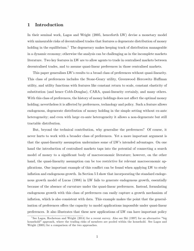
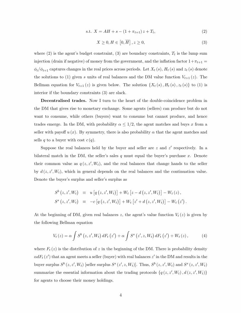
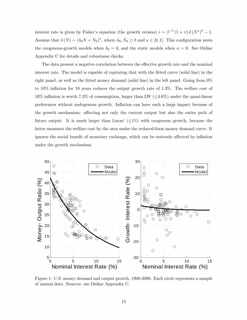
(2000), LW and many others. Figure 1 displays the plots of annual observations (the circles

in the figures) on the nominal interest rate i, on the money-output ratio L ≡ M/ (PY ),

and on the growth-interest rate differential ρ ≡ P+1Y+1PY (1 + i)−1 − 1. The data on L and ρ

capture the money demand and effective growth rate respectively. In the model the nominal

12Sellers can propose DM trades at the constrained effi cient level (condition on A) when the buyers holdhigher real balances than the threshold in Proposition 5. In this case a higher inflation does not affect seller’ssurplus or the incentive to invest human capital.13Some features of the model may result in overstating the welfare cost. First, as in the Lucas (1988) model,

agents can invest in human capital with their labour in every period. In practice, while human capital canbe accumulated by a continuous learning process (e.g. through experience and skill), a significant share ofhuman capital is formed at the early stage of the life cycle and at much lower frequency than in the model.Second, I estimate the model with the data of output growth rate rather than some direct observation onhuman capital such as years and quality of schooling. While it avoids taking a stance on what human capitalreally is and how to measure properly, still an ongoing issue in the growth literature, my empirical exercisedoes not directly verify the mechanism with the micro data. In particular, the negative effect of inflation onhuman capital accumulation suggested by the aggregate data might be weaker in the micro data. Last butnot least, money is the only medium of exchange. Further research will be required.

14

interest rate is given by Fisher’s equation (the growth version) i = β−1 (1 + π) δ (N∗)σ − 1.

Assume that δ (N) = (δ0N +N0)κ, where δ0, N0 ≥ 0 and κ ∈ [0, 1]. This configuration nests

the exogenous-growth models when δ0 = 0, and the static models when κ = 0. See Online

Appendix C for details and robustness checks.

The data present a negative correlation between the effective growth rate and the nominal

interest rate. The model is capable of capturing that with the fitted curve (solid line) in the

right panel, as well as the fitted money demand (solid line) in the left panel. Going from 0%

to 10% inflation for 10 years reduces the output growth rate of 1.3%. The welfare cost of

10% inflation is worth 7.3% of consumption, larger than LW (≤4.6%) under the quasi-linear

preferences without endogenous growth. Inflation can have such a large impact because of

the growth mechanism: affecting not only the current output but also the entire path of

future output. It is much larger than Lucas’ (≤1%) with exogenous growth, because the

latter measures the welfare cost by the area under the reduced-form money demand curve. It

ignores the social benefit of monetary exchange, which can be seriously affected by inflation

under the growth mechanism.

0 5 10 155

10

15

20

25

30

35

40

45

50

Nominal Interest Rate (%)

Mon

ey­ O

utpu

t Rat

io (%

)

DataModel

0 5 10 15­30

­20

­10

0

10

20

30

Nominal Interest Rate (%)

Gro

wth

­ In

tere

st R

ate 

(%)

DataModel

Figure 1: U.S. money demand and output growth, 1900-2000. Each circle represents a sampleof annual data. Sources: see Online Appendix C.

15

6 Application to a Heterogeneous-Agent Economy

The main insight of this paper is that under the general preferences the optimal money

holdings for the future periods are not a function of how much money they obtained in

the past. Proposition 1 concludes that ex-ante homogeneous agents hold identical amounts

of money. But the basic insight is broader. Even when agents are ex-ante heterogeneous,

the amount of money they want to take into the future does not depend on money earned

in previous trades; nevertheless it is affected by ex-ante heterogeneity in preferences and

productivities. In such environments, allowing general utility functions rather than restricting

attention only to quasi-linear utilities generates some advantages that this section will outline.

I introduce ex-ante heterogeneity as in standard incomplete-market models but keep the

changes to the benchmark model minimal. In this case, money holding is similar to capi-

tal in the incomplete-market models. Under a suffi ciently large ex-ante heterogeneity, the

distribution may cease to be tractable under the quasi-linear preferences. This section thus

provides another example to illustrate some advantages of modeling with this class of general

preferences: an economy can still feature a tractable distribution under a suffi ciently large

ex-ante heterogeneity, which helps to obtain some useful results analytically. Again, it is for

illustrational purpose; there are ongoing researches with more thorough examination.14

Compared to the benchmark case in Section 2, in this economy agents are subject to

uninsurable i.i.d. shocks to A over time, which are realized at the beginning of the CM.15

The CM value function is given by

W (A, s) = maxX,H,z

{U(X,H −H

)+ βV (z)

}, s.t. (19)

X = AH + s− (1 + π) z + T,X ≥ 0, H ∈[0, H

], z ≥ 0.

Denote W (s) = EAW (A, s) the expected CM value function before the realization of A. For

the sake of brevity, I also assume c (q) = q and θ = 1 (ie, buyers can make TIOLI offers), so

Ss (z, z′;W ) = 0 and q = W (z′ + d) −W (z′). None of these assumptions is essential. The

14For example, see Wen (2015) for a similar environment but with uninsurable shocks to wealth instead.15The main results still hold when A is persistent, or has a component shared among agents which is shocked

by some aggregate uncertainties as in Krusell and Smith (1998). Alternatively, having endowment shocks willnot have significant differences from the basic model: the money distribution is still degenerate.

16

DM value function is then given by

V (z) = α

∫Sb(z, z′;W

)dF(z′)

+W (z) , (20)

where now Sb (z, z′;W ) = maxd≤z {u [W (z′ + d)−W (z′)] +W (z − d)−W (z)}.

To sharpen the comparison, the domain of A is given by [A0,∞), A0 > 0. The unbounded

domain captures a large heterogeneity among agents, which could make the distribution

intractable under the quasi-linear preferences. To see this, suppose there exists an equilibrium

featuring an interior solution and a linear W (s). This equilibrium implies q (z, z′;W ) =

min (λz, q∗), where λ = W1 (0) > 0 and ux (q∗) = 1. For a typical agent with an individual

state {s,A}, the first order condition of z implies

−1 + π

AUH

[X (s,A) , H −H (s,A)

]= βλ [αmax {ux [λz (s,A)]− 1, 0}+ 1] . (21)

Consider the quasi-linear preferences, then −UH = 1, λ = EAA−1 and (21) becomes

1 + π

A= βλ [αmax {ux [λz (s,A)]− 1, 0}+ 1] , (22)

which does not have a solution for a suffi ciently large A, always possible with an unbounded

domain. The intuition is that under the quasi-linear preferences, the marginal disutility of

labour is constant, and thus the labour supply can have bang-bang solutions. For agents with

suffi ciently large A, their money holding cannot be rebalanced to the level unrestricted by

their labour endowment H. Thus, the optimal money holdings out of the CM will depend on

the money holding brought to the CM, and the tractability is lost. With homogeneous agents,

this problem can be avoided by assuming a suffi ciently large H. When the heterogeneity is

suffi ciently large (for example with a unbound domain of A), however, there does not exist

any finite H such that the labour endowment is not binding for all agents.

With heterogeneous agents, the problem of binding labour endowment can be avoided if

the utility function has suffi cient curvature in leisure, allowable by modeling with the general

preferences. For example, consider the following CES member of the general preferences:

U(X,H −H

)=

[(1− σ)

(X

1− σ

)ψ+ σ

(H −Hσ

)ψ]1/ψ, σ ∈ (0, 1) , ψ < 1. (23)

Then the intratemporal Euler’s equationAUX = −UH impliesX =(σ−1 − 1

)A1/(1−ψ)

(H −H

)

17

and −UH =[(1− σ)A

ψ1−ψ + σ

] 1−ψψ; the indirect marginal disutility of labour now increases

in A. Presume that there exists an equilibrium with z (s,A) = z (A), thus (21) becomes

(1 + π)(

1− σ + σA−ψ1−ψ) 1−ψ

ψ= βλ [αmax {ux [λz (A)]− 1, 0}+ 1] , (24)

where λ = EA(

1− σ + σA−ψ1−ψ) 1−ψ

ψ. Thus, there exists a solution z (A) to (24) for all A ∈

[A0,∞) only if ψ ∈ (0, 1), and

τ = π > βEA[1 +

(σ

1− σ

)A−ψ1−ψ

] 1−ψψ

− 1. (25)

The conditions become "if and only if" when the economy also features a suffi ciently large

H (to guarantee an interior solution as before). Under the general preferences, the optimal

money demand, z (A), can be tractably solved by rearranging terms in (24). Its distribution

only depends on the current distribution of A but not the history of the previous money

holding distribution - the distribution of money holding is thus degenerate conditional on A.

Besides the tractability of distribution, some useful results are also readily available. In

the incomplete-market literature, Bewley (1980) considers the effect of paying interest for

holding money (financed by lump-sum taxation), which is the same as the deflation by lump-

sum taxation in this economy. He finds that a stationary monetary equilibrium exists only if

the interest rate on money, (1 + τ)−1−1, is suffi ciently lower than the rate of time preferences,

β−1 − 1 (the interest rate of Friedman’s rule in his environment). Otherwise there does not

exist a stationary monetary equilibrium since the supporting lump-sum tax is too high to

be feasible for poor agents in his endowment economy. Condition (25) is similar to Bewley’s

finding, but for a different reason: if the money growth rate is too low that (25) fails, then the

equilibrium may no longer be stationary: money holding could be increasingly concentrated

in the hands of agents with a long history of high productivities. Thus, unlike the benchmark

of ex-ante homogeneity, Friedman’s rule (τ = β − 1) is no longer implementable when there

is a large heterogeneity.

In the literature of search models, Galenianos and Kircher (2008) study an economy that

also features a non-degenerate distribution but with the quasi-linear preferences, by allowing

auctions over indivisible DM goods. As in their economy, one can show that in this one the

per-period utility declines with inflation for all agents. Unlike their economy, however, in

general the declines can be larger or smaller for the high−A agents, depending on the sign

18

of UX,H , i.e., whether or not consumption and leisure are strategic complements.16 Thus,

inflation can be a progressive or regressive form of taxation under the general preferences.

7 Conclusion

This paper generalises the seminal work by Lagos and Wright (2005) to a broad class of pref-

erences. Examples are designed to highlight when, why and how the generalisation is useful

in modelling important issues that could be impossible under the quasi-linear preferences. On

top of these examples, other studies also show that the generalisation matters. For instance,

Swanson (2012) illustrates that the traditional measure of risk aversion can be misleading

in asset pricing; Gu, Mattesini and Wright (2014) show that under the general preferences

credit can no longer be neutral in a monetary equilibrium with capital.

I demonstrate that degeneracy is always preserved under general trading protocols. This

model can go further and incorporate other matching and exchange mechanisms, for exam-

ple, different search mechanisms and competing media of exchange.17 It is also useful in

maintaining tractability for models with heterogeneous agents and other uninsurable shocks.

The key is to insert a subperiod with this class of preferences that allows agents to reset the

individual state by consuming and working. While in general these applications will have

non-degenerate money holdings, the technique still eliminates the further heterogeneity in

money holdings arising from previous trades.

There are also economies where some equilibria looks like LW, so the quasi-linear pref-

erences could be good approximation. Rocheteau, Rupert, Shell and Wright (2008) consider

an economy with indivisible goods where agents behave as if they have quasi-linear prefer-

ences under the sunspot equilibria. Similar properties are also shown by Faig (2008), where

a lottery of agents’money balances is available. A common feature of these works is the

exploitation of the non-concavity of the value functions: if there is a randomization device

and agents can coordinate on it, then there is a region such that the value function is linear,

as if driven by some quasi-linear preferences. This argument extends to this class of general

preferences as well.

16The CES preferences (23) always feature an progressive inflation. Furthermore, inflation can be shown asregressive only if UX,H > 0, for example U

(X,H −H

)= − exp

(−X −H +H

)+X.

17See Lagos and Rocheateau (2005) for a cometitive search model with endogenous search intensity; andRocheteau and Wright (2005) for the one with free entry. There also have been extensive studies in this litera-ture on the co-existence of money and interest-bearing assets. For recent studies highlighting the competitionamong media of exchange, see Lagos and Rocheteau (2008) on money v.s. assets; Gu, Mattesini and Wright(2012) on money v.s. credit; Venkateswaran and Wright (2013) on money v.s. collateral.

19

8 Appendix A: Proofs of Main Results

8.1 Proof of Lemma 1

If. Since U ∈ C2 and Λ ∈ C1, differentiating both sides of UH = Λ (UX) with respect to X

and H and eliminating Λ′ (UX), I have UHHUXX = (UXH)2.

Only if. Since UXX 6= 0, UHX/UXX is well-defined. Fix continuous functions x (ρ) and

h (ρ) such that ρ = UX[x (ρ) , H − h (ρ)

]for all ρ in the range of UX (the existence follows

Michael selection theorem). For example, consider U(X,H −H

)= X1−σ (H −H)σ, then

fix any differentiable function h (ρ) ∈[0, H

]and I have x (ρ) =

[H − h (ρ)

][(1− σ) /ρ]1/σ.

For any p0 and p in the range of UX , construct Λ (p) as the following path integral from p0

to p:

Λ (p) ≡∫ p

p0

UHX[x (ρ) , H − h (ρ)

]UXX

[x (ρ) , H − h (ρ)

]dρ+ UH[x (p0) , H − h (p0)

]. (26)

Using the construction ρ = UX[x (ρ) , H − h (ρ)

], I have

Λ (p) =

∫ p

p0

UHX[x (ρ) , H − h (ρ)

]UXX

[x (ρ) , H − h (ρ)

]dUX [x (ρ) , H − h (ρ)]

+ UH[x (p0) , H − h (p0)

],

=

∫ p

p0

UHX[x (ρ) , H − h (ρ)

]dx (ρ) +

∫ p

p0

UHX[x (ρ) , H − h (ρ)

]2UXX

[x (ρ) , H − h (ρ)

] dh (ρ) + UH[x (p0) , H − h (p0)

],

=

∫ p

p0

UHX[x (ρ) , H − h (ρ)

]dx (ρ) +

∫ p

p0

UHH[x (ρ) , H − h (ρ)

]dh (ρ) + UH

[x (p0) , H − h (p0)

],

= UH[x (p) , H − h (p)

],

where the third line utilizes the fact that UXX 6= 0 and UHH = (UXH)2 /UXX for any U ∈ U .

Notice that by construction I have Λ (p) ∈ C1. Define p = UX(X,H −H

)where X = x (p)

and H = h (p), then I establish the result UH(X,H −H

)= Λ ◦ UX

(X,H −H

).

8.2 Proof of Proposition 1

Step 1. First I need the following lemma to show a useful property of U .

Lemma 3 Suppose U ∈ U . For any A > 0, for any (X1, H1) and (X2, H2) which satisfy

AUX(Xi, H −Hi

)= −UH

(Xi, H −Hi

), i = 1, 2, (27)

I have UX(X1, H −H1

)= UX

(X2, H −H2

).

20

Proof. Denote p1 = UX(X1, H −H1

)and p2 = UX

(X2, H −H2

). Suppose Lemma 3 is not

true and there exist (X1, H1) and (X2, H2) which satisfy (27) but p1 6= p2. Using Lemma 1,

I have

Api = −Λ (pi) , i = 1, 2.

Since Λ ∈ C1, the premise that there are at least two distinct roots to Ap = −Λ (p) implies

there also exists two distinct roots pi and pi′ to Ap = −Λ (p) such that Λ′ (pi) > −A−1

and Λ′ (pi′) < −A−1. Also, from the proof of Lemma 1 I have Λ′ = UXH/UXX ≥ 0, which

contradicts to the fact that Λ′ (pi′) < −A−1 < 0.

Step 2. Fix some s > 0. Define U0 (s) for all s ∈ [−s, s] as

U0 (s) ≡ maxX,H

U(X,H −H

)(28)

s.t. X ≤ AH + s,X ≥ 0, and H ∈[0, H

]By Assumption 2, for a suffi ciently large H, the problem (28) has a unique interior solution

X (s) > 0 and H (s) ∈(0, H

). Then the first order conditions of (28) with respect to X and

H imply

AUX[X (s) , H −H (s)

]= −UH

[X (s) , H −H (s)

]. (29)

By Lemma 3, there exists a constant λ such that λ = UX[X (s) , H −H (s)

]for anyX (s) and

H (s) satisfies (29). Applying an envelope theorem to U0 (s), I have U0s (s) = UX[X (s) , H −H (s)

]=

λ. So for all s ∈ [−s, s], we can write

U0 (s) = λ0 + λs, (30)

where λ0 is some constant solving λ0 = U0 (0). Substituting (30) into (1), consider the value

function Wt (s) given by

Wt (s) = maxz

{U0 [s− (1 + π) z + Tt] + βVt+1 (z)

}, s ∈ [0, 2s] , (31)

where in the degenerate equilibrium (to be verified) I have πt+1 = τ , τz = Tt and z = s.

21

Step 3. Notice that for a suffi ciently large H, there exist some increasing, strictly concave

function U1 (X) and constant X∗ > 0 such that

X∗ = arg maxX

{U1 (X)− λX

},

λ0 = U1 (X∗)− λX∗,

2s+ 2 |τ | z < X∗ < AH − (1 + 2 |τ |) z,

where z is given by Assumption 3iii with λ given by (30).

Now define an auxiliary economy with the quasi-linear preferences U1 (X) − AλH in

the CM and everything the same in the DM. Guess an equilibrium with π = τ . Given any

distribution F (z) and T , the CM value function of the auxiliary economy is the fixed point

of the following functional equation C (W )

C (W ) ≡ maxX,H,z

{U1 (X)−AλH + βα

∫Sb(z, z′,W

)dF(z′)

+ βα

∫Ss(z′, z,W

)dF(z′)

+ βW (z)

}, s.t.

(32)

X = AH + s− (1 + τ) z + T,

X ≥ 0, H ∈[0, H

]and z ≥ 0.

Denote Sλ the space of linear function W in the form W (s) = w0 + λs, where s ∈ [0, 2s].

With the sup norm ‖·‖, Sλ is a complete metric space.

I want to show that given a suffi ciently large H, C (W ) is a contraction mapping from

Sλ to Sλ. First I want to show C (W ) ∈ Sλ for any W (s) ∈ Sλ. Consider any W (s) ∈ Sλ.

Using the premise τ > β − 1 from Proposition 1 and Assumption 3iii, I have z ≤ z. Given

the construction of X∗, the solution X to (32) is X = X∗ and the solution H = H∗ (s) is

given by

H∗ =X∗ − s+ (1 + τ) z − T

A∈[X∗ − 2s− 2 |τ | z

A,X∗ + (1 + 2 |τ |) z

A

]⊆(0, H

),

where from the government budget constraint I have T ∈ [− |τ | z, |τ | z]. Thus, the solution

H∗ to (32) is interior for all W (s) ∈ Sλ. Then C (W ) is equivalent to the following linear

function

C (W ) = v0 (W ) + λs, where

22

v0 (W ) ≡ λ0 + λT + βw0

+αmaxz

{−λα

(1 + τ − β) z + β

∫Sb(z, z′;W

)dF(z′)

+ β

∫Ss(z′, z;W

)dF(z′)}

.

Thus, given a suffi ciently large H, I have established C (W ) ∈ Sλ for anyW (s) ∈ Sλ. Finally,

to show C (W ) is a contraction mapping, I want to show ‖C (W )− C (W ′)‖ ≤ β ‖W −W ′‖

for any W (s) ∈ Sλ and W ′ (s) ∈ Sλ. Consider W (s) = w + λs and W ′ (s) = w′ + λs.

By Assumption 3ii I have Sb (z, z′,W ) = Sb (z, z′,W ′) and Ss (z′, z,W ) = Ss (z′, z,W ′), so I

have v0 (W )−v0 (W ′) = β (w − w′) and thus ‖C (W )− C (W ′)‖ = β |w − w′| = β ‖W −W ′‖.

Finally, given τ > β− 1 and Assumption 3i, there is generically unique solution z∗ ∈ (0, z] to

maxz{−λα (1 + τ − β) z + β

∫Sb (z, z′,W ) dF (z′) + β

∫Ss (z′, z,W ) dF (z′)

}. It implies that

F is degenerate in the equilibrium of the auxiliary economy. I verfify that {X∗, H ∗ (s) , z∗}

constitute an degenerate equilibrium in auxiliary economy with πt+1 = τ and τz∗ = Tt.

Step 4. I recover the equilibrium allocation of the original economy. Given πt = τ and

the unique solution z∗ in the fixed-point function W ∗ = C (W ∗) from Step 3, set zt (st) = z∗

and s = z∗. The money market is cleared by setting φtMt = z∗; the government budget is

satisfied by setting and Tt = T = τz∗. Again for a suffi ciently large H, the CM problem

(28) in Step 2 has an interior solution X ′ (s) and H ′ (s), which is unique. Set Xt (s) =

X ′ [s− (1 + π) z∗ + T ] andHt (s) = H ′ [s− (1 + π) z∗ + T ], which are interior and also satisfy

the goods market condition. Verify that Wt (s) = W ∗ (s) is also the CM value function given

by (31). Hence, {Xt (s) , Ht (s) , zt (s)} attains the maximal lifetime utility. The allocation

constitutes a unique degenerate equilibrium in the original economy.

References

[1] Aiyagari, S. R. (1994). Uninsured idiosyncratic risk and aggregate saving. The Quarterly

Journal of Economics, 659-684.

[2] Alvarez, F., & N. L. Stokey (1998). Dynamic programming with homogeneous functions.

Journal of Economic Theory, 82(1), 167-189.

[3] Barro, R. J., & G. S. Becker (1989). Fertility choice in a model of economic growth.

Econometrica: journal of the Econometric Society, 481-501.

[4] Bewley, T. (1980) The Optimum Quantity of Money, in Models of Monetary Economics,

ed. by John Kareken and Neil Wallace. Minneapolis, Minnesota: Federal Reserve Bank.

23

[5] Buera, F., & Y. Shin (2013). Financial Frictions and the Persistence of History: A

Quantitative Exploration. Journal of Political Economy, 121(2), 221-272.

[6] Chiu, J., & M. Molico (2010). Liquidity, redistribution, and the welfare cost of inflation.

Journal of Monetary Economics, 57(4), 428-438.

[7] Faig, M. (2008). Endogenous buyer—seller choice and divisible money in search equilib-

rium. Journal of Economic Theory, 141(1), 184-199.

[8] Galenianos, M., & P. Kircher (2008). A model of money with multilateral matching.

Journal of Monetary Economics, 55(6), 1054-1066.

[9] Gu, C., F. Mattesini, & R. Wright (2014). Money and Credit Redux, Mimeo, University

of Wisconsin, Madison.

[10] Heckman, J., (1976). A life-cycle model of earnings, learning, and consumption. Journal

of political economy, 84(4), 11-44.

[11] Hu, T-W., J. Kennan, N. Wallace (2009). Coalition-Proof Trade and the Friedman Rule

in the Lagos-Wright Model. Journal of Political Economy, 117(1), 116-137.

[12] Kiyotaki, N., and R. Wright (1989). On money as a medium of exchange. The Journal

of Political Economy, 927-954.

[13] Kocherlakota, N. (1998). Money is memory. journal of economic theory, 81(2), 232-251.

[14] Krusell, P., & A. A. Jr. Smith (1998). Income and wealth heterogeneity in the macro-

economy. Journal of Political Economy, 106(5), 867-896.

[15] Lagos, R., & G. Rocheteau (2005). Inflation, output and welfare. International Economic

Review, 46(2), 495-522.

[16] Lagos, R., & G. Rocheteau (2008). Money and capital as competing media of exchange.

Journal of Economic Theory, 142(1), 247-258.

[17] Lagos, R., G. Rocheteau, G., & R. Wright (2014). The Art of Monetary Theory: A New

Monetarist Perspective. Mimeo, University of Wisconsin, Madison.

[18] Lagos, R. and R. Wright (2003). Dynamics, cycles, and sunspot equilibria in ‘genuinely

dynamic, fundamentally disaggregative’models of money. Journal of Economic Theory,

109(2), 156-171.

24

[19] Lagos, R. and R. Wright (2005). A Unified Framework for Monetary Theory and Policy

Analysis. Journal of Political Economy, 113(3), 463-484.

[20] Lucas Jr, R. E. (1988). On the mechanics of economic development. Journal of monetary

economics, 22(1), 3-42.

[21] Lucas Jr, R. E. (2000). Inflation and welfare. Econometrica, 68(2), 247-274.

[22] Menzio, G., S. Shi, and H. Sun (2013). A monetary theory with non-degenerate distrib-

utions. Journal of Economic Theory, 148(6), 2266-2312.

[23] Molico, M. (2006). The Distribution Of Money And Prices In Search Equilibrium,"

International Economic Review, 47(3), 701-722.

[24] Rocheteau, G., P. Rupert, K. Shell, and R. Wright, 2008, "General equilibrium with

nonconvexities, sunspots, and money," Journal of Economic Theory, 142, 294-317

[25] Rocheteau, G., P.-O. Weill, and T.-N. Wong (2015). A tractable model of monetary

exchange with ex-post heterogeneity. NBER Working Paper 21179.

[26] Rocheteau, G., and R. Wright (2005). Money in Search Equilibrium, in Competitive

Equilibrium, and in Competitive Search Equilibrium. Econometrica: Journal of the

Econometric Society. 73(1), 175-202.

[27] Shi, S. (1997). A divisible search model of fiat money. Econometrica: Journal of the

Econometric Society, 75-102.

[28] Swanson, E. T. (2012). Risk aversion and the labor margin in dynamic equilibrium

models. The American Economic Review, 102(4), 1663-1691.

[29] Venkateswaran, V., & R. Wright (2013). Pledgability and Liquidity: A New Monetarist

Model of Financial and Macroeconomic Activity. NBER Macroeconomics Annual, 28(1),

227-270.

[30] Wallace, N. (2010). The Mechanism-Design Approach to Monetary Theory. Handbook

of Monetary Economics, 3, 3-23.

[31] Waller, C. J. (2011). Random matching and money in the neoclassical growth model:

Some analytical results. Macroeconomic Dynamics, 15(S2), 293-312.

25

[32] Wen, Y. (2015). Money, liquidity and welfare. European Economic Review, 76, 1-24.

[33] Wright, R. (2010). A uniqueness proof for monetary steady state. Journal of Economic

Theory, 145(1), 382-391.

26