A TOUR THROUGH MIRZAKHANI’S WORK ONMODULI SPACES OF RIEMANN SURFACES

ALEX WRIGHT

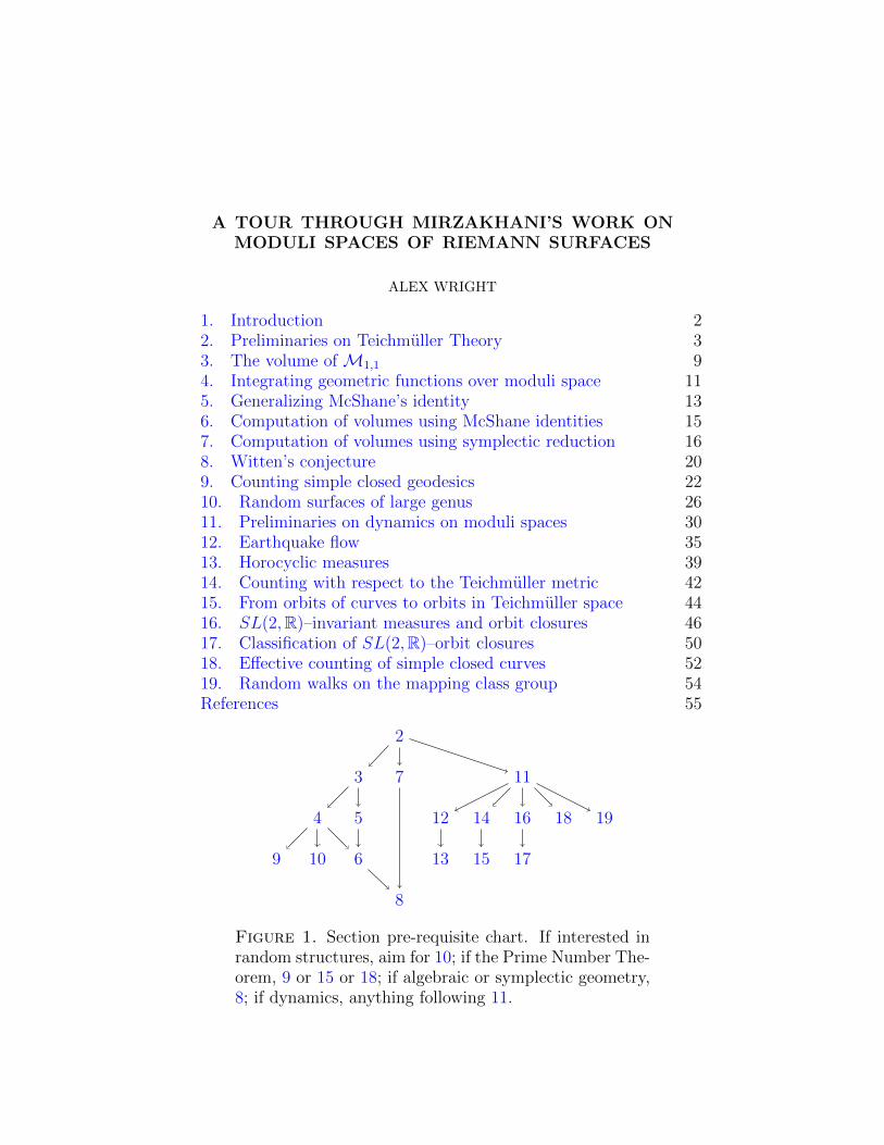
1. Introduction 22. Preliminaries on Teichmuller Theory 33. The volume of M1,1 94. Integrating geometric functions over moduli space 115. Generalizing McShane’s identity 136. Computation of volumes using McShane identities 157. Computation of volumes using symplectic reduction 168. Witten’s conjecture 209. Counting simple closed geodesics 2210. Random surfaces of large genus 2611. Preliminaries on dynamics on moduli spaces 3012. Earthquake flow 3513. Horocyclic measures 3914. Counting with respect to the Teichmuller metric 4215. From orbits of curves to orbits in Teichmuller space 4416. SL(2,R)–invariant measures and orbit closures 4617. Classification of SL(2,R)–orbit closures 5018. Effective counting of simple closed curves 5219. Random walks on the mapping class group 54References 55

2

73 11

54

6

8

9 10

12 14 16

13 15 17

18 19

Figure 1. Section pre-requisite chart. If interested inrandom structures, aim for 10; if the Prime Number The-orem, 9 or 15 or 18; if algebraic or symplectic geometry,8; if dynamics, anything following 11.

2 WRIGHT

1. Introduction

This survey aims to be a tour through Maryam Mirzakhani’s re-markable work on Riemann surfaces, dynamics, and geometry. Thestar characters, all across mathematics and physics as well as in thissurvey, are the moduli spaces Mg,n of Riemann surfaces.

Sections 2 through 10 all relate to Mirzakhani’s study of the sizeof these moduli spaces, as measured by the Weil-Petersson symplecticform. Goldman has shown that many related moduli spaces also havea Weil-Petersson symplectic form, so this can be viewed as part of abroader story [Gol84]. Even more important than the broader story,Mirzakhani’s study unlocks applications to the topology ofMg,n, ran-dom surfaces of large genus, and even geodesics on individual hyper-bolic surfaces.

Sections 11 to 19 reflect the philosophy that Mg,n, despite being atotally inhomogeneous object, enjoys many of the dynamical propertiesof nicer spaces, and even some of the dynamical miracles characteristicof homogeneous spaces. The dynamics of group actions in turn clarifythe geometry of Mg,n and produce otherwise unattainable countingresults.

Our goal is not to provide a comprehensive reference, but ratherto highlight some of the most beautiful and easily understood ideasfrom the roughly 20 papers that constitute Mirzakhani’s work in thisarea. Very roughly speaking, we devote comparable time to each pa-per or closely related group of papers. This means in particular thatwe cannot proportionately discuss the longest paper [EM18], but onthis topic the reader may see the surveys [Zor15,Wri16,Qui16]. Weinclude some open problems, and hope that we have succeeded in con-veying the thriving legacy of Mirzakhani’s research.

We invite the reader to discover for themselves Mirzakhani’s five pa-pers on combinatorics [MM95,Mir96,Mir98,MV15,MV17], wherethe author is not qualified to guide the tour.

We also omit comprehensive citations to work preceding Mirzakhani,suggesting instead that the reader may get off the tour bus at any timeto find more details and context in the references and re-board later,or to revisit the tour locations at a later date. Where possible, wegive references to expository sources, which will be more useful to thelearner than the originals. The reader who consults the references willbe rewarded with views of the vast tapestry of important and beautifulwork that Mirzakhani builds upon, something we can only offer tinyglimpses of here.

MIRZAKHANI’S WORK ON RIEMANN SURFACES 3

We hope that a second year graduate student who has previouslyencountered the definitions of hyperbolic space, Riemann surface, linebundle, symplectic manifold, etc., will be able to read and appreciatethe survey, choosing not to be distracted by the occasional remarkaimed at the experts.

Other surveys on Mirzakhani’s work include [Wol10,Wol13,Do13,McM14,Zor14,Zor15,Hua16,Wri16,Qui16,Mar17,Wri18]. Seealso the issue of the Notices of the AMS that was devoted to Mirzakhani[Not18].

Acknowledgments. We are especially grateful to Scott Wolpert andPeter Zograf for helpfully answering an especially large number of ques-tions, to Paul Apisa for especially detailed comments that resulted inmajor improvements, and to Francisco Arana Herrera, Jayadev Atheya,Alex Eskin, Mike Lipnowski, Curt McMullen, Amir Mohammadi, JuanSouto, Kasra Rafi, and Anton Zorich for in depth conversations.

We also thank the many people who have commented on earlierdrafts, including, in addition to the above, Giovanni Forni, DmitriGekhtman, Mark Greenfield, Chen Lei, Ian Frankel, Athanase Pa-padopoulos, Bram Petri, Feng Zhu, and the anonymous referee.

2. Preliminaries on Teichmuller Theory

We begin with the beautiful and basic results that underlie most ofMirzakhani’s work.

2.1. Hyperbolic geometry and complex analysis. All surfaces areassumed to be orientable and connected. Any simply connected sur-face with a complete Riemannian metric of constant curvature −1 isisometric to the upper half plane

H = {x+ iy | y > 0}endowed with the hyperbolic metric

(ds)2 =(dx)2 + (dy)2

y2.

Perhaps the most important miracle of low dimensional geometry isthat the group of orientation preserving isometries of hyperbolic spaceis equal to the group of biholomorphisms of H. (Both are equal to thegroup PSL(2,R) of Mobius transformations that stabilize the upperhalf plane.)

Every oriented complete hyperbolic surface X has universal coverH, and the deck group acts on H via orientation preserving isometries.Since these isometries are also biholomorphisms, this endows X with

4 WRIGHT

the structure of a Riemann surface, namely an atlas of charts to Cwhose transition functions are biholomorphisms.

Conversely, every Riemann surface X that is not simply connected,not C \ {0}, and not a torus has universal cover H, and the deck groupacts on H via biholomorphisms. Since these biholomorphisms are alsoisometries, this endows X with a complete hyperbolic metric.

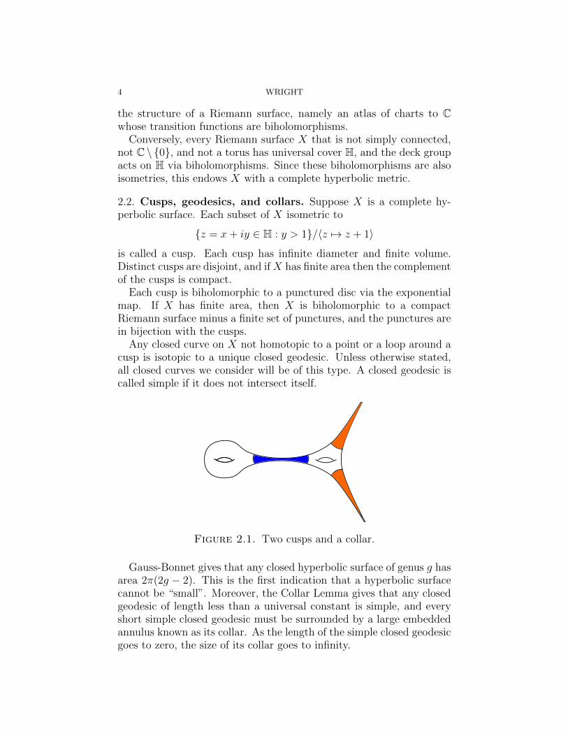
2.2. Cusps, geodesics, and collars. Suppose X is a complete hy-perbolic surface. Each subset of X isometric to

{z = x+ iy ∈ H : y > 1}/〈z 7→ z + 1〉

is called a cusp. Each cusp has infinite diameter and finite volume.Distinct cusps are disjoint, and ifX has finite area then the complementof the cusps is compact.

Each cusp is biholomorphic to a punctured disc via the exponentialmap. If X has finite area, then X is biholomorphic to a compactRiemann surface minus a finite set of punctures, and the punctures arein bijection with the cusps.

Any closed curve on X not homotopic to a point or a loop around acusp is isotopic to a unique closed geodesic. Unless otherwise stated,all closed curves we consider will be of this type. A closed geodesic iscalled simple if it does not intersect itself.

Figure 2.1. Two cusps and a collar.

Gauss-Bonnet gives that any closed hyperbolic surface of genus g hasarea 2π(2g − 2). This is the first indication that a hyperbolic surfacecannot be “small”. Moreover, the Collar Lemma gives that any closedgeodesic of length less than a universal constant is simple, and everyshort simple closed geodesic must be surrounded by a large embeddedannulus known as its collar. As the length of the simple closed geodesicgoes to zero, the size of its collar goes to infinity.

MIRZAKHANI’S WORK ON RIEMANN SURFACES 5

2.3. Building a surface out of pants. A significant amount of thissurvey will concern hyperbolic surfaces with boundary. We will alwaysassume that any surface with boundary that we consider can be isomet-rically embedded in a complete surface so that the boundary consistsof a finite union of closed geodesics.

A hyperbolic sphere with three boundary components is known as apair of pants, or simply as a pants. A fundamental fact gives that, forany three numbers L1, L2, L3 > 0, there is a unique pants with thesethree boundary lengths. Each Li may also be allowed to be zero, inwhich case a pants, now somewhat degenerate, has a cusp instead of aboundary component.

Figure 2.2. Gluing pants to form a genus two surface.

One of the simplest ways to build a closed hyperbolic surface is bygluing together pants. For example, given two pants with the sameboundary lengths, we may glue together the corresponding boundariesto obtain a closed genus 2 surface. In fact, the corresponding bound-aries can be glued using different isometries from the circle to the circle,giving infinitely many genus two hyperbolic surfaces. More complicatedsurfaces can be obtained by gluing together more pants.

2.4. Teichmuller space and moduli space. We define moduli spaceMg,n formally as the set of equivalence classes of oriented genus g hy-perbolic surfaces with n cusps labeled by {1, . . . , n}, where two sur-faces are considered equivalent if they are isometric via an orientationpreserving isometry that respects the labels of the cusps. Equivalently,Mg,n can be defined as the set of equivalence classes of genus g Riemannsurfaces with n punctures labeled by {1, . . . , n}, where two surfaces areconsidered equivalent if they are biholomorphic via a biholomorphismthat respects the labels of the punctures.

We will follow the almost universal abuse of referring to a point inMg,n as a hyperbolic or Riemann surface, leaving out the notationalbookkeeping of the equivalence class.

Teichmuller space Tg,n is defined to be the set

Tg,n = {(X, [φ])}

6 WRIGHT

of points X in Mg,n, which as indicated we think of as hyperbolic orRiemann surfaces, equipped with a homotopy class [φ] of orientationpreserving homeomorphisms φ : Sg,n → X from a fixed oriented topo-logical surface Sg,n of genus g with n punctures. The homotopy class[φ] is called a marking, and one says that Tg,n parametrizes markedhyperbolic or Riemann surfaces.

Let Homeo+(Sg,n) denote the group of orientation preserving home-omorphisms of Sg,n that do not permute the punctures. This group actson Tg,n by precomposition with the marking. The subgroup Homeo+

0 (Sg,n)of homeomorphisms isotopic to the identity acts trivially, so the quo-tient

MCGg,n = Homeo+(Sg,n)/Homeo+0 (Sg,n)

acts on Tg,n. This countable group is called the mapping class group,and

Mg,n = Tg,n/MCGg,n .

Given L = (L1, . . . , Ln) ∈ Rn+, we can similarly define Tg,n(L) to be

the Teichmuller space of oriented genus g hyperbolic surfaces with nboundary components of length L1, . . . , Ln, andMg,n(L) to be the cor-responding moduli space. Here Sg,n is replaced with a genus g surfacewith n boundary circles, and we define Homeo+(Sg,n) to be the orien-tation preserving homeomorphisms that do not permute the boundarycomponents.

It is sometimes convenient to allow Li = 0 in the definitions above,in which case the corresponding boundary is replaced by a cusp. Forexample, using this convention Mg,n =Mg,n(0, . . . , 0).

2.5. Classification of simple closed curves. Let α and β be twodifferent simple closed curves on Sg that are non-separating, in thatcutting either curve does not disconnect the surface. In this case theresult of cutting either α or β is homeomorphic to a genus g−1 surfacewith two boundary curves, and hence are homeomorphic to each other.This homeomorphism can be modified to give rise to a homeomorphismof Sg that takes α to β. In particular, we conclude that there is somef ∈ MCGg such that f([α]) = [β], where [α] denotes the homotopyclass of α.

Next suppose that α is a separating simple closed curve. In this case,Sg \ α has two components, one of which is a surface of genus g1 withone boundary component, and the other of which is a surface of genusg2 = g − g1 with one boundary component. If β is another separatingcurve, then there is some f ∈ MCGg such that f([α]) = [β] if and onlyif the set {g1, g2} arising from β is the same as for α.

MIRZAKHANI’S WORK ON RIEMANN SURFACES 7

In summary, there is a single mapping class group orbit of non-separating simple closed curves on Sg, and bg

2c mapping class group

orbits of separating simple closed curves.

2.6. The twist flow. Let α be a simple closed curve on Sg,n thatisn’t a loop around a cusp. We now introduce the twist flow Twα

t onTeichmuller space as follows. It may be conceptually helpful to startby assuming t is small and positive.

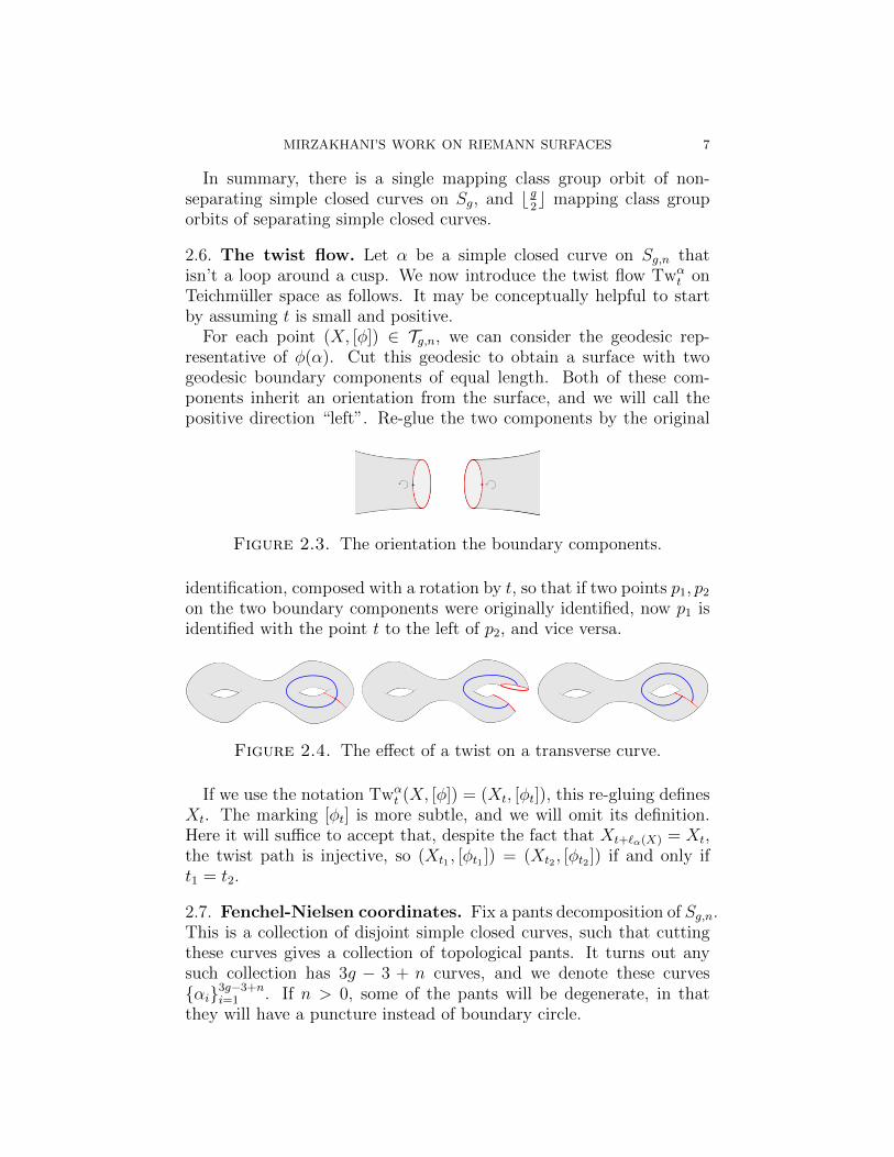
For each point (X, [φ]) ∈ Tg,n, we can consider the geodesic rep-resentative of φ(α). Cut this geodesic to obtain a surface with twogeodesic boundary components of equal length. Both of these com-ponents inherit an orientation from the surface, and we will call thepositive direction “left”. Re-glue the two components by the original

Figure 2.3. The orientation the boundary components.

identification, composed with a rotation by t, so that if two points p1, p2on the two boundary components were originally identified, now p1 isidentified with the point t to the left of p2, and vice versa.

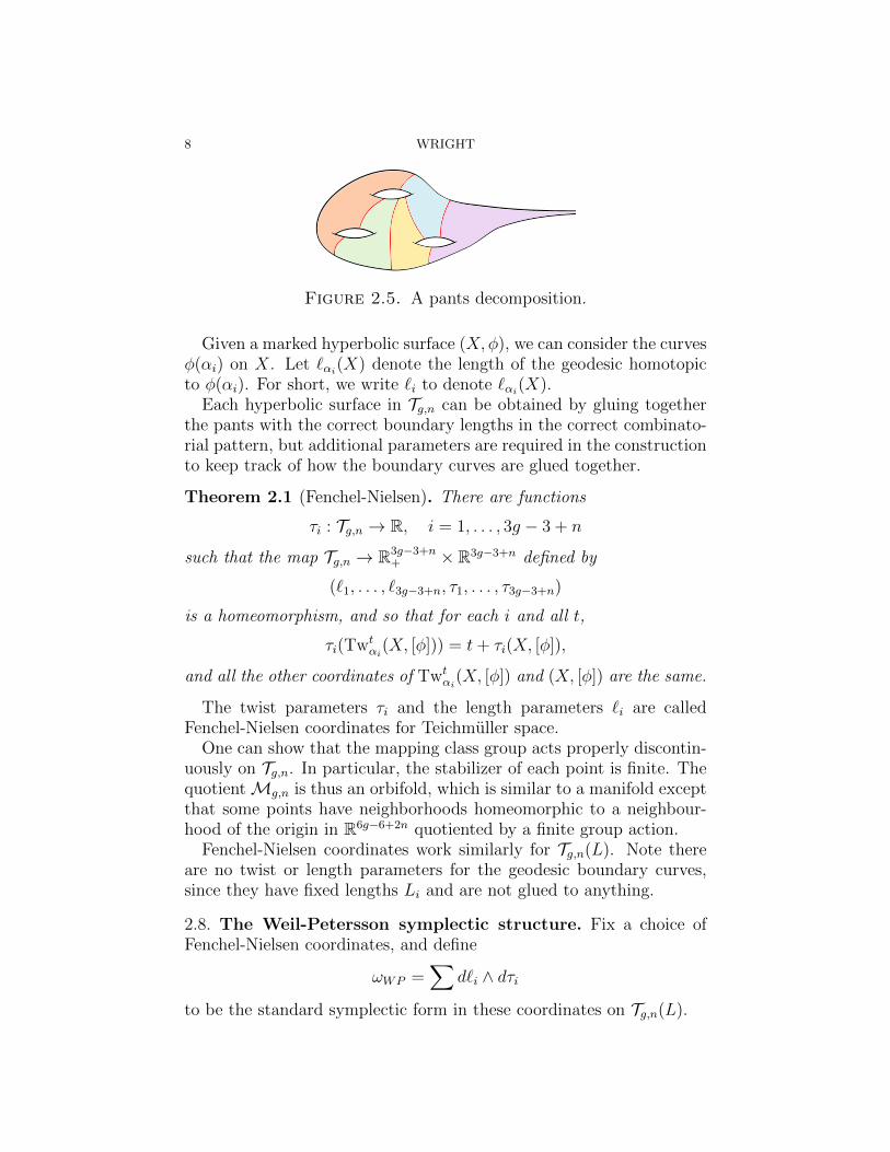
Figure 2.4. The effect of a twist on a transverse curve.

If we use the notation Twαt (X, [φ]) = (Xt, [φt]), this re-gluing defines

Xt. The marking [φt] is more subtle, and we will omit its definition.Here it will suffice to accept that, despite the fact that Xt+`α(X) = Xt,the twist path is injective, so (Xt1 , [φt1 ]) = (Xt2 , [φt2 ]) if and only ift1 = t2.

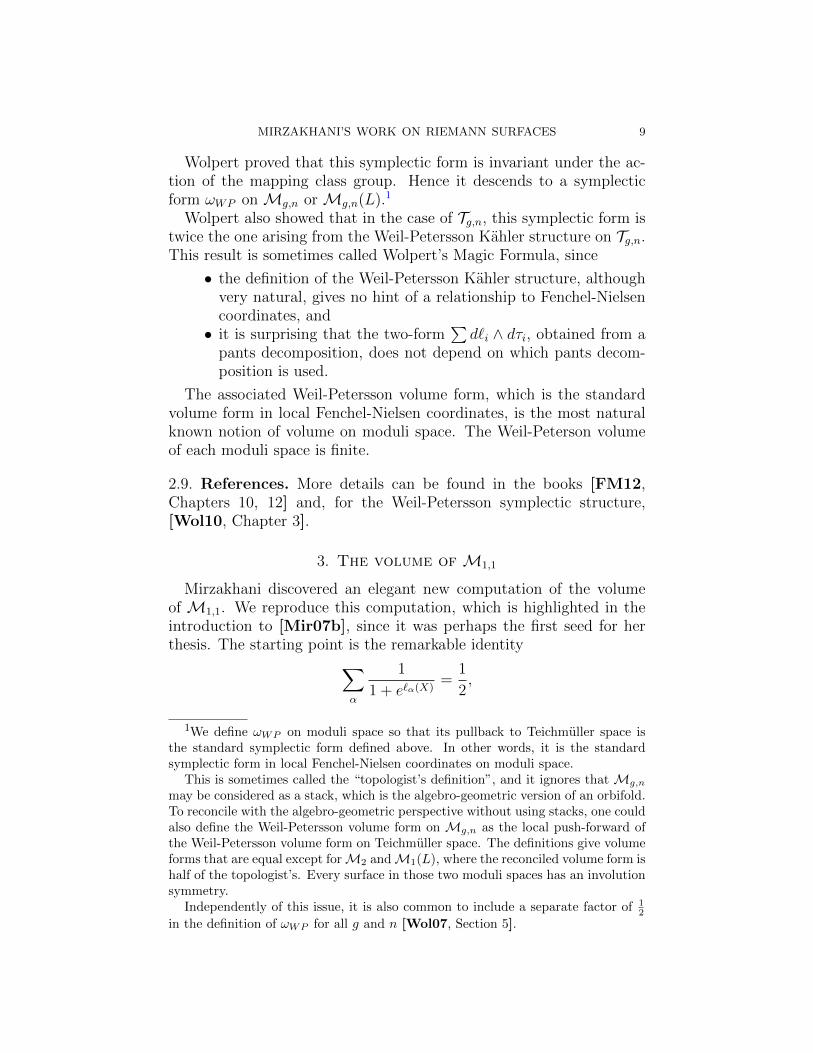
2.7. Fenchel-Nielsen coordinates. Fix a pants decomposition of Sg,n.This is a collection of disjoint simple closed curves, such that cuttingthese curves gives a collection of topological pants. It turns out anysuch collection has 3g − 3 + n curves, and we denote these curves{αi}3g−3+ni=1 . If n > 0, some of the pants will be degenerate, in thatthey will have a puncture instead of boundary circle.

8 WRIGHT

Figure 2.5. A pants decomposition.

Given a marked hyperbolic surface (X,φ), we can consider the curvesφ(αi) on X. Let `αi(X) denote the length of the geodesic homotopicto φ(αi). For short, we write `i to denote `αi(X).

Each hyperbolic surface in Tg,n can be obtained by gluing togetherthe pants with the correct boundary lengths in the correct combinato-rial pattern, but additional parameters are required in the constructionto keep track of how the boundary curves are glued together.

Theorem 2.1 (Fenchel-Nielsen). There are functions

τi : Tg,n → R, i = 1, . . . , 3g − 3 + n

such that the map Tg,n → R3g−3+n+ × R3g−3+n defined by

(`1, . . . , `3g−3+n, τ1, . . . , τ3g−3+n)

is a homeomorphism, and so that for each i and all t,

τi(Twtαi

(X, [φ])) = t+ τi(X, [φ]),

and all the other coordinates of Twtαi

(X, [φ]) and (X, [φ]) are the same.

The twist parameters τi and the length parameters `i are calledFenchel-Nielsen coordinates for Teichmuller space.

One can show that the mapping class group acts properly discontin-uously on Tg,n. In particular, the stabilizer of each point is finite. ThequotientMg,n is thus an orbifold, which is similar to a manifold exceptthat some points have neighborhoods homeomorphic to a neighbour-hood of the origin in R6g−6+2n quotiented by a finite group action.

Fenchel-Nielsen coordinates work similarly for Tg,n(L). Note thereare no twist or length parameters for the geodesic boundary curves,since they have fixed lengths Li and are not glued to anything.

2.8. The Weil-Petersson symplectic structure. Fix a choice ofFenchel-Nielsen coordinates, and define

ωWP =∑

d`i ∧ dτi

to be the standard symplectic form in these coordinates on Tg,n(L).

MIRZAKHANI’S WORK ON RIEMANN SURFACES 9

Wolpert proved that this symplectic form is invariant under the ac-tion of the mapping class group. Hence it descends to a symplecticform ωWP on Mg,n or Mg,n(L).1

Wolpert also showed that in the case of Tg,n, this symplectic form istwice the one arising from the Weil-Petersson Kahler structure on Tg,n.This result is sometimes called Wolpert’s Magic Formula, since

• the definition of the Weil-Petersson Kahler structure, althoughvery natural, gives no hint of a relationship to Fenchel-Nielsencoordinates, and• it is surprising that the two-form

∑d`i ∧ dτi, obtained from a

pants decomposition, does not depend on which pants decom-position is used.

The associated Weil-Petersson volume form, which is the standardvolume form in local Fenchel-Nielsen coordinates, is the most naturalknown notion of volume on moduli space. The Weil-Peterson volumeof each moduli space is finite.

2.9. References. More details can be found in the books [FM12,Chapters 10, 12] and, for the Weil-Petersson symplectic structure,[Wol10, Chapter 3].

3. The volume of M1,1

Mirzakhani discovered an elegant new computation of the volumeof M1,1. We reproduce this computation, which is highlighted in theintroduction to [Mir07b], since it was perhaps the first seed for herthesis. The starting point is the remarkable identity∑

α

1

1 + e`α(X)=

1

2,

1We define ωWP on moduli space so that its pullback to Teichmuller space isthe standard symplectic form defined above. In other words, it is the standardsymplectic form in local Fenchel-Nielsen coordinates on moduli space.

This is sometimes called the “topologist’s definition”, and it ignores that Mg,n

may be considered as a stack, which is the algebro-geometric version of an orbifold.To reconcile with the algebro-geometric perspective without using stacks, one couldalso define the Weil-Petersson volume form on Mg,n as the local push-forward ofthe Weil-Petersson volume form on Teichmuller space. The definitions give volumeforms that are equal except forM2 andM1(L), where the reconciled volume form ishalf of the topologist’s. Every surface in those two moduli spaces has an involutionsymmetry.

Independently of this issue, it is also common to include a separate factor of 12

in the definition of ωWP for all g and n [Wol07, Section 5].

10 WRIGHT

of McShane [McS98], which gives that a certain sum involving thelengths `α(X) of all simple closed geodesics α on X ∈M1,1 is indepen-dent of X ∈M1,1. In Section 5 we’ll explain where this identity comesfrom.

LetM∗1,1 denote the infinite cover ofM1,1 parametrizing pairs (X,α),

where X ∈M1,1 and α is a simple closed geodesic on X. Mirzakhani’scomputation begins

1

2Vol(M1,1) =

∫M1,1

∑α

1

1 + e`X(α)dVolWP

=

∫M∗

1,1

1

1 + e`X(α)dVolWP .

This “unfolding” is justified because the fibers of the mapM∗1,1 →M1

are precisely the set of simple closed geodesics, which is the set beingsummed over in McShane’s identity.

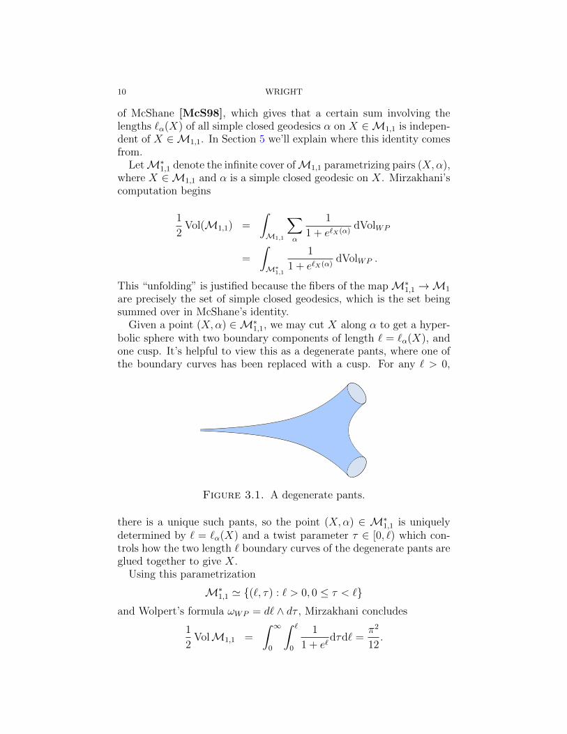
Given a point (X,α) ∈M∗1,1, we may cut X along α to get a hyper-

bolic sphere with two boundary components of length ` = `α(X), andone cusp. It’s helpful to view this as a degenerate pants, where one ofthe boundary curves has been replaced with a cusp. For any ` > 0,

Figure 3.1. A degenerate pants.

there is a unique such pants, so the point (X,α) ∈ M∗1,1 is uniquely

determined by ` = `α(X) and a twist parameter τ ∈ [0, `) which con-trols how the two length ` boundary curves of the degenerate pants areglued together to give X.

Using this parametrization

M∗1,1 ' {(`, τ) : ` > 0, 0 ≤ τ < `}

and Wolpert’s formula ωWP = d` ∧ dτ , Mirzakhani concludes

1

2VolM1,1 =

∫ ∞0

∫ `

0

1

1 + e`dτd` =

π2

12.

MIRZAKHANI’S WORK ON RIEMANN SURFACES 11

4. Integrating geometric functions over moduli space

In this section we give a key result from [Mir07b] that gives a pro-cedure for integrating certain functions over moduli space, generalizingthe “unfolding” step in the previous section.

4.1. A special case. Let γ be a simple non-separating closed curveon a surface of genus g > 2. For a continuous function f : R+ → R+,we define a function fγ :Mg → R by

fγ(X) =∑

[α]∈MCG ·[γ]

f(`α(X)).

Here the sum is over the mapping class group orbit of the homotopyclass [γ] of γ. Soon we will generalize this notation, but for the momentthe subscript may seem strange: since there is only one mapping classgroup orbit of non-separating simple closed curve, for the moment fγdoes not depend on γ.

Recall thatMg−1,2(`, `) is the moduli space of genus g−1 hyperbolicsurfaces with 2 labeled boundary geodesics of length `. We will givean outline of Mirzakhani’s proof that∫

Mg

fγ(X) dVolWP =1

2

∫ ∞0

`f(`) Vol(Mg−1,2(`, `))d`.

Define Mγg to be the set of pairs (X,α), where X ∈ Mg and α is a

geodesic with [α] ∈ MCG ·[γ]. The fibers of the map

Mγg →Mg, (X,α) 7→ X

correspond exactly to the set {[α] ∈ MCG ·[γ]} that is summed over inthe definition of fγ, and in fact∫

Mg

fγ(X) dVolWP =

∫Mγ

g

f(`α(X)) dVolWP .

Cutting X along α almost determines a point ofMg−1,2(`, `), exceptthat the two boundary geodesics are not labeled. However, since thereare two choices of labeling, we can say that there is a two-to-one map

{(`, Y, τ) : ` > 0, Y ∈Mg−1,2(`, `), τ ∈ R/`Z} →Mγg ,

where the map glues together the two boundary components of Y witha twist determined by τ . Wolpert’s Magic Formula determines the

12 WRIGHT

pullback of the Weil-Petersson measure, and we get∫Mγ

g

f(`α(X)) dVolWP =1

2

∫ ∞`=0

∫ `

τ=0

∫Mg−1,2(`,`)

f(`) dVolWP dτd`

=1

2

∫ ∞0

`f(`) Vol(Mg−1,2(`, `))d`.

The case of g = 2 is special, because every Y ∈ M1,2(`, `) has aninvolution exchanging the two boundary components. Because of thisinvolution, one cannot distinguish between the two choices of labelingthe two boundary components, and the map that was two-to-one is nowone-to-one. Thus, the same formula holds in genus 2 with the factor of12

removed.

4.2. The general case. A simple multi-curve, often just multi-curvefor short, is a finite sum of disjoint simple closed curves with positivereal weights, none of whose components are loops around a cusp. Ifγ =

∑ki=1 ciγi is a multi-curve, its length is defined by

`γ(X) =k∑i=1

ci`γi(X).

We define fγ for multi-curves in the same way as above, and note thatfγ in fact only depends on the mapping class group orbit of [γ].

Suppose that cutting the geodesic representative of γ decomposesX ∈Mg,n(L) into s connected components X1, . . . , Xs, and that

• Xj has genus gj,• Xj has nj boundary components, and• the lengths of the boundary components of Xj are given by

Λj ∈ Rnj+ .

If we set `i = `γi(X), then all the entries of each Λj are from {L1, . . . , Ln}(if they correspond to the original boundary of X) or {`1, . . . , `k} (ifthey correspond to the new boundary created by cutting γ).

Theorem 4.1 (Mirzakhani’s Integration Formula). For any multi-

curve γ =∑k

i=1 ciγi,∫Mg,n(L)

fγ dVolWP

= ιγ

∫`=(`1,...,`k)∈Rk+

`1 · · · `kf(c1`1 + · · ·+ ck`k)s∏j=1

Vol(Mgj ,nj(Λj))d`,

MIRZAKHANI’S WORK ON RIEMANN SURFACES 13

where ιγ ∈ Q+ is an explicit constant.2

5. Generalizing McShane’s identity

The starting point for Mirzakhani’s volume computations is the fol-lowing result proven in [Mir07b]. It relies on two explicit functionsD,R : R3

+ → R+ whose exact definitions are omitted here.

Theorem 5.1. For any hyperbolic surface X with n geodesic boundarycircles β1, . . . , βn of lengths L1, . . . , Ln,∑

γ1,γ2

D(L1, `X(γ1), `X(γ2)) +n∑i=2

∑γ

R(L1, Li, `X(γ)) = L1,

where the first sum is over all pairs of closed geodesics γ1, γ2 boundinga pants with β1, and the second sum is over all simple closed geodesicsγ bounding a pants with β1 and βi.

By studying the asymptotics of this formula when some Li → 0, it ispossible to derive a related formula in the case when the boundary βi isreplaced with a cusp. In the case when all βi are replaced with cusps,Mirzakhani recovers identities due to McShane [McS98], including theidentity given in Section 3. Thus, Mirzakhani refers to Theorem 5.1 asthe generalized McShane identities.

2 Slightly different values of the constant have been recorded in different placesin the literature. We believe the correct constant is

ιγ =1

2M [Stab(γ) : 〈S,∩ki=1 Stab+(γi)〉],

where M is the number of i such that γi bounds a torus with no other boundarycomponents and not containing any other component of γ, Stab(γ) is the stabilizerof the weighted multi-curve γ, Stab+(γi) is the subgroup of the mapping class groupthat fixes γi and its orientation, and S is the kernel of the action of the mappingclass group on Teichmuller space. (Note that S is trivial except in the case when(g, n) is (1, 1) or (2, 0), in which case it has size two and is central.) Given twosubgroups H1, H2, we write 〈H1, H2〉 for the subgroup they generate.

The number ι−1γ arises as the degree of a measurable map from

P ={

(`, Y, τ) : ` ∈ Rk+, Y ∈s∏j=1

Mgj ,nj (Λj), τ ∈k∏i=1

R/`iZ}

to the space Mγg,n(L) of pairs (X,α), where X ∈ Mg,n(L) and α is a multi-

geodesic with [α] ∈ MCG ·[γ]. This natural map factors through the spaceMγ,+g,n (L)

of (ordered) tuples (X,α1, . . . , αk), where X ∈ Mg,n(L), and the αi are disjointoriented geodesics with [

∑ciαi] ∈ MCG ·[γ]. The degree of P → Mγ,+

g,n (L) is 2M

and the degree of Mγ,+g,n (L)→Mγ

g,n(L) is the remaining index factor.

14 WRIGHT

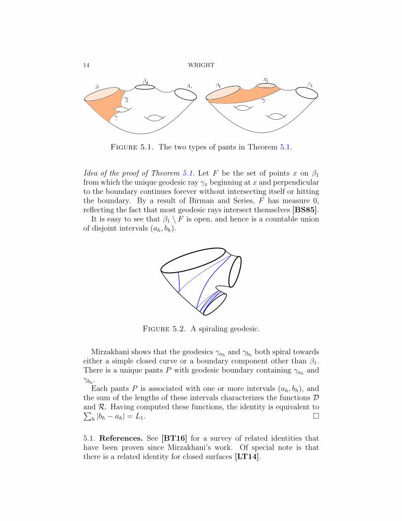
Figure 5.1. The two types of pants in Theorem 5.1.

Idea of the proof of Theorem 5.1. Let F be the set of points x on β1from which the unique geodesic ray γx beginning at x and perpendicularto the boundary continues forever without intersecting itself or hittingthe boundary. By a result of Birman and Series, F has measure 0,reflecting the fact that most geodesic rays intersect themselves [BS85].

It is easy to see that β1 \ F is open, and hence is a countable unionof disjoint intervals (ah, bh).

Figure 5.2. A spiraling geodesic.

Mirzakhani shows that the geodesics γah and γbh both spiral towardseither a simple closed curve or a boundary component other than β1.There is a unique pants P with geodesic boundary containing γah andγbh .

Each pants P is associated with one or more intervals (ah, bh), andthe sum of the lengths of these intervals characterizes the functions Dand R. Having computed these functions, the identity is equivalent to∑

h |bh − ah| = L1. �

5.1. References. See [BT16] for a survey of related identities thathave been proven since Mirzakhani’s work. Of special note is thatthere is a related identity for closed surfaces [LT14].

MIRZAKHANI’S WORK ON RIEMANN SURFACES 15

6. Computation of volumes using McShane identities

We now outline how Mirzakhani used her integration formula andthe generalized McShane identities to recursively compute the Weil-Petersson volumes of Mg,n(L) [Mir07b]. Except in the case of L =(0, . . . , 0), M0,4(L) and M1(L), these volumes were unknown beforeMirzakhani’s work.

As in Section 3, we begin by integrating the generalized McShaneidentity to obtain

L1 Vol(Mg,n(L)) =

∫Mg,n(L)

∑γ1,γ2

D(L1, `X(γ1), `X(γ2)) dVolWP

+

∫Mg,n(L)

n∑i=2

∑γ

R(L1, Li, `X(γ)) dVolWP .

In fact, ∂∂xD(x, y, z) and ∂

∂xR(x, y, z) are nicer functions than D and

R, so Mirzakhani considers the ∂∂L1

derivative of this identity.Let us consider just the sum∑

γ

∂

∂L1

R(L1, L2, `X(γ))

over all simple closed geodesics γ which bound a pants with β1 and β2.The set of such γ is one mapping class group orbit, so we may applyMirzakhani’s Integration Formula to get∫

Mg,n(L)

∑γ

∂

∂L1

R(L1, Li, `X(γ)) dVolWP

= ιγ

∫R+

`∂

∂L1

R(L1, Li, `) Vol(Mg,n−1(`, L2, . . . , Ln))d`.

Note that the surfaces in Mg,n−1(`, L2, . . . , Ln) are smaller thanthose inMg,n(L) in that they have one less pants in a pants decompo-sition.

The sum over pairs γ1, γ2 is similar, but more complicated becausethe set of multi-curves γ1+γ2 that arise consists of a finite but possiblylarge number of mapping class group orbits.

This produces an expression for ∂∂L1

L1 Vol(Mg,n(L)) as a finite sumof integrals involving volumes of smaller moduli spaces. Mirzakhani wasable to compute these integrals, allowing her to compute Vol(Mg,n(L))recursively. These computations imply in particular that Vol(Mg,n(L))

16 WRIGHT

is a polynomial in the L2i whose coefficients are positive rational mul-

tiples of powers of π, which we will reprove from a different point ofview in the next section.

6.1. References. Mirzakhani’s recursions are concisely presented interms of the coefficients of the polynomials in [Mir13, Section 3.1]and [MZ15, Section 2]3. Using these recursions to compute the volumepolynomials is rather slow, because of the combinatorial explosion inhigh genus of the number of different moduli spaces that arise fromrecursively cutting along geodesics. Zograf has given a faster algorithm[Zog08].

Mirzakhani’s results don’t directly allow for the computation of Vol(Mg).However these volumes were previously known via intersection theory.They can also be recovered via the remarkable formula

2πi(2g − 2) Vol(Mg) =∂ Vol(∂Mg,1)

∂L(2πi)

proven in [DN09].It would be interesting to recompute Vol(Mg) using Mirzakhani’s

strategy and the identity for closed surfaces in [BT16].Mirzakhani’s recursions fit into the framework of “topological recur-

sions” [Eyn14].

7. Computation of volumes using symplectic reduction

We now give Mirzakhani’s second point of view on Weil-Peterssonvolumes, from [Mir07c].

7.1. A larger moduli space. Consider the moduli space Mg,n ofgenus g Riemann surfaces with n geodesic boundary circles with amarked point on each boundary circle. This moduli space has dimen-sion 2n greater than that ofMg,n(L), because the length of each bound-ary circle can vary, and the marked point on each boundary circle canvary.

Mg,n admits a version of local Fenchel-Nielsen coordinates, wherein addition to the usual Fenchel-Nielsen coordinates there is a lengthparameter `i for each boundary circle and a parameter that keeps trackof the position the each marked point on each boundary circle. Theparameters keeping track of the marked points are thought of as twist

parameters. The space Mg,n also has a Weil-Peterson form ωWP , which

3Due to a different convention, in these papers the volumes ofM2 andM1,1(L)are half what our conventions give. In the second line of [Mir13, Section 3.1], thereis a typo that should be corrected as d0 = 3g − 3 + n − |d|. In [MZ15, Equation2.13], there is a typo that should be corrected as |I t J | = {2, . . . , n}.

MIRZAKHANI’S WORK ON RIEMANN SURFACES 17

is still described by Wolpert’s Magic Formula, meaning that it is thestandard symplectic form in any system of local Fenchel-Nielsen coor-dinates.

Consider now the function µ : Mg,n → Rn+ defined by

µ =

(`212, . . . ,

`2n2

).

The reason for this definition will become clear in the next subsection.Let S1 = R/Z, and consider the (S1)n action that moves the marked

points along the boundary circles. Each level set µ−1(L21/2, . . . , L

2n/2)

is invariant under the (S1)n action, and the quotient is the spaceMg,n(L1, . . . , Ln) with fixed boundary lengths and no marked pointson the boundary. That is,

Mg,n(L1, . . . , Ln) = µ−1(L21/2, . . . , L

2n/2)/(S1)n.

7.2. Symplectic reduction. We now review a version of the Duistermaat-

Heckman Theorem in symplectic geometry, as it applies to Mg,n.

The symplectic form ωWP on Mg,n provides a non-degenerate bi-

linear form on each tangent space to Mg,n. This gives an identificationbetween the tangent space and its dual, and hence between vector fieldsand one-forms.

Any function H on Mg,n determines a one-form dH and hence alsoa vector field VH defined via this duality. This duality is recordedsymbolically as

dH = ωWP (VH , ·).The flow in the vector field VH is called the Hamiltonian flow of H,and H is called the Hamiltonian function.

To begin, take n = 1. Let `1 : Mg,1 → R+ denote the length of theunique boundary circle, and let τ1 denote the twist coordinate giving

the position of the marked point. The S1 action on Mg,n discussedabove is simply given by τ1 7→ τ1 + t`1, where t ∈ R/Z, and hence isgenerated by the vector field `1∂τ1 . Wolpert’s Magic Formula gives

ωWP (`1∂τ1 , ·) = `1d`1.

If H = `21/2 then dH = `1d`1, so the S1 action is Hamiltonian withHamiltonian function H.

Now take n > 1. Then the i-th coordinate S1 action on Mg,n,which moves the position of the marked point on the i-th boundarycircle, is Hamiltonian with Hamiltonian function `2i /2. Using a naturalway to combine different Hamiltonian functions into a single function

18 WRIGHT

called the moment map, one says that the (S1)n action on Mg,n isHamiltonian with moment map µ given above.

For every ξ = (L21/2, . . . , L

2n/2), the space µ−1(ξ) is the manifold

parameterizing surfaces in Mg,n(L1, . . . , Ln) with a marked point oneach boundary circle, and as we’ve discussed

µ−1(ξ)/(S1)n =Mg,n(L1, . . . , Ln).

The fact that this quotient is a symplectic manifold is an instance of ageneral phenomenon called symplectic reduction.

Return to the case n = 1. Then µ−1(ξ) is a principal circle bundleover Mg,1(L1). (A principal S1 bundle is a bundle with an action ofS1 that is simply transitive on fibers.) Let’s call this circle bundle C1.

Generalizing this to n > 1, we see that µ−1(ξ) → Mg,1(L1, . . . , Ln)is a product of n circle bundles Ci, i = 1, . . . , n. Here Ci can be definedas the spaces of of surfaces in Mg,n(L1, . . . , Ln) together with just asingle marked point on the i-th boundary circle (and no marked pointson any of the other boundary circles).

Theorem 7.1 (Duistermaat-Heckman Theorem). For any fixed ξ andfor t = (t1, . . . , tn) ∈ Rn small enough, there exists a diffeomorphism

φt : µ−1(ξ)/(S1)n → µ−1(ξ + t)/(S1)n

such that

φ∗t (ωWP ) = ωWP +n∑i=1

tic1(Ci),

where c1(Ci) is the first Chern class of the circle bundle Ci over µ−1(ξ+t)/(S1)n. Here, on the left hand side ωWP refers to the Weil-Peterssonform on µ−1(ξ + t)/(S1)n, and on the right hand side it refers to theWeil-Petersson form on µ−1(ξ)/(S1)n.

The reader unfamiliar with Chern classes may in fact take this the-orem to be the definition for this survey; we will not use any otherproperties of Chern classes.

Part of Theorem 7.1 is powered by a relative of the Darboux Theo-rem. The Darboux Theorem states that a neighborhood of any pointin a symplectic manifold is symplectomorphic to the simplest thing youcould guess it to be, namely a neighbourhood in a vector space withthe standard symplectic form.

Here, a neighborhood of µ−1(ξ) is topologically µ−1(ξ)×(−δ, δ)n, andone can create a guess for what the symplectic form ωWP might looklike on µ−1(ξ) × (−δ, δ)n, using ωWP on µ−1(ξ)/(S1)n and curvatureforms for the circle bundles. The Equivariant Coisotropic ReductionTheorem, which is the relative of the Darboux Theorem we referred to,

MIRZAKHANI’S WORK ON RIEMANN SURFACES 19

says that this guess is in fact symplectomorphic to a neighborhood of

µ−1(ξ) in Mg,n.

7.3. Computations of volumes. From Theorem 7.1, Vol(Mg,n(L1, . . . , Ln))is a polynomial in a small neighborhood of any (L1, . . . , Ln), and henceis globally a polynomial. By considering ξ = (ε2/2, . . . , ε2/2), we get

Vol(Mg,n(L1, . . . , Ln))

=1

(3g − 3 + n)!

∫Mg,n(L1,...,Ln)

ω3g−3+nWP

=1

(3g − 3 + n)!

∫Mg,n(ε,...,ε)

(ωWP +

∑ L2i − ε2

2c1(Ci)

)3g−3+n

.

Note that Theorem 7.1 only directly gives this for Li close to ε, butsince the volume is a polynomial it must in fact be true for all Li.Note also that ωWP denotes the Weil-Petersson symplectic form onMg,n(L1, . . . , Ln) in the first integral and onMg,n(ε, . . . , ε) in the sec-ond integral.

Taking a limit as ε→ 0, Mirzakhani obtains

Vol(Mg,n(L1, . . . , Ln)) =1

(3g − 3 + n)!

∫Mg,n

(ωWP +

∑ L2i

2c1(Ci)

)3g−3+n

.

Here Ci can be defined as the circle of points on a horocycle of size 1about the i-th cusp.

One can first interpret this integral in terms of the differential formsrepresenting c1(Ci) produced by the proof of Theorem 7.1. These dif-ferential forms, and the circle bundles Ci, extend continuously to anatural compactification Mg,n constructed by Deligne and Mumford,and so one can and typically does replaceMg,n withMg,n as the spaceto be integrated over. This allows a more topological interpretation ofthe integral as the pairing of a class in H6g−6+2n(Mg) with the funda-mental class of Mg,n.

In summary, we have the following.

Theorem 7.2. The volume of Mg,n(L1, . . . , Ln) is a polynomial∑|α|≤3g−3+n

Cg(α)L2α

whose coefficients Cg(α) are rational multiples of integrals of powers ofthe Chern classes c1(Ci) and the Weil-Petersson symplectic form. Hereα = (α1, . . . , αn), |α| =

∑αi and L2α =

∏L2αii .

We will discuss a number of interesting results and open problemsabout these polynomials in Section 10.

20 WRIGHT

7.4. References. For more on the material relating to symplectic re-duction, see, for example, [CdS01, Chapter 22, 23, 30.2].

The work of Mirzakhani suggests some similarities between modulispaces of Riemann surfaces and spaces of representations of surfacegroups into compact Lie groups modulo conjugacy. These spaces ofrepresentations are also known as character varieties or moduli spacesof stable bundles. Mirzakhani points out the connection between hertechniques and those used previously by Witten and others in thiscontext [Wit92]. See the citations in Mirzakhani’s papers and thesurvey [Jef05] for more details.

8. Witten’s conjecture

We now describe Mirzakhani’s proof of Witten’s conjecture [Mir07c].This brings us to the algebro-geometric perspective on the coefficientsCg(α) from Theorem 7.2.

8.1. Intersection theory. Let Ci and ωWP denote the extensions ofCi and ω from Mg,n to Mg,n.

The class c1(Ci) ∈ H2(Mg,n,Q) is typically denoted ψi, and is muchstudied. One often defines ψi as the first Chern class of a line bundleLi called the relative cotangent bundle at the i-the marked point.

Wolpert showed that the cohomology class [ωWP ] ∈ H2(Mg,n) isequal to 2π2κ1, where κ1 ∈ H2(Mg,n,Q) is the much studied firstkappa class [Wol83]. As a result, all of the coefficients Cg(α) fromTheorem 7.2 are in Q[π2].

The compactificationMg,n is an algebraic variety and a smooth orb-ifold, and the classes ψi and κ1 can be thought of as dual to (equiva-lence classes of) divisors, which are linear combinations of subvarietiesof complex codimension 1. The intersection of two such classes, iftransverse, has complex codimension 2, and similarly the intersectiondimCMg,n = 3g − 3 + n of them, if transverse, is a finite collection ofpoints. Integrals of a product of 3g−3+n of the ψi and κ1 classes, whichup to factors are exactly the coefficients Cg(α), count the number ofpoints of intersection. Thus, they are called intersection numbers. Seethe book [LZ04, Chapter 4.6] for some example computations usingthis point of view.

It is hard for the uninitiated to fathom how much useful informationsuch intersection numbers can contain, so we pause to give just a fewpoints of motivation.

• They are central to the study of the geometry of Mg,n.

MIRZAKHANI’S WORK ON RIEMANN SURFACES 21

• By Theorem 7.1 they determine Weil-Petersson volumes. Laterwe will see that these volumes can be used to understand thegeometry of Weil-Petersson random surfaces.• They appear in theoretical physics [Wit91].• They determine counts of combinatorial objects called ribbon

graphs [Kon92].• They determine Hurwitz numbers, which count certain branched

coverings of the sphere, or equivalently factorizations of permu-tations into transpositions [ELSV01].

8.2. A generating function for intersection numbers. Make thenotational convention

〈τd1 · · · τdn〉g =

∫Mg,n

ψd11 . . . ψdnn .

Unless∑di = 3g − 3 + n, this is defined to be zero. Note that

“〈τd1 · · · τdn〉g” should be considered as a single mathematical symbol,and the order of the di’s doesn’t matter.

Define the generating function for top intersection products in genusg by

Fg(t0, t1, . . .) =∑n

1

n!

∑d1,...,dn

〈∏

τdi〉gtd1 · · · tdn ,

where the sum is over all non-negative sequences (d1, . . . , dn) such that∑di = 3g − 3 + n. One can then form the generating function

F =∑g

λ2g−2Fg,

which arises as a partition function in 2D quantum gravity. Note thatF is a generating function in infinitely many variables: λ keeps trackof the genus, and td keeps track of the number of d-th powers of psiclasses.

Witten’s conjecture is equivalent to the fact that eF is annihilatedby a sequence of differential operators

L−1, L0, L1, L2, . . .

satisfying the Virasoro relations

[Lm, Lk] = (m− k)Lm+k.

22 WRIGHT

To give an idea of the complexity of these operators, we record theformula for Ln, n > 0:

Ln = −(2n+ 3)!!

2n+1

∂

∂tn+1

+1

2n+1

∞∑k=0

(2k + 2n+ 1)!!

(2k − 1)!!tk

∂

∂tn+k

+1

2n+2

∑i+j=n−1

(2i+ 1)!!(2k + 1)!!∂2

∂ti∂tj.

The equations Li(eF ) = 0 encode recursions among the intersection

numbers, which appear as the constant terms in Mirzakhani’s volumepolynomials. These recursions allow for the computation of all intersec-tion numbers of psi classes. Mirzakhani showed that these recursionsfollow from her recursive formulas for the volume polynomials, thusgiving a new proof of Witten’s conjecture.

8.3. A brief history. Witten’s conjecture was published in 1991, mo-tivated by physical intuition that two different models for 2D quantumgravity should be equivalent [Wit91]. Kontsevich published a proof in1992, using a combinatorial model forMg,n arising from Strebel differ-entials, ribbon graphs, and random matrices [Kon92]. This work wascentral in his 1998 Fields Medal citation.

It wasn’t until 2007 that Mirzakhani’s proof was published, andaround the same time other proofs appeared. Later, Do related Mirza-khani’s and Kontsevich’s proofs, recovering Kontsevich’s formula forthe number of ribbon graphs by considering asymptotics of the Weil-Petersson volume polynomials, using that a rescaled Riemann surfacewith very large geodesic boundary looks like a graph [Do10].

9. Counting simple closed geodesics

Let X be a complete hyperbolic surface, and let cX(L) be the num-ber of primitive closed geodesics of length at most L on X. Primitivemeans simply that the geodesic does not traverse the same path mul-tiple times. The famous Prime Number Theorem for Geodesics givesthe asymptotic

cX(L) ∼ 1

2

eL

L

as L→∞. (The factor of 12

disappears if one counts primitive orientedgeodesics, since there are two orientations on each closed geodesic.)

MIRZAKHANI’S WORK ON RIEMANN SURFACES 23

Amazingly, this doesn’t depend on which surface X we choose, or eventhe genus of X.

In [Mir08b], Mirzakhani proved that the number of closed geodesicsof length at most L on X that don’t intersect themselves is asymptoticto a constant depending on X times L6g−6+2n. That this asymptoticis polynomial rather than exponential reflects the extreme unlikelinessthat a random closed geodesic is simple, in the same spirit as the resultof Birman and Series mentioned in Section 5.

In fact Mirzakhani proved a more general result. For any rationalmulti-curve γ, she considered

sX(L, γ) = |{α ∈ MCG ·γ : `α(X) ≤ L}|.In other words, sX(L, γ) counts the number of closed multi-geodesicsα on X of length less than L that are “of the same topological type”as γ.

The set of simple closed curves forms finitely many mapping classgroup orbits. So by summing finitely many of these functions sX(L, γ),one gets the corresponding count for all simple closed curves.

Theorem 9.1. For any rational multi-curve γ,

limL→∞

sX(L, γ)

L6g−6+2n=c(γ) ·B(X)

bg,n,

where c(γ) ∈ Q+, B : Mg,n → R+ is a proper, continuous functionwith a simple geometric definition, and bg,n =

∫Mg,n

B(X) dVolWP .

Eskin-Mirzakhani-Mohammadi have recently given a new proof ofTheorem 9.1 that gives an error term, which we will discuss in Section18, and Erlandsson-Souto have also given a new proof [ES19]. Here weoutline the original proof, after first commenting on one application.

9.1. Relative frequencies. Consider, for example, the case (g, n) =(2, 0) of closed genus 2 surfaces, just to be concrete. The set of simpleclosed curves consists of two mapping class groups orbits: the orbit ofa non-separating curve γns and the orbit of a curve γsep that separatesthe surface into two genus one subsurfaces.

The fact that the limit in Theorem 9.1 is the product of a functionof γ and a function of X has the following consequence: A very longsimple closed curve on X, chosen at random among all such curves,has probability about

c(γsep)

c(γns) + c(γsep)

of being separating. Remarkably, this probability is computable anddoes not depend on X!

24 WRIGHT

Even more remarkably, recent discoveries prove that the same prob-abilities appear in discrete problems about surfaces assembled out offinitely many unit squares [DGZZ,AH19].

9.2. The space of measured foliations. The space of rational multi-curves admits a natural completion called the space MF of measuredfoliations. Later we will delve into measured foliations, but here weonly need a few properties of this space.

• MF is homeomorphic to R6g−6+2n.• MF does not carry a natural linear structure. The most super-

ficial indication of this is that any closed curve α gives a pointofMF , but there is no “−α” inMF , because multi-curves aredefined to have positive coefficients. There is however a naturalaction of R+ on MF , which on multi-curves simply multipliesthe coefficients by t ∈ R+.• MF has a natural piece-wise linear integral structure, that is,

an atlas of charts to R6g−6+2n whose transition functions arepiece-wise in GL(n,Z).• Define the integral points of MF as the set MF(Z) ⊂ MF

of points mapping to Z6g−6+2n under the charts. Define therational pointsMF(Q) similarly. Then integral (resp. rational)points of MF parametrize homotopy classes of integral (resp.rational) multi-curves on the surface.• Any X ∈Mg,n defines a continuous length function

MF → R+, λ→ `λ(X)

whose restriction to multi-curves gives the hyperbolic length ofthe geodesic representative of the multi-curve on X. In partic-ular, `tλ(X) = t`λ(X) for all t ∈ R.

9.3. Warm up. How many points of Z2 ⊂ R2 have length at most L?It is equivalent to ask about the number of points of 1

LZ2 contained in

the unit ball.Recall that the Lebesgue measure can be defined as the limit as

L→∞ of1

L2

∑α∈Z2

δ 1Lα,

where δx denotes the point mass at x. Hence the number of points of1LZ2 contained in the unit ball is asymptotic to L2 times the Lebesgue

measure of the unit ball.

MIRZAKHANI’S WORK ON RIEMANN SURFACES 25

9.4. The Thurston measure. Let’s start with the easy question ofasymptotics for the number

SX(L) = |{α ∈MF(Z) : `α(X) ≤ L}|of all integral multi-curves of length at most L. Using `tλ(X) = t`λ(X),we observe that

SX(L) = |{α ∈ L−1MF(Z) : `α(X) ≤ 1}|.It’s now useful to define the “unit ball”

BX = {α ∈MF : `α(X) ≤ 1}and the measures

µL =1

L6g−6+2n

∑α∈MF(Z)

δ 1Lα.

With these definitions,

SX(L) = L6g−6+2nµL(BX).

As in our warm up, the measures µL converge to a natural Lebesgueclass measure µTh on MF . This measure µTh is called the Thurstonmeasure and is Lebesgue measure in the charts mentioned above. If wedefine B(X) = µTh(BX), we get the asymptotic

SX(L) ∼ B(X)L6g−6+2n.

9.5. The proof. Mirzakhani’s approach to Theorem 9.1 similarly de-fines measures

µLγ =1

L6g−6+2n

∑α∈MCG ·γ

δ 1Lα.

As above, to prove Theorem 9.1, it suffices to show the convergence ofmeasures

µLγ →c(γ)

bg,nµTh.

Using the Banach-Alaoglu Theorem, it isn’t hard to show that thereare subsequences Li →∞ such that µLiγ converges to some measure µ∞γ ,which might a priori depend on which subsequence we pick. To proveTheorem 9.1 it suffices to show that, no matter which such subsequencewe use, we have

µ∞γ =c(γ)

bg,nµTh.

By definition, µLγ ≤ µL, since the mapping class group orbit of γ is

a subset of MF(Z). Since µL converges to the Thurston measure, weget that µ∞γ ≤ µTh.

26 WRIGHT

Since µLγ is mapping class group invariant, the same is true for µ∞γ .A result of Masur in ergodic theory, which we will discuss in Section13, gives that any mapping class group invariant measure onMF thatis absolutely continuous to µTh must be a multiple of µTh [Mas85].

So µLγ ≤ µL = cµTh for some c ≥ 0. At this point in the argumentas far as we know c could depend on the subsequence of Li.

Unraveling the definitions, we have that

(9.5.1)sX(Li, γ)

L6g−6+2ni

→ c ·B(X),

for any X ∈Mg,n. Writing

sX(Li, γ) =∑

α∈MCG γ

χ[0,Li](`α(X)),

we recognize the type of function that Mirzakhani’s Integration For-mula applies to. By integrating the left hand side of (9.5.1) over moduli

space, Mirzakhani is able to prove that c = c(γ)bg,n

as desired. On the one

hand, the integral of cB(X) is c · bg,n. On the other hand, the limit

c(γ) of the integral of sX(Li,γ)

L6g−6+2ni

is easily expressed in terms of the leading

order term in one of Mirzakhani’s volume polynomials.

9.6. Open problems. We will return to counting later, but for nowwe mention the following.

Problem 9.2. Prove an analogue of Theorem 9.1 for non-orientablehyperbolic surfaces.

An example is known already with asymptotics Lδ with δ non-integral[Mag17]. See [Gen17] for a more precise conjecture, as well as a num-ber of related open problems and an analogy between moduli spacesof non-oriented hyperbolic surfaces and infinite volume geometricallyfinite hyperbolic manifolds.

10. Random surfaces of large genus

Given a random d-regular graph with many vertices, what is thechance that it contains a short loop? Is a random graph easy to cut intwo? What properties can be expected of the graph Laplacian?

Mirzakhani considered analogues of these well-studied questions forWeil-Petersson random Riemann surfaces [Mir13,MZ15,MP17], anddevoted her 2010 talk at the International Congress of Mathematiciansto this topic [Mir10].

In this section we discuss this work. We will leave out the backgroundon graphs, but many readers will wish to keep in mind the comparison

MIRZAKHANI’S WORK ON RIEMANN SURFACES 27

between a random d-regular graph, with d fixed and a large number ofvertices, and a random surface with large genus.

10.1. Understanding the volume polynomials. We begin with theconstant term of the polynomial Vol(Mg,n(L)), which is the volumeVg,n ofMg,n. Improving on previous results of Mirzakhani and others,Mirzakhani and Zograf proved the following [Mir13,MZ15].

Theorem 10.1. There exists a universal constant C ∈ (0,∞) suchthat for any fixed n, Vg,n is asymptotic to

C(2g − 3 + n)!(4π2)2g−3+n

√g

as g →∞.

This largely verified a previous conjecture of Zograf, except that hisprediction that C = 1√

πis still open [Zog08]. Mirzakhani and Zograf

also gave a more detailed asymptotic expansion. The proof uses therecursions satisfied by Vg,n discussed in Section 6.

Previous results gave asymptotics as n → ∞ for fixed g [MZ00].See [Mir13, Section 1.4] for open questions concerning asymptotics asboth g and n go to infinity.

Also by studying recursions, Mirzakhani proved results in [Mir13]that imply

(10.1.1) Vol(Mg,n(L)) ≤ Vg,n

n∏i=1

sinh(Li/2)

Li/2.

Mirzakhani and Petri showed this bound is asymptotically sharp forfixed n and bounded L as g →∞ [MP17, Proposition 3.1]. The proofof the inequality actually gives a bound with sinh replaced with one ofits Taylor polynomials.

10.2. An example. To illustrate Mirzakhani’s techniques, we will givean upper bound for the probability that a random surface in Mg hasa non-separating simple closed geodesic of length at most some smallε > 0.

We begin by studying the average overMg of the number of simple,non-separating geodesics of length at most ε on X ∈ Mg. If γ is asimple non-separating curve, we can express this as

1

Vg

∫Mg

∑α∈MCG ·γ

χ[0,ε](`α(X)) dVolWP ,

28 WRIGHT

where χ[0,ε] is the characteristic function of the interval [0, ε]. Mirza-khani’s Integration Formula gives that this is equal to a constant times

1

Vg

∫ ε

0

`Vol(Mg−1,2(`, `))d`.

Since ` is small, inequality (10.1.1) gives that Vol(Mg−1,2(`, `)) is ap-proximately equal to the constant term Vg−1,2 of the volume polyno-mial, so the average is approximately a constant times

Vg−1,2Vg

ε2.

The asymptotics in Theorem 10.1 imply that Vg−1,2

Vgconverges to 1 as

g → ∞, so we get that the average number of simple, non-separatinggeodesics of length at most ε is asymptotic, as g → ∞, to a constanttimes ε2. In particular, this implies that the probability that a randomsurface in Mg has such a geodesic is bounded above by a constanttimes ε2.

A similar lower bound is possible by giving upper bounds for theaverage number of pairs of non-separating simple closed curves.

10.3. Results. Here is an overview of results from [Mir13], whichconcern random X ∈Mg as g →∞.

• The probability that X has a geodesic of length at most ε isbounded above and below by a constant times ε2.• The probability that X has a separating geodesic of length at

most 1.99 log(g) goes to 0.• The probability that X has Cheeger constant less than 0.099

goes to 0.• The probability that λ1(X), the first eigenvalue of the Lapla-

cian, is less than 0.002 goes to 0.• The probability that the diameter of X is greater than 40 log(g)

goes to 0.• The probability that X has an embedded ball of radius at least

log(g)/6 goes to 1.

The first two results are proven using the techniques in the example.The Cheeger constant is defined as

h(X) = infα

`(α)

min(Area(X1),Area(X2)),

where the infimum is over all smooth multi-curves α that cutX into twosubsurfaces X1, X2. Mirzakhani defines the geodesic Cheeger constant

MIRZAKHANI’S WORK ON RIEMANN SURFACES 29

H(X) to be the same quantity where α is required to be a geodesicmulti-curve, so obviously h(X) ≤ H(X). She proves that

H(X)

H(X) + 1≤ h(X),

and is then able to study H(X) using the techniques in the example.The result on λ1 follows from the Cheeger inequality λ1 ≥ h(X)2/4.

We conclude with a special case of the main result of Mirzakhaniand Petri [MP17].

Theorem 10.2. For any 0 < a < b, the number of primitive closedgeodesics of length in [a, b], viewed as a random variable on Mg, con-verges to a Poisson distribution as g →∞.

What is fascinating about this result of Mirzakhani and Petri is thatit concerns all primitive closed geodesics, not just the simple ones. Theproof uses that a geodesic γ of length at most a constant b on a surfaceX of very large genus is contained in a subsurface of bounded genusand with a bounded number of boundary components (depending on b).The boundary of that subsurface is a simple multi-curve β associatedto γ. By showing that, as g → ∞, most X do not have a separatingmulti-curve of bounded length, they are able to show that on mostX most primitive geodesics are simple, and hence use the techniquesillustrated in the example.

10.4. Open problems. For some problems, we list an easier versionfollowed by a harder version.

Problem 10.3. Does there exist a sequence of Riemann surfaces Xn

of genus going to infinity with λ1(Xn)→ 14? Does λ1 converge to 1

4in

probability as g →∞?

Problem 10.4. Is it true that for all g there is an X ∈Mg such thatλ1(X) > 1/4? Is lim infg→∞ Prob(λ1 >

14) > 0?

Problem 10.5. Is there an ε > 0 so that Prob(h ≤ 1 − ε) → 1 asg →∞? Is there an ε > 0 so that there are no surfaces with h > 1− εin sufficiently high genus?

Following conversations with Mike Lipnowski, the author finds itplausible that all three problems have a positive answer. A version ofthe first part of the first problem appears as [WX18, Conjecture 5].

Mirzakhani was also interested discrete models of random surfaces,resulting from gluing together triangles [BM04], and in the collectionof all covers of a fixed surface.

30 WRIGHT

Problem 10.6. Fix X ∈ M2 and ε > 0. Is there a C > 0 such thatfor every g > 2, every Y ∈ Mg with no geodesic of length less thanε has Teichmuller distance at most C from some (unramified) cover ofX?

11. Preliminaries on dynamics on moduli spaces

This section will introduce the central concepts for the remainder ofour tour.

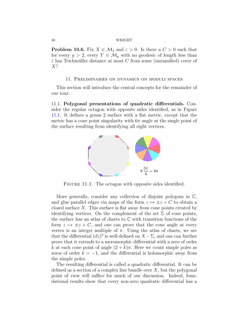
11.1. Polygonal presentations of quadratic differentials. Con-sider the regular octagon with opposite sides identified, as in Figure11.1. It defines a genus 2 surface with a flat metric, except that themetric has a cone point singularity with 6π angle at the single point ofthe surface resulting from identifying all eight vertices.

Figure 11.1. The octagon with opposite sides identified.

More generally, consider any collection of disjoint polygons in C,and glue parallel edges via maps of the form z 7→ ±z + C to obtain aclosed surface X. This surface is flat away from cone points created byidentifying vertices. On the complement of the set Σ of cone points,the surface has an atlas of charts to C with transition functions of theform z 7→ ±z + C, and one can prove that the cone angle at everyvertex is an integer multiple of π. Using the atlas of charts, we seethat the differential (dz)2 is well-defined on X−Σ, and one can furtherprove that it extends to a meromorphic differential with a zero of orderk at each cone point of angle (2 + k)π. Here we count simple poles aszeros of order k = −1, and the differential is holomorphic away fromthe simple poles.

The resulting differential is called a quadratic differential. It can bedefined as a section of a complex line bundle over X, but the polygonalpoint of view will suffice for much of our discussion. Indeed, foun-dational results show that every non-zero quadratic differential has a

MIRZAKHANI’S WORK ON RIEMANN SURFACES 31

polygonal presentation as above, and two polygonal presentations de-fine the same quadratic differential if and only if they are related by asequence of cut and paste moves. Typically it will be implicit that thequadratic differentials we discuss are non-zero.

The simplest quadratic differential is (dz)2 defined on the complexplane. Since it is invariant under translations, it descends to give a qua-dratic differential, which we will also call (dz)2, on the torus C/Z[i]. Apolygonal presentation is the 1 by 1 square with opposite sides identi-fied.

See, for example, [Wri15b, Section 1] for more details on the mate-rial in this subsection and the next.

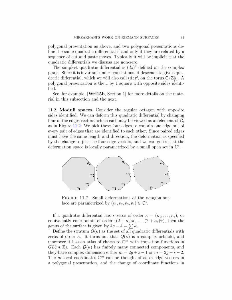
11.2. Moduli spaces. Consider the regular octagon with oppositesides identified. We can deform this quadratic differential by changingfour of the edges vectors, which each may be viewed as an element of C,as in Figure 11.2. We pick these four edges to contain one edge out ofevery pair of edges that are identified to each other. Since paired edgesmust have the same length and direction, the deformation is specifiedby the change to just the four edge vectors, and we can guess that thedeformation space is locally parametrized by a small open set in C4.

Figure 11.2. Small deformations of the octagon sur-face are parametrized by (v1, v2, v3, v4) ∈ C4.

If a quadratic differential has s zeros of order κ = (κ1, . . . , κs), orequivalently cone points of order ((2 + κ1)π, . . . , (2 + κs)π), then thegenus of the surface is given by 4g − 4 =

∑κi.

Define the stratum Q(κ) as the set of all quadratic differentials withzeros of order κ. It turns out that Q(κ) is a complex orbifold, andmoreover it has an atlas of charts to Cm with transition functions inGL(m,Z). Each Q(κ) has finitely many connected components, andthey have complex dimension either m = 2g+ s− 1 or m = 2g+ s− 2.The m local coordinates Cm can be thought of as m edge vectors ina polygonal presentation, and the change of coordinate functions in

32 WRIGHT

GL(m,Z) correspond to doing a cut and paste and picking new edgesvectors.

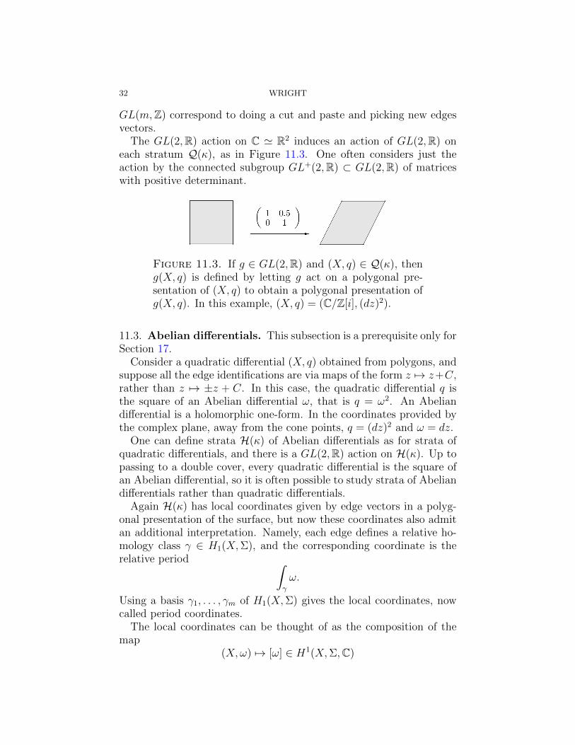
The GL(2,R) action on C ' R2 induces an action of GL(2,R) oneach stratum Q(κ), as in Figure 11.3. One often considers just theaction by the connected subgroup GL+(2,R) ⊂ GL(2,R) of matriceswith positive determinant.

Figure 11.3. If g ∈ GL(2,R) and (X, q) ∈ Q(κ), theng(X, q) is defined by letting g act on a polygonal pre-sentation of (X, q) to obtain a polygonal presentation ofg(X, q). In this example, (X, q) = (C/Z[i], (dz)2).

11.3. Abelian differentials. This subsection is a prerequisite only forSection 17.

Consider a quadratic differential (X, q) obtained from polygons, andsuppose all the edge identifications are via maps of the form z 7→ z+C,rather than z 7→ ±z + C. In this case, the quadratic differential q isthe square of an Abelian differential ω, that is q = ω2. An Abeliandifferential is a holomorphic one-form. In the coordinates provided bythe complex plane, away from the cone points, q = (dz)2 and ω = dz.

One can define strata H(κ) of Abelian differentials as for strata ofquadratic differentials, and there is a GL(2,R) action on H(κ). Up topassing to a double cover, every quadratic differential is the square ofan Abelian differential, so it is often possible to study strata of Abeliandifferentials rather than quadratic differentials.

Again H(κ) has local coordinates given by edge vectors in a polyg-onal presentation of the surface, but now these coordinates also admitan additional interpretation. Namely, each edge defines a relative ho-mology class γ ∈ H1(X,Σ), and the corresponding coordinate is therelative period ∫

γ

ω.

Using a basis γ1, . . . , γm of H1(X,Σ) gives the local coordinates, nowcalled period coordinates.

The local coordinates can be thought of as the composition of themap

(X,ω) 7→ [ω] ∈ H1(X,Σ,C)

MIRZAKHANI’S WORK ON RIEMANN SURFACES 33

with an isomorphism H1(X,Σ,C) ' Cm. Here [ω] denotes the relativecohomology class of ω.

11.4. Relationship to Teichmuller Theory. Orbits of

gt =

(et 00 e−t

)⊂ GL+(2,R)

project via (X, q) → X to geodesics in Mg for a natural metric onMg,n called the Teichmuller metric. Orbits of GL+(2,R) project toholomorphic and isometric immersions of the hyperbolic plane H intoMg called Teichmuller discs or complex geodesics.

The Teichmuller distance d(X, Y ) between two Riemann surfacesX, Y ∈ Mg,n measures how non-conformal a map X → Y must be.The Teichmuller metric is complete, and each pair of points in Tg,n arejoined by a unique Teichmuller geodesic.

11.5. Measured foliations and laminations. This subsection is aprerequisite only for Sections 12 and 13.

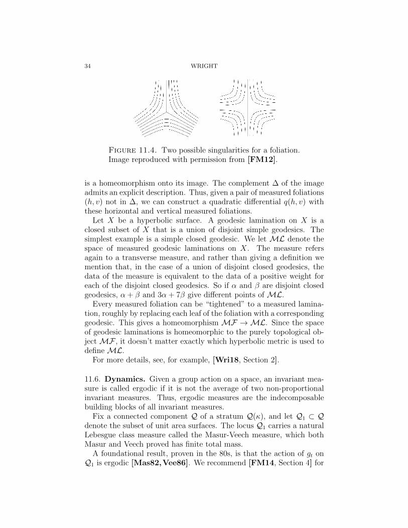
Every quadratic differential (X, q) defines a flat metric with conesingularities on the surface, but in fact it defines a bit more structurethan that. Note that the atlas of charts away from the singularities havetransition functions of the form z 7→ ±z + C, and a general isometryof R2 does not have this form. For example, rotations are not allowedas transition functions.

Because z 7→ ±z +C preserves the vertical and horizontal foliationsof C, we find that each quadratic differential defines vertical and hor-izontal foliations called h(q) and v(q) on the surface. These foliationsare singular at the zeros (cone points) of the quadratic differential, asin Figure 11.4. They also come equipped with some extra structurecalled a transverse measure, which assigns to each arc on the surface anon-negative real number measuring the extent to which the arc crossesthe foliation. (So an arc contained in a leaf of the foliation has 0 trans-verse measure, and the measure of any arc does not change when thearc is pushed along leaves of the foliation.) A foliation equipped witha transverse measure is called a measured foliation.

Let MF be the space of measured foliations on a surface of fixedgenus, up to a natural notion of equivalence. LetQTg,n be the bundle ofnon-zero quadratic differentials over Teichmuller space, and let QMg,n

be the corresponding bundle over moduli space. A foundational resultgives that the map

QTg,n →MF ×MF , (X, q) 7→ (h(q), v(q))

34 WRIGHT

Figure 11.4. Two possible singularities for a foliation.Image reproduced with permission from [FM12].

is a homeomorphism onto its image. The complement ∆ of the imageadmits an explicit description. Thus, given a pair of measured foliations(h, v) not in ∆, we can construct a quadratic differential q(h, v) withthese horizontal and vertical measured foliations.

Let X be a hyperbolic surface. A geodesic lamination on X is aclosed subset of X that is a union of disjoint simple geodesics. Thesimplest example is a simple closed geodesic. We let ML denote thespace of measured geodesic laminations on X. The measure refersagain to a transverse measure, and rather than giving a definition wemention that, in the case of a union of disjoint closed geodesics, thedata of the measure is equivalent to the data of a positive weight foreach of the disjoint closed geodesics. So if α and β are disjoint closedgeodesics, α + β and 3α + 7β give different points of ML.

Every measured foliation can be “tightened” to a measured lamina-tion, roughly by replacing each leaf of the foliation with a correspondinggeodesic. This gives a homeomorphism MF →ML. Since the spaceof geodesic laminations is homeomorphic to the purely topological ob-jectMF , it doesn’t matter exactly which hyperbolic metric is used todefine ML.

For more details, see, for example, [Wri18, Section 2].

11.6. Dynamics. Given a group action on a space, an invariant mea-sure is called ergodic if it is not the average of two non-proportionalinvariant measures. Thus, ergodic measures are the indecomposablebuilding blocks of all invariant measures.

Fix a connected component Q of a stratum Q(κ), and let Q1 ⊂ Qdenote the subset of unit area surfaces. The locus Q1 carries a naturalLebesgue class measure called the Masur-Veech measure, which bothMasur and Veech proved has finite total mass.

A foundational result, proven in the 80s, is that the action of gt onQ1 is ergodic [Mas82,Vee86]. We recommend [FM14, Section 4] for

MIRZAKHANI’S WORK ON RIEMANN SURFACES 35

an expository account of a proof using modern tools. Ergodicity hereis equivalent to the fact that almost every gt-orbit is equidistributed.

A corollary, which was originally due to Masur [Mas85] and alsofollows very easily from the Mautner Lemma (see, for example, [BM00,Lemma 3.6]), is that the action of

ut =

(1 t0 1

)on Q1 is also ergodic.

Another corollary, which follows from a general result called theHowe-Moore Theorem (see, for example, [BM00]), is that the actionof gt is not just ergodic but mixing. This means that, not only do orbitsegments {gt(X, q) : 0 ≤ t ≤ T} equidistribute as T → ∞, but if oneconsiders a nice positive measure set S, then the sets gT (S) equidis-tribute as T →∞.

11.7. Hyperbolicity. Consider a quadratic differential (X, q), pre-sented using polygons in the complex plane. Nudge these polygonsin such a way that the real part of each edge vector stays the same,but the imaginary part changes slightly, to obtain a new quadratic dif-ferential (X ′, q′). The “difference” between (X, q) and (X ′, q′) is purelyin the imaginary direction, which is contracted by the e−t in

gt =

(et 00 e−t

).

For this reason, one might hope the distance between gt(X, q) andgt(X

′, q′) decays like e−t as t → ∞. This naive hope is dashed by theissue of cut and paste, but nonetheless Forni showed that typically thedistance decays like O(e−ct) for some 0 < c < 1 [For02]. See the survey[FM14] for more details.

This contraction effected by the flow gt is a characteristic feature ofgeodesic flows on negatively curved manifolds, and adds to dynamicalsimilarities previously established by Veech and others between thesetwo situations [Vee86].

12. Earthquake flow

In this section we describe the remarkable bridge Mirzakhani builtin [Mir08a] between hyperbolic and flat geometry. The author hasalready written a survey devoted solely to this topic, which the readercan consult for more details [Wri18].

36 WRIGHT

12.1. The definition of earthquake flow. For each λ ∈ML, thereis a map

Eλ : Tg → Tgcalled the earthquake in λ. Earthquake flow is defined as

Et :ML×Tg →ML×Tg, (λ,X) 7→ (λ,EtλX).

Earthquake flow is most easily defined for multi-curves λ =∑k

i=1 ciγi.In this case, we can take a pants decomposition that contains allthe curves γi, and consider the associated Fenchel-Nielsen coordinates,which consist of a length coordinate and a twist coordinate for everycurve in the pants decomposition. Then Eλ(X) is defined as the resultof adding ci to the twist coordinate corresponding to γi, and leavingthe other coordinates unchanged. In other words,

Eλ(X) = Twckγk◦ · · · ◦ Twc1

γ1(X)

can be obtained from X by cutting along each γi and re-gluing it witha twist of ci. Here we are using the notation of Section 2.6, except thatwe are omitting the marking.

Multi-curves are dense inML, and the earthquake in a general lam-ination is defined by continuity: If λ ∈ ML is a limit of multi-curvesλn, then we define Eλ(X) as limn→∞Eλn(X). It isn’t obvious, but itturns out that this is well-defined, in that the limit is the same even ifone uses a different sequence λ′n converging to λ.

Earthquake flow descends to a flow on the bundle PMg of measuredlaminations over moduli space. Its study is motivated by its naturalityand its applications.

• In addition to the geometric definition above, earthquake flowarises as a Hamiltonian flow.• Theorems about earthquake flow, like that any two points of Te-

ichmuller space can be joined via an earthquake path Etλ(X), t ∈R, or that each length function `γ is convex along each earth-quake path, are broadly useful in Teichmuller theory [Ker83].• Sections 13 and 15 rely on the results that we turn to now.

12.2. A measurable conjugacy. Mirzakhani relates earthquake flowto part of the GL+(2,R) action on the space of quadratic differentials.

Theorem 12.1. There is a measurable conjugacy F between the earth-quake flow Et on ML×Tg and the action of

ut =

(1 t0 1

)on QTg.

MIRZAKHANI’S WORK ON RIEMANN SURFACES 37

That F is a measurable conjugacy means that ut ◦ F = F ◦ Etand that F is a measurable bijection between full measure subsets ofML×Tg and QTg. Theorem 12.1 is surprising in light of known differ-ences between horocycle and earthquake flow paths [Fu19], [MW02,Proposition 8.1].

The pre-image of the locus Q1Tg of unit area quadratic differentialsis the bundle P1Tg of pairs (λ,X) where `λ(X) = 1. Again, we do notdefine the hyperbolic length function λ 7→ `λ(X) directly, except tosay that it is uniquely specified by continuity and being equal to usualhyperbolic length in the case where λ is a multi-curve.F is equivariant with respect to the action of the mapping class

group. The quotient P1Mg = P1Tg/MCG has a natural invariantmeasure, defined so that the measure of a set S ⊂ P1Mg is given by∫

Mg

µTh({cλ : (X,λ) ∈ S, 0 < c < 1}) dVolWP (X).

Mirzakhani used a result of Bonahon and Sozen [BS01] to show thatF is measure preserving with respect to the Masur-Veech measure onQ1Tg and the lift of this measure to P1Tg. Since the action of ut onQ1Mg = Q1Tg/MCG is ergodic, Mirzakhani obtained the following.

Corollary 12.2. The earthquake flow on P1Mg is ergodic.

Since F is measure preserving, Mirzakhani also concluded that thetotal volume of Q1Mg is equal to∫

Mg

B(X) dVolWP .

Note that the quantity

B(X) = µTh({λ ∈ML : `λ(X) ≤ 1}).

also appeared in Theorem 9.1. A single formula intertwines the Thurstonmeasure, the Weil-Petersson measure, and the Masur-Veech measure,and is moreover related to earthquakes and counting simple closedcurves!

12.3. Horocyclic foliations. A geodesic lamination λ is called maxi-mal if X does not contain any bi-infinite geodesics disjoint from λ. Forany such λ, Thurston defined a map Fλ : Tg →MF , which he provedis a homeomorphism onto its image [Thu98]. Here Fλ(X) denotes aspecific foliation transverse to λ called the horocyclic foliation, definedas follows. The maximal assumption guarantees that X − λ is a fi-nite union of ideal triangles. Each can be foliated by horocycles, as in

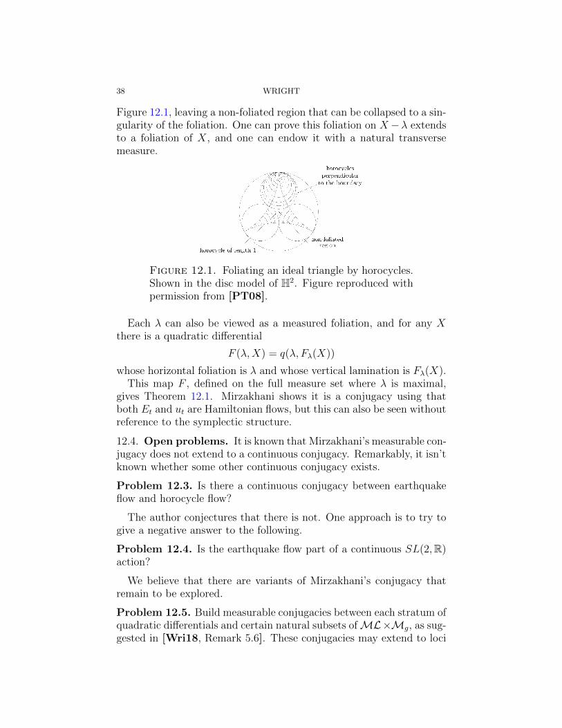
38 WRIGHT

Figure 12.1, leaving a non-foliated region that can be collapsed to a sin-gularity of the foliation. One can prove this foliation on X−λ extendsto a foliation of X, and one can endow it with a natural transversemeasure.

Figure 12.1. Foliating an ideal triangle by horocycles.Shown in the disc model of H2. Figure reproduced withpermission from [PT08].

Each λ can also be viewed as a measured foliation, and for any Xthere is a quadratic differential

F (λ,X) = q(λ, Fλ(X))

whose horizontal foliation is λ and whose vertical lamination is Fλ(X).This map F , defined on the full measure set where λ is maximal,

gives Theorem 12.1. Mirzakhani shows it is a conjugacy using thatboth Et and ut are Hamiltonian flows, but this can also be seen withoutreference to the symplectic structure.

12.4. Open problems. It is known that Mirzakhani’s measurable con-jugacy does not extend to a continuous conjugacy. Remarkably, it isn’tknown whether some other continuous conjugacy exists.

Problem 12.3. Is there a continuous conjugacy between earthquakeflow and horocycle flow?

The author conjectures that there is not. One approach is to try togive a negative answer to the following.

Problem 12.4. Is the earthquake flow part of a continuous SL(2,R)action?

We believe that there are variants of Mirzakhani’s conjugacy thatremain to be explored.

Problem 12.5. Build measurable conjugacies between each stratum ofquadratic differentials and certain natural subsets ofML×Mg, as sug-gested in [Wri18, Remark 5.6]. These conjugacies may extend to loci

MIRZAKHANI’S WORK ON RIEMANN SURFACES 39

of quadratic differentials with horizontal saddle connections betweenthe zeros.

Problem 12.6. Can some version of the horocyclic foliation Fλ bedefined for arbitrary non-maximal λ?

Yi Huang suggested that one might try to define Fλ so that its leavescontain the level sets of the nearest point projection to λ. (This projec-tion isn’t defined on the geodesic graph of points with more than oneclosest point on λ. See [Do08, Section 3.2] for some relevant results.)

13. Horocyclic measures

In this section we give an overview of the papers [LM08] and [Mir07a],which give somewhat related results concerning Teichmuller unipotentflow ut and earthquake flow Et respectively.

13.1. Warm up. We begin by explaining the theorem of Masur thatwas used in Section 9, in order to illustrate how the action of themapping class group onMF can be related to the action of unipotentflow on Q1Mg,n.

Theorem 13.1. The action of the mapping class group on MF isergodic with respect to the Thurston measure µTh.

This means that any invariant measure ν that is absolutely contin-uous with respect to µTh is a multiple of µTh.

Consider any mapping class group invariant measure ν onMF . De-fine a measure ν on the bundle of quadratic differentials Q1Tg,n, implic-itly using the isomorphism betweenQ1Tg,n and a subset ofMF ×MF ,by

ν(A) = ν × µTh({tq : q ∈ A, 0 < t < 1}),

for any A ⊂ Q1Tg,n. This ν has two important properties: it is MCG-invariant, and it is ut-invariant. The ut-invariance is very importantand not hard to prove, but won’t be obvious to non-experts.

The Masur-Veech measure on Q1Tg,n is µTh. It is the pull-back ofthe Masur-Veech measure on Q1Mg,n. Recall that the ut action onQ1Mg,n is ergodic.

If ν is absolutely continuous with respect to µTh, then ν is absolutelycontinuous with respect to µTh. One can show that the ergodicity ofthe ut action on Q1Mg,n implies that ν = cµTh for some c > 0, andthat that implies ν = cµTh.

40 WRIGHT

13.2. Ergodic theory on MF . Mirzakhani and Lindenstrauss clas-sified mapping class group invariant locally finite ergodic measures µon MF . To do so, they used that µ is not just ut-invariant, but it isalso horospherical, roughly meaning that it can be studied using themixing of geodesic flow gt. This connection to mixing is complicatedhere due to the non-compactness of Q1Mg, but this difficulty can beovercome by extending the quantitative non-divergence results for theut action proven in [MW02].

For any subsurface R, there is a natural inclusion

IR :MF(R)→MFfrom the spaceMF(R) of measured foliations on the subsurface to thespace of measured foliations on the whole surface. If R is bounded byclosed curves γ1, . . . , γk, then for any c = (c1, . . . , ck) ∈ Rk

+ Mirzakhaniand Lindenstrauss consider the map IcR :MF(R)→MF defined by

IcR(α) = IR(α) +∑

ciγi.

If µRTh is the Thurston measure on MF(R), Mirzakhani and Linden-strauss observe that (IcR)∗(µ

RTh) is a locally finite ergodic measure on

MF invariant under the mapping class group of S. Summing overcosets of the mapping class group of S in the mapping class group ofthe full surface gives a measure

µR,cTh =∑[g]

g∗(IcR(α))

that is still locally finite and ergodic, but is now invariant under thewhole mapping class group.

Mirzakhani and Lindenstrauss prove that every MCG-invariant lo-cally finite ergodic measure on MF is a multiple of µTh or µR,cTh forsome c and R. The same result was obtained in [Ham09].

13.3. Horospherical measures and earthquake flow. We now dis-cuss the results of [Mir07a]. There is a natural map

Mg−1,2(L,L)× R/(LZ)→Mg

obtained by gluing together the two boundary components with a twistgiven by an element of R/(LZ). Mirzakhani considers the push-forwardof Weil-Petersson measure onMg−1,2(L,L) times Lebesgue measure onR/(LZ), normalized to be a probability measure. She insightfully callsthese measures horospherical, but any direct analogy to horosphericalmeasures in other situations remains to be clarified, and her study doesnot use mixing or any analogue of the flow gt. Thus the terminologyshould not be taken literally.

MIRZAKHANI’S WORK ON RIEMANN SURFACES 41

She shows4 that these measures converge as L → ∞ to a proba-bility measure that is absolutely continuous with respect to the Weil-Petersson measure and has density B(X)/bg, a function that has al-ready appeared in Sections 9 and 12. This measure is the push-forwardvia (X,λ) 7→ X of the natural measure on P1Mg that is invariant underthe earthquake flow.

The map Mg−1,2(L,L) × R/(LZ) →Mg can be lifted to the set ofpairs (X, γ), where γ is the curve obtained from gluing the two bound-ary components. We can view γ/`γ(X) as a unit length measuredlamination on X, and in this way lift the map to the bundle P1Mg

of unit length measured laminations. Mirzakhani uses counting resultsto show that, in this space, any limit as L → ∞ of the push-forwardmeasures is absolutely continuous with respect to the natural earth-quake flow invariant measure. Any limit must also be invariant underearthquake flow, so she is then able to use ergodicity of earthquakeflow to identify such limit measures up to scale. She then uses non-divergence results from [MW02] to show that every limit as L → ∞is a probability measure, that is, that there is no loss of mass. Thisconcludes the proof that the pushfoward measures converge as L→∞to the natural invariant measure on P1Mg.

Other natural methods of building random surfaces in Mg are ex-pected to also equidistribute to B(X) times Weil-Petersson. For ex-ample, Bainbridge and Rafi informed the author that Mirzakhani ad-vertised the following question.

Problem 13.2. Fix a pants decomposition of a genus g surface. Foreach L, there is a torus inMg obtained by taking each cuff to be lengthL and looking at all possible twists. Show that these tori equidistributetowards B(X) times Weil-Petersson as L→∞.

However, random surfaces with respect to this measure are not yetwell-understood.

Problem 13.3. Study random surfaces in Mg sampled with respectto B(X) times the Weil-Petersson measure. For example, what are theasymptotics for the probability that a random surface has a geodesicof length at most ε, as g →∞?

4The author and others have not succeeded in understanding the proof of[Mir07a, Theorem 5.5(b)], however Francisco Arana Herrera has given an alter-nate proof of [Mir07a, Theorem 5.5(b)]. This is a key step in the proof that thelimit measures are absolutely continuous.

42 WRIGHT

14. Counting with respect to the Teichmuller metric

In his thesis [Mar04], Margulis considered a compact negativelycurved manifold M = M/Γ with universal cover M and fundamentalgroup π1(M) = Γ. For any X, Y ∈ M , he proved the asymptotic

|Γ · Y ∩BR(X)| ∼ cX,Y ehR

for the number of points in the orbit Γ · Y in the ball BR(X), whereh > 0 is the topological entropy of the geodesic flow, and cX,Y > 0 is aconstant depending on X and Y . This is called a “lattice point count”,since one thinks of the orbit Γ · y analogously to an orbit of Zk actingon Rk. He also showed that the number of primitive oriented closed

geodesics of length less than R is asymptotic to ehR

hR.

Instead of such M , we wish to consider Mg equipped with the Te-ichmuller metric. In comparing Mg to a compact negatively curvedmanifold, one should note the following points.

• The Teichmuller metric has some features of negative curvature,and is even negatively curved “on average” [DDM14].• It is however not actually negatively curved in any sense. For

example, there are pairs of infinite geodesic rays in Tg leavingthe same point that stay bounded distance apart [Mas75].• There exist closed geodesics outside of any given compact subset

of Mg.

Despite these major differences, Mirzakhani and her coauthors ob-tained results forMg analogous to those Margulis obtained for compactnegatively curved manifolds [ABEM12,EM11,EMR19].

14.1. Lattice point counting. Consider the action of Γ = MCG onTg, and consider balls BR(Y ) of radius R centered at Y ∈ Tg. Athreya,Bufetov, Eskin, and Mirzakhani proved the following.

Theorem 14.1. As R→∞,

|Γ · Y ∩BR(X)| ∼ CX,Y ehR,

where h = 6g − 6 is the entropy of the Teichmuller geodesic flow andCX,Y is an explicit constant.

Dumas and Mirzakhani later discovered that the constant CX,Y doesnot depend on the choice of X, Y ∈ Tg [Dum15, Theorem 5.10]. Itwould be interesting to understand the asymptotics of this constant asg →∞.

In comparison to the problem of counting points in Zk in a ball, thedifficulty of this problem is that most of the points of Γ ·Y ∩BR(X) lie

MIRZAKHANI’S WORK ON RIEMANN SURFACES 43

near the boundary sphere of BR(X); this is witnessed by the exponen-tial growth of the count. A solution is to use mixing of the gt action toprove that large spheres are equidistributed in Mg, and to apply thisequidistribution to understand how many points of Γ · Y each concen-tric sphere of BR(X) is close to. For an introduction to this techniquein the simplest situation, we highly recommend [EM93, Section 2]. Inthis situation, a key technical issue is the smaller dimensional strata ofthe bundle of quadratic differentials, close to which the flow gt is lessunderstood.

Athreya, Bufetov, Eskin, and Mirzakhani also give asymptotics forthe volume of BR(X).

14.2. Counting closed orbits. Let N(R) denote the number of prim-itive oriented closed geodesics on Mg of length at most R.

Following Thurston, every element of the mapping class group canbe classified as periodic, reducible, or pseudo-Anosov [FM12, Chapter13]. Briefly, an element is pseudo-Anosov if none of its powers fix amulti-curve; these elements are thought of as “generic” in the mappingclass group.

Conjugacy classes of pseudo-Anosovs are in bijection with orientedclosed geodesics on Mg, and the translation length of the pseudo-Anosov acting on Tg is the length of the closed geodesic. Thus, N(R)can also be interpreted as the number of conjugacy classes of primitivepseudo-Anosovs of translation length at most R.

Eskin and Mirzakhani show the following.

Theorem 14.2. As R→∞,

N(R) ∼ ehR

hR.

Later, Eskin, Mirzakhani and Rafi proved a version of this for the gtaction on individual strata of quadratic differentials.

The basic idea of the proof is to use mixing of the gt action to countthe number of orbit segments of gt that come back close to where theystarted, and to prove a Closing Lemma to show that typically eachsuch orbit segment lies close to a closed orbit. Following a standardargument, the Closing Lemma is deduced from two applications of thecontraction mapping principle and the hyperbolicity results discussedin Section 11.7.

This strategy, however, only gives information on the closed geodesicsthat intersect some fixed compact set inMg. AndMg contains a greatmany closed geodesics outside of any compact set [Ham16].

44 WRIGHT

The key to counting closed geodesics in this context is thus to showthat there are not too many that live entirely outside a compact set.More precisely, if K is a large compact set, the authors show that thenumber of closed geodesics of length R that stay outside of K has asmaller exponential order of growth than N(R).

To prove this, the authors consider a discretization of a geodesicinto a sequence of bounded length segments between a discrete “net”of points in Tg. They then show that most such sequence do not avoida compact set. In a precise sense, a random sequence is biased towardsreturning to compact sets, and so it is very unlikely that a long randomsequence entirely avoids a fixed large compact set.

This final step is more difficult in the case of strata, and in fact theproblem is open in a more general context discussed in Section 16.

Problem 14.3. Prove a version of Theorem 14.2 that counts closed gtorbits in a SL(2,R)–orbit closure in a stratum.

15. From orbits of curves to orbits in Teichmuller space

In Mirzakhani’s proof of Theorem 9.1, discussed in Section 9, it wasabsolutely crucial that γ be a simple multi-curve, so that it defines apoint of MF , and so that the integration formula can be applied. Inone of her most recent papers, which is supplemented by forthcomingwork of Rafi and Souto, Mirzakhani gave a totally different approachto this problem that allowed for γ to have self-intersections [Mir16].

Theorem 15.1. Let γ be any homotopy class of closed curve.5 Then

limL→∞

sX(L, γ)

L6g−6+2n=c(γ) ·B(X)

bg,n,

where B(X) = µTh(BX) and bg,n =∫B(X) dVolWP are as in Sections

9 and 12 and c(γ) ∈ Q+.

For any k, the set of curves with exactly k self-intersections is a finiteunion of mapping class group orbits, so this result implies asymptoticsfor the set of curves with k self-intersections. In the case of a oncepunctured torus, this result can be used to count integer solutions tothe Markoff equation p2 + q2 + r2 = 3pqr [Mir16, Section 3].

In forthcoming work, Erlandsson and Souto will give an independentproof of Theorem 15.1.

5Most of [Mir16] is devoted to the case of filling curves. Mirzakhani claims thatthe non-filling case is similar, referring in the last paragraph of the proof of Theorem1.1 to a remark in Section 6.3. That remark seems incorrect. In forthcoming work,Rafi and Souto explain how to deduce the non-filling case from the filling case [RS].

MIRZAKHANI’S WORK ON RIEMANN SURFACES 45

15.1. Other notions of length. In the same way that each simpleclosed curve defines a point in MF , each closed curve defines a pointin the space C of geodesic currents. You can think of this space as acompletion of the space of linear combinations of closed curves, in thesame way thatMF is a completion of the space of linear combinationsof simple multi-curves.

One can define the length on X of any current; this is uniquely spec-ified by the fact that the length function C → R+ is continuous. Moregenerally, one could consider any reasonably nice function f : C → R+

as defining a type of length on currents. There are numerous importantexamples of such functions f , including length on a fixed Riemannianmetric with negative but non-constant curvature, and notions of lengthcoming from Higher Teichmuller Theory.

A combination of Mirzakhani’s result and work of Erlandsson andSouto give that Theorem 15.1 is true even if we replace sX(L, γ) with

sf (L, γ) = |{α ∈ MCG ·γ : f(α) ≤ L}| ,

for any homogeneous and continuous f : C → R+ [ES16]. Roughlyspeaking, Erlandsson and Souto show that the problem of countingsf (L, γ) does not depend on which f is used, and Theorem 15.1 solvesthis problem when f is the usual length on some hyperbolic surface X.

Rafi and Souto additionally showed that one can count mapping classgroup orbits of more general currents, and also identified Mirzakhani’sconstant c(γ) [RS17]. See [EU18] for a survey of related develop-ments.

15.2. The idea of the proof. Take γ a filling curve. By definition,this means that γ intersects every simple closed curve.

Mirzakhani transforms the problem to a counting problem on Te-ichmuller space. First, she observes that Stab(γ) is finite and

sX(L, γ) =|{g ∈ MCG : `X(g · γ) ≤ L}|

|Stab(γ)|.

But `X(g · γ) = `g−1·X(γ), and Stab(X) is finite for any X, so we get

|{g ∈ MCG : `X(g · γ) ≤ L}|= |{g ∈ MCG : `g·X(γ) ≤ L}|= |Stab(X)| · |{Y ∈ MCG ·X : `Y (γ) ≤ L}| .

In summary, the problem is reduced to counting the number of elementsin the mapping class group orbit of X that lie in the compact set

Bγ(L) = {Y ∈ Tg,n : `γ(Y ) ≤ L}.

46 WRIGHT

This problem is similar to the lattice point count of the previous section,except that the shape of the set Bγ(L) is a priori not as well understood.

Mirzakhani shows that in Fenchel-Nielsen coordinates, Bγ(L) isn’ttoo strangely shaped: it is asymptotically polyhedral. In the previouslattice point counting problem, Mirzakhani and her coauthors usedequidistribution of certain spheres in Mg. Similarly, here Mirzakhaniuses that the boundary of Bγ(L) equidistributes in moduli space asL → ∞. She does this by showing that the boundary can be dividedinto pieces that can be approximated by pieces of “horospheres” similarto those studied in Section 12.3, and using equidistribution of those“horospheres”.

16. SL(2,R)–invariant measures and orbit closures

McMullen classified SL(2,R)-invariant measures and orbit closuresof Abelian differentials in genus 2 [McM07], and Mirzakhani wasdeeply interested in generalizing these results to higher genus. In thissection, we discuss the results from [EM18, EMM15] on this topic.Lectures notes of Eskin, a short survey by the author, and an in-depthsurvey by Quint all give more details [Esk,Wri16,Qui16].

First, Eskin and Mirzakhani understood

P =

{(∗ ∗0 ∗

)}⊂ SL(2,R)

invariant measures on moduli spaces of translation surfaces.

Theorem 16.1. Every P -invariant ergodic probability measure on thelocus of unit area surfaces in a stratum is the natural Lebesgue measureon the unit area locus of a (properly immersed) linear sub-orbifold ofthe stratum. In particular, it is SL(2,R)-invariant.

A sub-orbifold is linear if it is locally described by linear equationson the edges of polygons defining the surfaces, and if these equationshave zero constant term and real coefficients.

Then, Eskin, Mirzakhani and Mohammadi used the previous resultto prove the following.

Theorem 16.2. The P -orbit closure of any point is equal to the SL(2,R)-orbit closure of that point, and is the unit area locus of a linear sub-orbifold of the stratum.

Before giving the definitions, we give some of the reasons why somuch interest has focused on these questions, and why these theoremshave been called a “Magic Wand” for applications [Zor14,Zor15].

MIRZAKHANI’S WORK ON RIEMANN SURFACES 47

• Since each SL(2,R) orbit projects to a complex geodesic inMg,n, orbit closures are related to the geometry of Mg,n.• Quadratic differentials arise naturally in the study of billiards in

rational polygons. Questions such as the number of generalizeddiagonals in a polygon can be productively studied using, andin fact depend on, the SL(2,R) orbit closure.• There are applications to other simplified models in physics,

such as the Ehrenfest Wind Tree Model and periodic arrays ofEaton lenses [FSU18].• There are applications to other low complexity dynamical sys-

tems such as interval exchange transformations and flows onsurfaces, as well as the illumination problem [LMW16]. (Ifthe edges of a non-convex polygon were reflective, what subsetof the polygon would be illuminated by a light source in thepolygon?)• The orbit closures turn out to be beautiful and independently

interesting algebraic varieties.• The are deep connections to homogeneous space dynamics, which

have enriched both fields.

Each point of the SL(2,R)-orbit of a surface (X, q) represents adifferent perspective on (X, q), which in a sense arises from a linearchange of coordinates. Understanding the orbit of a surface representsunderstanding all possible perspectives on the surface simultaneously.

16.1. Definitions. We begin with a warm up observation. Considerthe diagonal action of GL(2,R) on Cm ' (R2)m. A subspace of Cm

is invariant under this action if and only if it can be cut out by linearequations with real coefficients. This explains the definition of linearsubmanifold. It is almost as easy to see that a linear submanifold ofa stratum must be invariant by GL(2,R), since this can be checkedlocally.

Each linear submanifold M inherits from the stratum an atlas ofcharts to Cm with transition functions in GL(m,R). Suppose the tran-sition functions can be chosen to have determinant ±1. For Theorem16.1 it suffices to deal with this case, and actually it turns out this isalways possible. Then there is a natural Lebesgue µ measure on M,well-defined up to scale. From this, one can define a measure µ1 on theunit area locus by

µ1(A) = µ({t(X,ω) : t ∈ (0, 1), (X,ω) ∈ A}).

It is exactly these measures that we refer to in Theorem 16.1.

48 WRIGHT

16.2. Previous results in measure rigidity. Theorems 16.1 and16.2 were inspired by and built upon related results in homogeneousspace dynamics, where one considers group actions on homogeneousspaces rather than moduli spaces of surfaces.

The philosophy behind this line of work is that, even if one wants pri-marily to understand orbit closures, it is more convenient to first workwith invariant measures. For a short introduction to this philosophy,see Venkatesh’s survey [Ven08].

Any student seriously interested in learning the proofs of Theorems16.1 and 16.2 might be well advised to start in the homogeneous set-ting, for example by reading about Ratner’s Theorems from expositorysources such as [Ein06, Esk10, Mor05], or by reading the work ofBenoist and Quint [BQ11, BQ+16]. Let us briefly mention the workof Benoist and Quint in the simplest example.

Theorem 16.3. Let µ be a finitely supported measure on SL(2,Z). Ifν is any non-atomic µ-stationary probability measure on R2/Z2, thenν is Lebesgue.

Here SL(2,Z) acts on the torus R2/Z2 in the usual way, and ν iscalled µ-stationary if it is “invariant on average” by the SL(2,Z) action:

ν =∑

g∈SL(2,Z)

µ(g)g∗ν.

In particular, every invariant measure is stationary, but there aremany important situations where one cannot prove the existence ofinvariant measures but can easily show that stationary measures exist.Stationary measures are closely related to the study of random walks.

Using Theorem 16.3, Benoist and Quint are able to also understandorbit closures, and show that any closed set invariant under SL(2,Z)must be finite or the whole torus R2/Z2.

In addition to the ideas of Ratner, Benoist, and Quint, and newideas, Eskin and Mirzakhani make use of ideas developed in the con-text of homogeneous dynamics by mathematicians including Margulis,Tomanov, Einsiedler, Katok, and Lindenstrauss [MT94,EKL06].

16.3. Structure of the proofs. The techniques used by Eskin, Mirza-khani, and Mohammadi are very abstract, and do not directly involvethe geometry of surfaces.

Instead, Eskin and Mirzakhani focus on entropy and the rates atwhich the geodesic flow gt expands and contracts. These rates are calledLyapunov exponents, and are the subject of work of Forni and others inthis context [FM14]. They also use an idea of Furstenburg to convert

MIRZAKHANI’S WORK ON RIEMANN SURFACES 49

the problem about P -invariant measures to a problem about measuresthat are stationary with respect to certain measures on SL(2,R).

The hardest and longest part of the proof of Theorem 16.1 works inthis framework to prove that a stationary measure is in fact SL(2,R)-invariant. Once the measure is known to be SL(2,R)-invariant, Eskinand Mirzakhani use a version of the arguments of Benoist and Quint toconclude. The general framework of the proof is to establish additionalinvariance properties bit by bit, but this is complicated by the fact thathere the additional “invariance” is often not given by a global actionof a group.

The algebraic properties of P , namely that it is amenable, allow Es-kin, Mirzakhani and Mohammadi to “average” over partial P -orbits toconstruct, from each P -orbit, a P -invariant measure. This would notbe possible with SL(2,R), and is the chief reason that Eskin and Mirza-khani worked so hard to understand P -invariant measures, instead ofthe easier SL(2,R)-invariant measures.

Eskin, Mirzakhani and Mohammadi show that the support of themeasure constructed from each orbit is equal to that orbit closure, andin this way prove Theorem 16.2.

16.4. Subsequent work and open problems. The techniques of[EM18,EMM15] have since been applied to homogeneous and smoothdynamics [ELb,ELa,BRH17].

Mirzakhani was deeply interested in the ut action.

Problem 16.4. Understand ut-invariant measures and orbit closures.

The hope was originally for a version of Ratner’s Theorems in thiscontext. However, a recent discovery of Chaika, Smillie and Weissshows that ut-orbit closures can have non-integral Hausdorff dimension,so the theory for homogeneous spaces cannot hold in full in this context[CSW]. However, one can still hope for progress for particular classesof ut-invariant measures.

Problem 16.5. Understand piecewise linear ut-invariant measures andorbit closures.

We conclude with a question recommended to us by McMullen, con-cerning a generalization of flat surfaces arising by tensoring the bundleof quadratic differentials on a Riemann surface with a flat line bundlewith holonomy in R+.

Problem 16.6. What can one say about the action of SL2(R) onbundles Q′Mg →Mg of twisted quadratic differentials?

50 WRIGHT

Twisted quadratic differentials are examples of dilation surfaces,whose moduli spaces may have features in common with infinite vol-ume hyperbolic manifolds. See [Gha18, Section 8] more details, aswell as for some conjectures and open problems.

17. Classification of SL(2,R)–orbit closures

It turns out that orbit closures of translation surfaces are varietiesthat can be characterized by unlikely algebro-geometric properties [Fil16],and there are at most countably many of them. Mirzakhani proposedthe following in answer to the mystery of why so few examples of orbitclosures are known.

Conjecture 17.1. Every orbit closure of rank at least 2 is trivial.

We define these terms for orbit GL+(2,R)–orbit closures of Abeliandifferentials. One can get corresponding definitions for orbit closuresof quadratic differentials by passing to double covers where the qua-dratic differentials are squares of Abelian differentials. The change fromSL(2,R) to GL+(2,R) is unimportant but simplifies the notation.

The tangent space T(X,ω)M to an orbit closure M of Abelian dif-ferentials is naturally a subspace of the relative cohomology groupH1(X,Σ,C), where Σ is the set of zeros of ω. There is a naturalmap p : H1(X,Σ,C)→ H1(X,C), and

rank(M) =1

2dimC p(T(X,ω)M)

for any (X,ω) ∈M. This is an integer between 1 and the genus of X.

Example 17.2. The rank of a closed orbit is 1. The rank of a stratumof genus g Abelian differentials is g.

An alternative definition of rank is provided by Filip’s work: Thereis a number field k(M) that acts naturally on the space H1,0(X,C)of Abelian differentials for each (X,ω) ∈ M. (In fact k(M) is totallyreal, and the action comes from an action on Jac(X).) The cohomologyclass of ω is a eigenvector for this action, and the rank is the dimensionof the eigenspace.

An orbit closure is called trivial if it arises via a branched coveringconstruction from a stratum of Abelian or quadratic differentials.

Example 17.3. Consider a connected component M of the locus of(X,ω) for which there exists a (X ′, ω′) ∈ H(2) and degree 3 coverf : X → X ′, simply branched over one point that isn’t a zero of ω′,such that ω = f ∗(ω′). ThisM is trivial, since it arises from H(2) from

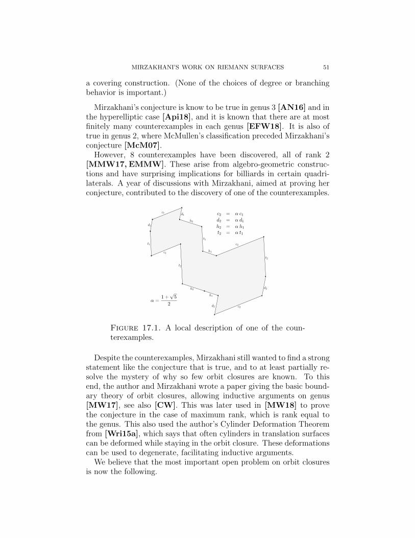
MIRZAKHANI’S WORK ON RIEMANN SURFACES 51

a covering construction. (None of the choices of degree or branchingbehavior is important.)

Mirzakhani’s conjecture is know to be true in genus 3 [AN16] and inthe hyperelliptic case [Api18], and it is known that there are at mostfinitely many counterexamples in each genus [EFW18]. It is also oftrue in genus 2, where McMullen’s classification preceded Mirzakhani’sconjecture [McM07].

However, 8 counterexamples have been discovered, all of rank 2[MMW17, EMMW]. These arise from algebro-geometric construc-tions and have surprising implications for billiards in certain quadri-laterals. A year of discussions with Mirzakhani, aimed at proving herconjecture, contributed to the discovery of one of the counterexamples.

Figure 17.1. A local description of one of the coun-terexamples.

Despite the counterexamples, Mirzakhani still wanted to find a strongstatement like the conjecture that is true, and to at least partially re-solve the mystery of why so few orbit closures are known. To thisend, the author and Mirzakhani wrote a paper giving the basic bound-ary theory of orbit closures, allowing inductive arguments on genus[MW17], see also [CW]. This was later used in [MW18] to provethe conjecture in the case of maximum rank, which is rank equal tothe genus. This also used the author’s Cylinder Deformation Theoremfrom [Wri15a], which says that often cylinders in translation surfacescan be deformed while staying in the orbit closure. These deformationscan be used to degenerate, facilitating inductive arguments.

We believe that the most important open problem on orbit closuresis now the following.

52 WRIGHT

Problem 17.4. Is every orbit closure of rank at least 3 trivial?

Some limited theoretical and computer efforts have failed to find anynon-trivial orbit closures of rank at least 3 thus far. Furthermore, every(X,ω) with a rank 2 orbit closure has a natural map X → P1, whichplayed a crucial role in the 8 counterexamples. However, in the rank3 case there is instead a map X → P2, and so far there is no proposalfor how this map could be leveraged to establish the special algebro-geometric properties that, by the work of Filip, must be present.

There are myriad other open problems about orbit closures, but weconclude by mentioning just two that Mirzakhani was interested in.

Problem 17.5. Give an effective proof that there are only finitelymany orbit closures of rank at least 2 in each genus.

Problem 17.6. Classify algebraically primitive orbit closures of rankat least 2, where an orbit closure is algebraically primitive if rank(M) ·[k(M) : Q] = g. Start with the case where k(M) is quadratic.

See [Wri15b] for the author’s more in depth (although now some-what out of date) survey aimed towards orbit closures, and see [MW18]for a few additional open problems.

18. Effective counting of simple closed curves

We now discuss work of Eskin, Mirzakhani, and Mohammadi thatgives an effective version of Theorem 9.1 with a totally different proof[EMM10]. Recall that if X is a hyperbolic surface and γ is a multi-curve,

sX(L, γ) = |{α ∈ MCG ·γ : `α(X) ≤ L}|.

Theorem 18.1. There is a constant κ = κ(g) > 0 such that for anyX ∈Mg and any rational multi-curve γ,

sX(L, γ) =c(γ) ·B(X)

bgL6g−6 +O(L6g−6−κ).

Here the constants c(γ), B(X), bg are as in Theorem 9.1, but will notplay a major role in our discussion.

The proof of Theorem 18.1 uses the dynamics of Teichmuller geodesicsflow, and the effective nature of the count comes from the exponentialmixing of this flow proven in [AGY06].

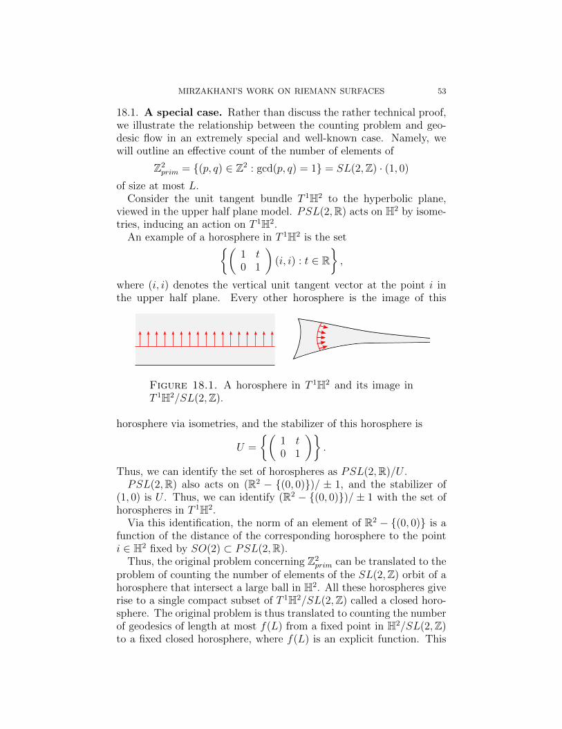
MIRZAKHANI’S WORK ON RIEMANN SURFACES 53

18.1. A special case. Rather than discuss the rather technical proof,we illustrate the relationship between the counting problem and geo-desic flow in an extremely special and well-known case. Namely, wewill outline an effective count of the number of elements of

Z2prim = {(p, q) ∈ Z2 : gcd(p, q) = 1} = SL(2,Z) · (1, 0)

of size at most L.Consider the unit tangent bundle T 1H2 to the hyperbolic plane,

viewed in the upper half plane model. PSL(2,R) acts on H2 by isome-tries, inducing an action on T 1H2.

An example of a horosphere in T 1H2 is the set{(1 t0 1

)(i, i) : t ∈ R

},

where (i, i) denotes the vertical unit tangent vector at the point i inthe upper half plane. Every other horosphere is the image of this

Figure 18.1. A horosphere in T 1H2 and its image inT 1H2/SL(2,Z).

horosphere via isometries, and the stabilizer of this horosphere is

U =

{(1 t0 1

)}.

Thus, we can identify the set of horospheres as PSL(2,R)/U .PSL(2,R) also acts on (R2 − {(0, 0)})/ ± 1, and the stabilizer of

(1, 0) is U . Thus, we can identify (R2 − {(0, 0)})/ ± 1 with the set ofhorospheres in T 1H2.

Via this identification, the norm of an element of R2 − {(0, 0)} is afunction of the distance of the corresponding horosphere to the pointi ∈ H2 fixed by SO(2) ⊂ PSL(2,R).

Thus, the original problem concerning Z2prim can be translated to the

problem of counting the number of elements of the SL(2,Z) orbit of ahorosphere that intersect a large ball in H2. All these horospheres giverise to a single compact subset of T 1H2/SL(2,Z) called a closed horo-sphere. The original problem is thus translated to counting the numberof geodesics of length at most f(L) from a fixed point in H2/SL(2,Z)to a fixed closed horosphere, where f(L) is an explicit function. This

54 WRIGHT

problem manifestly involves geodesic flow, and ideas of Margulis canbe used to solve it effectively.

18.2. The hyperbolic length function. The above outline could beused to count elements of Z2

prim of “size” at most L, where the notionof “size” is given by a sufficiently nice function.

Similarly, Eskin-Mirzakhani-Mohammadi must check that their no-tion of “size” is sufficiently nice. They do this with a result from Mirza-khani’s thesis [Mir04, Theorem A.1], which states that the hyperboliclength function

α 7→ `α(X)

is a convex function on natural subsets ofML called train track charts.A corollary is that this function is Lipschitz.

We end with the natural next step in this line of investigation.

Problem 18.2. Generalize Theorem 18.1 to non-simple multi-curves,thus giving an effective version of Theorem 15.1.

19. Random walks on the mapping class group

Consider a reasonably nice measure µ on the group of isometriesof H2. One of the archetypal features of negative curvature is that arandom walk on H2 with steps determined by µ will converge almostsurely to the circle ∂H2 at infinity.

If one fixes a starting point, there is a “hitting measure” ν on ∂H2,whose defining property is that the measure ν(A) of any subset A ⊂∂H2 is equal to the probability that a random walk path will convergeto a point in A. The hitting measure is also sometimes called theharmonic measure, because it satisfies an equation saying that it isunchanged by averaging over µ. If the support of µ is discrete, thisequation can be written as

(19.0.1) ν =∑γ

µ(γ)γ∗(ν).

Moreover, almost every random walk path tracks a geodesic ray,and the endpoint of the geodesic ray is the point in ∂H2 that therandom walk path converges to. More precisely, the geometric form ofthe Oseledets Multiplicative Ergodic Theorem states that the distancebetween the the random walk path and the geodesic ray that it tracksis sub-linear in the number of steps of the random walk.

A natural way to pick a random geodesic ray leaving a point is tosimply pick the endpoint of the ray using the Lebesgue measure on thecircle. This notion captures what is commonly understood as a randomgeodesic ray.

MIRZAKHANI’S WORK ON RIEMANN SURFACES 55

One may ask: How different are random geodesic rays and randomwalk paths? Can one simulate the effect of picking a random geodesicray by instead generating a random walk path? This question has extrasignificance if we want the the measure µ defining the random walk tolive in a discrete subgroup such as SL(2,Z). Can one simulate a ran-dom geodesic ray on H2/SL(2,Z) by a random walk on its fundamentalgroup SL(2,Z)?

At first, this seems like a lot to ask for. Indeed, although the geodesicflow on the unit tangent bundle T 1H2/SL(2,Z) is very chaotic, it is ofcourse a deterministic process. In contrast, the random walk has no“memory” at all, in that each step of the random walk does not dependat all on the previous steps. For this reason, random walks are easierto study than the geodesic flow.

Nonetheless, Furstenberg famously proved that one can simulate therandom geodesic ray with a random walk path: There is a measureon SL(2,Z) whose hitting measure on ∂H2 is Lebesgue. Furstenbergobtained his measure µ as a discretization of Brownian motion, andused it to prove one of the first rigidity results, for example that groupslike SL(n,Z), n > 2 cannot be isomorphic to subgroups of SL(2,R).For a very clear exposition, see [Fur71, Sections 5, 6].

In forthcoming work, Eskin, Mirzakhani and Rafi will give an ana-logue of Furstenberg’s result in the context of Teichmuller theory [EMR].Thus H2 will be replaced with Teichmuller space, and the circle ∂H2 atinfinity will be replaced with the Thurston boundary of Teichmullerspace. In this context the hitting measure is defined via work ofKaimanovich and Masur [KM96].

Eskin, Mirzakhani and Rafi follow an approach of Connell and Much-nik, who generalized Furstenberg’s results to apply, for example, tocompact manifolds of negative curvature [CM07]. Instead of usingBrownian motion, this approach pursues a more direct method for solv-ing Equation (19.0.1).

References

[ABEM12] Jayadev Athreya, Alexander Bufetov, Alex Eskin, and Maryam Mirza-khani, Lattice point asymptotics and volume growth on Teichmullerspace, Duke Math. J. 161 (2012), no. 6, 1055–1111.

[AGY06] Artur Avila, Sebastien Gouezel, and Jean-Christophe Yoccoz, Exponen-

tial mixing for the Teichmuller flow, Publ. Math. Inst. Hautes EtudesSci. (2006), no. 104, 143–211.

[AH19] Francisco Arana-Herrera, Counting square-tiled surfaces with prescribedreal and imaginary foliations and connections to Mirzakhani’s asymp-totics for simple closed hyperbolic geodesics, arXiv:1902.05626 (2019).

56 WRIGHT

[AN16] David Aulicino and Duc-Manh Nguyen, Rank two affine manifolds ingenus 3, arXiv:1612.06970 (2016).

[Api18] Paul Apisa, GL2R orbit closures in hyperelliptic components of strata,Duke Math. J. 167 (2018), no. 4, 679–742.

[BM00] M. Bachir Bekka and Matthias Mayer, Ergodic theory and topologicaldynamics of group actions on homogeneous spaces, London Mathemat-ical Society Lecture Note Series, vol. 269, Cambridge University Press,Cambridge, 2000.

[BM04] Robert Brooks and Eran Makover, Random construction of Riemannsurfaces, J. Differential Geom. 68 (2004), no. 1, 121–157.

[BQ11] Yves Benoist and Jean-Francois Quint, Mesures stationnaires et fermesinvariants des espaces homogenes, Ann. of Math. (2) 174 (2011), no. 2,1111–1162.

[BQ+16] Y Benoist, J-F Quint, et al., Translation of the paper “Mesures station-naires et fermes invariants des espaces homogenes”, by Y. Benoist andJ.-F. Quint, arXiv:1610.05912 (2016).

[BRH17] Aaron Brown and Federico Rodriguez Hertz, Measure rigidity for ran-dom dynamics on surfaces and related skew products, J. Amer. Math.Soc. 30 (2017), no. 4, 1055–1132.

[BS85] Joan S. Birman and Caroline Series, Geodesics with bounded intersec-tion number on surfaces are sparsely distributed, Topology 24 (1985),no. 2, 217–225.

[BS01] Francis Bonahon and Yasar Sozen, The Weil-Petersson and Thurstonsymplectic forms, Duke Math. J. 108 (2001), no. 3, 581–597.

[BT16] Martin Bridgeman and Ser Peow Tan, Identities on hyperbolic man-ifolds, Handbook of Teichmuller theory. Vol. V, IRMA Lect. Math.Theor. Phys., vol. 26, Eur. Math. Soc., Zurich, 2016, pp. 19–53.

[CdS01] Ana Cannas da Silva, Lectures on symplectic geometry, Lecture Notesin Mathematics, vol. 1764, Springer-Verlag, Berlin, 2001.

[CM07] Chris Connell and Roman Muchnik, Harmonicity of quasiconformalmeasures and Poisson boundaries of hyperbolic spaces, Geom. Funct.Anal. 17 (2007), no. 3, 707–769.

[CSW] Jon Chaika, John Smillie, and Barak Weiss, Tremors and horocycledynamics on the moduli space of translation surfaces, in preparation.

[CW] Dawei Chen and Alex Wright, The WYSIWYG compactification, inpreparation.

[DDM14] Spencer Dowdall, Moon Duchin, and Howard Masur, Statistical hyper-bolicity in Teichmuller space, Geom. Funct. Anal. 24 (2014), no. 3,748–795.

[DGZZ] Vincent Delecroix, Elise Goujard, Peter Zograf, and Anton Zorich,Square-tiled surfaces of fixed combinatorial type: equidistribution,counting, volumes of the ambient strata, in preparation.

[DN09] Norman Do and Paul Norbury, Weil-Petersson volumes and cone sur-faces, Geom. Dedicata 141 (2009), 93–107.

[Do08] Norman Nam Van Do, Intersection theory on moduli spaces of curvesvia hyperbolic geometry, Ph.D. thesis, 2008.

[Do10] Norman Do, The asymptotic weil-petersson form and intersection the-ory on Mg,n, arXiv:1010.4126 (2010).

MIRZAKHANI’S WORK ON RIEMANN SURFACES 57

[Do13] , Moduli spaces of hyperbolic surfaces and their Weil-Peterssonvolumes, Handbook of moduli. Vol. I, Adv. Lect. Math. (ALM), vol. 24,Int. Press, Somerville, MA, 2013, pp. 217–258.

[Dum15] David Dumas, Skinning maps are finite-to-one, Acta Math. 215 (2015),no. 1, 55–126.

[EFW18] Alex Eskin, Simion Filip, and Alex Wright, The algebraic hull of theKontsevich-Zorich cocycle, Ann. of Math. (2) 188 (2018), no. 1, 281–313.

[Ein06] Manfred Einsiedler, Ratner’s theorem on SL(2,R)-invariant measures,Jahresber. Deutsch. Math.-Verein. 108 (2006), no. 3, 143–164.

[EKL06] Manfred Einsiedler, Anatole Katok, and Elon Lindenstrauss, Invariantmeasures and the set of exceptions to Littlewood’s conjecture, Ann. ofMath. (2) 164 (2006), no. 2, 513–560.

[ELa] Alex Eskin and Elon Lindenstrauss, Random walks on llo-cally homogeneous spaces, https://www.math.uchicago.edu/~eskin/RandomWalks/paper.pdf.

[ELb] , Zariski dense random walks on homogeneous spaces, https:

//www.math.uchicago.edu/~eskin/RandomWalks/short_paper.pdf.[ELSV01] Torsten Ekedahl, Sergei Lando, Michael Shapiro, and Alek Vainshtein,

Hurwitz numbers and intersections on moduli spaces of curves, Invent.Math. 146 (2001), no. 2, 297–327.

[EM93] Alex Eskin and Curt McMullen, Mixing, counting, and equidistributionin Lie groups, Duke Math. J. 71 (1993), no. 1, 181–209.

[EM11] Alex Eskin and Maryam Mirzakhani, Counting closed geodesics in mod-uli space, J. Mod. Dyn. 5 (2011), no. 1, 71–105.

[EM18] , Invariant and stationary measures for the SL(2,R) action on

moduli space, Publ. Math. Inst. Hautes Etudes Sci. 127 (2018), 95–324.[EMM10] Alex Eskin, Maryam Mirzakhani, and Amir Mohammadi, Effec-

tive counting of simple closed geodesics on hyperbolic surfaces,arXiv:1905.04435 (2010).

[EMM15] , Isolation, equidistribution, and orbit closures for the SL(2,R)action on moduli space, Ann. of Math. (2) 182 (2015), no. 2, 673–721.

[EMMW] Alex Eskin, Curtis McMullen, Ronen Mukamel, and Alex Wright,Billiards, quadrilaterals and moduli spaces, http://www-personal.

umich.edu/~alexmw/dm.pdf.[EMR] Alex Eskin, Maryam Mirzakhani, and Kasra Rafi, forthcoming.[EMR19] , Counting closed geodesics in strata, Invent. Math. 215 (2019),

no. 2, 535–607.[ES16] Viveka Erlandsson and Juan Souto, Counting curves in hyperbolic sur-

faces, Geom. Funct. Anal. 26 (2016), no. 3, 729–777.[ES19] , Mirzakhani’s Curve Counting, arXiv:1904.05091 (2019).[Esk] Alex Eskin, Lectures on the SL(2,R) action on moduli space, https:

//www.math.uchicago.edu/~eskin/luminy2012/lectures.pdf.[Esk10] , Unipotent flows and applications, Homogeneous flows, moduli

spaces and arithmetic, Clay Math. Proc., vol. 10, Amer. Math. Soc.,Providence, RI, 2010, pp. 71–129.

[EU18] Viveka Erlandsson and Caglar Uyanik, Length functions on currentsand applications to dynamics and counting, arXiv:1803.10801 (2018).

58 WRIGHT

[Eyn14] Bertrand Eynard, A short overview of the “Topological recursion”,arXiv:1412.3286 (2014).

[Fil16] Simion Filip, Splitting mixed Hodge structures over affine invariantmanifolds, Ann. of Math. (2) 183 (2016), no. 2, 681–713.

[FM12] Benson Farb and Dan Margalit, A primer on mapping class groups,Princeton Mathematical Series, vol. 49, Princeton University Press,Princeton, NJ, 2012.

[FM14] Giovanni Forni and Carlos Matheus, Introduction to Teichmuller theoryand its applications to dynamics of interval exchange transformations,flows on surfaces and billiards, J. Mod. Dyn. 8 (2014), no. 3-4, 271–436.

[For02] Giovanni Forni, Deviation of ergodic averages for area-preserving flowson surfaces of higher genus, Ann. of Math. (2) 155 (2002), no. 1, 1–103.

[FSU18] Krzysztof Fraczek, Ronggang Shi, and Corinna Ulcigrai, Genericity oncurves and applications: pseudo-integrable billiards, Eaton lenses andgap distributions, J. Mod. Dyn. 12 (2018), 55–122.

[Fu19] Ser-Wei Fu, Cusp excursions for the earthquake flow on the once-punctured torus, arXiv:1506.04534 (2019).

[Fur71] Harry Furstenberg, Random walks and discrete subgroups of Lie groups,Advances in Probability and Related Topics, Vol. 1, Dekker, New York,1971, pp. 1–63.

[Gen17] Matthieu Gendulphe, What’s wrong with the growth of simpleclosed geodesics on nonorientable hyperbolic surfaces, arXiv:1706.08798(2017).

[Gha18] Selim Ghazouani, Teichmuller dynamics, dilation tori and piecewiseaffine circle homeomorphisms, arXiv:1803.10129 (2018).

[Gol84] William M. Goldman, The symplectic nature of fundamental groups ofsurfaces, Adv. in Math. 54 (1984), no. 2, 200–225.

[Ham09] Ursula Hamenstadt, Invariant Radon measures on measured laminationspace, Invent. Math. 176 (2009), no. 2, 223–273.

[Ham16] Ursula Hamenstadt, Counting periodic orbits in the thin part of strata,preprint (2016).

[Hua16] Yi Huang, Mirzakhani’s recursion formula on Weil-Petersson volumeand applications, Handbook of Teichmuller theory. Vol. VI, IRMA Lect.Math. Theor. Phys., vol. 27, Eur. Math. Soc., Zurich, 2016, pp. 95–127.

[Jef05] Lisa C. Jeffrey, Flat connections on oriented 2-manifolds, Bull. LondonMath. Soc. 37 (2005), no. 1, 1–14.

[Ker83] Steven P. Kerckhoff, The Nielsen realization problem, Ann. of Math. (2)117 (1983), no. 2, 235–265.

[KM96] Vadim A. Kaimanovich and Howard Masur, The Poisson boundary ofthe mapping class group, Invent. Math. 125 (1996), no. 2, 221–264.

[Kon92] Maxim Kontsevich, Intersection theory on the moduli space of curvesand the matrix Airy function, Comm. Math. Phys. 147 (1992), no. 1,1–23.

[LM08] Elon Lindenstrauss and Maryam Mirzakhani, Ergodic theory of thespace of measured laminations, Int. Math. Res. Not. IMRN (2008), no. 4,Art. ID rnm126, 49.

[LMW16] Samuel Lelievre, Thierry Monteil, and Barak Weiss, Everything is illu-minated, Geom. Topol. 20 (2016), no. 3, 1737–1762.

MIRZAKHANI’S WORK ON RIEMANN SURFACES 59

[LT14] Feng Luo and Ser Peow Tan, A dilogarithm identity on moduli spacesof curves, J. Differential Geom. 97 (2014), no. 2, 255–274.

[LZ04] Sergei K. Lando and Alexander K. Zvonkin, Graphs on surfaces andtheir applications, Encyclopaedia of Mathematical Sciences, vol. 141,Springer-Verlag, Berlin, 2004, With an appendix by Don B. Zagier,Low-Dimensional Topology, II.

[Mag17] Michael Magee, Counting one sided simple closed geodesics on Fuchsianthrice punctured projective planes, arXiv:1705.09377 (2017).

[Mar04] Grigoriy A. Margulis, On some aspects of the theory of Anosov systems,Springer Monographs in Mathematics, Springer-Verlag, Berlin, 2004,With a survey by Richard Sharp: Periodic orbits of hyperbolic flows,Translated from the Russian by Valentina Vladimirovna Szulikowska.

[Mar17] William J Martin, On an early paper of Maryam Mirzakhani,arXiv:1709.07540 (2017).

[Mas75] Howard Masur, On a class of geodesics in Teichmuller space, Ann. ofMath. (2) 102 (1975), no. 2, 205–221.

[Mas82] , Interval exchange transformations and measured foliations,Ann. of Math. (2) 115 (1982), no. 1, 169–200.

[Mas85] , Ergodic actions of the mapping class group, Proc. Amer. Math.Soc. 94 (1985), no. 3, 455–459.

[McM07] Curtis T. McMullen, Dynamics of SL2(R) over moduli space in genustwo, Ann. of Math. (2) 165 (2007), no. 2, 397–456.

[McM14] , The work of Maryam Mirzakhani, Proceedings of the Interna-tional Congress of Mathematicians—Seoul 2014. Vol. 1, Kyung MoonSa, Seoul, 2014, pp. 73–79.

[McS98] Greg McShane, Simple geodesics and a series constant over Teichmullerspace, Invent. Math. 132 (1998), no. 3, 607–632.

[Mir96] Maryam Mirzakhani, A small non-4-choosable planar graph, Bull. Inst.Combin. Appl. 17 (1996), 15–18.

[Mir98] , A simple proof of a theorem of Schur, Amer. Math. Monthly105 (1998), no. 3, 260–262.

[Mir04] , Simple geodesics on hyperbolic surfaces and the volume of themoduli space of curves, ProQuest LLC, Ann Arbor, MI, 2004, Thesis(Ph.D.)–Harvard University.

[Mir07a] , Random hyperbolic surfaces and measured laminations, In thetradition of Ahlfors-Bers. IV, Contemp. Math., vol. 432, Amer. Math.Soc., Providence, RI, 2007, pp. 179–198.

[Mir07b] , Simple geodesics and Weil-Petersson volumes of moduli spacesof bordered Riemann surfaces, Invent. Math. 167 (2007), no. 1, 179–222.

[Mir07c] , Weil-Petersson volumes and intersection theory on the modulispace of curves, J. Amer. Math. Soc. 20 (2007), no. 1, 1–23.

[Mir08a] , Ergodic theory of the earthquake flow, Int. Math. Res. Not.IMRN (2008), no. 3, Art. ID rnm116, 39.

[Mir08b] , Growth of the number of simple closed geodesics on hyperbolicsurfaces, Ann. of Math. (2) 168 (2008), no. 1, 97–125.

60 WRIGHT

[Mir10] , On Weil-Petersson volumes and geometry of random hyperbolicsurfaces, Proceedings of the International Congress of Mathematicians.Volume II, Hindustan Book Agency, New Delhi, 2010, pp. 1126–1145.

[Mir13] , Growth of Weil-Petersson volumes and random hyperbolic sur-faces of large genus, J. Differential Geom. 94 (2013), no. 2, 267–300.

[Mir16] , Counting mapping class group orbits on hyperbolic surfaces,arXiv:1601.03342 (2016).

[MM95] E. S. Mahmoodian and Maryam Mirzakhani, Decomposition of completetripartite graphs into 5-cycles, Combinatorics advances (Tehran, 1994),Math. Appl., vol. 329, Kluwer Acad. Publ., Dordrecht, 1995, pp. 235–241.

[MMW17] Curtis T. McMullen, Ronen E. Mukamel, and Alex Wright, Cubiccurves and totally geodesic subvarieties of moduli space, Ann. of Math.(2) 185 (2017), no. 3, 957–990.

[Mor05] Dave Witte Morris, Ratner’s theorems on unipotent flows, Chicago Lec-tures in Mathematics, University of Chicago Press, Chicago, IL, 2005.

[MP17] Maryam Mirzakhani and Bram Petri, Lengths of closed geodesics onrandom surfaces of large genus, arXiv:1710.09727 (2017).

[MT94] G. A. Margulis and G. M. Tomanov, Invariant measures for actions ofunipotent groups over local fields on homogeneous spaces, Invent. Math.116 (1994), no. 1-3, 347–392.

[MV15] Maryam Mirzakhani and Jan Vondrak, Sperner’s colorings, hyper-graph labeling problems and fair division, Proceedings of the Twenty-Sixth Annual ACM-SIAM Symposium on Discrete Algorithms, SIAM,Philadelphia, PA, 2015, pp. 873–886.

[MV17] , Sperner’s colorings and optimal partitioning of the simplex, Ajourney through discrete mathematics, Springer, Cham, 2017, pp. 615–631.

[MW02] Yair Minsky and Barak Weiss, Nondivergence of horocyclic flows onmoduli space, J. Reine Angew. Math. 552 (2002), 131–177.

[MW17] Maryam Mirzakhani and Alex Wright, The boundary of an affine in-variant submanifold, Invent. Math. 209 (2017), no. 3, 927–984.

[MW18] , Full-rank affine invariant submanifolds, Duke Math. J. 167(2018), no. 1, 1–40.

[MZ00] Yuri I. Manin and Peter Zograf, Invertible cohomological field theoriesand Weil-Petersson volumes, Ann. Inst. Fourier (Grenoble) 50 (2000),no. 2, 519–535.

[MZ15] Maryam Mirzakhani and Peter Zograf, Towards large genus asymptoticsof intersection numbers on moduli spaces of curves, Geom. Funct. Anal.25 (2015), no. 4, 1258–1289.

[Not18] Maryam Mirzakhani: 1977–2017, Notices Amer. Math. Soc. 65 (2018),no. 10, 1221–1247, Helene Barcelo and Stephen Kennedy, coordinatingeditors, With remembrances.

[PT08] Athanase Papadopoulos and Guillaume Theret, Shift coordinates,stretch lines and polyhedral structures for Teichmuller space, Monatsh.Math. 153 (2008), no. 4, 309–346.

[Qui16] Jean-Francois Quint, Rigidite des SL2(R)-orbites dans les espaces demodules de surfaces plates [d’apres Eskin, Mirzakhani et Mohammadi],

MIRZAKHANI’S WORK ON RIEMANN SURFACES 61

Asterisque (2016), no. 380, Seminaire Bourbaki. Vol. 2014/2015, Exp.No. 1092, 83–138.

[RS] Kasra Rafi and Juan Souto, Statistics of simple curves on surfaces,revisited, in preparation.

[RS17] , Geodesics Currents and Counting Problems, arXiv:1709.06834(2017).

[Thu98] William P Thurston, Minimal stretch maps between hyperbolic surfaces,arXiv preprint math/9801039 (1998).

[Vee86] William A. Veech, The Teichmuller geodesic flow, Ann. of Math. (2)124 (1986), no. 3, 441–530.

[Ven08] Akshay Venkatesh, The work of Einsiedler, Katok and Lindenstrausson the Littlewood conjecture, Bull. Amer. Math. Soc. (N.S.) 45 (2008),no. 1, 117–134.

[Wit91] Edward Witten, Two-dimensional gravity and intersection theory onmoduli space, Surveys in differential geometry (Cambridge, MA, 1990),Lehigh Univ., Bethlehem, PA, 1991, pp. 243–310.

[Wit92] , Two-dimensional gauge theories revisited, J. Geom. Phys. 9(1992), no. 4, 303–368.

[Wol83] Scott Wolpert, On the homology of the moduli space of stable curves,Ann. of Math. (2) 118 (1983), no. 3, 491–523.

[Wol07] Scott A. Wolpert, Cusps and the family hyperbolic metric, Duke Math.J. 138 (2007), no. 3, 423–443.

[Wol10] , Families of Riemann surfaces and Weil-Petersson geometry,CBMS Regional Conference Series in Mathematics, vol. 113, Publishedfor the Conference Board of the Mathematical Sciences, Washington,DC; by the American Mathematical Society, Providence, RI, 2010.

[Wol13] , Mirzakhani’s volume recursion and approach for the Witten-Kontsevich theorem on moduli tautological intersection numbers, Mod-uli spaces of Riemann surfaces, IAS/Park City Math. Ser., vol. 20,Amer. Math. Soc., Providence, RI, 2013, pp. 221–266.

[Wri15a] Alex Wright, Cylinder deformations in orbit closures of translation sur-faces, Geom. Topol. 19 (2015), no. 1, 413–438.

[Wri15b] , Translation surfaces and their orbit closures: an introductionfor a broad audience, EMS Surv. Math. Sci. 2 (2015), no. 1, 63–108.

[Wri16] , From rational billiards to dynamics on moduli spaces, Bull.Amer. Math. Soc. (N.S.) 53 (2016), no. 1, 41–56.

[Wri18] , Mirzakhani’s work on earthquake flow, arXiv:1810.07571(2018).

[WX18] Yunhui Wu and Yuhao Xue, Small eigenvalues of closed Riemann sur-faces for large genus, arXiv:1809.07449 (2018).

[Zog08] Peter Zograf, On the large genus asymptotics of Weil-Petersson vol-umes, arXiv:0812.0544 (2008).

[Zor14] Anton Zorich, Le theoreme de la baguette magique de A. Eskin et M.Mirzakhani, Gaz. Math. (2014), no. 142, 39–54.

[Zor15] , The magic wand theorem of A. Eskin and M. Mirzakhani,arXiv:1502.05654 (2015).