A Toolbox of Level Set Methods

version 1.0

UBC CS TR-2004-09

Ian M. MitchellDepartment of Computer ScienceUniversity of British Columbia

mitchell@cs.ubc.ca

http://www.cs.ubc.ca/∼mitchell

July 1, 2004

Abstract

This document describes a toolbox of level set methods for solving time-dependentHamilton-Jacobi partial differential equations (PDEs) in the Matlab programming en-vironment. Level set methods are often used for simulation of dynamic implicit surfacesin graphics, fluid and combustion simulation, image processing, and computer vision.Hamilton-Jacobi and related PDEs arise in fields such as control, robotics, differentialgames, dynamic programming, mesh generation, stochastic differential equations, finan-cial mathematics, and verification. The algorithms in the toolbox can be used in anynumber of dimensions, although computational cost and visualization difficulty makedimensions four and higher a challenge. All source code for the toolbox is provided asplain text in the Matlab m-file programming language. The toolbox is designed toallow quick and easy experimentation with level set methods, although it is not by itselfa level set tutorial and so should be used in combination with the existing literature.

1

CopyrightThis Toolbox of Level Set Methods, its source, and its documentation are Copyright c©2004 by Ian M. Mitchell. Useof or creating copies of all or part of this work is subject to the following licensing agreement.

This license is derived from the ACM Software Copyright and License Agreement (1998), which may be found at:

http://www.acm.org/pubs/copyright policy/softwareCRnotice.html

LicenseThe Toolbox of Level Set Methods, its source and its documentation (hereafter, Software) is copyrighted by Ian M.Mitchell (hereafter, Developer) and ownership of all rights, title and interest in and to the Software remains with theDeveloper. By using or copying the Software, the User agrees to abide by the terms of this Agreement.

Noncommercial Use: The Developer grants to you (hereafter, User) a royalty-free, nonexclusive right to execute,copy, modify and distribute the Software solely for academic, research and other similar noncommercial uses, subjectto the following conditions:

1. The User acknowledges that the Software is still in the development stage and that it is being supplied“as is,” without any support services from the Developer. Neither the Developer nor his employersmake any representation or warranties, express or implied, including, without limitation, anyrepresentations or warranties of the merchantability or fitness for any particular purpose, orthat the application of the software, will not infringe on any patents or other proprietary rightsof others.

2. The Developer and his employers shall not be held liable for direct, indirect, special, incidental or consequentialdamages arising from any claim by the User or any third party with respect to uses allowed under thisAgreement, or from any use of the Software, even if the Developer or his employers have been advised of thepossibility of such damage.

3. The User agrees to fully indemnify and hold harmless the Developer and his employers from and against anyand all claims, demands, suits, losses, damages, costs and expenses arising out of the User’s use of the Software,including, without limitation, arising out of the User’s modification of the Software.

4. The User may modify the Software and distribute that modified work to third parties provided that: (a) ifposted separately, it clearly acknowledges that it contains material copyrighted by the Developer (b) no chargeis associated with such copies, (c) User agrees to notify the Developer of the distribution, and (d) User clearlynotifies secondary users that such modified work is not the original Software.

5. Any distribution of all or part of the Software or modified versions must contain the above copyright noticeand this license.

6. This agreement will terminate immediately upon the User’s breach of, or non-compliance with, any of its terms.The User may be held liable for any copyright infringement or the infringement of any other proprietary rightsin the Software that is caused or facilitated by the User’s failure to abide by the terms of this agreement.

7. This agreement will be construed and enforced in accordance with the law of the Province of British Columbiaapplicable to contracts performed entirely within that Province. The parties irrevocably consent to the exclu-sive jurisdiction of the provincial or federal courts located in the City of Vancouver for all disputes concerningthis agreement.

Commerical or Other Use: Any User wishing to make a commercial or other use of the Software is encouragedto contact the Developer at mitchell@cs.ubc.ca to arrange an appropriate license. Commercial use includes (1)integrating or incorporating all or part of the source code into a product for sale or license by, or on behalf of, theUser to third parties, or (2) distribution of a compiled or source code version of the Software to third parties for usewith a commercial product sold or licensed by, or on behalf of, the User.

2

Contents

1 Introduction 5

1.1 Contents of the Toolbox . . . . . . . . . . . . . . . . . . . . . . . . . . . . . . . . . . 6

1.2 Using the Toolbox . . . . . . . . . . . . . . . . . . . . . . . . . . . . . . . . . . . . . 8

1.3 Troubleshooting . . . . . . . . . . . . . . . . . . . . . . . . . . . . . . . . . . . . . . . 9

1.4 Advanced Tips for the Toolbox . . . . . . . . . . . . . . . . . . . . . . . . . . . . . . 10

2 Level Set Examples 12

2.1 Getting Started: Convective Motion (2) . . . . . . . . . . . . . . . . . . . . . . . . . 12

2.2 Basic Examples . . . . . . . . . . . . . . . . . . . . . . . . . . . . . . . . . . . . . . . 25

2.2.1 The Reinitialization Equation (4) . . . . . . . . . . . . . . . . . . . . . . . . . 25

2.2.2 General HJ Terms (5) . . . . . . . . . . . . . . . . . . . . . . . . . . . . . . . 27

2.2.3 Constraints on φ (11) . . . . . . . . . . . . . . . . . . . . . . . . . . . . . . . 29

2.3 Examples from Osher & Fedkiw [12] . . . . . . . . . . . . . . . . . . . . . . . . . . . 31

2.3.1 Motion by Mean Curvature (6) . . . . . . . . . . . . . . . . . . . . . . . . . . 32

2.3.2 Motion in the Normal Direction (3) . . . . . . . . . . . . . . . . . . . . . . . 34

2.3.3 Normal Motion Plus Convection . . . . . . . . . . . . . . . . . . . . . . . . . 35

2.4 Examples from Sethian [15] . . . . . . . . . . . . . . . . . . . . . . . . . . . . . . . . 36

2.4.1 Regularization and the Viscous Limit . . . . . . . . . . . . . . . . . . . . . . 36

2.4.2 Motion by Mean Curvature and Surface Separation . . . . . . . . . . . . . . . 38

2.5 General HJ Examples from Osher & Shu [13] . . . . . . . . . . . . . . . . . . . . . . 39

2.5.1 Convex Hamiltonian (Burgers’ equation) . . . . . . . . . . . . . . . . . . . . . 39

2.5.2 Non-Convex Hamiltonian . . . . . . . . . . . . . . . . . . . . . . . . . . . . . 42

2.6 Examples of Reachable Sets . . . . . . . . . . . . . . . . . . . . . . . . . . . . . . . . 42

2.6.1 The Game of Two Identical Vehicles . . . . . . . . . . . . . . . . . . . . . . . 46

2.6.2 Acoustic Capture . . . . . . . . . . . . . . . . . . . . . . . . . . . . . . . . . . 49

2.6.3 Multimode Collision Avoidance . . . . . . . . . . . . . . . . . . . . . . . . . . 51

2.7 Testing Routines . . . . . . . . . . . . . . . . . . . . . . . . . . . . . . . . . . . . . . 53

2.7.1 Initial Conditions . . . . . . . . . . . . . . . . . . . . . . . . . . . . . . . . . . 54

2.7.2 Derivative Approximations . . . . . . . . . . . . . . . . . . . . . . . . . . . . 54

2.7.3 Other Test Routines . . . . . . . . . . . . . . . . . . . . . . . . . . . . . . . . 58

3

3 Code Components 59

3.1 Grids . . . . . . . . . . . . . . . . . . . . . . . . . . . . . . . . . . . . . . . . . . . . . 59

3.2 Boundary Conditions . . . . . . . . . . . . . . . . . . . . . . . . . . . . . . . . . . . . 61

3.3 Initial Conditions . . . . . . . . . . . . . . . . . . . . . . . . . . . . . . . . . . . . . . 63

3.3.1 Basic Shapes . . . . . . . . . . . . . . . . . . . . . . . . . . . . . . . . . . . . 63

3.3.2 Set Operations for Constructive Solid Geometry . . . . . . . . . . . . . . . . 65

3.4 Spatial Derivative Approximations . . . . . . . . . . . . . . . . . . . . . . . . . . . . 66

3.4.1 Upwind Approximations of the First Derivative . . . . . . . . . . . . . . . . . 66

3.4.2 Other Approximations of Derivatives . . . . . . . . . . . . . . . . . . . . . . . 69

3.5 Time Derivative Approximations . . . . . . . . . . . . . . . . . . . . . . . . . . . . . 71

3.5.1 Explicit Integration Routines . . . . . . . . . . . . . . . . . . . . . . . . . . . 72

3.5.2 Explicit Integrator Quirks . . . . . . . . . . . . . . . . . . . . . . . . . . . . . 73

3.5.3 Integrator Options . . . . . . . . . . . . . . . . . . . . . . . . . . . . . . . . . 74

3.6 Approximating the Terms in HJ PDEs . . . . . . . . . . . . . . . . . . . . . . . . . . 75

3.6.1 Specific Forms of First Derivative . . . . . . . . . . . . . . . . . . . . . . . . . 76

3.6.2 Approximating General HJ Terms . . . . . . . . . . . . . . . . . . . . . . . . 78

3.6.3 Second Derivatives . . . . . . . . . . . . . . . . . . . . . . . . . . . . . . . . . 82

3.6.4 Other Spatial Approximation Terms . . . . . . . . . . . . . . . . . . . . . . . 82

3.6.5 Combining and Restricting Spatial Approximation Terms . . . . . . . . . . . 83

3.7 Helper Routines . . . . . . . . . . . . . . . . . . . . . . . . . . . . . . . . . . . . . . . 84

3.7.1 Error Checking . . . . . . . . . . . . . . . . . . . . . . . . . . . . . . . . . . . 84

3.7.2 Math . . . . . . . . . . . . . . . . . . . . . . . . . . . . . . . . . . . . . . . . 85

3.7.3 Signed Distance Functions . . . . . . . . . . . . . . . . . . . . . . . . . . . . . 86

3.7.4 Visualization . . . . . . . . . . . . . . . . . . . . . . . . . . . . . . . . . . . . 87

4 Future Features 89

Concept Index 92

Command Index 93

4

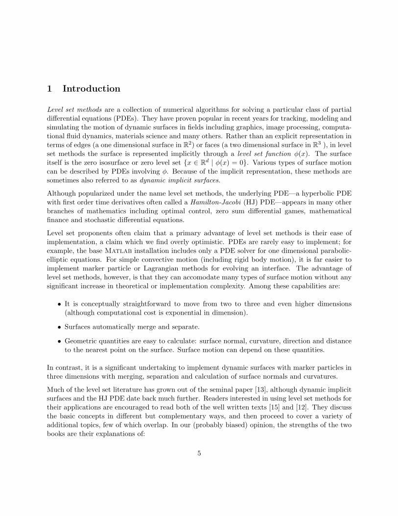
1 Introduction

Level set methods are a collection of numerical algorithms for solving a particular class of partialdifferential equations (PDEs). They have proven popular in recent years for tracking, modeling andsimulating the motion of dynamic surfaces in fields including graphics, image processing, computa-tional fluid dynamics, materials science and many others. Rather than an explicit representation interms of edges (a one dimensional surface in R2) or faces (a two dimensional surface in R3 ), in levelset methods the surface is represented implicitly through a level set function φ(x). The surfaceitself is the zero isosurface or zero level set {x ∈ Rd | φ(x) = 0}. Various types of surface motioncan be described by PDEs involving φ. Because of the implicit representation, these methods aresometimes also referred to as dynamic implicit surfaces.

Although popularized under the name level set methods, the underlying PDE—a hyperbolic PDEwith first order time derivatives often called a Hamilton-Jacobi (HJ) PDE—appears in many otherbranches of mathematics including optimal control, zero sum differential games, mathematicalfinance and stochastic differential equations.

Level set proponents often claim that a primary advantage of level set methods is their ease ofimplementation, a claim which we find overly optimistic. PDEs are rarely easy to implement; forexample, the base Matlab installation includes only a PDE solver for one dimensional parabolic-elliptic equations. For simple convective motion (including rigid body motion), it is far easier toimplement marker particle or Lagrangian methods for evolving an interface. The advantage oflevel set methods, however, is that they can accomodate many types of surface motion without anysignificant increase in theoretical or implementation complexity. Among these capabilities are:

• It is conceptually straightforward to move from two to three and even higher dimensions(although computational cost is exponential in dimension).

• Surfaces automatically merge and separate.

• Geometric quantities are easy to calculate: surface normal, curvature, direction and distanceto the nearest point on the surface. Surface motion can depend on these quantities.

In contrast, it is a significant undertaking to implement dynamic surfaces with marker particles inthree dimensions with merging, separation and calculation of surface normals and curvatures.

Much of the level set literature has grown out of the seminal paper [13], although dynamic implicitsurfaces and the HJ PDE date back much further. Readers interested in using level set methods fortheir applications are encouraged to read both of the well written texts [15] and [12]. They discussthe basic concepts in different but complementary ways, and then proceed to cover a variety ofadditional topics, few of which overlap. In our (probably biased) opinion, the strengths of the twobooks are their explanations of:

5

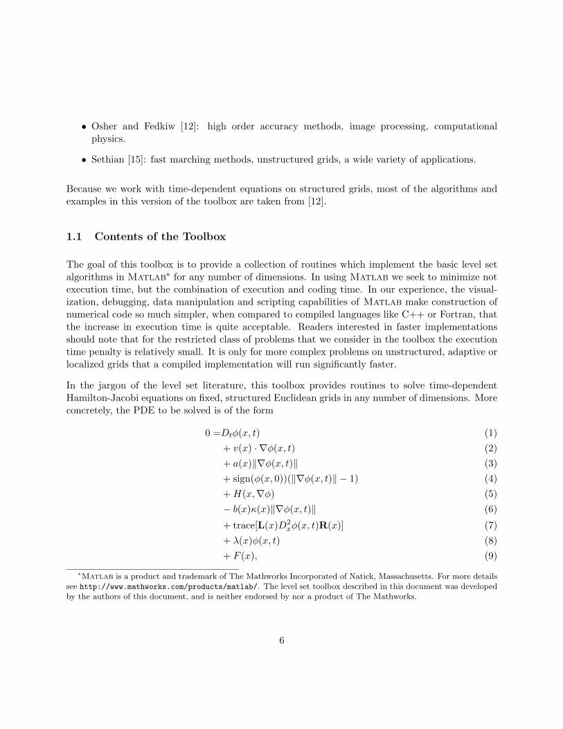
• Osher and Fedkiw [12]: high order accuracy methods, image processing, computationalphysics.

• Sethian [15]: fast marching methods, unstructured grids, a wide variety of applications.

Because we work with time-dependent equations on structured grids, most of the algorithms andexamples in this version of the toolbox are taken from [12].

1.1 Contents of the Toolbox

The goal of this toolbox is to provide a collection of routines which implement the basic level setalgorithms in Matlab∗ for any number of dimensions. In using Matlab we seek to minimize notexecution time, but the combination of execution and coding time. In our experience, the visual-ization, debugging, data manipulation and scripting capabilities of Matlab make construction ofnumerical code so much simpler, when compared to compiled languages like C++ or Fortran, thatthe increase in execution time is quite acceptable. Readers interested in faster implementationsshould note that for the restricted class of problems that we consider in the toolbox the executiontime penalty is relatively small. It is only for more complex problems on unstructured, adaptive orlocalized grids that a compiled implementation will run significantly faster.

In the jargon of the level set literature, this toolbox provides routines to solve time-dependentHamilton-Jacobi equations on fixed, structured Euclidean grids in any number of dimensions. Moreconcretely, the PDE to be solved is of the form

0 =Dtφ(x, t) (1)+ v(x) · ∇φ(x, t) (2)+ a(x)‖∇φ(x, t)‖ (3)+ sign(φ(x, 0))(‖∇φ(x, t)‖ − 1) (4)+H(x,∇φ) (5)− b(x)κ(x)‖∇φ(x, t)‖ (6)

+ trace[L(x)D2xφ(x, t)R(x)] (7)

+ λ(x)φ(x, t) (8)+ F (x), (9)

∗Matlab is a product and trademark of The Mathworks Incorporated of Natick, Massachusetts. For more detailssee http://www.mathworks.com/products/matlab/. The level set toolbox described in this document was developedby the authors of this document, and is neither endorsed by nor a product of The Mathworks.

6

subject to constraints

Dtφ(x, t) ≥ 0, Dtφ(x, t) ≤ 0, (10)φ(x, t) ≤ ψ(x), φ(x, t) ≥ ψ(x), (11)

where x ∈ Rn is the state space, φ : Rn × R → R is the level set function and ∇φ(x, t) =Dxφ(x, t) is the gradient of φ. Note that the time derivative (1) and at least one term involving aspatial derivative (2)–(7) must appear, otherwise the equation is not a hyperbolic PDE. Numericalapproximations for each type of term are provided.

• Time derivative (1) is approximated with an explicit total variation diminishing Runge-Kuttaintegration scheme with order of accuracy between one and three [12, chapter 3.5]. Becauseit is an explicit integrator, CFL conditions restrict the size of each timestep. An example isgiven in section 2.1 and a description of the toolbox routines in section 3.5.

• Motion by a constant velocity field (2), also called advection or convection. The user providesthe velocity field v : Rn → Rn, and the gradient ∇φ(x, t) is approximated with an upwindfinite difference scheme with order of accuracy between one and five [12, chapter 3]. Anexample is given in section 2.1, a description of the toolbox routines for upwind finite differenceapproximations in section 3.4.1, and a description of the toolbox routine for approximatingconstant velocity flow fields in section 3.6.1.

• Motion in the normal direction (3). The user provides the speed of the interface a : Rn → R,and ∇φ(x, t) is approximated with an upwind finite difference scheme [12, chapter 6]. Anexample is given in section 2.3.2 and a description of the toolbox routine in section 3.6.1.

• The reinitialization equation (4). This term is identically zero for signed distance functions,and can be applied to implicit surface functions in order to transform them into signed dis-tance functions [12, chapter 7.4]. A Godunov scheme for its solution can be found in [5,appendix A.3], which allows this term to be stably approximated with a minimum of artificialdissipation. Note that the initial conditions are used inside the signum function. An exampleis given in section 2.2.1 and a description of the toolbox routine in section 3.6.1. Reinitial-ization is usually applied as an auxiliary step by itself; a helper routine for this process isdescribed in section 3.7.3.

• A general Hamilton-Jacobi term (5) can treat a variety of applications, including optimalcontrol and differential games. The user provides the analytic Hamiltonian H : Rn×Rn → R.Upwind finite difference approximations of ∇φ(x, t) are provided, and Lax-Friedrichs is usedto stably approximate the H(x, p) function (with various options for the degree of localizationwhen calculating the artificial dissipation coefficient) [12, chapter 5]. An example is given insection 2.2.2 and a description of the toolbox routines in section 3.6.2.

7

• Motion by mean curvature (6). The user provides the speed b : Rn → R+, while the meancurvature κ(x) and gradient ∇φ(x, t) are approximated by centered second order accuratefinite difference approximations [12, chapter 4]. An example is given in section 2.3.1, a de-scription of the toolbox routines for centered finite difference approximations in section 3.4.2,and a description of the toolbox routine for motion by mean curvature in section 3.6.3.

• Motion by the trace of the Hessian (7), which arises from the Kolmogorov or Fokker-Plankequations when working with stochastic differential equations [6, 10]. The user providesthe matrices L,R : Rn → Rn×n, while the Hessian matrix of mixed second order spatialderivatives D2

xφ(x, t) is approximated by centered second order accurate finite difference ap-proximations. This feature has not yet been implemented, but will be available in futurereleases.

• Discounting terms (8), which arise when solving some types of optimal control problems [1]or stochastic differential equations [10] (in which context they relate to the “killing” process).The user provides the discount factor λ : Rn → R. This feature has not yet been implemented,but will be available in future releases.

• Forcing terms (9), which the user provides F : Rn → R. This feature has not yet beenimplemented, but will be available in future releases.

• Constraints (10) that the implicit surface should not grow or should not shrink. An exampleis given in section 2.2 and a description of the toolbox routine in section 3.6.4.

• Constraints (11) that the implicit surface should not enter or should not exit another implicitsurface. The user provides ψ : Rn → R defining the other implicit surface. Unlike most otherterms, this constraint is handled in an indirect manner using the postTimestep option of thetime integration routines. The option is discussed in section 3.5.3, and an example is givenin section 2.2.3.

This collection of terms covers most of the cases arising in applications, although the toolbox isorganized so that adding more types of terms is relatively straightforward.

1.2 Using the Toolbox

The best way to start is by looking at the examples, in particular the annotated example describedin section 2.1. Hopefully, most problems will be similar to one or more of the examples fromsection 2, so that one of those routines can be modified rather than starting from scratch.

When it comes time to develop code that implements a new application, there are several basicsteps that should be followed.

8

1. Determine the Hamilton-Jacobi equation.

2. Pick out the relevant types of terms from (1)–(11).

3. If upwinded approximations of first order derivatives are required, decide on the desired orderof accuracy.

4. Provide the other parameters needed by the HJ term approximations (velocities, speeds,matrices, discount factors, etc.).

5. Decide on the desired order of accuracy for the time derivative approximation, and the CFLnumber.

6. Pick the boundary conditions.

7. Create the grid.

8. Create the initial condition φ(x, 0).

9. Integrate forward in time, with occasional pauses to display or save the results.

1.3 Troubleshooting

Based on the author’s experience, common mistakes include:

• Too coarse a grid. Static implicit surface functions cannot resolve details of surface featuresthat are smaller than a grid cell. Dynamic evolution of those surfaces using the schemesdescribed here introduces numerical dissipation, so that even features whose size is a few gridcells may be smoothed away. In general, any important features must be at least three tofive grid cells wide in each dimension in order for them to be maintained for more than a fewtimesteps, even when using methods with high order accuracy. In some cases, a sufficientlyfine regular grid may be too computationally expensive to evolve and adaptive meshing maybe required.

• Poor dimensional scaling. Signed distance functions and the PDE solvers included in thistoolbox work best if all the dimensions in the problem are approximately the same size; forexample, the grid ranges and cell widths should be within an order of magnitude of oneanother. If dimensions involve widely different scales—such as radians and thousands offeet—then the problem parameters should be scaled to bring the dimensional ranges closertogether. Care must be taken in this process to ensure that all ranges, dynamics and otherparameters (such as bounds on partial derivative magnitudes) are scaled by the same amount.

9

• Incorrect initialization. If no implicit surface can be seen at t = 0, two quick checks should beperformed. First, make sure that the desired implicit surface falls within the bounds of thecomputational grid (as defined by the structure members grid.min and grid.max). Second,make sure that the desired implicit surface is at least two grid cells wide in each dimension(the width of a grid cell is given by the structure member grid.dx).

• Numerical instability. The level set function may become highly oscillatory, a behavior whichmanifests itself by the sudden appearance of many convoluted looking surfaces in two di-mensional contour or three dimensional isosurface plots. Instability can be caused by buggyboundary conditions, poor dimensional scaling, incorrect CFL restrictions (for example, if thebounds on the partial derivative of the Hamiltonian are too small when solving a problemwith a general HJ term (5)), or bugs in the kernel.

• Sign problems. If the surface seems to be moving in the wrong direction, try switching thesign of the flow.

1.4 Advanced Tips for the Toolbox

We heartily endorse attempts to modify the toolbox, add to it, or use some of its more advancedfeatures (such as general Hamilton-Jacobi terms); however, we do have some recommendations.

• Start with a simplified example that is known to work, and add features incrementally withtests until the full version is achieved.

• Start with low order accurate approximations on a reasonably coarse grid. If it works, improvethe accuracy. Often it is more efficient to increase the order of accuracy of the approximationsthan to refine the grid.

• Learn how to use Matlab’s debugging and visualization systems. One of the reasons thatstructures were used extensively in this version (rather than full blown classes) was to allowtheir contents to be examined easily during debugging at any level of the stack. Further-more, the ability to produce contour and isosurface plots at the debugger command linemakes debugging of two and three dimensional code merely unpleasant, instead of virtuallyimpossible.

• Learn Matlab’s cell arrays (arrays written with “{}” instead of “()”). In order to createdimensionally independent code, cell arrays were used extensively in the kernel code. Inparticular, if data is an n dimensional (regular) array and indices is a cell vector of length n(a two dimensional cell array of size n×1) each element of which is a regular vector, then thesyntax data(indices{:}) can be used to pick out subsets and slices of data. For example,

10

if data = rand([10 10 10]) and indices = { 2:9; 4:6; 5 }, then data(indices{:}) =data(2:9,4:6,5). More generally, the notation indices{:} turns the elements of the cellarray indices into a comma separated list that can be used either to index into an array or asthe parameter list for a function; for example, to call interpn in a dimensionally independentway. Another very useful function for cell arrays is Matlab’s deal; for example, the help textof deal shows how to collect the comma separated list of parameters returned by a functioninto a single cell array.

• Learn how to vectorize in the Matlab sense. Despite working in Matlab’s interpretedprogramming environment, this toolbox can achieve nearly the performance of compiled code.In order to achieve this performance, it is important never to loop explicitly over the elementsof the data array. Instead, all operations on the data array are written as element-wise sums,products (“.*”) and logical comparisons. The result is not as memory efficient as could beachieved in a carefully constructed compiled code, but it is far better than explicit loops.

• Tell us if you find a repeatable bug.

11

2 Level Set Examples

Our examples fall into three categories: those that are motivated by specific examples taken frompapers or texts, those that demonstrate the basic capabilities of the toolbox, and those designed totest aspects of the implementation. The code implementing most of the examples in the former twocategories follows a similar structures, so as a starting point, we provide an extensively annotatedscript file which shows how to implement motion by an external velocity field.

The first step to running the examples described in this section is to modify the script file Examples/addPathToKernelso that it contains the absolute path name for the Kernel directory. The absolute path name isrequired because current versions of Matlab appear unable to create function handles involvingrelative path names. Once this modification is performed, it should be possible to enter into anyof the example subdirectories, start Matlab, and execute one of the examples by typing its nameat the Matlab prompt.

2.1 Getting Started: Convective Motion (2)

In this section we examine in detail how to implement motion by an external velocity field (2) usingthe file Examples/Basic/convectionDemo. The implementation of many of the other examplesfollows the same basic framework.

[ data, g, data0 ] = convectionDemo(flowType, accuracy, displayType): Demonstratemotion by an external velocity field. The three input parameters are strings; the optionsfor the first two are explained in the help text and the options for displayType come directlyfrom the helper routine visualizeLevelSet. All three input parameters are optional. Thereturned parameters are the final φ(x, tmax) function data, the computational grid g and theinitial φ(x, 0) function data0.

Figure 1 shows the results of running convectionDemo(’linear’, ’medium’). Beyond the threeinput parameters, there are many other options to the way this example runs and is displayed.These options can be easily modified by editing the source of convectionDemo directly.

• Initial and final time.

• Whether to display intermediate results. If so, how many intermediate results, whetherto display results in a single figure or as a sequence of subplots, whether to pause betweenvisualizations, and whether to remove visualizations from previous timesteps before displayingthe next.

12

Figure 1: Result of running convectionDemo(’linear’, ’medium’). Shows motion by a constantrotational external velocity field.

• Grid parameters: dimension, resolution, periodic or extrapolating boundary conditions.

• Details of the velocity field.

• Shape and location of the initial surface.

For more details, see the commentary below. Increasing accuracy will increase execution time.Table 1 shows the execution times for each of the accuracy options with flowType = ’linear’.In order to get better resolution of the execution time, the grid resolution was doubled to g.dx= 0.01 (see below for details on how to make this change). The computational platform was aPentium 4 with plenty of memory running Matlab 6.5 in Windows XP Professional. Examiningthe figures, the low accuracy run had clearly lost area by the end of the full rotation (at tmax)but the remaining choices were visually indistinguishable. A quantitative error comparison will beperformed when somebody has the time to write the scripts.

We now examine the components of the source code for convectionDemo. Notice that most of thefile is concerned with initialization, since the toolbox and Matlab handle the real work.

13

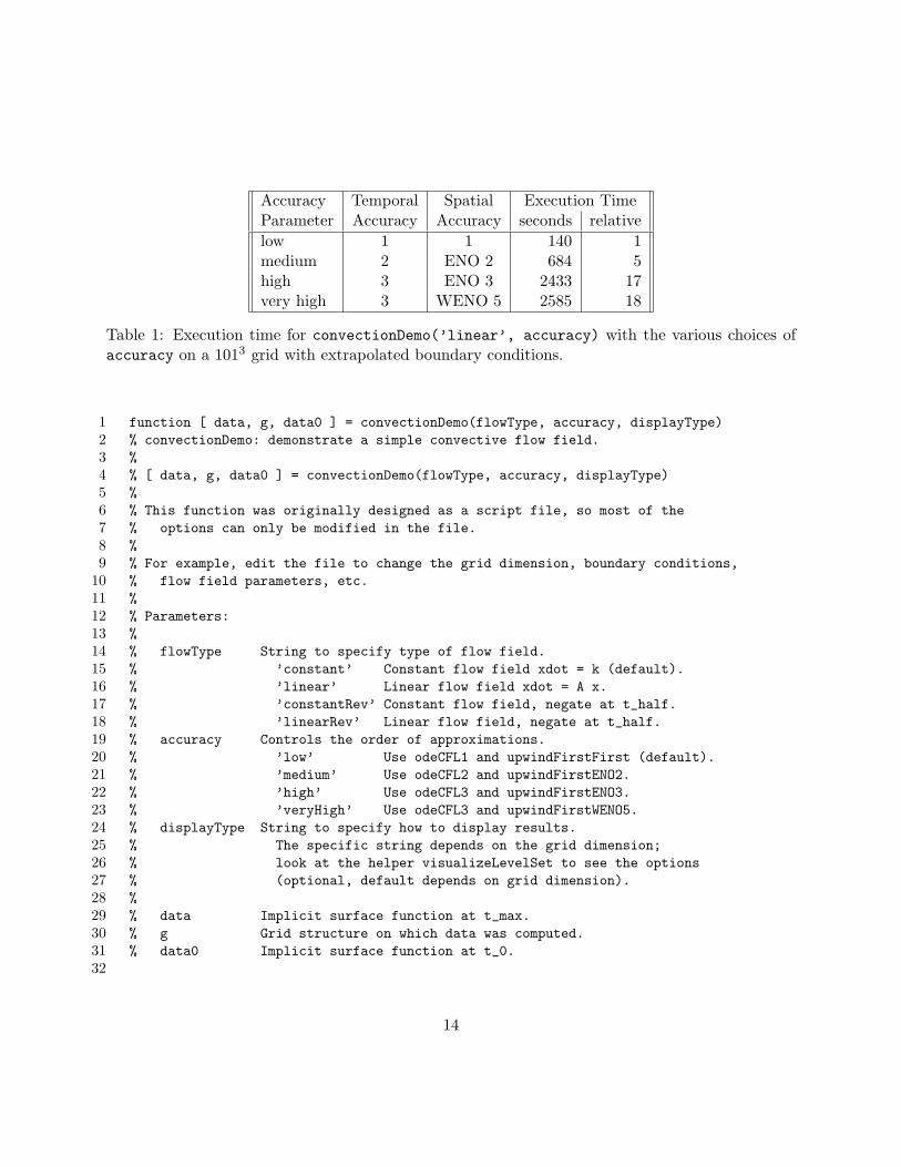
Accuracy Temporal Spatial Execution TimeParameter Accuracy Accuracy seconds relativelow 1 1 140 1medium 2 ENO 2 684 5high 3 ENO 3 2433 17very high 3 WENO 5 2585 18

Table 1: Execution time for convectionDemo(’linear’, accuracy) with the various choices ofaccuracy on a 1013 grid with extrapolated boundary conditions.

1 function [ data, g, data0 ] = convectionDemo(flowType, accuracy, displayType)2 % convectionDemo: demonstrate a simple convective flow field.3 %4 % [ data, g, data0 ] = convectionDemo(flowType, accuracy, displayType)5 %6 % This function was originally designed as a script file, so most of the7 % options can only be modified in the file.8 %9 % For example, edit the file to change the grid dimension, boundary conditions,

10 % flow field parameters, etc.11 %12 % Parameters:13 %14 % flowType String to specify type of flow field.15 % ’constant’ Constant flow field xdot = k (default).16 % ’linear’ Linear flow field xdot = A x.17 % ’constantRev’ Constant flow field, negate at t_half.18 % ’linearRev’ Linear flow field, negate at t_half.19 % accuracy Controls the order of approximations.20 % ’low’ Use odeCFL1 and upwindFirstFirst (default).21 % ’medium’ Use odeCFL2 and upwindFirstENO2.22 % ’high’ Use odeCFL3 and upwindFirstENO3.23 % ’veryHigh’ Use odeCFL3 and upwindFirstWENO5.24 % displayType String to specify how to display results.25 % The specific string depends on the grid dimension;26 % look at the helper visualizeLevelSet to see the options27 % (optional, default depends on grid dimension).28 %29 % data Implicit surface function at t_max.30 % g Grid structure on which data was computed.31 % data0 Implicit surface function at t_0.32

14

33 % Ian Mitchell, 2/9/043435 %---------------------------------------------------------------------------36 % You will see many executable lines that are commented out.37 % These are included to show some of the options available; modify38 % the commenting to modify the behavior.39

Standard opening comments, including the help text. The blank line 32 ensures that subsequentcomment lines are not included in the help entry. Notice the options for input parameters flowTypeand accuracy.

40 %---------------------------------------------------------------------------41 % Make sure we can see the kernel m-files.42 run(’../addPathToKernel’);43

To make sense of the function calls and function handles encountered in the remainder of the file,the kernel directories must be on Matlab’s path. The script Examples/addPathToKernel addsthe Kernel directory and all its subdirectories to Matlab’s path if they are not already present(so repeated executions of addPathToKernel are safe). We use the functional form of run in orderto access the parent directory.

44 %---------------------------------------------------------------------------45 % Integration parameters.46 tMax = 1.0; % End time.47 plotSteps = 9; % How many intermediate plots to produce?48 t0 = 0; % Start time.49 singleStep = 0; % Plot at each timestep (overrides tPlot).5051 % Period at which intermediate plots should be produced.52 tPlot = (tMax - t0) / (plotSteps - 1);5354 % How close (relative) do we need to get to tMax to be considered finished?55 small = 100 * eps;5657 %---------------------------------------------------------------------------58 % What level set should we view?59 level = 0;6061 % Pause after each plot?

15

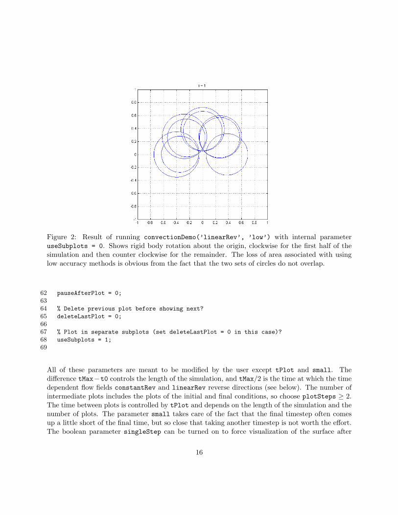
Figure 2: Result of running convectionDemo(’linearRev’, ’low’) with internal parameteruseSubplots = 0. Shows rigid body rotation about the origin, clockwise for the first half of thesimulation and then counter clockwise for the remainder. The loss of area associated with usinglow accuracy methods is obvious from the fact that the two sets of circles do not overlap.

62 pauseAfterPlot = 0;6364 % Delete previous plot before showing next?65 deleteLastPlot = 0;6667 % Plot in separate subplots (set deleteLastPlot = 0 in this case)?68 useSubplots = 1;69

All of these parameters are meant to be modified by the user except tPlot and small. Thedifference tMax−t0 controls the length of the simulation, and tMax/2 is the time at which the timedependent flow fields constantRev and linearRev reverse directions (see below). The number ofintermediate plots includes the plots of the initial and final conditions, so choose plotSteps ≥ 2.The time between plots is controlled by tPlot and depends on the length of the simulation and thenumber of plots. The parameter small takes care of the fact that the final timestep often comesup a little short of the final time, but so close that taking another timestep is not worth the effort.The boolean parameter singleStep can be turned on to force visualization of the surface after

16

every CFL constrained timestep. It is mostly useful for debugging, and we recommend choosingdeleteLastPlot = 1 and useSubplots = 0 if you choose singleStep = 1. If useSubplots = 0,then all visualizations are done in a single full figure axis. Figure 2 shows the results of runningconvectionDemo(’linearRev’,’low’) when the source is modified to set the internal parameteruseSubplots = 0. The parameter level chooses which isosurface of φ is visualized when usingcontour plots (in 2D) or surfaces (in 3D).

70 %---------------------------------------------------------------------------71 % Use periodic boundary conditions?72 periodic = 0;7374 % Create the grid.75 g.dim = 2;76 g.min = -1;77 g.dx = 1 / 50;78 if(periodic)79 g.max = (1 - g.dx);80 g.bdry = @addGhostPeriodic;81 else82 g.max = +1;83 g.bdry = @addGhostExtrapolate;84 end85 g = processGrid(g);86

This block of code creates the computational grid. The user may modify the boolean flag periodicto choose whether periodic or extrapolation boundary conditions are used (or choose something elseby setting g.bdry). Dimension is set with g.dim and resolution with g.dx. Since all dimensionshave the same resolution, bounds and boundary conditions, it is only necessary to store scalarsand single function handles in the fields. The call to processGrid automatically extends all fields(except g.dim) to their full vector length. Missing fields are given inferred values (such as g.N) ordefaults (such as g.bdryData). Figure 3 shows the results of running this example in dimensionsone and three.

87 %---------------------------------------------------------------------------88 % Most of the time in constant flow case, we want flow in a89 % distinguished direction, so assign first dimension’s flow separately.90 constantV = 0 * ones(g.dim);91 constantV(1) = 2;92 constantV = num2cell(constantV);93

17

(a) (b)

Figure 3: Running convectionDemo in other dimensions by modifying the internal parameterg.dim. These are not exactly the figures generated during the run: the subplots generated dur-ing the run have had their axis bounds adjusted to be consistent across all nine subplots ineach case. Figure 3(a): The implicit surface function φ for a one dimensional example run byconvectionDemo(’constantRev’, ’veryHigh’). Figure 3(b): An isosurface plot for a three di-mensional example run by convectionDemo(’linear’, ’medium’).

94 % Create linear flow field xdot = A * x95 linearA = 2 * pi * [ 0 1 0 0; -1 0 0 0; 0 0 0 0; 0 0 0 0 ];96 %linearA = eye(4);97 indices = { 1:g.dim; 1:g.dim };98 linearV = cellMatrixMultiply(num2cell(linearA(indices{:})), g.xs);99

Flow fields are defined by cell vectors. Element i of the cell vector gives the motion in the ith

dimensions. Element i can be either a scalar—if the flow field does not depend on x—or an arrayof size grid.shape, each element of which gives the motion in dimension i for the correspondingnode of the grid. While Matlab has many ways to generate regular vectors, matrices and arrays,there are few ways to similarly populate cell arrays. This block of code demonstrates a few, includingthe very useful num2cell.

The constant flow field v(x) = constantV demonstrates a spatially independent flow field, in thiscase a flow field with speed two along the first dimension. The linear flow field v(x) = Ax = linearVdemonstrates the spatially dependent flow field. In order to allow for variable dimension, the

18

array A = linearA is defined up to dimension 4. Line 95 provides a definition of A whichgenerates rotation about the origin in the x1-x2 plane. Line 96 can be uncommented to generatean exponentially growing surface. The magic is performed in line 98, where cellMatrixMultiplycomputes Ax at every node x in the grid. In particular, the appropriate g.dim × g.dim subset oflinearA is picked out by indices{:}, which turns the indices cell vector into a comma separatedlist that can be used as an argument to a function or (in this case) an index into an array. This“{:}” construction is used extensively throughout the toolbox to provide dimensionally independentcode.

100 %---------------------------------------------------------------------------101 if(nargin < 1)102 flowType = ’constant’;103 end104105 % Choose the flow field.106 switch(flowType)107108 case ’constant’109 v = constantV;110111 case ’linear’112 v = linearV;113114 case ’constantRev’115 v = @switchValue;116 schemeData.one = constantV;117 schemeData.two = cellMatrixMultiply(-1, constantV)118 schemeData.tSwitch = 0.5 * tMax;119120 case ’linearRev’121 v = @switchValue;122 schemeData.one = linearV;123 schemeData.two = cellMatrixMultiply(-1, linearV)124 schemeData.tSwitch = 0.5 * tMax;125126 otherwise127 error(’Unknown flowType %s’, flowType);128129 end130

This block of code picks out which velocity field will be used in the run. The default flow field isdetermined by line 102. The first two cases of flow field ’constant’ and ’linear’ are straight-forward, and show how to create a time independent flow field using a constant cell vector. For

19

time dependent flow fields, a function handle is passed instead. The function switchValue is de-scribed below. It requires that the schemeData structure have some additional fields beyond thoserequired by termConvection: one, two, and tSwitch (these additional fields will be ignored bytermConvection). Note the use of cellMatrixMultiply with a scalar parameter to reverse thedirection of the flow fields for the second half of the simulation.

131 %---------------------------------------------------------------------------132 % What kind of display?133 if(nargin < 3)134 switch(g.dim)135 case 1136 displayType = ’plot’;137 case 2138 displayType = ’contour’;139 case 3140 displayType = ’surface’;141 otherwise142 error(’Default display type undefined for dimension %d’, g.dim);143 end144 end

The default visualization style for each of dimensions 1–3 is set by this block of code. While thetoolbox is almost entirely dimensionally independent, and the version of convectionDemo describedhere will work computationally for dimensions up to four, visualization is challenging for dimensionsgreater than three.

145 %---------------------------------------------------------------------------146 % Create initial conditions (a circle/sphere).147 % Note that in the periodic BC case, these initial conditions will not148 % be continuous across the boundary unless the circle is perfectly centered.149 % In practice, we’ll just ignore that little detail.150 center = [ -0.4; 0.0; 0.0; 0.0 ];151 radius = 0.35;152 data = zeros(size(g.xs{1}));153 for i = 1 : g.dim154 data = data + (g.xs{i} - center(i)).^2;155 end156 data = sqrt(data) - radius;157 data0 = data;158

20

The initial conditions are a sphere in dimension grid.dim of radius radius centered at center.Note the vectorized use of g.xs to determine the initial implicit surface function (in fact, this is asigned distance function).

159160 %---------------------------------------------------------------------------161 if(nargin < 2)162 accuracy = ’low’;163 end164165 % Set up spatial approximation scheme.166 schemeFunc = @termConvection;167 schemeData.velocity = v;168 schemeData.grid = g;169170 % Set up time approximation scheme.171 integratorOptions = odeCFLset(’factorCFL’, 0.5, ’stats’, ’on’);172173 % Choose approximations at appropriate level of accuracy.174 switch(accuracy)175 case ’low’176 schemeData.derivFunc = @upwindFirstFirst;177 integratorFunc = @odeCFL1;178 case ’medium’179 schemeData.derivFunc = @upwindFirstENO2;180 integratorFunc = @odeCFL2;181 case ’high’182 schemeData.derivFunc = @upwindFirstENO3;183 integratorFunc = @odeCFL3;184 case ’veryHigh’185 schemeData.derivFunc = @upwindFirstWENO5;186 integratorFunc = @odeCFL3;187 otherwise188 error(’Unknown accuracy level %s’, accuracy);189 end190191 if(singleStep)192 integratorOptions = odeCFLset(integratorOptions, ’singleStep’, ’on’);193 end194

This block sets up function handles for both the spatial approximation scheme schemeFunc and thetime integration scheme integratorFunc. The default accuracy is determined by line 162. The

21

meaning of each level of accuracy is determined by the switch/case statement. The flow fieldinformation which was determined earlier is stored into schemeData.velocity. In line 192, noticethat an existing odeCFLn option structure is modified if single stepping has been requested.

195 %---------------------------------------------------------------------------196 % Initialize Display197 f = figure;198199 % Set up subplot parameters if necessary.200 if(useSubplots)201 rows = ceil(sqrt(plotSteps));202 cols = ceil(plotSteps / rows);203 plotNum = 1;204 subplot(rows, cols, plotNum);205 end206207 h = visualizeLevelSet(g, data, displayType, level, [ ’t = ’ num2str(t0) ]);208209 hold on;210 if(g.dim > 1)211 axis(g.axis);212 daspect([ 1 1 1 ]);213 end214

This block of code performs basic display initialization. If subplots have been requested, the layoutof the subplot array must be determined. Before calling visualizeLevelSet to perform the actualvisualization, we make current the appropriate figure axis with either figure or subplot. The cur-rent time is passed in a string for use as the title of the figure. As a side effect, visualizeLevelSetwill finish with a call to drawnow to ensure that the results are shown before computation proceeds.Because this call to drawnow is performed before the modifications in lines 211–212, they may notbe immediately visible.

215 %---------------------------------------------------------------------------216 % Loop until tMax (subject to a little roundoff).217 tNow = t0;218 startTime = cputime;219 while(tMax - tNow > small * tMax)220221 % Reshape data array into column vector for ode solver call.222 y0 = data(:);223

22

224 % How far to step?225 tSpan = [ tNow, min(tMax, tNow + tPlot) ];226227 % Take a timestep.228 [ t y ] = feval(integratorFunc, schemeFunc, tSpan, y0,...229 integratorOptions, schemeData);230 tNow = t(end);231232 % Get back the correctly shaped data array233 data = reshape(y, g.shape);234

This is the heart of the simulation, where all of the work is accomplished. Integration of theunderlying PDE is accomplished entirely by lines 228–229. Lines 222 and 233 massage the arraydata that stores the implicit surface function φ into the shape required by the integrator functionsintegratorFunc = @odeCFLn and back again. Lines 219, 225 and 230 keep track of the passage ofsimulation time.

235 if(pauseAfterPlot)236 % Wait for last plot to be digested.237 pause;238 end239240 % Get correct figure, and remember its current view.241 figure(f);242 figureView = view;243244 % Delete last visualization if necessary.245 if(deleteLastPlot)246 delete(h);247 end248249 % Move to next subplot if necessary.250 if(useSubplots)251 plotNum = plotNum + 1;252 subplot(rows, cols, plotNum);253 end254255 % Create new visualization.256 h = visualizeLevelSet(g, data, displayType, level, [ ’t = ’ num2str(tNow) ]);257258 % Restore view.259 view(figureView);

23

260261 end262263 endTime = cputime;264 fprintf(’Total execution time %g seconds’, endTime - startTime);265266267

These remaining lines complete the while loop that manages simulation time and the convectionDemofunction as a whole. They are devoted to visualization.

268 %---------------------------------------------------------------------------269 %%%%%%%%%%%%%%%%%%%%%%%%%%%%%%%%%%%%%%%%%%%%%%%%%%%%%%%%%%%%%%%%%%%%%%%%%%%%270 %---------------------------------------------------------------------------271 function out = switchValue(t, data, schemeData)272 % switchValue: switches between two values.273 %274 % out = switchValue(t, data, schemeData)275 %276 % Returns a constant value:277 % one for t <= tSwitch;278 % two for t > tSwitch.279 %280 % By setting one and two correctly, this function can implement281 % the velocityFunc prototype for termConvection;282 % the scalarGridFunc prototype for termNormal, termCurvature and others;283 % and possibly some other prototypes...284 %285 % Parameters:286 % t Current time.287 % data Level set function.288 % schemeData Structure (see below).289 %290 % out Either schemeData.one or schemeData.two.291 %292 % schemeData is a structure containing data specific to this type of293 % term approximation. For this function it contains the field(s)294 %295 % .one The value to return for t <= tSwitch.296 % .two The value to return for t > tSwitch.297 % .tSwitch The time at which the switch between flow fields occurs.298 %

24

299 % schemeData may contain other fields.300301 checkStructureFields(schemeData, ’one’, ’two’, ’tSwitch’);302303 if(t <= schemeData.tSwitch)304 out = schemeData.one;305 else306 out = schemeData.two;307 end308

This subfunction switchValue within convectionDemo is an example of a function satisfying thevelocityFunc prototype for the term approximation termConvection (see section 3.6.1). It imple-ments a time dependent flow field by choosing one of two constant flow fields based on the currenttime. This simple time dependent function also satisfies the scalarGridFunc prototype (assumingthat schemeData.one and schemeData.two are set appropriately), and is used in the examplesnormalStarDemo and curvatureStarDemo in section 2.3. Much more complex time dependentvelocity fields are possible with this framework.

2.2 Basic Examples

This section discusses functions found in the directory Examples/Basic. This directory providesan example for each of the types of spatial terms (4)–(11) with the exception of motion by meancurvature (6). Examples for the omitted terms can be found elsewhere: section 2.1 for motion bya constant velocity field (2) and section 2.3 for motion in the normal direction (3) and motion bymean curvature (6). Since terms (8)–(11) do not include a spatial derivative, examples for theseterms naturally include a combination with other types of term.

2.2.1 The Reinitialization Equation (4)

This section describes the function Examples/Basic/reinitDemo.

Reinitialization is the process of modifying an implicit surface function into a signed distancefunction—modifying φ such that ‖∇φ‖ ≈ 1 without moving its zero isosurface. One method ofreinitialization is to solve the reinitialization equation, which is a general HJ PDE with spatialterm (4). Under normal circumstances this task is accomplished with an auxiliary integrationroutine that hides the details; for example, see signedDistanceIterative in section 3.7.3 andreinitTest in section 2.7.3. However, for the purposes of demonstrating and testing the termapproximation function termReinit, we provide the following routine.

25

(a) φ(x, 0) (b) φ(x, tmax)

Figure 4: Comparing initial and final implicit surface functions for reinitDemo(’star’,’medium’, ’surf’). Notice how the slope of the final φ is much more consistent.

[ data, g, data0 ] = reinitDemo(initialType, accuracy, displayType): Demonstrate thereinitialization equation. The three input parameters are strings; the last two are the sameas for convectionDemo. The initialType can be either ’circle’ (an off center circle) or’star’ (a centered seven pointed star). All three input parameters are optional. The re-turned parameters are the final φ(x, tmax) function data, the computational grid g and theinitial φ(x, 0) function data0.

The internals of reinitDemo are virtually identical to convectionDemo, so we discuss them nofurther here.

In the ’circle’ case, the initial implicit surface function for an off center circle is not a signeddistance function because of the periodic boundary conditions. In the ’star’ case, the initialimplicit surface function does not have unit magnitude gradient (see (13) in section 2.3 for the initialimplicit surface equation). Figure 4 shows the results for the ’star’ case, while figure 5 shows howthe reinitialization procedure successfully adjusts the gradient magnitude without distorting thezero isosurface too badly. These results were calculated on a relatively coarse grid (g.dx = 0.02)using accuracy = ’medium’.

26

(a) {x | φ(x, t) = 0} (b) ‖∇φ(x, t)‖

Figure 5: Examining the effect of reinitialization on the implicit surface (the zero isosurface ofφ(x, t)) and the gradient magnitude. The implicit surface has moved only slightly, and at mostnodes φ(x, tmax) has close to unit magnitude gradient despite the large gradient of φ(x, 0). Usinga higher accuracy scheme would lead to even less movement of the implicit surface.

2.2.2 General HJ Terms (5)

This section describes the function Examples/Basic/laxFriedrichsDemo.

General Hamilton-Jacobi equations are challenging but useful in a wide variety of applications.In this section we look at how convective motion can be formulated as a general HJ, which isperhaps the simplest example of such equations. Since the methods for general HJ generally requirethe addition of artificial dissipation, this formulation is not usually appropriate for convectiveflow; instead, the specialized upwinded convection schemes should be used (see the example insection 2.1). More ambitious examples of general HJ can be found in sections 2.5 and 2.6.

[ data, g, data0 ] = laxFriedrichsDemo(flowType, initShape, accuracy, dissType, displayType):Demonstratean implementation of time independent convective flow using a general HJ solver. Thefour input parameters are strings. The parameters accuracy and displayType have thesame options as the identically named parameters of convectionDemo. The parameterflowType allows the time-independent flow fields permitted by convectionDemo. The param-eter initShape specifies the shape of the initial implicit surface. The parameter dissType

27

specifies which of the types of artificial dissipation functions to use to stabilize the Lax-Friedrichs solver. All five input parameters are optional. The returned parameters are thefinal φ(x, tmax) function data, the computational grid g and the initial φ(x, 0) function data0.

The internals of laxFriedrichsDemo are the same as convectionDemo, with the exception thatfunctions for the prototypes hamFunc and partialFunc must be provided. In addition, it demon-strates the use of termLaxFriedrichs and the routines implementing the dissFunc prototype:artificialDissipationGLF, artificialDissipationLLF, and artificialDissipationLLLF.

Formulating convection by flow field v(x) as a general HJ leads to Hamiltonian

H(x, p) = v(x) · p

This simple dot product is calculated by the subfunction laxFriedrichsDemoHamFunc (found inthe file laxFriedrichsDemo), which implements the hamFunc prototype. To scale the dissipation,we need

αi(x) = maxp

∣∣∣∣∂H(x, p)∂pi

∣∣∣∣ = |vi(x)|. (12)

This optimization over partials is performed by the subfunction laxFriedrichsDemoPartialFunc,which implements the partialFunc prototype. Note that the partials of H with respect to p areindependent of p; consequently the range of p in the maximization is irrelevant and the differenttypes of dissipation function (chosen by the parameter dissType of laxFriedrichsDemo) will allproduce the same results.

Do not be fooled by the simplicity of these hamFunc and partialFunc examples. Usually theyare much more difficult to compute. In most interesting cases the partial derivative of H withrespect to p will depend on p (otherwise the Hamiltonian represents a convective flow field), so themaximization in (12) will be nontrivial. Fortunately, it can be overapproximated if the optimizationis too challenging, at the cost of additional dissipation. For more details, see section 3.6.2.

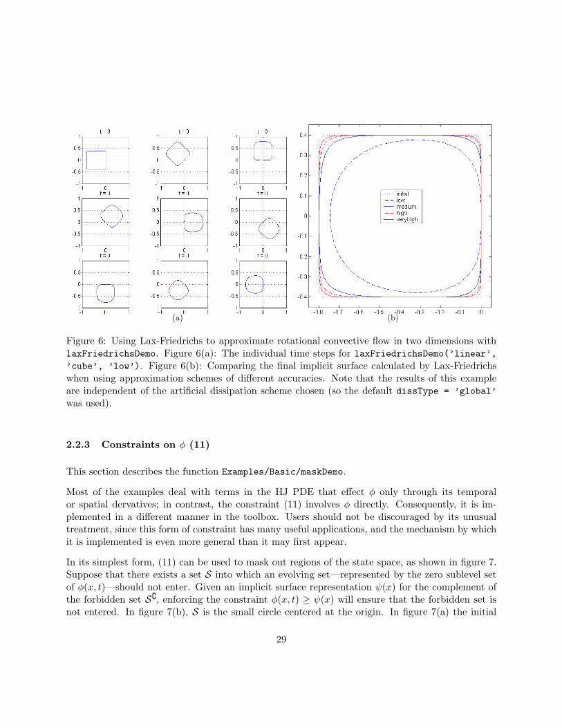
Figure 6 shows the results of running this example in two dimensions for a rigid body rotation ofa square. The dissipation which smooths away the corners of the square has two sources: errors inthe calculation of the first derivative and the Lax-Friedrichs’ artificial dissipation term. By usingan approximation scheme of higher order accuracy, the former can be reduced. The approximateexecution time (relative to accuracy = ’low’) for the four schemes were: ’low’ = 1, ’medium’= 4, ’high’ = 12 and ’veryHigh’ = 17.

28

(a) (b)

Figure 6: Using Lax-Friedrichs to approximate rotational convective flow in two dimensions withlaxFriedrichsDemo. Figure 6(a): The individual time steps for laxFriedrichsDemo(’linear’,’cube’, ’low’). Figure 6(b): Comparing the final implicit surface calculated by Lax-Friedrichswhen using approximation schemes of different accuracies. Note that the results of this exampleare independent of the artificial dissipation scheme chosen (so the default dissType = ’global’was used).

2.2.3 Constraints on φ (11)

This section describes the function Examples/Basic/maskDemo.

Most of the examples deal with terms in the HJ PDE that effect φ only through its temporalor spatial dervatives; in contrast, the constraint (11) involves φ directly. Consequently, it is im-plemented in a different manner in the toolbox. Users should not be discouraged by its unusualtreatment, since this form of constraint has many useful applications, and the mechanism by whichit is implemented is even more general than it may first appear.

In its simplest form, (11) can be used to mask out regions of the state space, as shown in figure 7.Suppose that there exists a set S into which an evolving set—represented by the zero sublevel setof φ(x, t)—should not enter. Given an implicit surface representation ψ(x) for the complement ofthe forbidden set S{, enforcing the constraint φ(x, t) ≥ ψ(x) will ensure that the forbidden set isnot entered. In figure 7(b), S is the small circle centered at the origin. In figure 7(a) the initial

29

(a) (b)

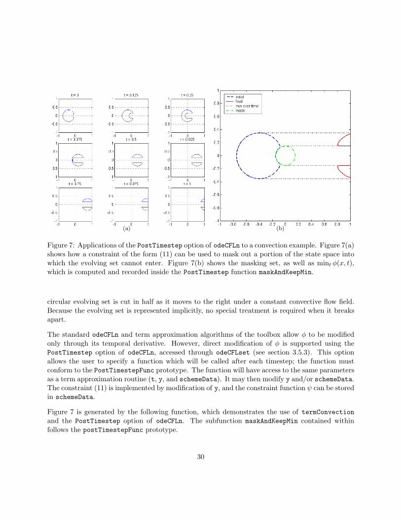
Figure 7: Applications of the PostTimestep option of odeCFLn to a convection example. Figure 7(a)shows how a constraint of the form (11) can be used to mask out a portion of the state space intowhich the evolving set cannot enter. Figure 7(b) shows the masking set, as well as mint φ(x, t),which is computed and recorded inside the PostTimestep function maskAndKeepMin.

circular evolving set is cut in half as it moves to the right under a constant convective flow field.Because the evolving set is represented implicitly, no special treatment is required when it breaksapart.

The standard odeCFLn and term approximation algorithms of the toolbox allow φ to be modifiedonly through its temporal derivative. However, direct modification of φ is supported using thePostTimestep option of odeCFLn, accessed through odeCFLset (see section 3.5.3). This optionallows the user to specify a function which will be called after each timestep; the function mustconform to the PostTimestepFunc prototype. The function will have access to the same parametersas a term approximation routine (t, y, and schemeData). It may then modify y and/or schemeData.The constraint (11) is implemented by modification of y, and the constraint function ψ can be storedin schemeData.

Figure 7 is generated by the following function, which demonstrates the use of termConvectionand the PostTimestep option of odeCFLn. The subfunction maskAndKeepMin contained withinfollows the postTimestepFunc prototype.

30

[ data, g, data0 ] = maskDemo(accuracy, displayType): Demonstrates applications of thePostTimestep option of odeCFLn, using a simple convective flow field. The parametersaccuracy and displayType are as normal. Plotting routines at the end of the functionare specialized to two dimensional grids, and demonstrate the effects of the PostTimestepcalls. The figure 7(b) is generated by these plotting routines.

The PostTimestep mechanism is more general than just constraints of the form (11). Changes tothe term approximation parameters in schemeData can effect the evolution of the interface; however,there are often ways to achieve the same effect directly in the term approximation routine. A betteruse is to record information about the changes to φ during the integration. This application isdemonstrated in maskDemo as well, where the field schemeData.min is used to record mint φ(x, t)as the integration proceeds.

Users should note that modification of schemeData can carry a signficant performance penalty, sinceall of its large fields (such as schemeData.grid) will be copied at each timestep. Consequently,this modification mechanism should be used only when no other mechanism can achieve the sameresult.

2.3 Examples from Osher & Fedkiw [12]

This section describes functions in the directory Examples/OsherFedkiw/.

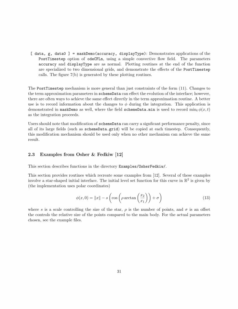
This section provides routines which recreate some examples from [12]. Several of these examplesinvolve a star-shaped initial interface. The initial level set function for this curve in R2 is given by(the implementation uses polar coordinates)

φ(x, 0) = ‖x‖ − s

(cos(ρ arctan

(x2

x1

))+ σ

)(13)

where s is a scale controlling the size of the star, ρ is the number of points, and σ is an offsetthe controls the relative size of the points compared to the main body. For the actual parameterschosen, see the example files.

31

Figure 8: Motion by mean curvature (compare with [12, figure 4.1]). The initial implicit surfacefunction is generated from an ellipse in polar coordinates, rather than the original point clouddescription of the problem [13, 12].

2.3.1 Motion by Mean Curvature (6)

This section describes the functions curvatureSpiralDemo, curvatureStarDemo, spiralFromEllipseand spiralFromPoints in the directory Examples/OsherFedkiw/.

The first example of motion by mean curvature is a classic taken from [13] and shown in figure 8:motion of a two dimensional wound spiral interface. This example and the next demonstrate theuse of termCurvature.

[ data, g, data0 ] = curvatureSpiralDemo(accuracy, initial, displayType): Demonstratesmotion by mean curvature on a two dimensional wound spiral interface. The accuracy anddisplayType parameters are as normal. The string parameter initial chooses how to con-struct the initial implicit surface function. The options are ’ellipse’ (the default) and’points’. These initial conditions are specifically designed for two dimensional grids.

32

(a) (b)

Figure 9: Motion by mean curvature. Figure 9(a) shows motion with constant multiplier b, theresult of curvatureStarDemo with default parameters (compare with [12, figure 4.2]). Figure 9(b)uses a time and spatially varying multiplier b(x, t) (by choosing splitFlow == 1).

Two choices are given for generating the initial implicit surface function. The default choice initial= ’ellipse’ generates an ellipse in an extended polar coordinate frame, where the parameters ofthe ellipse were chosen to try to match the shape of the original spiral. The choice initial =’points’ uses the original point cloud description of the spiral from [13]. In this release, the latteroption is not operational, because the helper routines to generate a signed distance function from apoint cloud have not yet been created. The actual generation of the initial implicit surface functionsfor the spiral is performed in the helper routines spiralFromEllipse and spiralFromPoints.

The second example of motion by mean curvature is evolution of the star shaped interface, asshown in figure 9. In addition to a different shape, this example shows how to implement a timeand spatially varying motion parameter.

[ data, g, data0 ] = curvatureStarDemo(accuracy, splitFlow, displayType): Demonstratesmotion by mean curvature with multiplier b(x). The accuracy and displayType parametersare as normal. The boolean parameter splitFlow specifies whether the multiplier should beconstant (the default) or varying in time and space. The initial conditions (13) are specificallydesigned for two dimensional grids.

33

(a) (b)

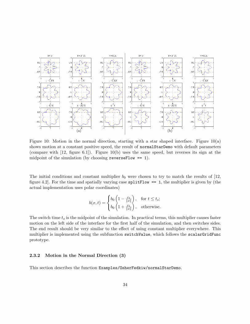
Figure 10: Motion in the normal direction, starting with a star shaped interface. Figure 10(a)shows motion at a constant positive speed, the result of normalStarDemo with default parameters(compare with [12, figure 6.1]). Figure 10(b) uses the same speed, but reverses its sign at themidpoint of the simulation (by choosing reverseFlow == 1).

The initial conditions and constant multiplier b0 were chosen to try to match the results of [12,figure 4.2]. For the time and spatially varying case splitFlow == 1, the multiplier is given by (theactual implementation uses polar coordinates)

b(x, t) =

b0(1− x1

‖x‖

), for t ≤ ts;

b0

(1 + x1

‖x‖

), otherwise.

The switch time ts is the midpoint of the simulation. In practical terms, this multiplier causes fastermotion on the left side of the interface for the first half of the simulation, and then switches sides.The end result should be very similar to the effect of using constant multiplier everywhere. Thismultiplier is implemented using the subfunction switchValue, which follows the scalarGridFuncprototype.

2.3.2 Motion in the Normal Direction (3)

This section describes the function Examples/OsherFedkiw/normalStarDemo.

34

Evolution of a star shaped interface by motion in the direction normal to the interface is shown infigure 10, and is generated by the following function, which demonstrates the use of termNormal.The subfunction switchValue contained within follows the scalarGridFunc prototype.

[ data, g, data0 ] = normalStarDemo(accuracy, reverseFlow, displayType): Demonstratesmotion in the surface normal direction at speed a(x). The accuracy and displayType pa-rameters are as normal. The boolean parameter reverseFlow specifies that the spatiallyconstant speed field should reverse direction halfway through the simulation. The initialconditions (13) are specifically designed for two dimensional grids.

The initial conditions and speed were chosen to try to match the results of [12, figure 6.1] (whenreverseFlow == 0). Note that when reverseFlow == 1 is chosen, the initial conditions are notrecovered at the final time. This loss of information occurs because of regularization along theconcave portions of the front during the first half of the simulation. For another example of thisregularization process, see section 2.4.1.

2.3.3 Normal Motion Plus Convection

This section describes the function Examples/OsherFedkiw/spinStarDemo.

Evolution of a star shaped interface by a combination of rotational convection and motion in thedirection normal to the interface is shown in figure 11. It is generated by the following function,which demonstrates the use of termSum, termNormal, and termConvection. Because termNormaland termConvection follow the schemeFunc prototype, they can be used inside of termSum.

[ data, g, data0 ] = spinStarDemo(accuracy, rigid, displayType): Demonstrates the com-bination of motion in the normal direction and convective rotation. The accuracy anddisplayType parameters are as normal. The boolean parameter rigid specifies whether therotation field should be a rigid body rotation; otherwise, it will be faster further from the ori-gin (the default behavior). The initial conditions (13) and flow fields are specifically designedfor two dimensional grids.

Although the caption of [12, figure 6.2] claims that it shows rigid body rotation, the tips of the starare clearly moving faster than the inner portions. Consequently, spinStarDemo is designed to showboth actual rigid body rotation, or to recreate the figure using a rotational speed that increases asthe square of the distance from the origin.

35

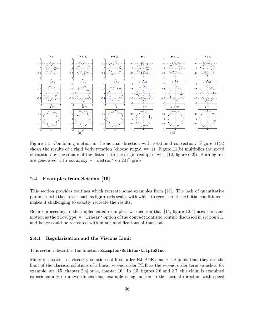
(a) (b)

Figure 11: Combining motion in the normal direction with rotational convection. Figure 11(a)shows the results of a rigid body rotation (choose rigid == 1). Figure 11(b) multiplies the speedof rotation by the square of the distance to the origin (compare with [12, figure 6.2]). Both figuresare generated with accuracy = ’medium’ on 2012 grids.

2.4 Examples from Sethian [15]

This section provides routines which recreate some examples from [15]. The lack of quantitativeparameters in that text—such as figure axis scales with which to reconstruct the initial conditions—makes it challenging to exactly recreate the results.

Before proceeding to the implemented examples, we mention that [15, figure 12.4] uses the samemotion as the flowType = ’linear’ option of the convectionDemo routine discussed in section 2.1,and hence could be recreated with minor modifications of that code.

2.4.1 Regularization and the Viscous Limit

This section describes the function Examples/Sethian/tripleSine.

Many discussions of viscosity solutions of first order HJ PDEs make the point that they are thelimit of the classical solutions of a linear second order PDE as the second order term vanishes; forexample, see [15, chapter 2.4] or [4, chapter 10]. In [15, figures 2.6 and 2.7] this claim is examinedexperimentally on a two dimensional example using motion in the normal direction with speed

36

(a) b = 0.25 (b) b = 0.025 (c) b = 0

Figure 12: The viscous limit of motion by mean curvature. All three figures show motion in thenormal direction with speed a(x) = 1− bκ(x), where each figure uses the specified value for b. Theinitial conditions are the lowest curve, and the remaining curves show the evolution of the implicitsurface at equally spaced time intervals. For b > 0, the solution remains differentiable for all time.For b = 0, the solution quickly develops kinks in the concave regions, but the result can be seen asthe limit of the differentiable solution as b→ 0. Compare with [15, figures 2.6 and 2.7]

a(x) = 1− bκ(x), where b ≥ 0 is a constant and κ(x) is the local curvature. In the case b > 0, thismotion is a combination of spatial terms (3) and (6). Figure 12 shows the attempted recreation forthree values of b. Data for the figure is generated by tripleSine, which demonstrates the use oftermNormal, termCurvature and termSum.

[ data, g, data0 ] = tripleSine(b, accuracy): Demonstrates the evolution of a sine shapedinterface under a combination of curvature and normal motion. The accuracy parameter hasthe usual options. The multiplier for the curvature dependence b must be nonnegative. Asb→ 0, this function demonstrates how motion in the normal direction is the viscous limit ofa curvature dependent motion

The difference between the b = 0.025 and b = 0 cases is subtle, and lies in the bottom of the valleysof the implicit surface: for the b = 0 case, the implicit surface quickly develops a visible sharpcorner, while the b = 0.025 case remains differentiable for all time. Lagrangian or particle basedmethods to approximate the motion of the surface in the b = 0 case would produce a “swallowtail”solution (see [15, figure 2.3]), which corresponds in some sense to a multivalued solution of the HJPDE. The upwinded derivatives used in level set methods for motion in the normal direction (thecomponent of the motion independent of κ(x)) are designed to produce this regularized and singlevalued viscosity solution, which generates an intersection free implicit surface.

37

(a) (b)

Figure 13: Motion by mean curvature of a three dimensional dumbbell, demonstrating the abilityof level set methods to easily handle the separation of implicit surfaces. Figure 13(a) shows howthe handle of the dumbbell shrinks faster due to its higher curvature, and hence the implicit surfacepinches off into two separate objects. Figure 13(b) shows contour plots at the same timesteps ona slice through the middle of the dumbbell evolving under the same motion (compare with [15,figure 14.2]).

2.4.2 Motion by Mean Curvature and Surface Separation

This section describes the function Examples/Sethian/dumbbell1.

One of the strengths of implicit surface evolution that the level set community often cites is theability to handle the merging and separation of the surfaces without any mathematical or algorith-mic effort. A classic example of the latter is evolution of the dumbbell shape under motion by meancurvature; for example, see [15, figure 14.2]. Figure 13 shows two views of the evolution. Data forthe figure is generated by dumbbell1, which demonstrates the use of termCurvature.

[ data, g, data0 ] = dumbbell1(accuracy): Demonstrates the evolution of a three dimen-sional dumbbell under motion by mean curvature. The accuracy parameter has the usualoptions. Two figures are produced: a three dimensional isosurface showing the whole dumb-bell, and a two dimensional contour of the dumbbell sliced through the middle.

38

This example also demonstrates another benefit of the implicit surface representation that is notgiven as much attention. Construction of the three dimensional dumbbell’s initial conditions isaccomplished in only four lines of code. This feat is possible because simple shapes—such asspheres, polygons and cylinders—can be created by simple mathematical functions, and unions,intersections and complements of implicitly represented sets can be accomplished by taking theminimum, maximum and negation respectively of their implicit surface functions.

As an example, the dumbbell is created by

ψleft(x) =√

(x1 + o)2 + x22 + x2

3 − r,

ψright(x) =√

(x1 − o)2 + x22 + x2

3 − r,

ψcenter(x) = max[(|x1| − o) ,

(√x2

2 + x23 − w

)],

φ(x, 0) = min [ψleft(x), ψright(x), ψcenter(x)] ,

where o is the offset of the center of the lobes of the dumbbell from the origin, r is the radius ofthe lobes, and w is the radius of the center cylinder. The left and right lobes are constructed froma spherical implicit surface function. The center portion is a cylinder aligned with the x1 axis,capped at the ends by intersection (using the max operator) with halfspaces offset from the originso as to align with the center of the lobes. The dumbbell as a whole is the union (using the minoperator) of these three implicit surfaces.

2.5 General HJ Examples from Osher & Shu [13]

This section describes functions in the directory Examples/OsherShu/.

The method for treating general Hamilton-Jacobi terms (5) adopted by this toolbox and [12] isbasically drawn from [13], and so in this section we provide code for both versions of examples 1and 2 from that paper.

2.5.1 Convex Hamiltonian (Burgers’ equation)

This section describes the function burgersLF in the directory Examples/OsherShu/, which imple-ments

Dtφ(x, t) +H(∇φ(x, t)) = 0, 1 ≤ x < 1,φ(x, 0) = − cos(πx)

(14)

39

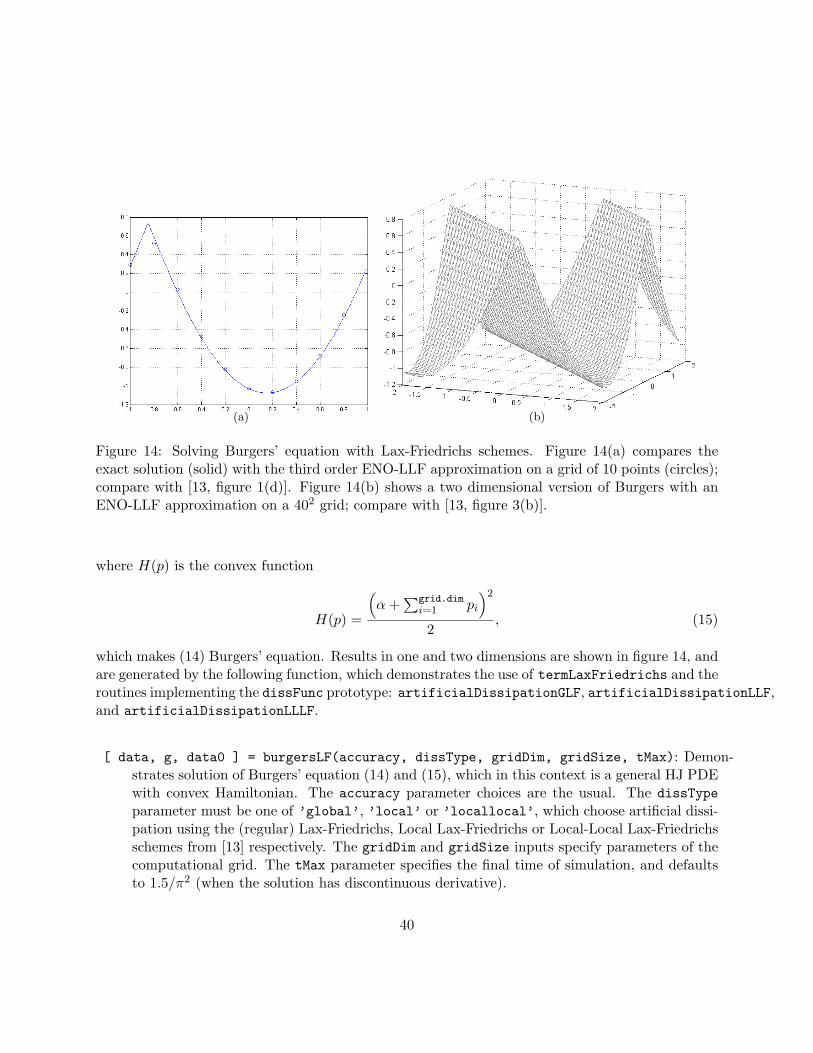
(a) (b)

Figure 14: Solving Burgers’ equation with Lax-Friedrichs schemes. Figure 14(a) compares theexact solution (solid) with the third order ENO-LLF approximation on a grid of 10 points (circles);compare with [13, figure 1(d)]. Figure 14(b) shows a two dimensional version of Burgers with anENO-LLF approximation on a 402 grid; compare with [13, figure 3(b)].

where H(p) is the convex function

H(p) =

(α+

∑grid.dimi=1 pi

)2

2, (15)

which makes (14) Burgers’ equation. Results in one and two dimensions are shown in figure 14, andare generated by the following function, which demonstrates the use of termLaxFriedrichs and theroutines implementing the dissFunc prototype: artificialDissipationGLF, artificialDissipationLLF,and artificialDissipationLLLF.

[ data, g, data0 ] = burgersLF(accuracy, dissType, gridDim, gridSize, tMax): Demon-strates solution of Burgers’ equation (14) and (15), which in this context is a general HJ PDEwith convex Hamiltonian. The accuracy parameter choices are the usual. The dissTypeparameter must be one of ’global’, ’local’ or ’locallocal’, which choose artificial dissi-pation using the (regular) Lax-Friedrichs, Local Lax-Friedrichs or Local-Local Lax-Friedrichsschemes from [13] respectively. The gridDim and gridSize inputs specify parameters of thecomputational grid. The tMax parameter specifies the final time of simulation, and defaultsto 1.5/π2 (when the solution has discontinuous derivative).

40

(a) (b)

Figure 15: Solving a non-convex general HJ PDE with Lax-Friedrichs schemes. Figure 15(a)compares the exact solution (solid) with the third order ENO-LF approximation on a grid of 10points (circles); compare with [13, figure 2(d)]. Figure 15(b) shows a two dimensional version ofthe same equation with an ENO-LF approximation on a 402 grid; compare with [13, figure 3(d)].There may be slightly more dissipation in these solutions than in those of [13] (see the discussionof nonconvexPartialFunc below).

Within the file burgersLF, the subfunction burgersHamFunc implements the hamFunc prototypefor (15). Subfunction burgersPartialFunc implements the partialFunc prototype solving (26)with Hamiltonian (15). Note that the dissipation parameter αi(x) is different from the problemparameter α.

αj(x) = maxp

∣∣∣∣∂H(p)∂pj

∣∣∣∣ = maxp

∣∣∣∣∣α+grid.dim∑

i=1

pi

∣∣∣∣∣ ,where the range over which p is optimized depends on the type of artificial dissipation chosen. For allof the types of artificial dissipation available, the range is a product of intervals, so the optimizationover p can be performed by examining each component’s interval endpoints independently.

41

2.5.2 Non-Convex Hamiltonian

This section describes the function nonconvexLF in the directory Examples/OsherShu/, whichimplements (14), where H(p) is the non-convex function

H(p) = − cos

(α+

grid.dim∑i=1

pi

). (16)

Results in one and two dimensions are shown in figure 15, and are generated by the followingfunction, which demonstrates the use of termLaxFriedrichs and the routines implementing thedissFunc prototype: artificialDissipationGLF, artificialDissipationLLF, and artificialDissipationLLLF.

[ data, g, data0 ] = nonconvexLF(accuracy, dissType, gridDim, gridSize, tMax): Demon-strates solution of (14) and (16). The accuracy parameter choices are the usual. ThedissType parameter must be one of ’global’, ’local’ or ’locallocal’, which chooseartificial dissipation using the (regular) Lax-Friedrichs, Local Lax-Friedrichs or Local-LocalLax-Friedrichs schemes from [13] respectively (although the choice turns out to be irrelevant;see the discussion of nonconvexPartialFunc below). The gridDim and gridSize inputsspecify parameters of the computational grid. The tMax parameter specifies the final time ofsimulation, and defaults to 1.5/π2 (when the solution has discontinuous derivative).

Within the file nonconvexLF, the subfunction nonconvexHamFunc implements the hamFunc proto-type for (16). Subfunction nonconvexPartialFunc implements the partialFunc prototype solv-ing (26) with Hamiltonian (16). In this version we conservatively choose

αj(x) = maxp

∣∣∣∣∂H(p)∂pj

∣∣∣∣ = maxp

∣∣∣∣∣sin(α+

grid.dim∑i=1

pi

)∣∣∣∣∣ ≤ 1

as an upper bound on the maximum of the magnitude of the partials. This choice is not particularlyaccurate, but it will maintain numerical stability. Because it does not depend on the range of p,all of the dissipation methods will give the same result.

2.6 Examples of Reachable Sets

As engineering systems have become more complex, a formal methods community has developedto study methods of validating or verifying the correct behavior of such systems. Model checkingis one major thrust of this community, and is a verification method in which the state space of the

42

design is explored in order to determine whether the system—or at least its mathematical model—can enter into an unsafe or incorrect state. Many model checking algorithms attempt to computea reachable set, which comes in two flavors. The forwards reachable set is the set of states thatcan be reached by system trajectories which start in a given set of initial states. The backwardsreachable set is the set of states that can give rise to trajectories which subsequently pass throughsome given set of target states. In [18, 7, 9] we developed a method of computing robust backwardsreachable sets for nonlinear continuous and hybrid systems using an HJ PDE. For more discussionof reachable sets and alternative algorithms for their computation, we suggest [9] and the referencescontained therein.

This toolbox contains several examples of script files to compute reachable sets. We have notyet created an automatic method of computing reachable sets from a Simulink block diagram orMatlab m-file description of a system. Instead, we outline the steps needed to encode a reachableset computation as an HJ PDE in the toolbox.

Consider first the backwards reachable set from a target set T of a continuous system with dynamicsx = f(x, a, b), where x ∈ Rn is the state of the system, T ⊂ Rn, a ∈ A ⊂ Rna is an input seeking tokeep the system from entering T , and b ∈ B ⊂ Rnb is an input seeking to drive the system into T .In many examples, T is an unsafe set so that a should be considered controls keeping the systemsafe, and b consists of disturbances or model uncertainties which are assumed to try to make thesystem unsafe (a robust but conservative treatment). In some examples a and/or b may not bepresent.

Computation of the backwards reachable set is normally encoded as a terminal value HJ PDE—thesame as an initial value PDE, but time runs backwards. The terminal value encodes the target set,so φ(x, 0) should be an implicit surface function representation of T . Evolution of the backwardsreachable set is accomplished by solving

Dtφ(x, t) + min[0,H(x,Dxφ(x, t))] = 0 (17)

backwards in time, whereH(x, p) = max

a∈Aminb∈B

pT f(x, a, b). (18)

The solution φ(x, t) is an implicit surface representation of the finite time backwards reachable set.While the toolbox is designed for solving initial value and not terminal value PDEs, for autonomoussystems (f does not depend on t) converting to the initial value PDE form used in the toolboxsimply requires multiplying f by -1.

Consideration of (17) reveals that the minimization with zero component is equivalent to constrain-ing the sign of the temporal derivative to be positive (10). This constraint keeps the reachable setfrom shrinking as time progresses, and is implemented with the spatial term approximation routinetermRestrictUpdate, which appears in all of the examples below.

43

If the model involves no inputs or nondeterministic parameters, then (18) degenerates to convectionunder flow field v(x) = f(x) and can be treated as an example of the form (2). This type ofcontinuous dynamics is encountered in section 2.6.3—although the discrete part of this system hasinputs, the continuous part (which gives rise to the HJ PDE) does not. However, most cases involveat least one of the inputs a or b, and so (18) must be treated as a general Hamiltonian (5) usingtermLaxFriedrichs. The other examples in this section involve inputs and consequently requirethe latter treatment.

As described in section 3.6.2, use of termLaxFriedrichs requires providing functions which satisfythe derivFunc, dissFunc, hamFunc, and partialFunc prototypes. The first is chosen from amongthe upwind approximations of the first derivative described in section 3.4.1. The second is chosenfrom among the artificial dissipation functions described in section 3.6.2. The final two must beprovided by the user.

The function satisfying the hamFunc prototype must compute the solution of (18). Since theoptimization over inputs a and b is done for fixed x and p = ∇φ(x, t), it can often be performedexactly. If exact optimization over the continuous ranges of A and/or B is not possible, theycan be sampled discretely. However, users should keep in mind that if H is overestimated—forexample, if the truly optimal value of b is not found—then the reachable set will be underestimated.Furthermore, care should be taken if the effects of a and b are not separable. In that case, the orderof the optimizations in (18) demands that the value of a be fixed before the minimization over b isperformed (a robust but conservative choice if a is the controls and b is the disturbances).

Coding the function satisfying the partialFunc prototype is often the most challenging part ofcomputing a reachable set. This function must solve (26), which in this context translates to

αi(x) = maxp

∣∣∣∣∂H(x, p)∂pi

∣∣∣∣ = maxp

∣∣∣∣maxa∈A minb∈B pT f(x, a, b)

∂pi

∣∣∣∣ , (19)

where the hyperrectangular range over which p is optimized is an argument to partialFunc. Theorder of the optimizations cannot be modified. Underestimation of this value can lead to numericalinstability and toolbox failure. Overestimation will lead to a numerically benign increase in theamount of artificial dissipation introduced by the Lax-Friedrichs approximation. Such dissipationwill round sharp corners in the reachable set and, in the worst case, may cause its underestimation;however, since the optimization in (19) can rarely be performed exactly, overestimation is thepreferable form of error.

Before proceeding to specific examples, we examine the mathematics of a particularly commonform of dynamics. A nonlinear system’s inputs enter linearly if we can separate its dynamics intothe form

f(x, a, b) = fx(x) + Fa(x)a+ Fb(x)b, (20)

44

where fx : Rn → Rn, Fa : Rn → Rna×n and Fb : Rn → Rnb×n.† We also assume that the inputconstraints are hyperrectangles

ai ∈ Ai = [Ai,Ai], A =na∏i=1

Ai,

bi ∈ Bi = [Bi,Bi], B =na∏i=1

Bi.

Then the optimal inputs to the Hamiltonian (18) can be determined analytically

a∗i (x, p) =

{Ai, if

∑nj=1 pjFa

ji(x) ≤ 0;Ai otherwise;

b∗i (x, p) =

{Bi, if

∑nj=1 pjFb

ji(x) ≤ 0;Bi otherwise.

(21)

Futhermore, defining

Amaxi = max

(|Ai| ,

∣∣Ai

∣∣) , Bmaxi = max

(|Bi| ,

∣∣Bi

∣∣) ,the terms (19) for the partialFunc routine can be slightly overestimated by

αj(x) ≤∣∣fx

j (x)∣∣+ na∑

i=1

∣∣Faji(x)

∣∣Amaxi +

nb∑i=1

∣∣∣Fbji(x)

∣∣∣Bmaxi . (22)

Section 2.6.1 examines a system which satisfies these separability assumptions.

The extension to hybrid system reachable sets is very much an ad hoc process in the current toolbox.The discrete iteration proposed in [17] and repeated with minor modifications in [18, 9] can be codedmanually into an m-file, as is done in section 2.6.3. The avoid portion of the reach-avoid operator isimplemented by masking the evolving reachable set against the escape set using the PostTimestepoption of the odeCFLn integrators. For autonomous systems, we no longer believe that the escapeset itself need be evolved. A revised hybrid system reachable set algorithm—based on variationalinequalities—is under development and will be integrated into the toolbox once it is complete.

†Linear systems clearly satisfy this property, since in that case fx(x) = Ax where A ∈ Rn×n, while Fa and Fb

are constant matrices.

45

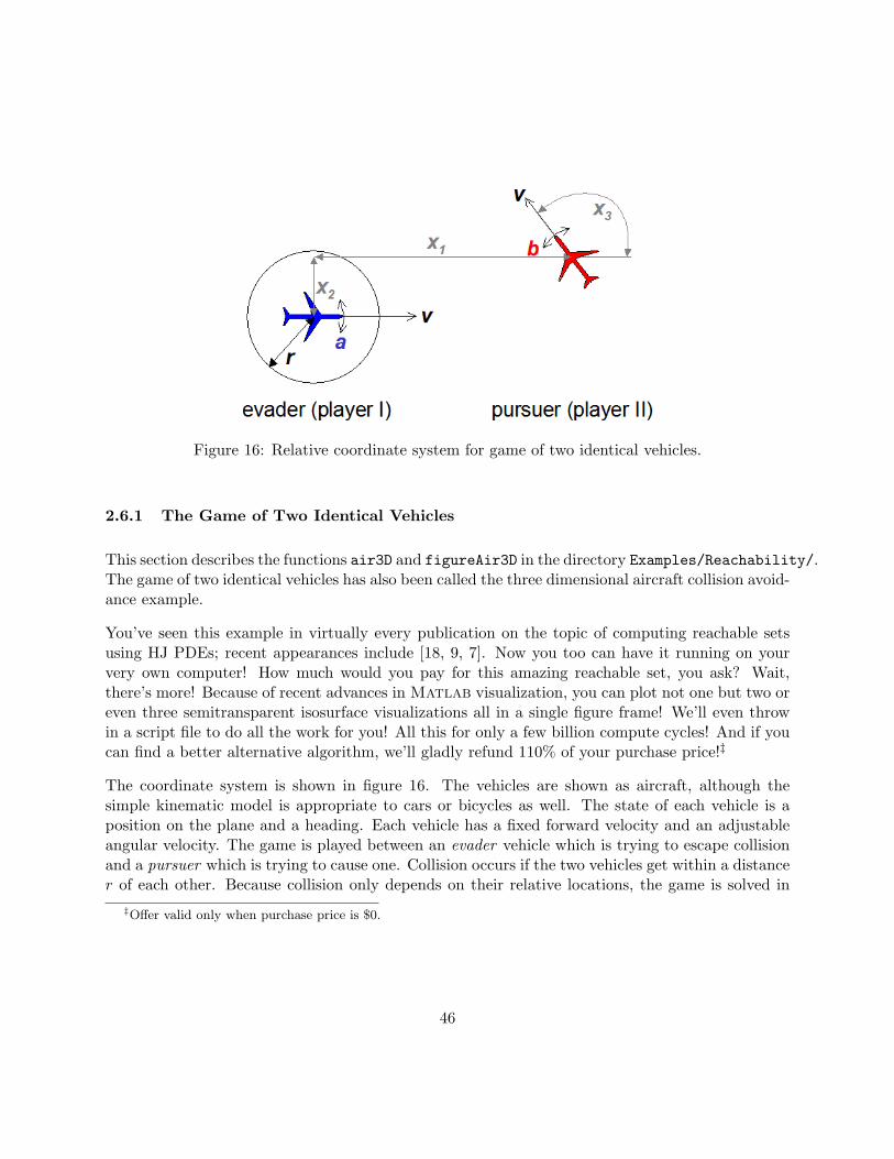
Figure 16: Relative coordinate system for game of two identical vehicles.

2.6.1 The Game of Two Identical Vehicles

This section describes the functions air3D and figureAir3D in the directory Examples/Reachability/.The game of two identical vehicles has also been called the three dimensional aircraft collision avoid-ance example.

You’ve seen this example in virtually every publication on the topic of computing reachable setsusing HJ PDEs; recent appearances include [18, 9, 7]. Now you too can have it running on yourvery own computer! How much would you pay for this amazing reachable set, you ask? Wait,there’s more! Because of recent advances in Matlab visualization, you can plot not one but two oreven three semitransparent isosurface visualizations all in a single figure frame! We’ll even throwin a script file to do all the work for you! All this for only a few billion compute cycles! And if youcan find a better alternative algorithm, we’ll gladly refund 110% of your purchase price!‡

The coordinate system is shown in figure 16. The vehicles are shown as aircraft, although thesimple kinematic model is appropriate to cars or bicycles as well. The state of each vehicle is aposition on the plane and a heading. Each vehicle has a fixed forward velocity and an adjustableangular velocity. The game is played between an evader vehicle which is trying to escape collisionand a pursuer which is trying to cause one. Collision occurs if the two vehicles get within a distancer of each other. Because collision only depends on their relative locations, the game is solved in

‡Offer valid only when purchase price is $0.

46

(a) (b)

Figure 17: The target and reachable sets for the game of two identical vehicles as visualizedby figureAir3D. Figure 17(a) shows the target cylinder representing the set of collision states.Figure 17(b) shows the final reachable set at t = 2.8, computed by air3D(’medium’).

relative coordinates with the evader fixed at the origin facing right. The target set T is the set ofcollided states, which is a cylinder of radius r centered on the x3 axis. The relative dynamics are

x =d

dt

x1

x2

x3

=

−va + vb cosx3 + ax2

vb sinx3 − ax1

b− a

= f(x, a, b), (23)

where va ∈ R is the fixed linear velocity of the evader, vb ∈ R is the fixed linear velocity of thepursuer, a ∈ A ⊂ R is the angular velocity of the evader and is the “control” input trying to avoid T ,and b ∈ B ⊂ R is the angular velocity of the pursuer and is the “disturbance” input trying to reachT . The routines below assume va > 0, vb > 0, A = [−Amax,Amax], Amax > 0, B = [−Bmax,Bmax]and Bmax > 0, although the algorithm will work for any combination of parameters. In particular,if va = vb and Amax = Bmax, then the two vehicles are considered identical.

The reachable set for the game of two identical vehicles with r = 5, va = vb = 5 and Amax = Bmax =1 is shown in figure 17. The data for the figure is generated by the following function, which demon-strates the use of termLaxFriedrichs and termRestrictUpdate. Because termLaxFriedrichsfollows the schemeFunc prototype, it can be used inside of termRestrictUpdate.

[ data, g, data0 ] = air3D(accuracy): Demonstrate the (now infamous) three dimensionalreachable set for the game of two identical vehicles. The accuracy parameter is as usual.The vehicle parameters and visualization technique can be modified within the m-file.

47

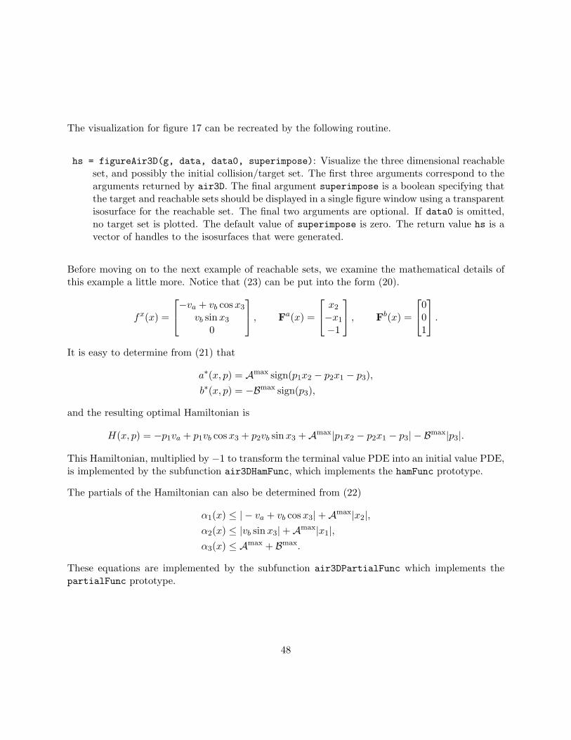
The visualization for figure 17 can be recreated by the following routine.

hs = figureAir3D(g, data, data0, superimpose): Visualize the three dimensional reachableset, and possibly the initial collision/target set. The first three arguments correspond to thearguments returned by air3D. The final argument superimpose is a boolean specifying thatthe target and reachable sets should be displayed in a single figure window using a transparentisosurface for the reachable set. The final two arguments are optional. If data0 is omitted,no target set is plotted. The default value of superimpose is zero. The return value hs is avector of handles to the isosurfaces that were generated.

Before moving on to the next example of reachable sets, we examine the mathematical details ofthis example a little more. Notice that (23) can be put into the form (20).

fx(x) =

−va + vb cosx3

vb sinx3

0

, Fa(x) =

x2

−x1

−1

, Fb(x) =

001

.It is easy to determine from (21) that

a∗(x, p) = Amax sign(p1x2 − p2x1 − p3),b∗(x, p) = −Bmax sign(p3),

and the resulting optimal Hamiltonian is

H(x, p) = −p1va + p1vb cosx3 + p2vb sinx3 +Amax|p1x2 − p2x1 − p3| − Bmax|p3|.

This Hamiltonian, multiplied by −1 to transform the terminal value PDE into an initial value PDE,is implemented by the subfunction air3DHamFunc, which implements the hamFunc prototype.

The partials of the Hamiltonian can also be determined from (22)

α1(x) ≤ | − va + vb cosx3|+Amax|x2|,α2(x) ≤ |vb sinx3|+Amax|x1|,α3(x) ≤ Amax + Bmax.

These equations are implemented by the subfunction air3DPartialFunc which implements thepartialFunc prototype.

48

Figure 18: Evolution of the acoustic capture game’s reachable set.

2.6.2 Acoustic Capture

This section describes the function Examples/Reachability/acoustic.

The example is a variation of the classical homicidal chauffer problem. The version of the gamestudied here is taken from [2] and we recreate the results in [9]. The reachable set is calculated inrelative coordinates with the pursuer fixed at the origin, leading to dynamics

d

dt

[xy

]= Wp

[0−1

]+Wp

R

[y−x

]b+ 2We min

(√x2 + y2, S

)a = f(z, a, b), (24)

where the state is z = (x, y) ∈ R2 and the problem parameters are the pursuer’s speed Wp, theevader’s speed We, the pursuer’s turn radius R and the evader’s radius of maximum speed S. Theinput constraints a ∈ A and b ∈ B are

A = {a ∈ R2 | ‖a‖ ≤ 1} ⊂ R2 B = [−1,+1] ⊂ R.

The pursuer’s capture set T is a wide but shallow horizontal rectangle near the origin.

49

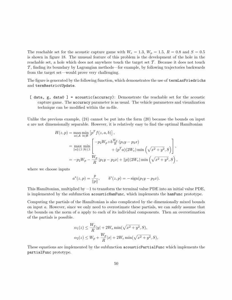
The reachable set for the acoustic capture game with We = 1.3, Wp = 1.5, R = 0.8 and S = 0.5is shown in figure 18. The unusual feature of this problem is the development of the hole in thereachable set, a hole which does not anywhere touch the target set T . Because it does not touchT , finding its boundary by Lagrangian methods—for example, by following trajectories backwardsfrom the target set—would prove very challenging.

The figure is generated by the following function, which demonstrates the use of termLaxFriedrichsand termRestrictUpdate.

[ data, g, data0 ] = acoustic(accuracy): Demonstrate the reachable set for the acousticcapture game. The accuracy parameter is as usual. The vehicle parameters and visualizationtechnique can be modified within the m-file.

Unlike the previous example, (24) cannot be put into the form (20) because the bounds on inputa are not dimensionally separable. However, it is relatively easy to find the optimal Hamiltonian

H(z, p) = maxa∈A

minb∈B

[pT f(z, a, b)

],

= max‖a‖≤1

min|b|≤1

−p2Wp+bWp

R (p1y − p2x)

+ (pTa)(2We) min(√

x2 + y2, S) ,

= −p2Wp −Wp

R|p1y − p2x|+ ‖p‖(2We) min

(√x2 + y2, S

),

where we choose inputs

a∗(z, p) =p

‖p‖, b∗(z, p) = − sign(p1y − p2x).

This Hamiltonian, multiplied by −1 to transform the terminal value PDE into an initial value PDE,is implemented by the subfunction acousticHamFunc, which implements the hamFunc prototype.

Computing the partials of the Hamiltonian is also complicated by the dimensionally mixed boundson input a. However, since we only need to overestimate these partials, we can safely assume thatthe bounds on the norm of a apply to each of its individual components. Then an overestimationof the partials is possible.

α1(z) ≤Wp

R|y|+ 2We min(

√x2 + y2, S),

α2(z) ≤Wp +Wp

R|x|+ 2We min(

√x2 + y2, S),

These equations are implemented by the subfunction acousticPartialFunc which implements thepartialFunc prototype.

50

Figure 19: Hybrid automata for the three mode protocol.

2.6.3 Multimode Collision Avoidance

This section describes the function Examples/Reachability/airMode.

As an example of a hybrid system reachable set we take the three mode collision avoidance examplefrom [8, 9]. Like the game of two identical vehicles in section 2.6.1, this is a collision avoidancescenario played with two simple kinematic vehicles. In this case, however, the angular velocitiesof the two vehicles are fixed and equal, so that their relative angle never varies. Therefore thecomputation can be performed in two dimensions.

The hybrid automata for the example is shown in figure 19. The only input to the system is thedecision σ to initiate the collision avoidance protocol, and after that point all switches and motionis synchronized between the vehicles. The relative location of the vehicles always follows one of twodynamics:

• Straight motion: both vehicles move with constant linear velocities and zero angular velocities.The dynamics are

z =d

dt

[xr

yr

]=[−va + vb cosψr

va sinψr

]= fs(z),

where va and vb are fixed (although not necessarily equal).

51

Figure 20: Reachable set in the first mode for the three mode collision avoidance protocol. Thesolid region is the set of states within which collision is inevitable. Outside the solid contour theprotocol can be safely initiated. The dashed contour shows the edges of the unsafe set if no protocolis initiated.

• Curved motion: both vehicles move with constant linear velocities and a constant, equalangular velocity. The dynamics are

z =d

dt

[xr

yr

]=[−va + vb cosψr + ωyr

va sinψr − ωxr

]= fc(z),

where va, vb and ω are fixed.

Because the continuous dynamics involve no inputs, we can simplify the computation by usingconvection by constant flow fields within each of the individual modes.

The reachable set for this multimode protocol with va = 3, vb = 4, ψ = −4π/3 and ω = 1 isshown in figure 20. The figure is generated by the following function, which demonstrates the useof termConvection and termRestrictUpdate.

52

[ reach, g, avoid, data0 ] = airMode(accuracy): Demonstrate the three mode collisionavoidance protocol reach set computation. The accuracy parameter is as usual. The ve-hicle parameters and visualization technique can be modified within the m-file. The returnparameter reach is an implicit surface function for the set of states where a collision is in-evitable, and the parameter avoid is an implicit surface function for the set of states in whichthe protocol can be safely initiated.

The computation of the reach sets in each individual mode is relatively straightforward (all the moreso because of the convective dynamics), and is accomplished by the subfunction findReachSet. Thetricky and entirely ad hoc component is how to keep track of the interaction between the modes.For this specific example, four reach set computations are performed.

• The set of states which lead to collision in the final mode. This is simple convection of thetarget set (a circle) according to the constant linear velocity dynamics fs.

• The set of states which lead to collision in the second mode. This is simple convection of thetarget set according to a constant rotational flow field fc.

• The set of states which, when rotated through the second mode, lead to collision in thethird mode. This set is computed starting with the third mode’s unsafe states and using therotational flow field fc. However, this computation does not restrict the sign of the temporalderivative in the HJ PDE. Such a restriction would mark states as unsafe if they merelypassed into and then out of the third mode’s unsafe states while still in the protocol’s secondmode. Instead, states should only be marked as unsafe if they pass through the collision setin the second mode, or switch into the third mode while in the third mode’s unsafe states.

• The set of states in which a collision is inevitable whether the protocol is initiated or not. Thiscomputation involves the reach-avoid operator. The escape set is all those states in which itis safe to initiate the protocol; specifically, the complement of the union of the states whichlead to collision in the second mode (the second reach set computed) and the states which gothrough the second mode and lead to collision in the third (the third reach set computed).This escape set is used to mask the evolution of the reach set via a constraint of the form (11)The reach set’s evolution is otherwise identical to the evolution in the third mode above.The masking is performed by postTimestepMask, which implements the postTimestepFuncprotocol.

For more general reach and reach-avoid computation algorithms, see [18] and the citations within.

2.7 Testing Routines

This section describes functions in Examples/Test.

53

2.7.1 Initial Conditions

Several script-like functions were written to test the initial condition routines for basic shapes andset operations for constructive solid geometry (see section 3.3).

initialConditionsTest1D(): Creates a sequence of shapes defined by implicit surface functionsin a one dimensional state space. In one dimension, an implicitly defined shape is always aninterval, although one or both endpoints may be infinite. Plotting the intervals is not terriblyexciting, so the entire implicit surface function for each shape is displayed as a function plot,state vs function value. The implicitly defined interval for each plot is the region in whichthe function value is negative.

initialConditionsTest2D(): Creates a sequence of shapes defined by implicit surface functionsin a two dimensional state space. The two dimensional implicit surfaces are shown in onefigure window by contour plots, while the implicit surface functions themselves appear in aseparate window as surface plots.

initialConditionsTest3D(): Creates a sequence of shapes defined by implicit surface functionsin a three dimensional state space. The three dimensional implicit surfaces are shown as iso-surfaces, because the implicit surface functions themselves are rather challenging to visualize.

2.7.2 Derivative Approximations

Do the high resolution (high order) approximation schemes live up to their billing? A pair of routineswere designed to test the functions (see section 3.4.1) and determine their errors, convergence ratesand execution times. Given proper input data, solutions of the time-dependent HJ PDEs thatwe solve with this toolbox should remain continuous, although they may not be differentiableeverywhere. In order to test whether the approximation schemes correctly handle this situation,the test function is chosen to be continuous but with discontinuities in the derivative.

[ errorL, errorR, time ] = firstDerivSpatialTest1(scheme, dim, whichDim, dx): Com-putes the errors in the left and right approximations for a single scheme on a single grid. Thescheme is specified by the function handle scheme. The dim dimensional grid has periodicboundary conditions in every dimension and grid spacing dx. The derivative is taken in di-mension whichDim. Letting xd be the whichDim component of the state vector x, the testfunction is

f(x) =

sin(2πxd + π

4

), for 0 ≤ xd <

14 ;

sin(2πxd − π

4

), for 1

4 ≤ xd <12 ;

sin (2πxd) + 1, for 12 ≤ xd < 1.

54

(a) (b)

(c) (d)

Figure 21: Examples of implicitly defined surfaces and sets built by constructive solid geometryoperations from basic shapes. The top row is generated by initialConditionsTest2D and thebottom row by initialConditionsTest3D. Figure 21(a) shows a square subtracted from a circle,while figure 21(b) shows a nonconvex polygon constructed by intersections and unions of hyper-planes. Figure 21(c) shows the union of a sphere and a cube, and figure 21(d) shows an octohedronconstructed by the intersection of eight hyperplanes.

55

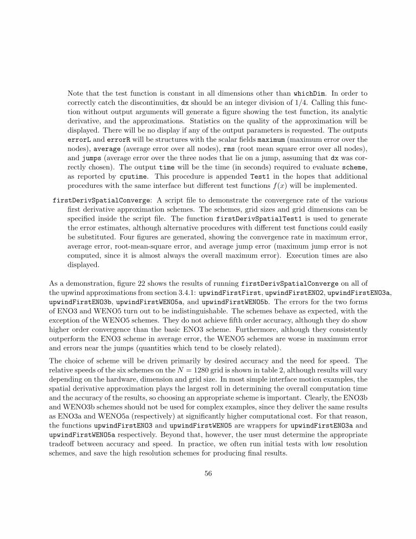
Note that the test function is constant in all dimensions other than whichDim. In order tocorrectly catch the discontinuities, dx should be an integer division of 1/4. Calling this func-tion without output arguments will generate a figure showing the test function, its analyticderivative, and the approximations. Statistics on the quality of the approximation will bedisplayed. There will be no display if any of the output parameters is requested. The outputserrorL and errorR will be structures with the scalar fields maximum (maximum error over thenodes), average (average error over all nodes), rms (root mean square error over all nodes),and jumps (average error over the three nodes that lie on a jump, assuming that dx was cor-rectly chosen). The output time will be the time (in seconds) required to evaluate scheme,as reported by cputime. This procedure is appended Test1 in the hopes that additionalprocedures with the same interface but different test functions f(x) will be implemented.

firstDerivSpatialConverge: A script file to demonstrate the convergence rate of the variousfirst derivative approximation schemes. The schemes, grid sizes and grid dimensions can bespecified inside the script file. The function firstDerivSpatialTest1 is used to generatethe error estimates, although alternative procedures with different test functions could easilybe substituted. Four figures are generated, showing the convergence rate in maximum error,average error, root-mean-square error, and average jump error (maximum jump error is notcomputed, since it is almost always the overall maximum error). Execution times are alsodisplayed.

As a demonstration, figure 22 shows the results of running firstDerivSpatialConverge on all ofthe upwind approximations from section 3.4.1: upwindFirstFirst, upwindFirstENO2, upwindFirstENO3a,upwindFirstENO3b, upwindFirstWENO5a, and upwindFirstWENO5b. The errors for the two formsof ENO3 and WENO5 turn out to be indistinguishable. The schemes behave as expected, with theexception of the WENO5 schemes. They do not achieve fifth order accuracy, although they do showhigher order convergence than the basic ENO3 scheme. Furthermore, although they consistentlyoutperform the ENO3 scheme in average error, the WENO5 schemes are worse in maximum errorand errors near the jumps (quantities which tend to be closely related).

The choice of scheme will be driven primarily by desired accuracy and the need for speed. Therelative speeds of the six schemes on theN = 1280 grid is shown in table 2, although results will varydepending on the hardware, dimension and grid size. In most simple interface motion examples, thespatial derivative approximation plays the largest roll in determining the overall computation timeand the accuracy of the results, so choosing an appropriate scheme is important. Clearly, the ENO3band WENO3b schemes should not be used for complex examples, since they deliver the same resultsas ENO3a and WENO5a (respectively) at significantly higher computational cost. For that reason,the functions upwindFirstENO3 and upwindFirstWENO5 are wrappers for upwindFirstENO3a andupwindFirstWENO5a respectively. Beyond that, however, the user must determine the appropriatetradeoff between accuracy and speed. In practice, we often run initial tests with low resolutionschemes, and save the high resolution schemes for producing final results.

56

(a) Maximum error. (b) Average error.

(c) Average error at derivative discontinuities. (d) Root mean square error.

Figure 22: Convergence rates demonstrated by the various upwind approximations of the firstderiviative from section 3.4.1, as generated by firstDerivSpatialConverge on the test functionin firstDerivSpatialTest1 in two dimensions. The short lines in the middle of the bottom ofeach figure show the slopes corresponding to first, second, third and fifth order convergence.

57

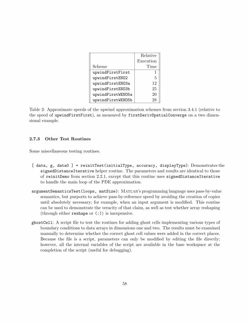
RelativeExecution

Scheme TimeupwindFirstFirst 1upwindFirstENO2 5upwindFirstENO3a 12upwindFirstENO3b 25upwindFirstWENO5a 20upwindFirstWENO5b 28

Table 2: Approximate speeds of the upwind approximation schemes from section 3.4.1 (relative tothe speed of upwindFirstFirst), as measured by firstDerivSpatialConverge on a two dimen-sional example.

2.7.3 Other Test Routines

Some miscellaneous testing routines.

[ data, g, data0 ] = reinitTest(initialType, accuracy, displayType): Demonstrates thesignedDistanceIterative helper routine. The parameters and results are identical to thoseof reinitDemo from section 2.2.1, except that this routine uses signedDistanceIterativeto handle the main loop of the PDE approximation.

argumentSemanticsTest(loops, matSize): Matlab’s programming language uses pass-by-valuesemantics, but purports to achieve pass-by-reference speed by avoiding the creation of copiesuntil absolutely necessary; for example, when an input argument is modified. This routinecan be used to demonstrate the veracity of that claim, as well as test whether array reshaping(through either reshape or (:)) is inexpensive.

ghostCell: A script file to test the routines for adding ghost cells implementing various types ofboundary conditions to data arrays in dimensions one and two. The results must be examinedmanually to determine whether the correct ghost cell values were added in the correct places.Because the file is a script, parameters can only be modified by editing the file directly;however, all the internal variables of the script are available in the base workspace at thecompletion of the script (useful for debugging).

58

3 Code Components

This section discusses the routines in the directory Kernel. It is designed primarily as a reference,although the best reference is probably the help entries for the routines themselves, which are foundat the top of each function’s source m-file and can be accessed with Matlab’s help command.

3.1 Grids

This section discusses functions found in the directory Kernel/Grids.

The goal of this toolbox is to allow simple solution of simple interface motion problems. Becausethe computational grid affects virtually every operation in a hyperbolic PDE solver, nowhere is thedecision to pursue simplicity over generality more defining than in our choice of grids. While thereare many problems that cannot be solved to high accuracy or within reasonable computational timewithout resorting to adaptive and/or unstructured grids, the complexity of the data structures forsuch grids makes them poorly suited for simple problems or the Matlab interpreted programmingenvironment.

Consequently, we have adopted a very simple grid structure: a fixed rectangular Euclidean mesh.The grid cells are of fixed size, although the spacing for each dimension may be chosen indepen-dently. A grid is represented by a structure with fields:

grid.dim: The dimension of the grid. Typically between one and four, although the code shouldwork in any dimension.

grid.min: A column vector specifying the lower left corner of the computational domain.

grid.max: A column vector specifying the upper right corner of the computational domain.

grid.bdry: A cell column vector. Each element is a function handle pointing to the bound-ary condition (see section 3.2), which provides data values for nodes which fall outside thecomputational domain in that dimension.

grid.bdryData: A cell column vector. Each element provides parameters for the correspondinggrid.bdry element.

grid.N: A column vector specifying the number of grid nodes in each dimension.

grid.dx: A column vector specifying the grid cell spacing in each dimension.

59

grid.vs: A cell column vector. Each element contains a regular column vector giving the node lo-cations in the corresponding dimension. Generated by grid.vs{d} = linspace(grid.min(d),grid.max(d), grid.N(d)).

grid.xs: A cell column vector. Each element contains an array giving the node locations for eachnode in the entire grid. Generated by [ grid.xs{1:grid.dim} ] = ndgrid(grid.vs{:}).

grid.axis: A row vector specifying the computational domain boundary in a format suitable topass to Matlab’s axis command.

grid.shape: A row vector specifying the number of nodes in each dimension in a format suitableto pass to Matlab’s reshape command. Specifically

grid.shape =

{[grid.N 1], if grid.dim = 1;grid.N′, otherwise.

If data is a data array defined on grid, then grid.shape == size(data).

Notice that manually entering all of these fields would be tedious and prone to inconsistencies.Therefore, most will be automatically generated by a call to processGrid. Typically, only thefields grid.dim, grid.min, grid.max, grid.bdry, grid.bdryData and one of grid.N or grid.dxneed be supplied by the user.

gridOut = processGrid(gridIn, data): Fill in the fields missing from a grid structure. Wherepossible, missing fields in gridIn will be automatically generated. Some consistency checkingis also performed on the fields that already exist. Some fields have default values, which canbe seen in the help entry. This function can be safely called multiple times on the same gridstructure (the second call will only invoke consistency checks), although it can be rather slowto execute. The optional second argument is only checked to ensure that ndims(data) andsize(data) are consistent with gridIn.dim and gridIn.N respectively.

The user should ensure that processGrid is called before a grid structure is passed into any ofthe other routines in this toolbox. The resulting grid will be a grid.dim dimensional array withgrid.N(d) nodes in dimension d. Notice that the grid.xs field will generally be much largerthan any other, since it will have a total of grid.dim * prod(grid.N) entries. While it is large,alternative schemes for vectorizing the level set computations inevitably lead to allocating multiplecopies of similarly large state arrays at different levels in the call stack, and so it was decided toinclude this single copy of the state array in the grid structure. The large size of this field will notreduce computational efficiency as long as the grid structure and its fields are not modified withinany of the functions to which it is passed; so far we have found no reason to do so within any ofour examples. When saving a grid to disk, the command grid = rmfield(grid, ’xs’); can beused to remove this field and hence enormously reduce the size of the resulting file. The field canbe easily regenerated after a load by another call to processGrid.

60

3.2 Boundary Conditions

This section discusses functions found in the directory Kernel/BoundaryCondition.

The computational domain is finite, and so the finite difference stencils we use to approximate thespatial derivatives of the HJ PDE will extend beyond the edge of the grid when working on nodesnear that edge. In order to manage this process, every face of the computational domain must beassociated with a boundary condition. This association is represented by function handles passedin the grid.bdry field of the grid structure described in section 3.1. In general, each dimensioncan have its own boundary conditions, although the upper and lower boundaries in a particulardimension must use the same boundary condition function.

The boundary condition functions are called by the spatial derivative approximations (see sec-tion 3.4). When called for a particular dimension, they add an appropriate number of ghostnodes—the stencil width specified by the spatial derivative approximation—to the upper and lowersides of the data array in that dimension. The values placed in these ghost nodes are determinedby the type of boundary condition.

addGhostPeriodic: Values from the lower end of the array are copied to the upper ghost nodes,and vice versa. This boundary condition requires no additional parameters.

addGhostDirichlet: A constant value is placed into the ghost nodes. Different constants may bechosen for the upper and lower ghost nodes. The values are passed as parameters.

addGhostNeumann: The ghost nodes are filled with data linearly extrapolated from the com-putational boundary so as to have a constant specified derivative normal to the boundary.Different constants may be chosen for the upper and lower ghost nodes. The constants arepassed as parameters.

addGhostExtrapolate: The ghost nodes are filled with data linearly extrapolated from the com-putational boundary so as to have a slope towards or away from the zero level set. Thechoice of towards or away from the zero level set is passed as a parameter. While this is nota traditional PDE boundary condition, it proves quite useful in level set computations fordomains with inflow boundaries that have no physically appropriate boundary conditions. Bychoosing to extrapolate away from zero, the ghost cells will never falsely imply the existenceof a “ghost” interface beyond the computational domain, and hence lend stability to a po-tentially unstable nonphysical computational domain boundary. All of the examples use thisboundary condition when the periodic boundary condition cannot be justified.

For more details on the parameters required by each boundary condition function, see the indi-vidual help entries. All four boundary condition functions use the same call structure, which wedemonstrate with addGhostExtrapolate.

61

dataOut = addGhostExtrapolate(dataIn, dim, width, ghostData): Adds width ghost cellsin dimension dim to the top and bottom of the data array dataIn. These ghost cells are filledwith data linearly extrapolated from the two nodes nearest the boundary in the appropriatedimension. The sign of the extrapolation is chosen so as to extrapolate away from or towardsthe zero level set, as specified by the boolean field ghostData.towardZero (defaults to false).For example, if dataIn is two dimensional of size grid.shape, then dim = 2, width = 1 andghostData.towardZero = 0 would result in a two dimensional dataOut of size grid.shape+ [ 0, 2 ]T with values generated by

dataOut(:, 1) =dataIn(:, 1)+ sign(dataIn(:, 1))|dataIn(:, 1)− dataIn(:, 2)|

dataOut(:, 2 : end− 1) =dataIn(:, 1 : end)dataOut(:, end) =dataIn(:, end)

+ sign(dataIn(:, end))|dataIn(:, end)− dataIn(:, end− 1)|

Function handles to the boundary condition functions described above are passed as the elementsof the cell vector grid.bdry of the grid structure. Each is called on a single dimension at a time.While this one dimension at a time method reduces the memory requirements of adding ghost cellswhen working with the one dimension at a time first order spatial derivative approximations insection 3.4.1, it is sometimes necessary to create ghost cells on every side of the data array at once.Two helper routines are provided for this purpose.

dataOut = addGhostAllDims(grid, dataIn, width): Adds width ghost cells to the top andbottom of every dimension of the data array dataIn, according to the boundary conditionsspecified in grid.bdry.

[ vs, xs ] = addNodesAllDims(grid, width): Creates vs and xs cell vectors that correspondto those in grid.vs and grid.xs, but include the states of all the ghost nodes as well as theregular grid nodes. Note that xs can be very large, and hence this function can be expensiveto evaluate.

The process of creating and releasing the memory for the ghost nodes at each timestep is clearlynot the most efficient way to handle boundary conditions. Unfortunately, the alternative would beto preallocate sufficient memory in the data array for the ghost cells. The size of the preallocationwould depend on the spatial derivative approximation, and would necessitate an offset indexingsystem to retrieve the true data from the array. Thus, we decided to use the slower method ofrepetitive ghost cell allocation rather than destroy the intuitively simple layout of the data array.A future object oriented version of this toolbox may be able to revisit this decision and achieveboth goals with a single implementation.

62

3.3 Initial Conditions

This section describes functions in Kernel/InitialConditions.

A major advantage of implicit surface representations is the ease with which complex shapes canbe created through operations from constructive solid geometry. Simple algebraic functions cancreate implicit surface functions for basic shapes—circles, spheres, cylinders, squares, cubes, rect-angles, hyperplanes, and polygons, to name just a few. These shapes can then be combined byunions, intersections, complements and set differences to form more complex shapes. When sets arerepresented by implicit surface functions, each of these set operations has a simple correspondingmathematical operation.

In many cases, including most of the examples in this toolbox, the initial conditions involve implicitsurfaces so simple that their implicit surface functions are computed explicitly in the main routine.However, for those not so familiar with implicit surface functions, the functions in this section wererecently added to the toolbox to simplify the construction of initial conditions. They may also beused for other tasks, such as masking functions (see section 2.2.3).

3.3.1 Basic Shapes

This section describes functions in Kernel/InitialConditions/BasicShapes.

Routines are currently provided to create implicit surface functions for spheres (including circles),cylinders, rectangles (including cubes and squares) and hyperplanes. Future shapes could includecones and ellipses, among others. At present the cylinders and rectangles must be aligned with thecoordinate axes, although that restriction could be removed.

The sphere and cylinder routines both produce signed distance functions. Cylinders must becoordinate axis aligned.

data = shapeSphere(grid, center, radius): Constructs a signed distance function on thecomputational grid grid for a grid.dim dimensional sphere centered at center of radiusradius. The parameter center should be a vector of length grid.dim and radius shouldbe a positive scalar. In two dimensions this shape will be a circle, while in one dimension itwill be an interval. The default values for center and radius generate a unit ball centeredat the origin.

63

data = shapeCylinder(grid, ignoreDims, center, radius): Constructs a signed distancefunction for an unbounded cylinder. In two dimensions this shape will be a slab, while in onedimension it will be an interval. More formally, a cylinder is a prism with a spherical cross-section. It could also be viewed as a sphere in which some dimensions of the state space areignored. These dimensions are listed in the vector ignoreDims; the remaining parameters arethe same as for shapeSphere. If ignoreDims is the empty vector, then a true sphere will begenerated. For example, a traditional three dimensional cylinder oriented vertically with unitradius with axis running through the origin would be created by shapeCylinder(grid, 3, [0; 0; 0 ], 1), where grid is a three dimensional grid. The default values for ignoreDims,center and radius will generate a unit ball centered at the origin.

Two routines are provided for creating a rectangle, depending in which format the user prefers todescribe the rectangle’s size and location. Both versions require that the rectangle be aligned withthe coordinate axes. Both allow for certain dimensions to be unbounded. Both are implementedusing intersection operations on axis aligned hyperplanes, and so do not return true signed distancefunctions—inside the rectangle the implicit surface function will be a signed distance function, butoutside the cones around the corners will not be signed distance (although they will have unitmagnitude gradients).

data = shapeRectangleByCorners(grid, lower, upper): Constructs an implicit surface func-tion for an axis aligned (hyper) rectangle on the computational grid grid. The vectors lowerand upper (of length grid.dim) specify diagonally opposite corners of the rectangle, wherelower(i) < upper(i). The rectangle may be unbounded in selected dimensions by choosingcomponents of lower as -Inf or components of upper as +Inf. The default values for lowerand upper generate a unit cube whose lower left corner is at the origin.

data = shapeRectangleByCenter(grid, center, widths): Constructs an implicit surface func-tion for an axis aligned (hyper) rectangle on the computational grid grid. The vectorcenter (of length grid.dim) specifies the center of the rectangle, while the vector widths(of length grid.dim) specifies the full width of each dimension of the rectangle. This func-tion is equivalent to calling shapeRectangleByCorners with lower = center−width/2 andupper = center + width/2. The default values for center and width generate a unit cubecentered at the origin.

A hyperplane is defined by its outward normal n and a point through which it passes x0. Giventhese two parameters, a signed distance function for the hyperplane is given by

φ(x) =nT (x− x0)

‖n‖.

Hyperplanes can be combined using intersection (see section 3.3.2) to form convex polygons.

64

data = shapeHyperplane(grid, normal, point): Constructs a signed distance function for ahyperplane on the computational grid grid. The vectors normal and point should be oflength grid.dim. The vector normal specifies the outward normal of the hyperplane, whilepoint specifies a point through which the hyperplane passes.

Examination of the code in shapeHyperplane provides good evidence of how cellMatrixMultiplyand cellMatrixAdd can be used to simplify spatially dependent matrix algebra, particularly withrespect to the vector x which is stored in grid.xs. .

3.3.2 Set Operations for Constructive Solid Geometry

This section describes functions in Kernel/InitialConditions/Set Operations.

Given sets G1, G2 and G3 defined by the implicit surface functions φ1(x), φ2(x) and φ3(x) respec-tively, the set operations of intersection, union, difference and complement have correspondinglysimple mathematical descriptions in terms of the implicit surface functions.

G3 = G1 ∩ G2 ⇐⇒ φ3(x) = max(φ1(x), φ2(x)),G3 = G1 ∪ G2 ⇐⇒ φ3(x) = min(φ1(x), φ2(x)),G3 = G1 \ G2 ⇐⇒ φ3(x) = max(φ1(x),−φ2(x)),

G3 = G{1 ⇐⇒ φ3(x) = −φ1(x).

It should be noted that the operations intersection, union and difference do not necessarily producesigned distance functions even if both of the input shapes are described by signed distance functions.That said, the outputs of these operations in this case are still implicit surface functions and, becausethey retain a gradient of unit magnitude, they are generally very well behaved numerically.

data = shapeIntersection(shape1, shape2): Given implicit surface functions shape1 andshape2 (which must be arrays of the same size), returns the implicit surface function forthe intersection of the two shapes. If both implicit surface functions are signed distance, thenthe output function will be signed distance within the intersection, but may not be outsideof it.

data = shapeUnion(shape1, shape2): Given implicit surface functions shape1 and shape2(which must be arrays of the same size), returns the implicit surface function for the unionof the two shapes. If both implicit surface functions are signed distance, then the outputfunction will be signed distance outside of the union, but may not be inside of it.

65

data = shapeDifference(shape1, shape2): Given implicit surface functions shape1 and shape2(which must be arrays of the same size) describing sets G1 and G2, returns the implicit surfacefunction for G1 \ G2 = G1 ∩ G{

2 . If both implicit surface functions are signed distance, thenthe output function will be signed distance within the resulting difference, but may not beoutside of it.

data = shapeComplement(shape1): Given an implicit surface function shape1, returns the im-plicit surface function for its complement. Unlike the binary set operations, with complementif the implicit surface function is signed distance, then the output function will be signeddistance.

3.4 Spatial Derivative Approximations

This section discusses functions found in the directory Kernel/SpatialDerivative.

Level set equations, and more generally HJ PDEs, are first order hyperbolic PDEs related toconservation laws; consequently, care must be taken when computing derivatives in order to keepthe numerical solution stable. In particular, certain types of terms—notably those involving thegradient or the surface normal—must either use upwinding or introduce artificial diffusion in orderto maintain stability. Derivative approximations for the former case are dealt with in section 3.4.1.

If the HJ PDE contains sufficient diffusion, arising either naturally from second order terms orartificially from methods like Lax-Friedrichs (see section 3.6), then either upwind or centered ap-proximations can be safely employed. Section 3.4.2 treats centered approximations for both firstand second order differential terms, including mean curvature.

3.4.1 Upwind Approximations of the First Derivative

This section discusses functions found in the directory Kernel/SpatialDerivative/UpwindFirst.

The first derivative (in the form of ∇φ(x, t)) appears in the terms (2)–(6) of the HJ PDE. Thelast of these terms, curvature dependent motion, includes the dissipative mean curvature κ(x), andhence centered differences can be used for the gradient in this case. In the remaining cases—motionby constant velocity, motion in the normal direction, reinitialization, and the general HJ—eitherupwinded approximations or artificial dissipation must be used in order to maintain stability. Ifthe upwind direction can be determined, upwind approximations will generally yield more accurateresults than artificial diffusion.

66

To take advantage of these cases, a large number of upwind approximations have been developedfor the first derivative. This package includes four approximations that operate on each dimensionseparately (which consequently requires that the upwind direction must be determined for eachdimension separately). For each dimension, the left approximation is used for flow that comes fromnodes with lower index, and the right approximation for flow that comes from nodes with higherindex. Note that higher order approximations may include nodes on both sides in their stencil.The four approximations provide a range of order of accuracy.

upwindFirstFirst: The basic first order approximation. For dimension d, the left D−d φ(xi) and

right D+d φ(xi) approximations at node i are

D−d φ(xi) =

φ(xi)− φ(xi−1)∆xd

,

D+d φ(xi) =

φ(xi+1)− φ(xi)∆xd

.

These are the D1i−1/2 and D1

i+1/2 entries respectively of the first divided differences of φ indimension d. For more details, see [12, chapter 3.2].

upwindFirstENO2: A second order approximation. The second order correction to the first orderapproximation is the neighboring entry in the second divided differences of φ with minimummodulus. In other words, there are two possible second order approximations to both the leftand right, and this scheme chooses the least oscillatory of those two. Mathematically, it isequivalent to including up to the Q′

2(xi) term (3.22) in the derivative approximation (3.18)from [12, chapter 3.3].

upwindFirstENO3: A third order Essentially Non-Oscillatory (ENO) approximation. There arethree possible third order approximations to both the left and right, and this scheme choosesthe least oscillatory among them. Mathematically, it is equivalent to including up to theQ′

3(xi) term (3.24) in the derivative approximation (3.18) from [12, chapter 3.3].

upwindFirstWENO5: A fifth order Weighted Essentially Non-Oscillatory (WENO) approximation.This approximation blends together the three third order approximations from the ENO3scheme so that in regions where φ is smooth, a fifth order approximation is achieved. Inregions where φ is not smooth, WENO5 effectively becomes ENO3. For more details, see [12,chapter 3.4].

All four approximation functions use the same call structure, which we demonstrate with upwindFirstENO3.

67

[ derivL, derivR ] = upwindFirstENO3(grid, data, dim, generateAll): Constructs leftand right upwind approximations to the first derivative in dimension dim of the functionstored in array data, which exists on grid grid. The approximations are returned in thearrays derivL and derivR respectively, which are the same size as data. The approximationsare determined by first constructing three third order approximations in each direction, andthen choosing the least oscillatory based on the magnitude of entries in the second and thirddivided differences of φ. The optional boolean parameter generateAll is primarily used fordebugging purposes, and can generally be left at its default value generateAll == 0. IfgenerateAll == 1, then derivL and derivR will be cell vectors of length three, where eachcell contains one of the three third order approximations in the appropriate direction (noattempt is made to pick out the least oscillatory approximation in this case).

In addition to the functions listed above, a number of helper functions appear in this directory.

upwindFirstENO3a: Constructs the third order approximations using a divided difference table,which is more efficient than directly applying equations (3.25)–(3.27) from [12, chapter 3.4],although it is somewhat more complicated to code. This function has the same calling se-quence as upwindFirstENO3 (in fact, the latter function is just a wrapper for this function).

upwindFirstENO3b: Constructs the ENO3 approximations using equations (3.25)–(3.27) from [12,chapter 3.4]. The least oscillatory approximation is chosen by evaluating the smoothness es-timates (3.32)–(3.34) and picking (for each node) the third order approximation correspond-ing to the smallest smoothness estimate. This function has the same calling sequence asupwindFirstENO3. The algorithm is less efficient than a divided difference table; in par-ticular, it requires that the left and right approximations are independently computed eventhough they share many of the same terms. However, the code is somewhat easier to un-derstand. The resulting derivative approximation should be equivalent to that produced byupwindFirstENO3a.

upwindFirstWENO5a: Constructs the WENO5 approximations using a divided difference table,which is more efficient that directly applying equations (3.25)–(3.41) from [12, chapter 3.4],although somewhat more difficult to code. The smoothness estimates are constructed fromthe first divided differences. Several choices of ε terms (including one corresponding to (3.38),which is unfortunately rather slow to evaluate) are available by modifying parameters in thefile. This function has the same calling sequence as upwindFirstWENO5 (in fact, the latterfunction is just a wrapper for this function).

upwindFirstWENO5b: Constructs the WENO5 approximations using equations (3.25)–(3.41) from [12,chapter 3.4]. This function has the same calling sequence as upwindFirstWENO5. The algo-rithm is slightly less efficient than a divided difference table, although the speed difference

68

between the two WENO5 schemes is less pronounced than the difference between the twoENO3 schemes. Once again, the code is somewhat easier to understand. The resultingderivative approximation should be equivalent to that produced by upwindFirstWENO5a.

upwindFirstENO3aHelper: A helper routine that constructs the divided difference table and thethird order approximations. It is used by upwindFirstENO3a and upwindFirstWENO5a.

upwindFirstENO3bHelper: A helper routine that constructs the third order approximations ac-cording to (3.25)–(3.27), the smoothness estimates according to (3.32)–(3.34) and the ε term(3.38), all from [12, chapter 3.4]. It is used by upwindFirstENO3b and upwindFirstWENO5b.

checkEquivalentApprox: A helper routine that checks whether two derivative approximationsare equivalent to within some relative and absolute error bounds. Since the ENO and WENOschemes involve so many different approximations to the first derivative, it should come asno surprise that some of them should be equivalent, in the sense that they include the sameterms from the divided difference table. A debugging option that can be set inside the filesof these approximation functions will automatically check whether these approximations areactually equivalent. Normally, this check will not be performed.

For a discussion of the relative accuracy and speed of the various approximation schemes, seesection 2.7.2.

3.4.2 Other Approximations of Derivatives

This section discusses functions found in the directory Kernel/SpatialDerivative/Other.

Many of the terms in HJ PDEs require upwind first order derivatives, and it is these terms that causemany of the practical difficulties in numerical solutions. Because there are so many viable optionsfor approximating these derivatives, the previous section outlined a collection of interchangableroutines implementing some of these options.

In contrast, the toolbox at present offers few options for the remaining types of derivative terms.Each of the functions is specialized to a particular type of term, and hence we examine eachseparately. The first two have corresponding term approximations in section 3.6.

69

[ second, first ] = hessianSecond(grid, data): Constructs a second order accurate ap-proximation to the mixed second order partial derivative matrix D2

xφ(x) of φ(x) = data:

D2xφ(x) =

∂2φ(x)

∂x21

∂2φ(x)∂x1∂x2

· · · ∂2φ(x)∂x1∂xd

∂2φ(x)∂x2∂x1

∂2φ(x)∂x2

2· · · ∂2φ(x)

∂x2∂xd

......

. . ....

∂2φ(x)∂xd∂x1

∂2φ(x)∂xd∂x2

· · · ∂2φ(x)∂x2

d

,

where d is the dimension of the grid. Note that D2xφ(x) depends on x, so ideally this function

would return a d× d matrix each of whose entries was an array the size of data. Since thatresult is challenging to encode in Matlab, we instead return a d×d cell matrix, each elementof which is an array the size of data containing a second order mixed partial approximationfor the entire grid. In other words,

second{i, j} =∂2φ(x)∂xi∂xj

over all nodes x in the grid. Because D2xφ(x) is symmetric, only its lower left half is com-

puted and returned. Therefore, even though second{i,j} = [] for i < j, the appropriateapproximation can be found in second{j,i}. Since a centered approximation of the gradientis computed while finding D2

xφ(x), it is optionally returned in the cell vector first. Notethat this centered approximation should not be used in place of an upwind approximation foradvective terms.

[ curvature, gradMag ] = curvatureSecond(grid, data): Constructs a second order accu-rate approximation to the mean curvature of the isosurfaces of the function φ(x) = data:

κ(x) = ∇ ·(∇φ(x)‖∇φ(x)‖

),

=

∑di=1

∂2φ(x)∂x2

i

∑j 6=i

(∂φ(x)∂xi

)2− 2

∑j<i

∂φ(x)∂xi

∂φ(x)∂xj

∂2φ(x)∂xi∂xj

‖∇φ(x)‖3,

where d is the dimension of the grid. The output curvature is an array the same size asdata. For more details, see [12, chapter 1.4] or [15, chapter 6.7]. Since an approximationof the gradient magnitude (using centered first order differences) is computed while findingκ, it is optionally returned in the array gradMag, which is also the same size as data. Notethat this centered difference approximation of ‖∇φ‖ should not be used in place of an upwindapproximation for motion in the normal direction.

70

The remaining two derivative approximations do not yet have corresponding term approximationsin section 3.6, primarily because we have not yet found a practical use for them. They are providedprimarily to demonstrate how additional derivative approximations can be constructed. The mainchallenge in constructing corresponding term approximation functions is determining the appropri-ate CFL condition—consider it an exercise left to the reader.

laplacian = laplacianSecond(grid, data): Constructs a second order accurate approxima-tion to the Laplacian of the function φ(x) = data:

∆φ(x) = ∇ · ∇φ(x),

=d∑

i=1

∂2φ(x)∂x2

i

,

where d is the dimension of the grid. The output laplacian is an array the same size asdata. In theory, if φ is a signed distance function ‖∇φ‖ = 1, the Laplacian can be substitutedfor the mean curvature κ, and it is much quicker to calculate. However, since most φ are onlyapproximately signed distance functions, this substitution is not recommended.

deriv = centeredFirstSecond(grid, data, dim): Constructs a centered second order accu-rate approximation to the first derivative in dimension dim of the function φ(x) = data. Theoutput deriv is the same size as data. Repeated calls with different dim can be used toconstruct an approximation of the gradient; however, since the approximation is centered, itshould not be used in place of upwind approximations for advective or similar terms in theHJ PDE.

Other derivative approximations that might prove useful but are not yet coded include the Gaussiancurvature [15, chapter 6.7] and the second derivative of curvature (so a fourth order derivative) [15,chapter 14.6].

3.5 Time Derivative Approximations

This section discusses functions found in the directory Kernel/ExplicitIntegration/Integrators.

The time derivative (1) is treated by the method of lines. We assume that approximations for allthe other terms (2)–(9) can be collapsed into a single function G(x, φ(x, t)), and then solve theODE Dtφ(x, t) = G(x, φ(x, t)) pointwise at each state x. Note that G will have the opposite sign ofthe terms (2)–(9) because it has been moved onto the opposite side of the equation. Furthermore,

71

G is usually nonlinear, so we will use explicit Runge-Kutta (RK) integrators that can determineφ(x, t+ ∆t) knowing only φ(x, t) and G(x, φ(x, t)).

The downside of using explicit solvers is that we will need to choose our timestep ∆t small enough tosatisfy a Courant-Friedrichs-Lewy (CFL) condition. In practical terms, this means that the timestepwill be related to the grid resolution: ∆t proportional to (∆x)2 if there are second order derivativeterms (6) or (7), otherwise ∆t proportional to ∆x. The particular CFL timestep restriction isgenerated by the term approximations described in section 3.6; the RK integrator routines describedbelow merely enforce these restrictions.

Even if CFL timestep conditions are met, the time integrator must still be chosen carefully inorder to guarantee stability. Consequently, we have chosen to use a collection of Total VariationDiminishing (TVD) RK schemes proposed in [16] and described in [12, chapter 3.5]. Note thatthese schemes are only TVD if the underlying spatial approximation is likewise TVD; consequently,they provide no theoretical guarantees when used with ENO and WENO spatial approximations.In practice they seem to work well with all the approximations described in section 3.6.

3.5.1 Explicit Integration Routines

The basic first order explicit TVD RK scheme is simply forward Euler

φ(x, t+ ∆t) = φ(x, t) + ∆tG(x, φ(x, t)).

The call parameters look very similar to Matlab’s basic ODE suite integrators, such as ode23 andode45.

[ t, y, schemeData ] = odeCFL1(schemeFunc, tspan, y0, options, schemeData): Integratesthe ODE Dty = G(t, y) from time tspan(0) to time tspan(end) using a CFL timestep con-strained forward Euler integrator that is first order accurate. The function handle schemeFuncdescribes G(t, y), while the initial conditions are provided by y0. Integration options—setby a call to odeCFLset—are passed in options. Parameters for the underlying ODE can bepassed in schemeData. All arguments are mandatory, but the last two may be replaced with[] if they are not needed.

In most circumstances, the schemeData parameter will not be modified and therefore its returnedvalue can be ignored. It can be modified through the PostTimestep option discussed in sec-tion 3.5.3. The prototype for the function handle schemeFunc matches the approximation functionsgiven in section 3.6.

72

[ ydot, stepBound ] = schemeFunc(t, y, schemeData): Calculate ydot = G(t, y), using theparameters provided in schemeData. Note that y is passed as a column vector and ydotshould be returned as a column vector. The return scalar stepBound provides the maximumCFL timestep permitted (use stepBound = inf if there is no CFL restriction).

Two higher order accurate integrators are also provided, with the same call structure as odeCFL1.

odeCFL2: Second order accurate TVD RK integrator, also known as the midpoint or modifiedEuler method. It computes two forward Euler steps and hence about twice as much work asodeCFL1.

odeCFL3: Third order accurate TVD RK integrator. It requires three forward Euler steps andhence about three times as much work as odeCFL1.

In the discussion below, we refer to these three integrators interchangably as odeCFLn. TVD RKintegrators of fourth and higher order accuracy have been described in the literature, but we havenot yet implemented them.

3.5.2 Explicit Integrator Quirks

These integrators were designed to be very similar to Matlab’s so as to reduce the learning curveof users and in hopes of leveraging code compatibility in future extensions. However, implementingsuch compatibility requires the introduction of several nonintuitive quirks to the code.

• In the rest of the toolbox’s routines, the implicit surface function φ is passed in an arraydata of size grid.shape. When using the method of lines to convert the PDE into anODE, the value of the implicit surface function at each node becomes the ODE’s “state.”Since Matlab’s ODE integration routines assume that the current state of the ODE isstored in a column vector y, we must reshape the data array into a column vector of lengthprod(grid.shape) before passing it to odeCFLn, and the spatial approximation functionschemeFunc must both reshape y into data before manipulating it and return its result ina column vector ydot. These shape alterations are accomplished by commands such as y= data(:) and data = reshape(y, grid.shape) and are essentially free if the underlyingdata is not subsequently altered; for example, if the right hand side variable is not furthermodified in the current function. These alterations are performed in all the examples and theterm approximations from section 3.6.

73

• The G(t, y) function appears on the opposite side of the equality as compared to the termsfrom (2)–(9) that it contains. Consequently, these terms must be negated before inclusion inG. This negation is performed in all the term approximations from section 3.6.

• Like Matlab’s ODE integration routines, the odeCFLn routines adjust the timestep dur-ing integration; however, the method for determining the timestep is completely different.Matlab’s routines adjust the timestep to achieve a given level of local truncation error,as measured by comparing two schemes with different orders of accuracy. In contrast, theodeCFLn routines adjust the timestep solely to satisfy a CFL stability restriction, and theynever examine the local truncation error. From an ODE error analysis point of view, theybehave like fixed timestep integrators. The need for a CFL restriction is the practical sourceof the requirement that at least one of the terms with a spatial derivative (2)–(7) must bepart of G(t, y).

• The state vector y = data(:) for a discretized PDE can easily contain millions of elements(one for each node in the grid). Storing versions of this state vector for each of dozens oftimesteps in a typical call to an integration routine would quickly fill up memory. Conse-quently, the contents of return parameters t and y of odeCFLn is determined from tspan ina different way than in Matlab’s ODE suite. If tspan = [ t0, tf ] contains only twoelements, then y is a column vector of the state at t = tf. If tspan contains more than twoelements, then t is the column vector form of tspan and each row of y contains the state atthe time of the corresponding row in t. In both cases, the value of the state at intermediatetimesteps is discarded. For discretized PDEs, we recommend use of the first option, since italso avoids making a copy of the initial conditions y0.

3.5.3 Integrator Options

There are several algorithmic options for odeCFLn, which are set using odeCFLset in the samemanner as Matlab’s odeset routine (note that the available options are different).

options = odeCFLset(’name1’, value1, ’name2’, value2, ...) or options = odeCFLset(oldopts,’name1’, value1, ...): Set options for one of the odeCFLn integration routines. The pa-rameters oldopts and options are option structures. Call odeCFLset with no input or outputparameters to see the list of available options and their defaults.

The currently available options are:

74

FactorCFL: positive scalar, default value 0.5, normally between 0 and 1 exclusive. The actualtimestep taken by odeCFLn will be FactorCFL * stepBound, where stepBound is the CFLtimestep restriction returned by schemeFunc. The default is safe, while a choice of 0.9 wouldbe considered aggressive.

MaxStep: positive scalar, default value realmax. Upper limit on the size of the timestep taken byodeCFLn. Useful to enforce a fixed timestep if stepBound is infinite (such as if schemeFunccontains no spatial derivative terms).

PostTimestep: A function handle to a function with prototype

[yOut, schemeDataOut] = postTimestepFunc(t, yIn, schemeDataIn).

The default [] indicates that no such routine should be called. If present, this function iscalled by odeCFLn after every full timestep. By modifying y, this function can be used toimplement constraints of the form (11). By modifying schemeData, this function can recordinformation about the evolution of y, or modify parameters for the term approximationroutine schemeFunc on the fly.

SingleStep: ’on’ or ’off’, default value ’off’. If this option is set to ’on’, then the integratorwill return after a single CFL constrained timestep regardless of whether the final time intspan has been reached or not. In this case, the return parameter t will be set to the actualtime reached after that single timestep. Useful for debugging or if the calling routine wants toexamine the state vector after every timestep; for example, see signedDistanceIterativein section 3.7.3.

Stats: ’on’ or ’off’, default value ’off’. If this option is set to ’on’, then a few statisticson the integration are displayed on the screen (number of timesteps, CPU time). Useful fordebugging.

3.6 Approximating the Terms in HJ PDEs

This section discusses functions found in the directories Kernel/ExplicitIntegration/Term.

From the perspective of a typical user, it is the routines for approximating the spatial terms (2)–(11) in the HJ PDE that are most interesting among the many routines in this toolbox, in thesense that it is through these terms that the user controls the motion of the implicit surface. Inparticular, the user must carefully chose which terms to include, and what parameters to provideto those terms.

All the term approximation functions follow the calling convention established by the integratorfunctions odeCFLn so that these term approximations can be passed as the schemeFunc parameterto odeCFLn. As an example, consider convective motion by a velocity field (2).

75

[ ydot, stepBound ] = termConvection(t, y, schemeData): Computes an approximationof G(t, φ(x, t)) = −v(x) · ∇φ(x, t), where (the reshaped) φ(x, t) is contained in the columnvector y and G(t, φ(x, t)) is reshaped and returned in the column vector ydot. The velocityfield v(x) is specified as a component of the structure schemeData. The maximum CFLtimestep is returned in stepBound. For more details, see section 3.6.1.

We divide the term approximation functions into groups and describe each in the sections below.The basic groups are approximations in which the first derivative appears in a specific form (2)–(4), general first derivative approximations (5), second derivative approximations (6)–(7), and oth-ers (8)–(11). Among the details discussed for each type of term are the particular parameters forthat term (passed in the structure schemeData) and the CFL restriction imposed (returned in thescalar stepBound). Note that schemeData may contain additional fields beyond those discussedbelow, should the user desire.

Many of the term approximations require the user to provide function handles that will be calledon each timestep to provide term parameters throughout the grid. Typically these functions arecalled once per timestep (or once per dimension per timestep) and return an array (or cell vector ofarrays). For efficiency reasons, it is very important that these functions be vectorized in the Matlabsense—they should not use loops to iterate through the data or derivative arrays. Examples of suchvectorization can be found in section 2.

One particular type of function that is allowed by many routines to provide a time dependent scalarterm parameter is the scalarGridFunc prototype.

a = scalarGridFunc(t, data, schemeData)

The parameters of scalarGridFunc are identical to those of the term approximation routine whichcalls it, except that data = y has been reshaped to its original size. The return parameter a mustbe a scalar or an array of size grid.shape, which represents some kind of scalar value for eachnode in the grid—for example, termNormal uses a as the speed of motion normal to the front. Theuser can pass additional information to the function implementing scalarGridFunc by includingadditional fields in the schemeData structure.

3.6.1 Specific Forms of First Derivative

This section discusses functions to approximate the terms which implement convection by a velocityfield (2), motion in the normal direction (3), and the reinitialization equation (4). The functions aretermConvection, termNormal and termReinit in the directory Kernel/ExplicitIntegration/Term/.These terms are grouped together because they share a number of common features.

76

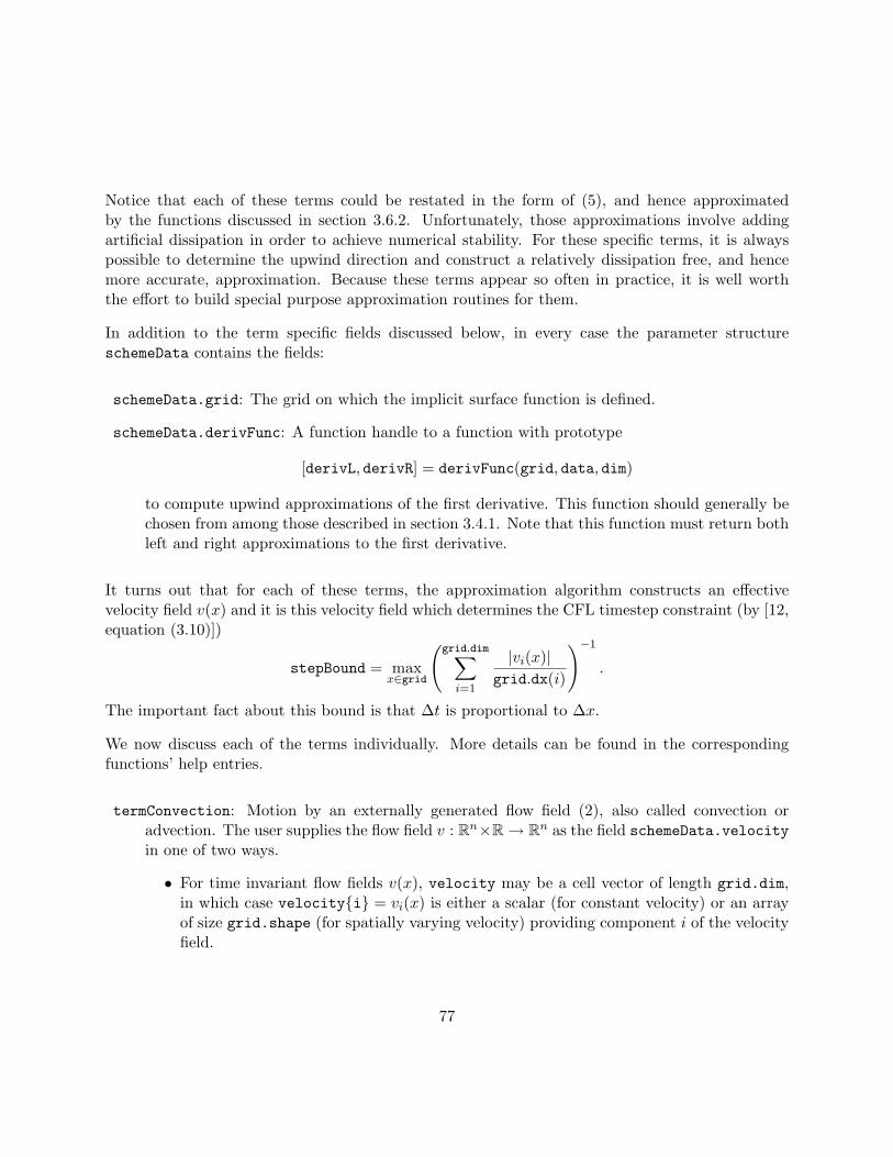
Notice that each of these terms could be restated in the form of (5), and hence approximatedby the functions discussed in section 3.6.2. Unfortunately, those approximations involve addingartificial dissipation in order to achieve numerical stability. For these specific terms, it is alwayspossible to determine the upwind direction and construct a relatively dissipation free, and hencemore accurate, approximation. Because these terms appear so often in practice, it is well worththe effort to build special purpose approximation routines for them.

In addition to the term specific fields discussed below, in every case the parameter structureschemeData contains the fields:

schemeData.grid: The grid on which the implicit surface function is defined.

schemeData.derivFunc: A function handle to a function with prototype

[derivL, derivR] = derivFunc(grid, data, dim)

to compute upwind approximations of the first derivative. This function should generally bechosen from among those described in section 3.4.1. Note that this function must return bothleft and right approximations to the first derivative.

It turns out that for each of these terms, the approximation algorithm constructs an effectivevelocity field v(x) and it is this velocity field which determines the CFL timestep constraint (by [12,equation (3.10)])

stepBound = maxx∈grid

(grid.dim∑

i=1

|vi(x)|grid.dx(i)

)−1

.

The important fact about this bound is that ∆t is proportional to ∆x.

We now discuss each of the terms individually. More details can be found in the correspondingfunctions’ help entries.

termConvection: Motion by an externally generated flow field (2), also called convection oradvection. The user supplies the flow field v : Rn×R → Rn as the field schemeData.velocityin one of two ways.

• For time invariant flow fields v(x), velocity may be a cell vector of length grid.dim,in which case velocity{i} = vi(x) is either a scalar (for constant velocity) or an arrayof size grid.shape (for spatially varying velocity) providing component i of the velocityfield.

77

• For general flow fields, velocity may be a function handle to a function with prototype

v = velocityFunc(t, data, schemeData),

where the output v is the cell vector described above and the input arguments are thesame as those of termConvection (except that data = y has been reshaped to its originalsize). The velocityFunc prototype is very similar to the scalarGridFunc prototype,except that it returns a cell vector of arrays. In a similar way to scalarGridFunc, itmay be useful to include additional fields in schemeData.

termNormal: Motion in the normal direction (3). The user supplies the speed of the interfacea : Rn × R → R as the field schemeData.speed in one of two ways.

• For time invariant speeds a(x), speed may be either a scalar (for constant speed) or anarray of size grid.shape (for spatially varying speed).

• For general speed functions, speed may be a function handle to a function with thescalarGridFunc prototype. The result of evaluating this function at the current timeand state will be treated as the scalar/array described above. In this case, it may beuseful to include additional fields in schemeData.

termReinit: The reinitialization equation (4). In theory, solving this equation to convergence canturn an implicit surface function into a signed distance function without moving or explicitfinding the interface. In practice, it is usually used to smooth out excessively steep or shallowgradients in φ. The user supplies a copy of the initial conditions φ(x, 0) (as an array of sizegrid.shape) in schemeData.initial. This term will rarely be invoked directly, but will beused indirectly by other routines like signedDistanceIterative (see section 3.7.3).

3.6.2 Approximating General HJ Terms

This section discusses the function Kernel/ExplicitIntegration/Term/termLaxFriedrichs andfunctions found in Kernel/ExplicitIntegration/Dissipation.

Terms involving the first derivative in general form (5) are the most challenging to treat numerically,and hence require the most complex term approximation function termLaxFriedrichs. This func-tion is based on the framework proposed in [14] and described in [12, chapter 5.3]. The basic ideais to replace the analytic H(x, p) (where p is a placeholder for ∇φ) with a numerical approximation

H(x, p+, p−) = H

(x,p+ + p−

2

)− α(x)T

[p+ − p−

2

], (25)

where p+ and p− are the right and left approximations of the gradient respectively. The firstterm of H is simply the analytic Hamiltonian evaluated with a centered approximation to the

78

gradient. By itself, such an approximation will be numerically unstable, so the second term addssome dissipation. The final part of this second term (the difference between p+ and p−) looks likea Laplacian, and provides the stabilizing dissipation. In smooth regions of the solution, the leftand right approximations will be similar and this term will be near zero. The scaling portion α(x)of this term depends on DpH(x, p), the partial derivative of H with respect to the gradient p. Asdiscussed below, there are several different choices of α function.

The schemeData structure for termLaxFriedrichs requires the following fields:

schemeData.grid: The grid on which the implicit surface function is defined.

schemeData.derivFunc: A function handle to compute upwind approximations of the first deriva-tive, chosen from among those described in section 3.4.1. Note that this function must returnboth left and right approximations to the first derivative.

schemeData.dissFunc: A function handle to one of the dissipation routines with prototype

[diss, stepBound] = dissFunc(t, data, derivL, derivR, schemeData),

discussed below. Computes the artificial dissipation necessary to stabilize the Hamiltonianapproximation calculated with a centered difference approximation of the gradient; in otherwords, the second term on the right hand side of (25), including the α(x) scaling (which isactually computed by a call to schemeData.partialFunc as described below).

schemeData.hamFunc: A function handle to a routine that computes the analytic H(x, p). Thisfunction is user supplied, and is called directly by termLaxFriedrichs.

schemeData.partialFunc: A function handle to a routine that computes the extrema (in eachdimension) of DpH(x, p). This function is user supplied and is called by dissFunc.

Typically the user will have a mathematical equation for schemeData.hamFunc and simply needsto convert it into (vectorized) Matlab code. Writing schemeData.partialFunc is often morechallenging. The function prototypes are:

hamValue = hamFunc(t, data, deriv, schemeData): Compute the analytic HamiltonianH(x,∇φ);in fact, the more general form H(x, t, φ,∇φ) is allowed. The parameters are the current timet (a scalar), the current implicit surface function φ = data (in an array of size grid.shape),a cell vector ∇φ = deriv of length grid.dim whose element i is an array of size grid.shapecontaining the ith component of the gradient, and the schemeData structure that was passedto termLaxFriedrichs. The return value hamValue should be an array of size grid.shape.

79

alpha = partialFunc(t, data, derivMin, derivMax, schemeData, dim): Estimate compo-nent dim of the α scaling term in (25).

αdim(x) = maxp∈[derivMin,derivMax]

∣∣∣∣∂H(x, p)∂pdim

∣∣∣∣ . (26)

Note that α depends on x, and so should be evaluated separately at each state (preferably ina vectorized fashion). The gradient range parameters derivMin and derivMax are each cellvectors of length grid.dim whose element i is either a scalar or an array of size grid.shape,depending on whether the range of component i of the gradient is constant (for global Lax-Friedrichs) or state dependent (for other types of dissipation). Because the gradient rangemay depend on the dimension, this function is called once for each dimension dim from 1 togrid.dim.

In general, α need not be calculated exactly. Too little dissipation will usually lead to instability,but may be tolerable on the occasional timestep. Too much dissipation will smooth what shouldbe sharp corners in the implicit surface, but is otherwise safe. If the exact optimization in (26)is too complicated or expensive to evaluate, it is reasonable (although somewhat less accurate) tooverestimate its value.

There are a number of options for schemeData.dissFunc provided by the toolbox. They all havethe same prototype

[ diss, stepBound ] = artificialDissipationGLF(t, data, derivL, derivR, schemeData):Compute the artificial dissipation in (25). Parameters derivL = p− and derivR = p+ are thegradient approximations returned by a call to schemeData.derivFunc. The returned diss isan array of size grid.data containing the appropriate dissipation for each node in the grid.The scalar CFL timestep constraint stepBound is also calculated in the dissipation function.

Apart from calculating the difference between the left and right approximations of the gradient,the dissipation routines’ main task is to determine the range of gradient derivMin to derivMaxpass on to schemeFunc.partialFunc. The method of calculating this range differs between thedissipation function options, following the framework laid out in [14, 12].

artificialDissipationGLF: Global Lax-Friedrichs (GLF) dissipation. Calculate a single rangeof gradient over the entire grid, as proposed in the original numerical scheme for finding theviscosity solution of an HJ PDE [3]. Because this choice generates the largest range of possiblegradients, it will also generate the most dissipation.

80

artificialDissipationLLF: Local Lax-Friedrichs (LLF) dissipation. When considering compo-nent αi(x) of the dissipation scaling α(x), restrict the range of component i of the gradientto the range between left and right approximations of that component at each node individ-ually. The range of the remaining components of the gradient is calculated globally, as withGLF. This restriction is more costly to compute, but can be considerably less dissipative forHamiltonians that are very close to convective flow.

artificialDissipationLLLF: Local Local Lax-Friedrichs (LLLF) dissipation. The range of everycomponent of the gradient is simply the range between left and right approximations of thatcomponent at each node individually. This choice leads to the least dissipation and is lessexpensive to compute than LLF (since the same range is used for every dimension). It isequivalent to LLF if the Hamiltonian is separable

H(x, p) =grid.dim∑

i=1

Hi(x, pi).

Unfortunately, in those cases where it is not equivalent to LLF, it can be unstable and/ornonmonotonic. Consequently, any approximation it produces may not converge to the trueviscosity solution as the grid is refined.

Regardless of which dissipation function is chosen, the user supplied schemeFunc.partialFuncwill be called grid.dim times to compute the components of α(x). Furthermore, even if H isindependent of x and GLF is used (so that α(x) is independent of state), the actually dissipationmay be state dependent if the left and right approximations of the gradient vary across the grid.

In addition to scaling the dissipation, α(x) is also the effective velocity and is therefore used tocompute the CFL timestep restriction.

stepBound = maxx∈grid

(grid.dim∑

i=1

|αi(x)|grid.dx(i)

)−1

.

Once again, ∆t is proportional to ∆x. Its effect on the choice of CFL restriction reemphasizesthe fact that overapproximating α is safe (although it will lead to smaller timesteps) but regularunderapproximation may lead to instability.

Two other approximation schemes for arbitrary Hamiltonians are described in [14, 12]: Roe withentropy fix (RF) and Godunov. The former uses upwinding when an upwind direction can bedetermined and some form of Lax-Friedrichs otherwise; thus it will introduce even less dissipationthat the LF schemes discussed above. The latter is less dissipative still, but requires solution of apotentially nonconvex optimization at each node. It seems likely that RF could be implementedin the current toolbox framework for general Hamiltonians, but the same is not true for Godunov;however, the approximation schemes in section 3.6.1 are examples of Godunov solvers for specifictypes of spatial terms.

81

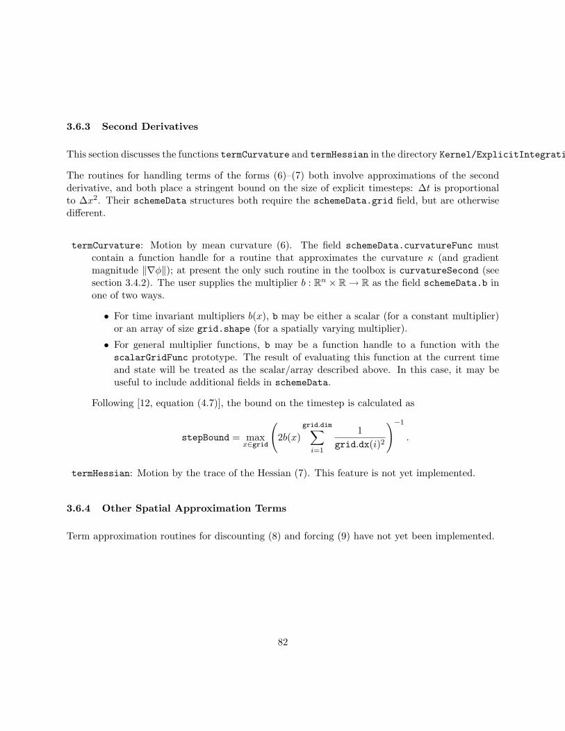
3.6.3 Second Derivatives

This section discusses the functions termCurvature and termHessian in the directory Kernel/ExplicitIntegration/Term/.

The routines for handling terms of the forms (6)–(7) both involve approximations of the secondderivative, and both place a stringent bound on the size of explicit timesteps: ∆t is proportionalto ∆x2. Their schemeData structures both require the schemeData.grid field, but are otherwisedifferent.

termCurvature: Motion by mean curvature (6). The field schemeData.curvatureFunc mustcontain a function handle for a routine that approximates the curvature κ (and gradientmagnitude ‖∇φ‖); at present the only such routine in the toolbox is curvatureSecond (seesection 3.4.2). The user supplies the multiplier b : Rn × R → R as the field schemeData.b inone of two ways.

• For time invariant multipliers b(x), b may be either a scalar (for a constant multiplier)or an array of size grid.shape (for a spatially varying multiplier).

• For general multiplier functions, b may be a function handle to a function with thescalarGridFunc prototype. The result of evaluating this function at the current timeand state will be treated as the scalar/array described above. In this case, it may beuseful to include additional fields in schemeData.

Following [12, equation (4.7)], the bound on the timestep is calculated as

stepBound = maxx∈grid

(2b(x)

grid.dim∑i=1

1grid.dx(i)2

)−1

.

termHessian: Motion by the trace of the Hessian (7). This feature is not yet implemented.

3.6.4 Other Spatial Approximation Terms

Term approximation routines for discounting (8) and forcing (9) have not yet been implemented.

82

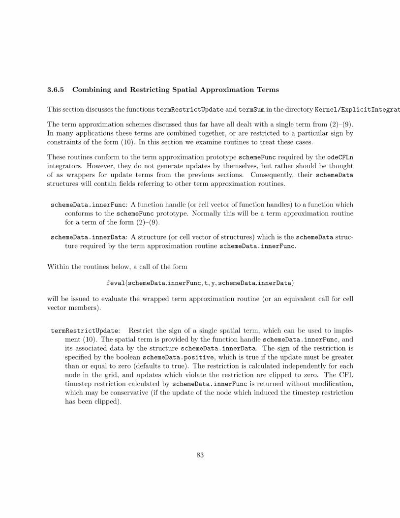
3.6.5 Combining and Restricting Spatial Approximation Terms

This section discusses the functions termRestrictUpdate and termSum in the directory Kernel/ExplicitIntegration/Term/.

The term approximation schemes discussed thus far have all dealt with a single term from (2)–(9).In many applications these terms are combined together, or are restricted to a particular sign byconstraints of the form (10). In this section we examine routines to treat these cases.

These routines conform to the term approximation prototype schemeFunc required by the odeCFLnintegrators. However, they do not generate updates by themselves, but rather should be thoughtof as wrappers for update terms from the previous sections. Consequently, their schemeDatastructures will contain fields referring to other term approximation routines.

schemeData.innerFunc: A function handle (or cell vector of function handles) to a function whichconforms to the schemeFunc prototype. Normally this will be a term approximation routinefor a term of the form (2)–(9).

schemeData.innerData: A structure (or cell vector of structures) which is the schemeData struc-ture required by the term approximation routine schemeData.innerFunc.

Within the routines below, a call of the form

feval(schemeData.innerFunc, t, y, schemeData.innerData)

will be issued to evaluate the wrapped term approximation routine (or an equivalent call for cellvector members).

termRestrictUpdate: Restrict the sign of a single spatial term, which can be used to imple-ment (10). The spatial term is provided by the function handle schemeData.innerFunc, andits associated data by the structure schemeData.innerData. The sign of the restriction isspecified by the boolean schemeData.positive, which is true if the update must be greaterthan or equal to zero (defaults to true). The restriction is calculated independently for eachnode in the grid, and updates which violate the restriction are clipped to zero. The CFLtimestep restriction calculated by schemeData.innerFunc is returned without modification,which may be conservative (if the update of the node which induced the timestep restrictionhas been clipped).

83

termSum: Combine multiple terms by summation. Each of the terms is specified by an entryin the cell vector of function handles schemeData.innerFunc, and its associated data bythe corresponding entry in the cell vector of structures schemeData.innerData. Each termis evaluated independently, and the updates are summed at each node. The overall CFLtimestep restriction stepBoundsum is computed from the individual term’s timestep restrictionsstepBoundi by:

stepBoundsum =

(∑i

1stepBoundi

)−1

.

Note that termRestrictUpdate and termSum can be used to wrap each other, and thereby accom-plish HJ PDEs more complex than (1)–(10). They could even be used to wrap themselves, althoughwe can think of little benefit to be gained from that design.

3.7 Helper Routines

This section describes functions in Examples/Helper, which are used for various auxiliary tasks.

3.7.1 Error Checking

This section describes functions in Examples/Helper/ErrorCheck, which are used to check thevalidity of function arguments.

checkStructureFields(structure, ’field1’, ’field2’, ...): Checks that the first argu-ment structure is a structure and, if so, checks that the subsequent arguments (whichshould all be strings) are the names of fields in that structure. Causes an error if either checkfails. Often used in functions which access the schemeData structure.

84

3.7.2 Math

This section describes functions in Examples/Helper/Math, which are various types of mathemat-ical operations.

The first is an example of the postTimestepFunc protocol and implements its most common ap-plication, the masking or constraint of φ (11).

[ yOut, schemeDataOut ] = postTimestepMask(t, yIn, schemeDataIn): Constrains the valueof φ(x, t) after each timestep by applying a binary mask operation. The input argument t isignored, while the input array yIn provides the value of φ(x, t). The structure schemeDataInmust contain the fields maskFunc and maskData. The output argument schemeDataOut =schemeDataIn (no change), while the modified data array yOut is calculated by

yOut = feval(schemeDataIn.maskFunc, yIn, schemeDataIn.maskData).

A typical application of postTimestepMask would be to enforce the constraint φ(x, t) ≥ ψ(x).This constraint can be implemented by choosing maskFunc = @max and maskData to be an arrayrepresenting ψ(x), reshaped into a column vector.

The remaining functions in this directory implement an extended form of some simple matrixoperations. In several parts of the toolbox, it is necessary to represent spatially varying matricesA(x) or vectors v(x)—in fact, x itself is a spatially varying vector. These objects are a challengeto represent, since the toolbox has already adopted the convention that Matlab’s array indicesrefer to nodes in the spatial grid. Adding more indices to account for the entries in the spatiallyvarying matrix or vector would lead to a great deal of index confusion.

As an alternative, we have chosen to represent such matrices and vectors as cell arrays. A matrixA(x) ∈ Rp×q, where x ∈ Rn is represented by a two dimensional cell array with p rows and qcolumns. Each element of this cell array is a regular Matlab array of dimension n, containingelements for every node x in the computational grid. We call this object a cell matrix. For example,the field grid.xs in the grid structure can be thought of as a n× 1 cell matrix description of thevector x.

Several operations are provided for cell matrices:

addition: A(x) + B(x),multiplication: A(x)B(x),

elementwise maximization: maxx

A(x) or maxx|A(x)|.

85

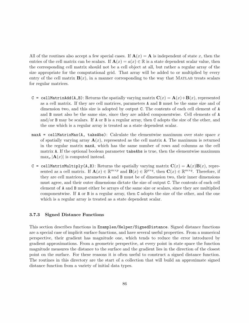
All of the routines also accept a few special cases. If A(x) = A is independent of state x, then theentries of the cell matrix can be scalars. If A(x) = a(x) ∈ R is a state dependent scalar value, thenthe corresponding cell matrix should not be a cell object at all, but rather a regular array of thesize appropriate for the computational grid. That array will be added to or multiplied by everyentry of the cell matrix B(x), in a manner corresponding to the way that Matlab treats scalarsfor regular matrices.

C = cellMatrixAdd(A,B): Returns the spatially varying matrix C(x) = A(x)+B(x), representedas a cell matrix. If they are cell matrices, parameters A and B must be the same size and ofdimension two, and this size is adopted by output C. The contents of each cell element of Aand B must also be the same size, since they are added componentwise. Cell elements of Aand/or B may be scalars. If A or B is a regular array, then C adopts the size of the other, andthe one which is a regular array is treated as a state dependent scalar.

maxA = cellMatrixMax(A, takeAbs): Calculate the elementwise maximum over state space xof spatially varying array A(x), represented as the cell matrix A. The maximum is returnedin the regular matrix maxA, which has the same number of rows and columns as the cellmatrix A. If the optional boolean parameter takeAbs is true, then the elementwise maximummaxx |A(x)| is computed instead.

C = cellMatrixMultiply(A,B): Returns the spatially varying matrix C(x) = A(x)B(x), repre-sented as a cell matrix. If A(x) ∈ Rm×p and B(x) ∈ Rp×q, then C(x) ∈ Rm×q. Therefore, ifthey are cell matrices, parameters A and B must be of dimension two, their inner dimensionsmust agree, and their outer dimensions dictate the size of output C. The contents of each cellelement of A and B must either be arrays of the same size or scalars, since they are multipliedcomponentwise. If A or B is a regular array, then C adopts the size of the other, and the onewhich is a regular array is treated as a state dependent scalar.

3.7.3 Signed Distance Functions

This section describes functions in Examples/Helper/SignedDistance. Signed distance functionsare a special case of implicit surface functions, and have several useful properties. From a numericalperspective, their gradient has magnitude one, which tends to reduce the error introduced bygradient approximations. From a geometric perspective, at every point in state space the functionmagnitude measures the distance to the surface and the gradient lies in the direction of the closestpoint on the surface. For these reasons it is often useful to construct a signed distance function.The routines in this directory are the start of a collection that will build an approximate signeddistance function from a variety of initial data types.

86

data = signedDistanceIterative(grid, data0, tMax, errorMax, accuracy): Turns an im-plicit surface function into a signed distance function by iterative solution of the reinitializa-tion PDE (4). Both the implicit surface function and signed distance functions are defined onthe same computational grid, the parameter grid. The implicit surface function is given byinput array data0, and the signed distance result by output array data. The optional param-eter tMax implicitly defines how many iterations to make, and defaults to a value high enoughthat the reinitialization front will have reached across the entire grid. The optional parametererrorMax defines an update magnitude tolerance relative to the longest grid cell edge lengthmax(grid.dx)—if the average node update drops below this tolerance on any iteration, thereinitialization is assumed to have converged and the iterations are terminated. The defaultvalue of 1e-3 is so tight that iterations rarely converge under the default. The optional pa-rameter accuracy has the usual options determining what order of accuracy of spatial andtemporal derivative approximations should be used for the reinitialization PDE, and defaultsto ’medium’ (second order accurate). Note that the input implicit surface function must berelatively well behaved for this operation to succeed: the function gradient should not changesign or direction too drastically between neighboring nodes near the implicit surface. Even forwell behaved implicit surface functions, this operation may shift the implicit surface locationslightly.

data = unsignedDistanceFromPoints(grid, points): Creates a function whose value at eachgrid node measures the distance from that grid node to the nearest of a collection of points.The grid is defined by parameter grid and each point is a row (with grid.dim columns) of theparameter points. The unsigned distance function is returned in array data. The unsigneddistance function is not an implicit surface function. Searching for the zero level set willprove futile, since all node values will be non-negative. In fact, this routine is simply the firststep in turning a collection of surface points into an implicit surface function (for example,see [12, chapter 13]). Furthermore, this implementation uses the brute force, quadratic timepairwise algorithm. In future versions it should be replaced by a much quicker fast marchingalgorithm for unsigned distance [15].

3.7.4 Visualization

This section describes functions in Examples/Helper/Visualization, which are used to simplifyvarious visualization tasks.

h = addSlopes(point, width, styles, slopes, labels): Plots one or more lines of specifiedslope. When plotting experimental convergence rates of algorithms, it is often useful to havecomparison lines of specified slope, which correspond to certain theoretical convergence rates.This function is usually called for a figure which has already been created (and hopefully has

87

hold on so that addSlopes does not destroy the existing figure). For example, the scriptfirstDerivSpatialConverge in section 2.7.2 uses addSlopes when creating figure 22. Vectorparameter point (with two elements) specifies a point from which all slope lines emanate tothe right. Scalar parameter width specifies the extent of the lines in the horizontal direction.Parameter styles may be a string or a cell vector of strings, which specifies the line style(s)of the slope lines. Vector parameter slopes is a list of slope lines which should be shown.Cell vector parameter labels contains one string for each slope line, which is displayed to theright of the end point of the corresponding slope line. The output h is a two column array ofgraphic handles; the first column contains the line handles for the slope lines and the secondcolumn the text handles for the labels.

spinAnimation(fig, filename, compress): A routine which demonstrates how to use Mat-lab’s animation facilities to generate an animation of a spinning three dimensional plot.When working with surfaces in three dimensions, it is often difficult to understand the shapewithout seeing it from several angles. Interactive Matlab has rotate3d, but it is difficultto use during a talk; consequently it is usually better to generate an animation showing thesurface from many different angles—if you have seen the author of the toolbox give a talk,then you have probably seen an animation created by this routine. The parameter fig is afigure handle to the already created three dimensional plot. The string parameter filenameis the name of the output animation file (which will have the extension .avi appended).The boolean parameter compress specifies whether lossy compression should be used to (sig-nificantly) reduce the size of the resulting animation, at the expense of some image quality.Remaining parameters, such as animation resolution, number of frames and compression qual-ity, can be set within the source code. Note that this function will probably work only in theWindows environment, since it uses the avi file format.

h = visualizeLevelSet(g, data, displayType, level, titleStr): Create a visualizationof an implicit surface function. At present, dimensions one to three are supported. This func-tion is designed to produce quick visualizations of implicit surface functions, rather than pol-ished figures. While many of the figures in this document started as calls to visualizeLevelSet,they were usually then modified by adding labels, improving the viewing angle and/or light-ing, or adding more graphical objects. The visualization is created within the current figureand axis, so this function can be used with subplot and to create multiple implicit surfacesin a single plot. The grid structure is given by parameter g, and the implicit surface functionby array parameter data. The string parameter displayType specifies which type of visu-alization to use; the options depend on the dimension of the grid and are given in the helpentry for this routine. The optional scalar level specifies which level set to visualize, anddefaults to zero. The optional string titleStr creates a title text object for the current axis.

88

4 Future Features

At the completion of this version of the toolbox, among the extensions which seem useful are:

• Implementation of term approximation routines for motion by the trace of the Hessian (7),discounting (8) and forcing (9).

• More general Dirichlet and Neumann boundary conditions.

• The WENO3 upwind first order spatial derivative scheme.

• Roe-Fix and possibly Gudonov numerical Hamiltonians. Stencil Lax-Friedrichs artificial dis-sipation.

• ENO/WENO function value interpolation (not just gradients) away from nodes.

• Implicit time stepping (with Matlab’s ODE suite?).

• Some method to avoid constant reallocation of memory for ghost cells.

• Adaptively refined grids.

• Construction of signed distance functions from point clouds.

• Examples from various application fields.

Do you have any other ideas?

Acknowledgements: The author would like to thank Ronald Fedkiw and Stanley Osher for ex-tensive discussions about the details of numerical schemes for solving the Hamilton-Jacobi PDE.Additional discussions with Jean-Pierre Aubin, David Adalsteinsson, Alexandre Bayen, Doug En-right, L. C. Evans, Chiu-Yen Kao, Alexander Kurzhanski, Doron Levy, John Lygeros, JianliangQian, Patrick Saint-Pierre, Jamie Sethian, Steven Ruuth, Pravin Varaiya, Alexander Vladimirsky,Hong-Kai Zhao and many others have contributed to my understanding of the field. Without thesupport of Claire Tomlin and Shankar Sastry this toolbox would not have been possible. Devel-opment and release of the code and documentation for this version is supported by the NationalScience and Engineering Research Council of Canada and the Department of Computer Science atthe University of British Columbia.

89

References

[1] M. Bardi and I. Capuzzo-Dolcetta. Optimal Control and Viscosity Solutions of Hamilton-Jacobi-Bellman equations. Birkhauser, Boston, 1997.

[2] P. Cardaliaguet, M. Quincampoix, and P. Saint-Pierre. Set-valued numerical analysis for op-timal control and differential games. In M. Bardi, T. E. S. Raghavan, and T. Parthasarathy,editors, Stochastic and Differential Games: Theory and Numerical Methods, volume 4 of An-nals of International Society of Dynamic Games, pages 177–247. Birkhauser, 1999.

[3] M. G. Crandall and P.-L. Lions. Two approximations of solutions of Hamilton-Jacobi equations.Mathematics of Computation, 43(167):1–19, 1984.

[4] L. C. Evans. Partial Differential Equations. American Mathematical Society, Providence,Rhode Island, 1998.

[5] R. Fedkiw, T. Aslam, B. Merriman, and S. Osher. A non-oscillatory Eulerian approach tointerfaces in multimaterial flows (the ghost fluid method). Journal of Computational Physics,152:457–492, 1999.

[6] Peter E. Kloeden and Eckhard Platen. Numerical Solution of Stochastic Differential Equations.Applications of Mathematics. Springer, third edition, 1999.

[7] I. Mitchell, A. Bayen, and C. J. Tomlin. Computing reachable sets for continuous dynamicgames using level set methods. Submitted January 2004 to IEEE Transactions on AutomaticControl.

[8] I. Mitchell and C. Tomlin. Level set methods for computation in hybrid systems. In B. Kroghand N. Lynch, editors, Hybrid Systems: Computation and Control, number 1790 in LectureNotes in Computer Science, pages 310–323. Springer Verlag, 2000.

[9] Ian M. Mitchell. Application of Level Set Methods to Control and Reachability Problems inContinuous and Hybrid Systems. PhD thesis, Scientific Computing and Computational Math-ematics Program, Stanford University, August 2002.

[10] Bernt Øksendal. Stochastic Differential Equations: an Introduction with Applications.Springer, sixth edition, 2003.

[11] S. Osher. A level set formulation for the solution of the Dirichlet problem for Hamilton-Jacobiequations. SIAM Journal of Mathematical Analysis, 24(?):1145–1152, 1993.

[12] S. Osher and R. Fedkiw. Level Set Methods and Dynamic Implicit Surfaces. Springer-Verlag,2002.

90

[13] S. Osher and J. A. Sethian. Fronts propagating with curvature-dependent speed: Algorithmsbased on Hamilton-Jacobi formulations. Journal of Computational Physics, 79:12–49, 1988.

[14] S. Osher and Chi-Wang Shu. High-order essentially nonoscillatory schemes for Hamilton-Jacobiequations. SIAM Journal on Numerical Analysis, 28(4):907–922, 1991.

[15] J. A. Sethian. Level Set Methods and Fast Marching Methods. Cambridge University Press,New York, 1999.

[16] Chi-Wang Shu and Stanley Osher. Efficient implementation of essentially non-oscillatory shock-capturing schemes. Journal of Computational Physics, 77:439–471, 1988.

[17] C. Tomlin, J. Lygeros, and S. Sastry. A game theoretic approach to controller design for hybridsystems. Proceedings of the IEEE, 88(7):949–970, July 2000.

[18] C. Tomlin, I. Mitchell, A. Bayen, and M. Oishi. Computational techniques for the verificationof hybrid systems. Proceedings of the IEEE, 91(7):986–1001, July 2003.

91

Concept Index

Reading the Index: Roman page numbersindicate discussion of the concept or command.Italic page numbers indicate an example of itsuse.

boundary conditions: 17, 61–62Dirichlet: 61extrapolated: 17, 61, 62Neumann: 61periodic: 17, 61

cell matrix: 85constraints: see term approximation, constraints

constructive solid geometry: see initial condi-tions

convection: see term approximation, convec-tion

curvature: see term approximation, curvature

initial conditions: 54, 63–66basic shapes: 63–65reinitialization: see term approximation,

reinitializationset operations: 65–66

masking: see term approximation, constraints

reachable sets: 42–53continuous: 43–45, 45–50Hamiltonian for: 43, 48, 50HJ PDE for: 43hybrid: 45, 50–53

reinitialization: see term approximation, reini-tialization

set operations: see initial conditions

spatial derivative: 21, 66–71centered: 70, 71convergence rate of: 54–56ENO: 21, 56, 67, 68first: 21, 56, 67, 68, 71second: 70, 71upwind: 21, 56, 66–69WENO: 21, 56, 67

term approximation: 6–8, 75–84advection: see convectioncombining: 35, 84constraints

on φ: 8, 29–31, 53, 75, 85on Dtφ: 8, 43, 83

convection: 7, 12–25, 35, 76, 77curvature, mean: 8, 32–34, 82discount: 8forcing: 8general HJ: 7, 27–28, 43–45, 78–81Hessian, trace of the: 8, 82Lax-Friedrichs: 27–28, 43–45, 78–81

artificial dissipation: 80–81estimating the partials: 28, 41, 42, 45,

48, 50, 80mean curvature: see curvature, meannormal direction: 7, 34–35, 78reinitialization: 7, 25–26, 78, 87velocity field: see convection

time derivative: 7, 21, 71–75PostTimestep option: 8, 30, 75explicit integrator: 21, 72–74TVD RK: 72, 73

92

Command Index

Reading the Index: Roman page numbersindicate discussion of the concept or command.Italic page numbers indicate an example of itsuse.

acoustic: 50acousticHamFunc: 50acousticPartialFunc: 50addGhostAllDims: 62addGhostDirichlet: 61addGhostExtrapolate: 17, 61, 62addGhostNeumann: 61addGhostPeriodic: 17, 61addNodesAllDims: 62addPathToKernel: 12, 15addSlopes: 87air3D: 47air3DHamFunc: 48air3DPartialFunc: 48airMode: 53argumentSemanticsTest: 58artificialDissipationGLF: 28, 40, 42, 80artificialDissipationLLF: 28, 40, 42, 81artificialDissipationLLLF: 28, 40, 42, 81

burgersLF: 40

cellMatrixAdd: 65, 86cellMatrixMax: 86cellMatrixMultiply: 18, 19, 65, 86centeredFirstSecond: 71checkEquivalentApprox: 69checkStructureFields: 25, 84

convectionDemo: 12–25curvatureSecond: 70curvatureSpiralDemo: 32curvatureStarDemo: 33

dumbbell1: 38

figureAir3D: 48findReachSet: 53firstDerivSpatialConverge: 56firstDerivSpatialTest1: 54

ghostCell: 58

hessianSecond: 70

initialConditionsTest1D: 54initialConditionsTest2D: 54initialConditionsTest3D: 54

laplacianSecond: 71laxFriedrichsDemo: 27laxFriedrichsDemoHamFunc: 28laxFriedrichsDemoPartialFunc: 28

maskAndKeepMin: 30maskDemo: 31

nonconvexLF: 42normalStarDemo: 35

odeCFL1: 21, 72odeCFL2: 21, 73odeCFL3: 21, 73odeCFLn: 23, 73

93

odeCFLset: 21, 74

postTimestepMask: 53, 85processGrid: 17, 60prototypes

derivFunc: 21, 77dissFunc: 28, 40, 42, 79, 80hamFunc: 28, 41, 42, 44, 48, 50, 79partialFunc: 28, 41, 42, 44, 48, 50, 80postTimestepFunc: 30, 53, 75, 85scalarGridFunc: 25, 34, 35, 76schemeFunc: 21, 35, 47, 73, 75, 83velocityFunc: 19, 25, 78

reinitDemo: 26reinitTest: 58

shapeComplement: 66shapeCylinder: 64shapeDifference: 66shapeHyperplane: 65shapeIntersection: 65shapeRectangleByCenter: 64shapeRectangleByCorners: 64shapeSphere: 63shapeUnion: 65signedDistanceIterative: 58, 87spinAnimation: 88spinStarDemo: 35spiralFromEllipse: 33spiralFromPoints: 33switchValue: 19, 24–25, 34, 35

termConvection: 21, 30, 35, 52, 76, 77termCurvature: 32, 37, 38, 82termHessian: 82

termLaxFriedrichs: 28, 40, 42, 44, 47, 50,78–81

termNormal: 35, 37, 78termReinit: 26, 78termRestrictUpdate: 43, 47, 50, 52, 83termSum: 35, 37, 84tripleSine: 37

unsignedDistanceFromPoints: 87upwindFirstENO2: 21, 56, 67upwindFirstENO3: 21, 67, 68upwindFirstENO3a: 56, 68upwindFirstENO3aHelper: 69upwindFirstENO3b: 56, 68upwindFirstENO3bHelper: 69upwindFirstFirst: 21, 56, 67upwindFirstWENO5: 21, 67upwindFirstWENO5a: 56, 68upwindFirstWENO5b: 56, 68

visualizeLevelSet: 22, 24, 88

94