1

Smoothed particle hydrodynamics in a generalized coordinate system with a finite-

deformation constitutive model

Shigeki Yashiro a,*, Tomonaga Okabe b

a Department of Mechanical Engineering, Shizuoka University

3-5-1 Johoku, Naka-ku, Hamamatsu 432-8561, Japan

b Department of Aerospace Engineering, Tohoku University

6-6-01, Aoba-yama, Aoba-ku, Sendai 980-8579, Japan

* Corresponding author: Tel: +81-53-478-1026; Fax: +81-53-478-1026.

E-mail address: yashiro.shigeki@shizuoka.ac.jp (S. Yashiro)

Abstract

This study proposes smoothed particle hydrodynamics (SPH) in a generalized coordinate

system. The present approach allocates particles inhomogeneously in the Cartesian coordinate

system, and arranges them via mapping in a generalized coordinate system in which the

particles are aligned at a uniform spacing. This characteristic enables us to employ fine division

only in the direction required, e.g., in the through-thickness direction for a thin-plate problem,

and thus to reduce computation cost. This study provides the formulation of SPH in a

generalized coordinate system with a finite-deformation constitutive model and then verifies it

by analyzing quasi-static and dynamic problems of solids. High-velocity impact test was also

performed with an aluminum target and a steel sphere, and the predicted crater shape agreed

well with the experiment. Furthermore, the numerical study demonstrated that the present

approach successfully reduced the computation cost with marginal degradation of accuracy.

Keywords: Solids, Particle methods, Impact, Mapping

Accep

ted

Man

uscr

ipt

2

1. Introduction

Meshless methods will overcome difficulties associated with reliance on a mesh to construct

the approximation when analyzing moving discontinuities. One of the first meshless methods

is smooth particle hydrodynamics (SPH) developed by Gingold and Monaghan [1] and Lucy

[2]. Another most popular meshless methods are the element-free Galerkin (EFG) method [3],

the reproducing kernel particle method (RKPM) [4], and the meshless local Petrov-Galerkin

(MLPG) method [5]. A number of different meshless methods [6-12] have been developed in

recent years, and a good review on meshless methods and their implementation can be found

in literature, e.g., [13].

Among them, SPH has been improved and been applied to engineering problems by many

researchers. This method was first developed to predict astrophysical phenomena with

compressible flow [1,2], and has been applied to incompressible flow [14], viscous flow [15-

18], and solids [19-23]. A coupled analysis between fluid and structure has also been performed

[24,25]. In recent years, SPH has been used in a wide range of engineering fields including

high- and hyper-velocity impact in armor systems [26] and space debris shields [27,28],

machining [29], die casting and forging of metals [30,31], dam spillway flow [32], and

geophysical problems of magma chambers [33] and lava flow [34]. Recent reviews of SPH can

be found in the literature [35,36].

In standard SPH, particles initially have to be aligned at uniform intervals in the Cartesian

coordinate system. Specifically, when analyzing thin-plate problems, fine division is necessary

in the through-thickness direction to achieve sufficient accuracy. However, close particle

spacing drastically increases the calculation cost due to the increase in the total number of

particles. The particle spacing can be altered in part of an analytical model (but still be uniform)

Accep

ted

Man

uscr

ipt

3

[24,28]. This method will be useful in problems where stresses change steeply only in a limited

region of the model. However, fine particles must be used over the whole model if a steep stress

gradient is possible throughout the model.

In recent years, a number of researchers have investigated accuracy improvement of SPH.

Wong and Shie [37] developed a Galerkin-based SPH formulation with moving least-squares

approximation in combination with updated Lagrangian kernel functions to remove instabilities.

They applied it to impact problems with large deformation. Herreros and Mabssout [38]

proposed Taylor-SPH with a two-step time-discretization scheme and demonstrated its accuracy

by predicting shock-wave propagation. Blanc and Pastor [39] extended the algorithm using a

Runge-Kutta integration scheme to improve the accuracy and stability for large deformation

problems. Colagrossi et al. [40] proposed a particle-packing algorithm to reduce numerical

noise due to particle resettlement during the early stages of the flow evolution. Vacondio et al.

[41] proposed a variable resolution scheme that dynamically modified particle sizes by splitting

and merging individual particles to provide good resolution. Puri and Ramachandran [42]

compared the accuracy and robustness between the current state-of-the-art SPH schemes,

namely standard SPH with an adaptive density kernel estimation technique, the variational SPH

formulation, and the Godunov-type SPH scheme, for compressible Euler equations.

However, few studies seek to reduce computation costs. Maurel and Combescure [43]

introduced Mindlin-Reissner’s thick shell theory into SPH to reduce computation cost for

analyzing thin structures. A thin plate is modeled by a single layer of particles having three

degrees of freedom in translation and two degrees of freedom in rotation. They successfully

applied it to impact fracture. Furthermore, Combescure and colleagues [44] extended the SPH

shells to represent dynamic fracture with sharp discontinuities.

Fine particles will be used for analyzing extension of microscopic damage in materials such

Accep

ted

Man

uscr

ipt

4

as composite laminates [45], but in some cases, fine division will be required only in the

through-thickness direction. This study therefore proposes SPH in a generalized coordinate

system to achieve inhomogeneous particle placement. More specifically, we allocate particles

inhomogeneously in the Cartesian coordinate system, and then arrange them at a uniform

interval in a generalized coordinate system via mapping. The conservation equations, as well

as the updates in the particle positions, are solved in the mapped space by using the standard

scheme of SPH. This enables us to obtain fine division only in the direction required, e.g., in

the through-thickness direction for a thin-plate problem. This method can be a breakthrough

improving the computational efficiency of SPH by reducing the total number of particles.

This paper is organized as follows. Section 2 provides the formulation of SPH in a

generalized coordinate system with a finite-deformation constitutive model. In Section 3, the

newly developed SPH is applied to quasi-static bending problem of a thin plate for verification.

Accuracy of the bending results is compared between the present approach and the standard

method to demonstrate the advantage of the use of a generalized coordinate system. Finally,

Section 4 presents the experiment and analysis of high-velocity impact of a steel sphere on an

aluminum plate. We will discuss validity and usefulness of SPH in a generalized coordinate

system.

2. Theory

2.1 Generalized coordinate system

Consider the origin O, the regular Cartesian coordinate system (x1, x2, x3), and a generalized

coordinate system (θ1, θ2, θ3). Coordinates θ1, θ2, and θ3 are equal to coordinates x1, x2, and x3

multiplied by 1/a, 1/b, and 1/c. Here, a variable with a superscript (subscript) denotes a

contravariant (covariant) component of a tensor. An arbitrary vector R is represented by

Accep

ted

Man

uscr

ipt

5

ii

iix geR , where ei and gi (i = 1, 2, 3) are the orthonormal base unit vector and the

covariant base vector. The covariant base vector is calculated by

ji

j

ii

xe

Rg

. (1)

Equation (1) provides the relations of g1 = ae1, g2 = be2, and g3 = ce3 for the coordinate system

considered. The contravariant base vector gi is given by

jj

ii

xeg

. (2)

The following relations are derived between the covariant base vector and the contravariant

base vector based on a generalized tensorial analysis.

ijji ggg (3)

ijji ggg (4)

ji

ji gg (5)

jiji g gg (6)

jiji g gg (7)

gij (gij) is the covariant (contravariant) metric tensor, and ji is the unit tensor. These equations

transform the covariant component into the contravariant component (and vice versa) for a

vector v.

hihi vgv and h

ihi vgv (8)

Now, let us define parameters ih~

and g that relate the components of an arbitrary tensor in

the physical space to those in the mathematical space.

ii

ig

h1~

(no sum on i) (9)

222 cbagg ij (10)

A component of a vector iiv ev ~ in the physical space is transformed into one in the

considered mathematical space as follows.

Accep

ted

Man

uscr

ipt

6

iii vhv

~~ and i

ii

h

vv ~~ (no sum on i) (11)

This equation will be used when presenting field variables in the physical space.

2.2 Governing equations

The governing equations for continuum mechanics express the conservation of mass and

momentum, and these equations are solved in the updated Lagrangian scheme. The

conservation equation of mass is

i

ivg

gt 1

d

d, (12)

where ρ is the density, t is the time, and vi is the velocity. Since g is constant for the base vector

in this study, Eq. (12) is simplified to

i

iv

t

d

d. (13)

The conservation equation of momentum is, at the current configuration,

j

jii

t

v 1

d

d , (14)

where σij is the first Piola-Kirchhoff stress tensor, and □|i denotes the covariant derivative. Note

that the Christoffel symbol is zero in the coordinate system considered, and the covariant

derivative □|i is then simplified to □,i = ∂□/∂θi.

2.3 Constitutive equations

This section presents a finite-deformation constitutive model. A classical elastic-plastic

theory was used, and the following rate-form potential was considered.

klijijklep DDCU

2

1~ (15)

Accep

ted

Man

uscr

ipt

7

lkjiijklepep C ggggC is the elastic-plastic stiffness tensor, and ji

ijD ggD is the

deformation rate tensor. Based on the von Mises plastic potential and the associated flow rule,

the yield function F and basic equations are as follows.

22

3

1 py eF (16)

TT :2

32 (17)

TD p (18)

H

e

e

ep

2

94

::

::

2

3

TCT

DCT (19)

Here, is the equivalent stress, σy is the yield stress, pe is the equivalent plastic strain, T’

is the deviatoric stress tensor, and H’ is the hardening coefficient. The constitutive equation is

peJt t DDCT :ˆ

, (20)

where the left-hand-side is the Jaumann rate of the Kirchhoff stress, C-e is the stiffness tensor

of an isotropic elastic medium, and Dp is the plastic strain rate. Although C-ep in Eq. (15) can

be derived, this study used Eq. (20) for stability of the analysis. The rate of the Cauchy stress

is thus

WTTWTDDCT tJtp

e : , (21)

where tJt is the modulus of volume change, and W is the spin tensor.

After this point, variables in the physical space are indicated with tildes. The stiffness tensor

in mathematical space, ijkleC , is converted from that in the physical space as follows.

lkjiijkle

ijkle hhhhCC

~~~~~ (no sum on i, j, k, and l) (22)

When the stress tensor and strain tensor is calculated in the mathematical space, those in the

physical space can be obtained by

ijjiij hh ~~~ (no sum on i and j), (23)

Accep

ted

Man

uscr

ipt

8

and

ij

ji

ij Thh

T ~1

~1~ (no sum on i and j). (24)

2.4 SPH method

The density ρ in the mathematical space is considered to be equal to that in the physical space,

~ . The mass of a particle in the mathematical space, m, is then defined by

3~

dg

mm , (25)

where d is the uniform particle spacing in the initial condition in the mathematical space.

Equation (25) indicates that m is independent of the scale parameters a, b, and c.

SPH is based on interpolation theory. The method allows a function to be expressed in terms

of its values at a set of disordered points using a kernel function. The kernel function W refers

to a weighting function and specifies the contribution of a field variable x at a certain

position x. The interpolation of x is defined as

D

hW xxxxx d, . (26)

D is the volume considered, and the smoothing length h represents the effective width of the

kernel. The very basic interpolation equation (Eq. (26)) can be evaluated only in mathematical

space, since 3d dm x is independent of the scale. If there are N particles in the effective

width of the kernel function from position x, Eq. (26) is approximated by

N

bb

b

bb hW

m

1

,xxx

, (27)

where b denotes the label of a neighboring particle, and the brackets indicate that the

variable is approximated by the SPH interpolation. A particle equation for the gradient of x

can be obtained by using the divergence theorem of Gauss and the fact that W vanishes at

infinity.

Accep

ted

Man

uscr

ipt

9

N

bb

b

bbD

hWm

hW1

,d, xxxxxxx

(28)

The kernel function should have a symmetric shape that satisfies both the limit condition and

the normalization condition. Compact support kernels are usually used for calculation efficiency.

A cubic B-spline function is used in this study:

otherwise,0

,21for 24

1

,10for 4

3

2

31

, 3

32

0 ss

sss

WhW r (29)

where s = |r|/h; the normalization constant W0 is 10/(7πh2) in a two-dimensional analysis, and

1/(πh3) in a three-dimensional analysis.

The total time derivative (d/dt) is taken in a moving Lagrangian frame, and the transform of

governing equations (13) and (14) into particle equations yields the following set of SPH

equations:

abiab

bi

ai

b

ba

a Wvv

m

t

d

d, (30)

ab

iab

abij

b

bij

a

aij

ba

j Wm

t

v

~

d

d22 , (31)

where subscripts a and b denote the labels of the particle of interest and its neighboring particles.

~ is the artificial viscosity term to stabilize dynamic response and is evaluated in the physical

space. Note that δij is the tensor converted from the unit tensor in the physical space, ij~ , by

the same manner as in Eq. (24). The deformation rate tensor and the spin tensor represented as

i

j

ji

ijjiij

vvvvD

2

1

2

1 (32)

i

j

ji

ijjiij

vvvvW

2

1

2

1 (33)

are discretized by particles in the same manner as with standard SPH.

Accep

ted

Man

uscr

ipt

10

ba

iab

ajbjjab

aibib

baij

Wvv

Wvv

mD

2

1 (34)

ba

iab

ajbjjab

aibib

baij

Wvv

Wvv

mW

2

1 (35)

Since all of the variables are written in mathematical space, the same calculation procedure

as for standard SPH is available for the above formulation paying attention to the “covariant”

(subscript) or “contravariant” (superscript).

2.5 Time integration

The time-step size should be sufficiently small to stably analyze the time integration. Time

step Δt is determined by the Courant-Friedrichs-Levy condition.

v~~

,,minmin

c

cbaht

(36)

ω is 0.3 to ensure that a particle moves only a fraction of the smoothing length h per time-step.

The Runge-Kutta-Gill method was employed as the time-integration scheme.

2.6 Stress boundary condition

For simplicity, the stress boundary condition is expressed by imposing equivalent external

forces on the particles in a surface instead of enforcing tractions on the surface. If a body force

F is given to a particle, the acceleration F/ρ is added to the right-hand-side of Eq. (31) for the

particle concerned based on the conservation of momentum. If a force F is given to a particle,

the corresponding acceleration is first calculated in the physical space.

mt ~d

d Fv (37)

The acceleration is then converted into that in mathematical space by using Eq. (11) and is

added to the acceleration calculated by Eq. (31).

Accep

ted

Man

uscr

ipt

11

3. Verification

Before applying the proposed approach to specific problems, we first confirmed that valid

stresses and strains are predicted for quasi-static uniaxial tension and pure shear. This section

verifies the proposed approach by predicting quasi-static three-point bending in a thin plate.

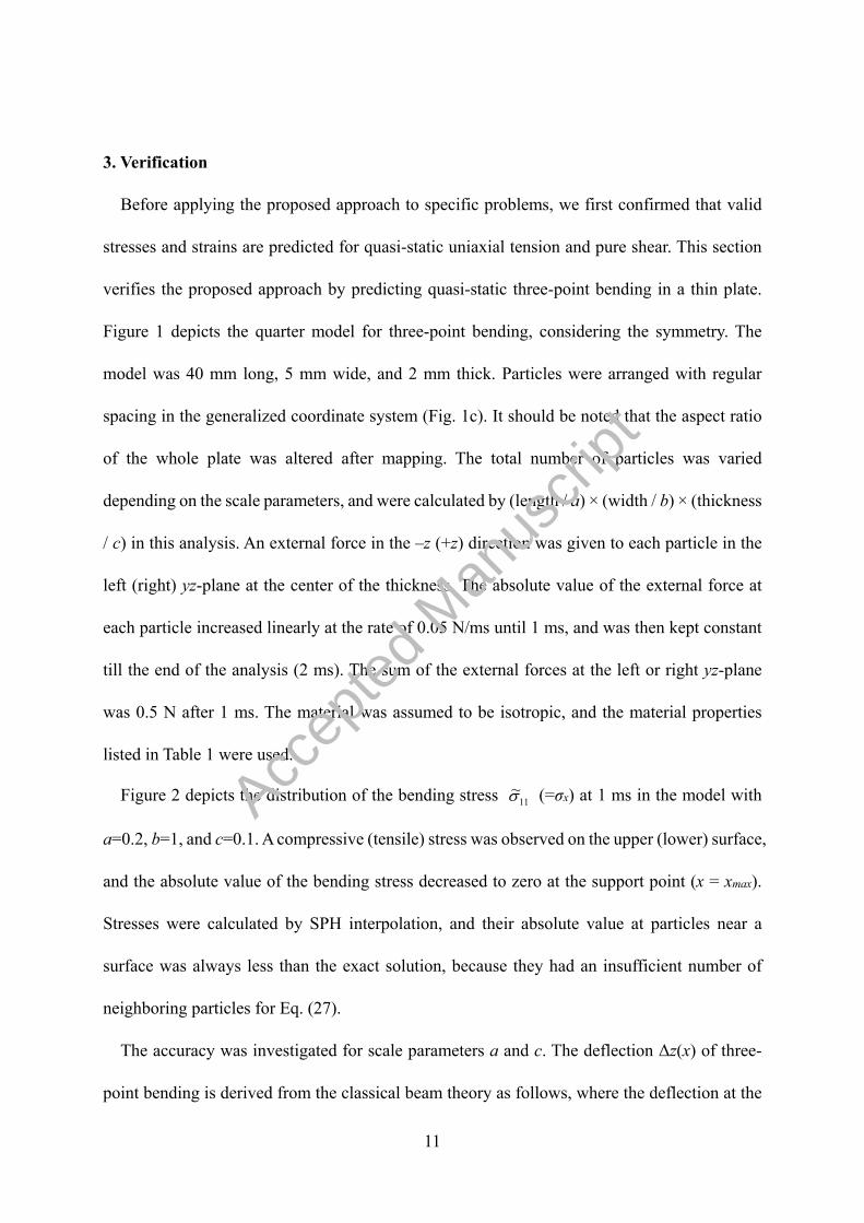
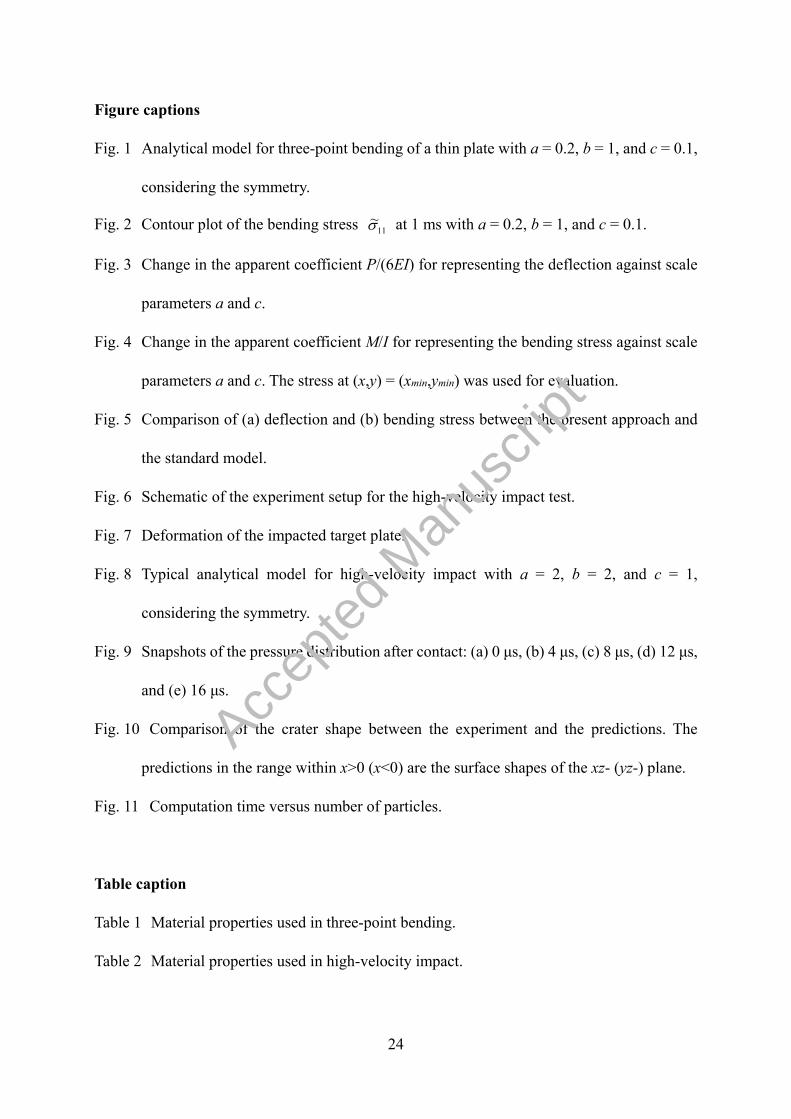
Figure 1 depicts the quarter model for three-point bending, considering the symmetry. The

model was 40 mm long, 5 mm wide, and 2 mm thick. Particles were arranged with regular

spacing in the generalized coordinate system (Fig. 1c). It should be noted that the aspect ratio

of the whole plate was altered after mapping. The total number of particles was varied

depending on the scale parameters, and were calculated by (length / a) × (width / b) × (thickness

/ c) in this analysis. An external force in the –z (+z) direction was given to each particle in the

left (right) yz-plane at the center of the thickness. The absolute value of the external force at

each particle increased linearly at the rate of 0.05 N/ms until 1 ms, and was then kept constant

till the end of the analysis (2 ms). The sum of the external forces at the left or right yz-plane

was 0.5 N after 1 ms. The material was assumed to be isotropic, and the material properties

listed in Table 1 were used.

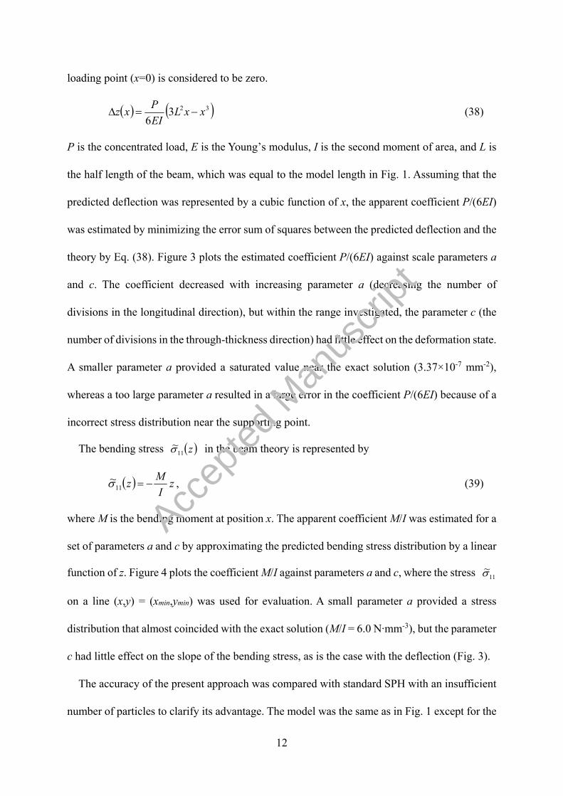
Figure 2 depicts the distribution of the bending stress 11~ (=σx) at 1 ms in the model with

a=0.2, b=1, and c=0.1. A compressive (tensile) stress was observed on the upper (lower) surface,

and the absolute value of the bending stress decreased to zero at the support point (x = xmax).

Stresses were calculated by SPH interpolation, and their absolute value at particles near a

surface was always less than the exact solution, because they had an insufficient number of

neighboring particles for Eq. (27).

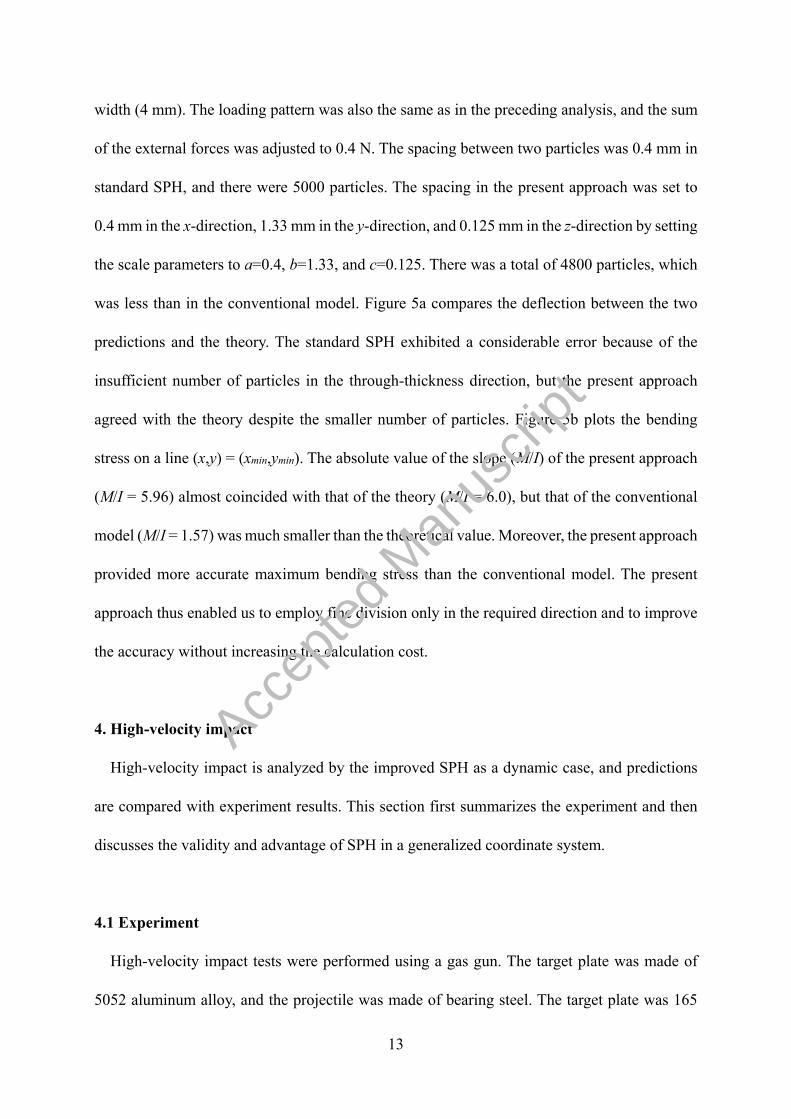
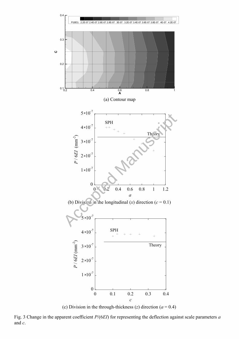
The accuracy was investigated for scale parameters a and c. The deflection Δz(x) of three-

point bending is derived from the classical beam theory as follows, where the deflection at the

Accep

ted

Man

uscr

ipt

12

loading point (x=0) is considered to be zero.

3236

xxLEI

Pxz (38)

P is the concentrated load, E is the Young’s modulus, I is the second moment of area, and L is

the half length of the beam, which was equal to the model length in Fig. 1. Assuming that the

predicted deflection was represented by a cubic function of x, the apparent coefficient P/(6EI)

was estimated by minimizing the error sum of squares between the predicted deflection and the

theory by Eq. (38). Figure 3 plots the estimated coefficient P/(6EI) against scale parameters a

and c. The coefficient decreased with increasing parameter a (decreasing the number of

divisions in the longitudinal direction), but within the range investigated, the parameter c (the

number of divisions in the through-thickness direction) had little effect on the deformation state.

A smaller parameter a provided a saturated value near the exact solution (3.37×10-7 mm-2),

whereas a too large parameter a resulted in a large error in the coefficient P/(6EI) because of a

incorrect stress distribution near the supporting point.

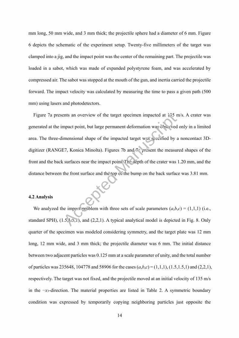
The bending stress z11~ in the beam theory is represented by

zI

Mz 11

~ , (39)

where M is the bending moment at position x. The apparent coefficient M/I was estimated for a

set of parameters a and c by approximating the predicted bending stress distribution by a linear

function of z. Figure 4 plots the coefficient M/I against parameters a and c, where the stress 11~

on a line (x,y) = (xmin,ymin) was used for evaluation. A small parameter a provided a stress

distribution that almost coincided with the exact solution (M/I = 6.0 N∙mm-3), but the parameter

c had little effect on the slope of the bending stress, as is the case with the deflection (Fig. 3).

The accuracy of the present approach was compared with standard SPH with an insufficient

number of particles to clarify its advantage. The model was the same as in Fig. 1 except for the

Accep

ted

Man

uscr

ipt

13

width (4 mm). The loading pattern was also the same as in the preceding analysis, and the sum

of the external forces was adjusted to 0.4 N. The spacing between two particles was 0.4 mm in

standard SPH, and there were 5000 particles. The spacing in the present approach was set to

0.4 mm in the x-direction, 1.33 mm in the y-direction, and 0.125 mm in the z-direction by setting

the scale parameters to a=0.4, b=1.33, and c=0.125. There was a total of 4800 particles, which

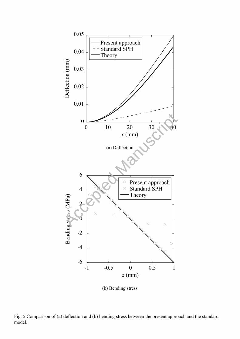
was less than in the conventional model. Figure 5a compares the deflection between the two

predictions and the theory. The standard SPH exhibited a considerable error because of the

insufficient number of particles in the through-thickness direction, but the present approach

agreed with the theory despite the smaller number of particles. Figure 5b plots the bending

stress on a line (x,y) = (xmin,ymin). The absolute value of the slope (M/I) of the present approach

(M/I = 5.96) almost coincided with that of the theory (M/I = 6.0), but that of the conventional

model (M/I = 1.57) was much smaller than the theoretical value. Moreover, the present approach

provided more accurate maximum bending stress than the conventional model. The present

approach thus enabled us to employ fine division only in the required direction and to improve

the accuracy without increasing the calculation cost.

4. High-velocity impact

High-velocity impact is analyzed by the improved SPH as a dynamic case, and predictions

are compared with experiment results. This section first summarizes the experiment and then

discusses the validity and advantage of SPH in a generalized coordinate system.

4.1 Experiment

High-velocity impact tests were performed using a gas gun. The target plate was made of

5052 aluminum alloy, and the projectile was made of bearing steel. The target plate was 165

Accep

ted

Man

uscr

ipt

14

mm long, 50 mm wide, and 3 mm thick; the projectile sphere had a diameter of 6 mm. Figure

6 depicts the schematic of the experiment setup. Twenty-five millimeters of the target was

clamped into a jig, and the impact point was the center of the remaining part. The projectile was

loaded in a sabot, which was made of expanded polystyrene foam, and was accelerated by

compressed air. The sabot was stopped at the mouth of the gun, and inertia carried the projectile

forward. The impact velocity was calculated by measuring the time to pass a given path (500

mm) using lasers and photodetectors.

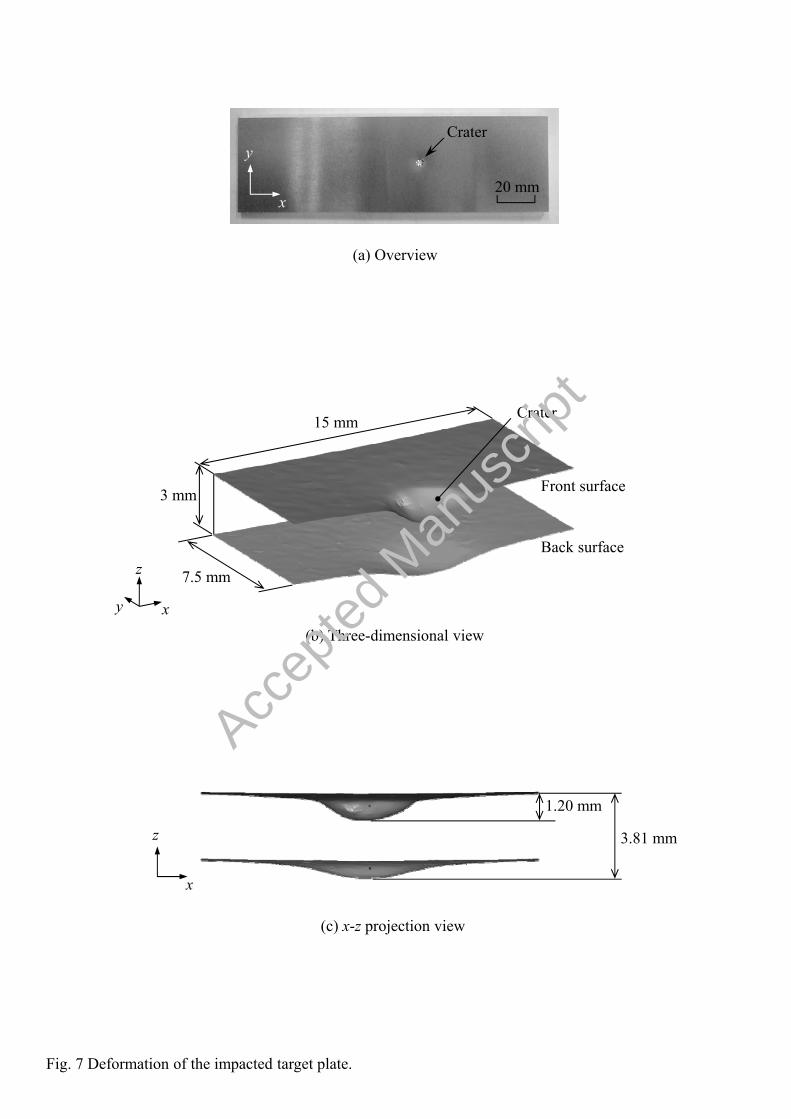
Figure 7a presents an overview of the target specimen impacted at 135 m/s. A crater was

generated at the impact point, but large permanent deformation was observed only in a limited

area. The three-dimensional shape of the impacted target was specified by a noncontact 3D-

digitizer (RANGE7, Konica Minolta). Figures 7b and 7c present the measured shapes of the

front and the back surfaces near the impact point. The depth of the crater was 1.20 mm, and the

distance between the front surface and the top of the bump on the back surface was 3.81 mm.

4.2 Analysis

We analyzed the impact problem with three sets of scale parameters (a,b,c) = (1,1,1) (i.e.,

standard SPH), (1.5,1.5,1), and (2,2,1). A typical analytical model is depicted in Fig. 8. Only

quarter of the specimen was modeled considering symmetry, and the target plate was 12 mm

long, 12 mm wide, and 3 mm thick; the projectile diameter was 6 mm. The initial distance

between two adjacent particles was 0.125 mm at a scale parameter of unity, and the total number

of particles was 235648, 104778 and 58906 for the cases (a,b,c) = (1,1,1), (1.5,1.5,1) and (2,2,1),

respectively. The target was not fixed, and the projectile moved at an initial velocity of 135 m/s

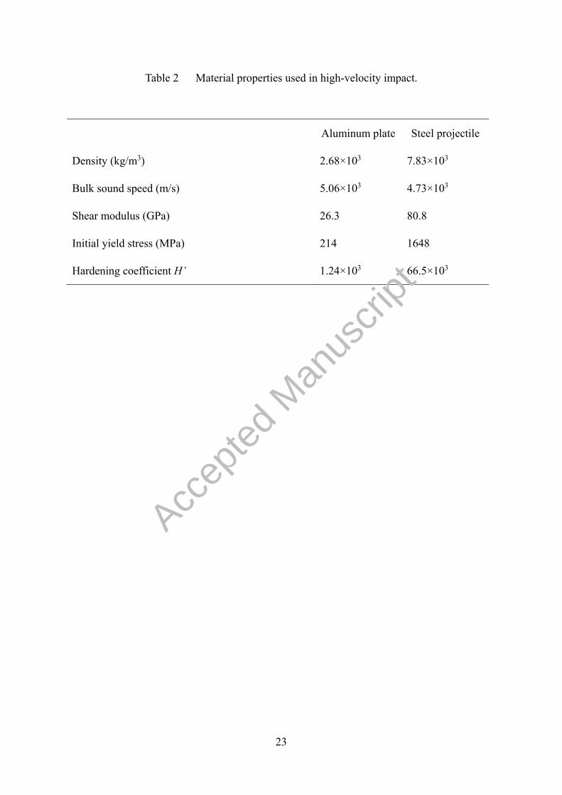
in the −x3-direction. The material properties are listed in Table 2. A symmetric boundary

condition was expressed by temporarily copying neighboring particles just opposite the

Accep

ted

Man

uscr

ipt

15

symmetry plane, and this handling was performed only in the particles whose effective range

exceeded that plane. It should be noted that sign inversion was required for some quantities of

the temporarily-copied particles.

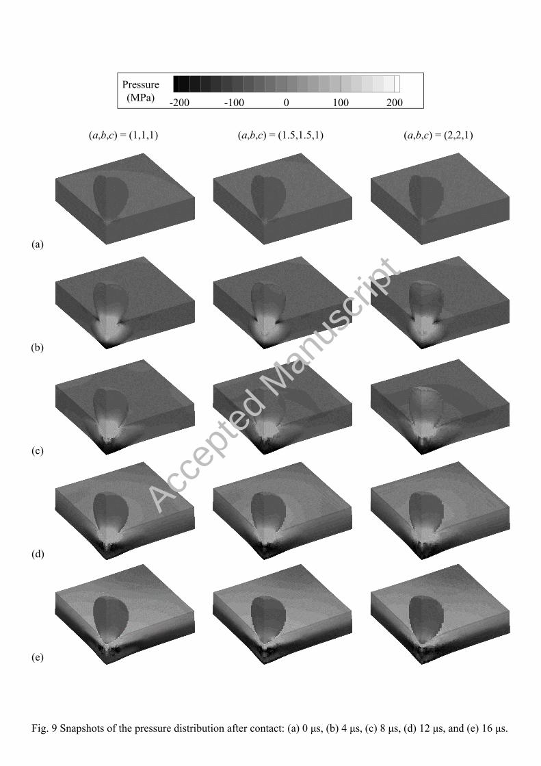
Figure 9 presents the pressure distribution predicted by the three models. These results agreed

well with each other, but the high-pressure region was broadened slightly by a greater scale

parameter. The effective radii of the three models were the same in the mathematical space, but

in the physical space, the effective ellipsoidal region became larger due to a greater scale

parameter. This may be the reason for the marginal discrepancy in the pressure distribution.

Figure 10 compares the deformation of the target between the experiment and the predictions

by the three models. The deformation obtained by standard SPH was generally consistent with

the measurement. Greater scale parameters also reproduced close crater shapes, but the depth

of the crater decreased with increasing scale parameters because the local high stresses were

smoothed in the x1x2-plane by increasing parameters a and b. There was a difference between

the measured final deformed shape and the predicted one. The major cause of this difference

will be the constitutive model. The classical elastic-plastic theory can describe the strain

hardening effect, but cannot consider effects of strain rate and temperature. A constitutive model

including these effects, e.g., Johnson-Cook viscoplastic model, will diminish the difference.

Finally, Fig. 11 presents the computation time versus the number of particles. The

computation time decreased as the 1.17th power of the number of particles. Compared with

standard SPH, i.e., (a,b,c) = (1,1,1), the present approach with scale parameters of (2,2,1) took

only 25% of the number of particles and 17% of the computation time. The characteristics of

this approach thus reduced the calculation cost by reducing the number of divisions in a

direction with a moderate change in the stress field.

Accep

ted

Man

uscr

ipt

16

5. Conclusions

This study proposed a numerical scheme of smoothed particle hydrodynamics (SPH) solving

in a generalized coordinate system. Particles were first allocated inhomogeneously in the

physical Cartesian coordinate system and then were arranged homogeneously in a generalized

coordinate system, thanks to the use of scaled base vectors. The governing equations were

solved in the generalized coordinate system, but the numerical scheme was the same as with

standard SPH. This study verified the present approach by investigating quasi-static three-point

bending of a thin plate and applied it to high-velocity impact problems. The conclusions are

summarized below.

1. The present approach with an adequate set of scale parameters significantly improved the

accuracy in the bending-stress distribution in a thin plate without increasing the calculation

cost, compared with standard SPH with an insufficient number of particles. The accuracy

in the bending-stress distribution was improved remarkably by employing fine division in

the longitudinal and through-thickness directions.

2. The predicted shape of the crater agreed well with the experiment measurement regardless

of the scale parameters. Moreover, the pressure distribution obtained by the present

approach coincided with that of standard SPH. These results confirmed the numerical

scheme of SPH in a generalized coordinate system.

3. The numerical results revealed that the calculation time decreased as the 1.17th power of

the number of particles. Unlike standard SPH, fine division occurs only in a required

direction, and this characteristic reduced the calculation cost by reducing the number of

divisions in a direction with a moderate change in the stress field.

Acknowledgments

Accep

ted

Man

uscr

ipt

17

S. Y. acknowledges the support of the Japan Society for the Promotion of Science (JSPS)

under Grants-in-Aid for Scientific Research (No. 25289306). S. Y. and T. O. also acknowledge

the support of the Japan Science and Technology Agency through Cross-ministerial Strategic

Innovation Promotion Program (SIP). The authors thank Mr. D. Komagata (Tohoku University)

and Mr. T. Ikawa (Shizuoka University) for their great efforts. The authors also express

appreciation to Dr. A. Yoshimura (Japan Aerospace Exploration Agency) for his support in the

experiment.

References

[1] Gingold RA, Monaghan JJ. Smoothed particle hydrodynamics: theory and application to

non-spherical stars. Monthly Notices of the Royal Astronomical Society 1977; 181:375-389.

[2] Lucy LB. A numerical approach to the testing of the fission hypothesis. Astronomical

Journal 1977; 82:1013-1024.

[3] Belytschko T, Lu YY, Gu L. Element-free Galerkin methods. International Journal for

Numerical Methods in Engineering 1994; 37:229-256.

[4] Liu WK, Jun S, Li S, Adee J, Belytschko T. Reproducing kernel particle methods for

structural dynamics. International Journal for Numerical Methods in Engineering 1995;

38:1655-1679.

[5] Atluri SN, Zhu T. A new Meshless Local Petrov-Galerkin (MLPG) approach in

computational mechanics. Computational Mechanics 1998; 22:117-127.

[6] Sulsky DL, Kaul A. Implicit dynamics in the material-point method. Computer Methods in

Applied Mechanics and Engineering 2004; 139:1137-1170.

[7] Bardenhagen S, Kober E. The generalized interpolation material point method. Computer

Modeling in Engineering & Sciences 2004; 5:477-495.

Accep

ted

Man

uscr

ipt

18

[8] Wallstedt PC, Guilkey JE. A weighted least squares particle-in-cell method for solid

mechanics. International Journal for Numerical Methods in Engineering 2011; 85:1687-

1704.

[9] Randles PW, Libersky LD. Normalized SPH with stress points. International Journal for

Numerical Methods in Engineering 2000; 48:1455-1462.

[10] Sanchez JJ, Randles PW. Dynamic failure simulation of quasi-brittle material in dual

particle dynamics. International Journal for Numerical Methods in Engineering 2012;

91:1227-1250.

[11] Li B, Habbal F, Ortiz M. Optimal transportation meshfree approximation schemes for fluid

and plastic flows. International Journal for Numerical Methods in Engineering 2010;

83:1541-1579.

[12] Rabczuk T, Gracie R, Song J-H, Belytschko T. Immersed particle method for fluid–

structure interaction. International Journal for Numerical Methods in Engineering 2010;

81:48-71.

[13] Nguyen VP, Rabczuk T, Bordas S, Duflot M. Meshless methods: A review and computer

implementation aspects. Mathematics and Computers in Simulation 2008; 79:763-813.

[14] Monaghan JJ. Simulating free surface flows with SPH. Journal of Computational Physics

1994; 110: 399-406.

[15] Takeda H, Miyama SM, Sekiya M. Numerical simulation of viscous flow by smoothed

particle hydrodynamics. Progress of Theoretical Physics 1994; 92:939-960.

[16] Morris JP, Fox PJ, Zhu Y. Modeling low Reynolds number incompressible flows using SPH.

Journal of Computational Physics 1997; 136:214-226.

[17] Lee ES, Moulinec C, Xu R, Violeau D, Laurence D, Stansby P. Comparisons of weakly

compressible and truly incompressible algorithms for the SPH mesh free particle method.

Accep

ted

Man

uscr

ipt

19

Journal of Computational Physics 2008; 227:8417-8436.

[18] Szewc K, Pozorski J, Minier JP. Analysis of the incompressibility constraint in the

smoothed particle hydrodynamics method. International Journal for Numerical Methods

in Engineering 2012; 92: 343-369.

[19] Libersky LD, Petschek AG, Carney TC, Hipp JR, Allahdadi FA. High strain Lagrangian

hydrodynamics: a three-dimensional SPH code for dynamic material response. Journal of

Computational Physics 1993; 109:67-75.

[20] Benz W, Asphaug E. Simulations of brittle solids using smooth particle hydrodynamics.

Computer Physics Communications 1995; 87:253-265.

[21] Johnson GR, Stryk RA, Beissel SR. SPH for high velocity impact computations. Computer

Methods in Applied Mechanics and Engineering 1996; 139:347-373.

[22] Randles PW, Libersky LD. Smoothed particle hydrodynamics: some recent improvements

and applications. Computer Methods in Applied Mechanics and Engineering 1996;

139:375-408.

[23] Gray JP, Monaghan JJ, Swift RP. SPH elastic dynamics. Computer Methods in Applied

Mechanics and Engineering 2001; 190:6641-6662.

[24] Antoci C, Gallati M, Sibilla S. Numerical simulation of fluid-structure interaction by SPH.

Computers & Structures 2007; 85:879-890.

[25] Rafiee A, Thiagarajan KP. An SPH projection method for simulating fluid-hypoelastic

structure interaction. Computer Methods in Applied Mechanics and Engineering 2009;

198:2785-2795.

[26] Lee M, Yoo YH. Analysis of ceramic/metal armour systems. International Journal of

Impact Engineering 2001; 25:819-829.

[27] Shintate K, Sekine H. Numerical simulation of hypervelocity impacts of a projectile on

Accep

ted

Man

uscr

ipt

20

laminated composite plate targets by means of improved SPH method. Composites Part A

2004; 35:683-692.

[28] Michel Y, Chevalier JM, Durin C, Espinosa C, Malaise F, Barrau JJ. Hypervelocity impacts

on thin brittle targets: Experimental data and SPH simulations. International Journal of

Impact Engineering 2006; 33:441-451.

[29] Takaffoli M, Papini M. Material deformation and removal due to single particle impacts on

ductile materials using smoothed particle hydrodynamics. Wear 2012; 274-275:50-59.

[30] Cleary PW, Ha J, Prakash M, Nguyen T. 3D SPH flow predictions and validation for high

pressure die casting of automotive components. Applied Mathematical Modelling 2006;

30:1406-1427.

[31] Cleary PW, Prakash M, Das R, Ha J. Modelling of metal forging using SPH. Applied

Mathematical Modelling 2012; 36:3836-3855.

[32] Lee ES, Violeau D, Issa R, Ploix S. Application of weakly compressible and truly

incompressible SPH to 3-D water collapse in waterworks. Journal of Hydraulic Research

2010; 48:50-60.

[33] Gray JP, Monaghan JJ. Numerical modelling of stress fields and fracture around magma

chambers. Journal of Volcanology and Geothermal Research 2004; 135:259-283.

[34] Prakash M, Cleary PW, Three dimensional modelling of lava flow using smoothed particle

hydrodynamics. Applied Mathematical Modelling 2011; 35:3021-3035.

[35] Monaghan JJ. Smoothed particle hydrodynamics. Reports on Progress in Physics 2005;

68:1703-1759.

[36] Liu MB, Liu GR. Smoothed particle hydrodynamics (SPH): an overview and recent

developments. Archives of Computational Methods in Engineering 2010; 17:25-76.

[37] Wong S, Shie Y. Galerkin based smoothed particle hydrodynamics. Computers &

Accep

ted

Man

uscr

ipt

21

Structures 2009; 87:1111-1118.

[38] Herreros MI, Mabssout M. A two-steps time discretization scheme using the SPH method

for shock wave propagation. Computer Methods in Applied Mechanics and Engineering

2011; 200:1833-1845.

[39] Blanc T, Pastor M. A stabilized Runge–Kutta, Taylor smoothed particle hydrodynamics

algorithm for large deformation problems in dynamics. International Journal for

Numerical Methods in Engineering 2012; 91:1427-1458.

[40] Colagrossi A, Bouscasse B, Antuono M, Marronea S. Particle packing algorithm for SPH

schemes. Computer Physics Communications 2012; 183:1641-1653.

[41] Vacondio R, Rogers BD, Stansby PK, Mignosa P, Feldman J. Variable resolution for SPH:

A dynamic particle coalescing and splitting scheme. Computer Methods in Applied

Mechanics and Engineering 2013; 256:132-148.

[42] Puri K, Ramachandran P. A comparison of SPH schemes for the compressible Euler

equations. Journal of Computational Physics 2014; 256:308-333.

[43] Maurel B, Combescure A. An SPH shell formulation for plasticity and fracture analysis in

explicit dynamics. International Journal for Numerical Methods in Engineering 2008;

76:949-971.

[44] Caleyron F, Combescure A, Faucher V, Potapov S. Dynamic simulation of damage-fracture

transition in smoothed particles hydrodynamics shells. International Journal for Numerical

Methods in Engineering 2012; 90:707-738.

[45] Yashiro S, Ogi K, Yoshimura A, Sakaida Y. Characterization of high-velocity impact

damage in CFRP laminates: Part II – prediction by smoothed particle hydrodynamics.

Composites Part A 2014; 56:308-318.

Accep

ted

Man

uscr

ipt

22

Table 1 Material properties used in three-point bending.

Density (kg/m3) 2.785×103

Bulk sound speed (m/s) 5.328×103

Shear modulus (GPa) 27.6

Young’s modulus (GPa) 74.2

Poisson’s ratio 0.344

Accep

ted

Man

uscr

ipt

23

Table 2 Material properties used in high-velocity impact.

Aluminum plate Steel projectile

Density (kg/m3) 2.68×103 7.83×103

Bulk sound speed (m/s) 5.06×103 4.73×103

Shear modulus (GPa) 26.3 80.8

Initial yield stress (MPa) 214 1648

Hardening coefficient H’ 1.24×103 66.5×103

Accep

ted

Man

uscr

ipt

24

Figure captions

Fig. 1 Analytical model for three-point bending of a thin plate with a = 0.2, b = 1, and c = 0.1,

considering the symmetry.

Fig. 2 Contour plot of the bending stress 11~ at 1 ms with a = 0.2, b = 1, and c = 0.1.

Fig. 3 Change in the apparent coefficient P/(6EI) for representing the deflection against scale

parameters a and c.

Fig. 4 Change in the apparent coefficient M/I for representing the bending stress against scale

parameters a and c. The stress at (x,y) = (xmin,ymin) was used for evaluation.

Fig. 5 Comparison of (a) deflection and (b) bending stress between the present approach and

the standard model.

Fig. 6 Schematic of the experiment setup for the high-velocity impact test.

Fig. 7 Deformation of the impacted target plate.

Fig. 8 Typical analytical model for high-velocity impact with a = 2, b = 2, and c = 1,

considering the symmetry.

Fig. 9 Snapshots of the pressure distribution after contact: (a) 0 μs, (b) 4 μs, (c) 8 μs, (d) 12 μs,

and (e) 16 μs.

Fig. 10 Comparison of the crater shape between the experiment and the predictions. The

predictions in the range within x>0 (x<0) are the surface shapes of the xz- (yz-) plane.

Fig. 11 Computation time versus number of particles.

Table caption

Table 1 Material properties used in three-point bending.

Table 2 Material properties used in high-velocity impact.

Accep

ted

Man

uscr

ipt

Fig. 1 Analytical model for three-point bending of a thin plate with a = 0.2, b = 1, and c = 0.1, considering the symmetry.

(a) Schematic

40

2

5Unit: mm

(c) Particle-model in the mathematical space

θ1

θ3θ2

Plane of symmetry

(b) Particle-model in the physical space

x

zy

Accep

ted

Man

uscr

ipt

Fig. 2 Contour plot of the bending stress at 1 ms with a = 0.2, b = 1, and c = 0.1.

(MPa)

11~

Accep

ted

Man

uscr

ipt

A

C

0.2 0.4 0.6 0.8 10.1

0.2

0.3

0.4

P/(6EI): 2.2E-07 2.4E-07 2.6E-07 2.8E-07 3E-07 3.2E-07 3.4E-07 3.6E-07 3.8E-07 4E-07 4.2E-07

Fig. 3 Change in the apparent coefficient P/(6EI) for representing the deflection against scale parameters aand c.

(a) Contour map

(c) Division in the through-thickness (z) direction (a = 0.4)

0

1 10-7

2 10-7

3 10-7

4 10-7

5 10-7

0 0.2 0.4 0.6 0.8 1 1.2

P /

6EI

(m

m-2

)

a

×

Theory

SPH

×

×

×

×

(b) Division in the longitudinal (x) direction (c = 0.1)

0

1 10-7

2 10-7

3 10-7

4 10-7

5 10-7

0 0.1 0.2 0.3 0.4

P /

6EI

(mm

-2)

c

×

Theory

SPH

×

×

×

×

Accep

ted

Man

uscr

ipt

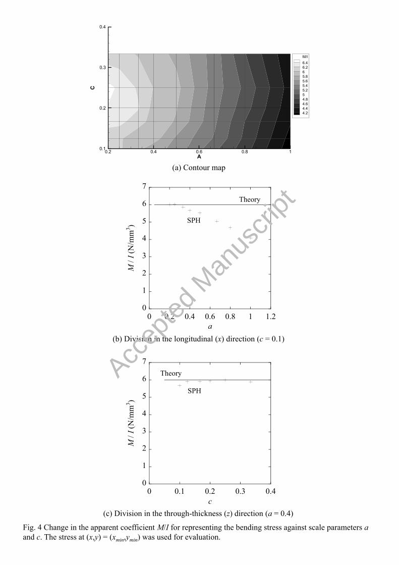
Fig. 4 Change in the apparent coefficient M/I for representing the bending stress against scale parameters aand c. The stress at (x,y) = (xmin,ymin) was used for evaluation.

0

1

2

3

4

5

6

7

0 0.2 0.4 0.6 0.8 1 1.2

M /

I (N

/mm

3 )

a

Theory

SPH

A

C

0.2 0.4 0.6 0.8 10.1

0.2

0.3

0.4

M/I

6.46.265.85.65.45.254.84.64.44.2

(a) Contour map

(c) Division in the through-thickness (z) direction (a = 0.4)

(b) Division in the longitudinal (x) direction (c = 0.1)

0

1

2

3

4

5

6

7

0 0.1 0.2 0.3 0.4

M /

I (N

/mm

3 )

c

Theory

SPH

Accep

ted

Man

uscr

ipt

(a) Deflection

(b) Bending stress

Fig. 5 Comparison of (a) deflection and (b) bending stress between the present approach and the standard model.

0

0.01

0.02

0.03

0.04

0.05

0 10 20 30 40

Present approachStandard SPHTheory

Def

lect

ion

(mm

)

x (mm)

-6

-4

-2

0

2

4

6

-1 -0.5 0 0.5 1

Present approachStandard SPHTheory

Ben

ding

str

ess

(MP

a)

z (mm)

Accep

ted

Man

uscr

ipt

Fig. 6 Schematic of the experiment setup for the high-velocity impact test

Laser*

Laser*

Photodetector #1

Photodetector #2

Sabot stopper

Target

ProjectilePressure tank

Accep

ted

Man

uscr

ipt

Crater

(a) Overview

20 mm

Back surface

15 mm

3 mm

7.5 mm

Crater

Front surface

x

y

z

xy

1.20 mm

3.81 mm

(c) x-z projection view

x

z

(b) Three-dimensional view

Fig. 7 Deformation of the impacted target plate.

Accep

ted

Man

uscr

ipt

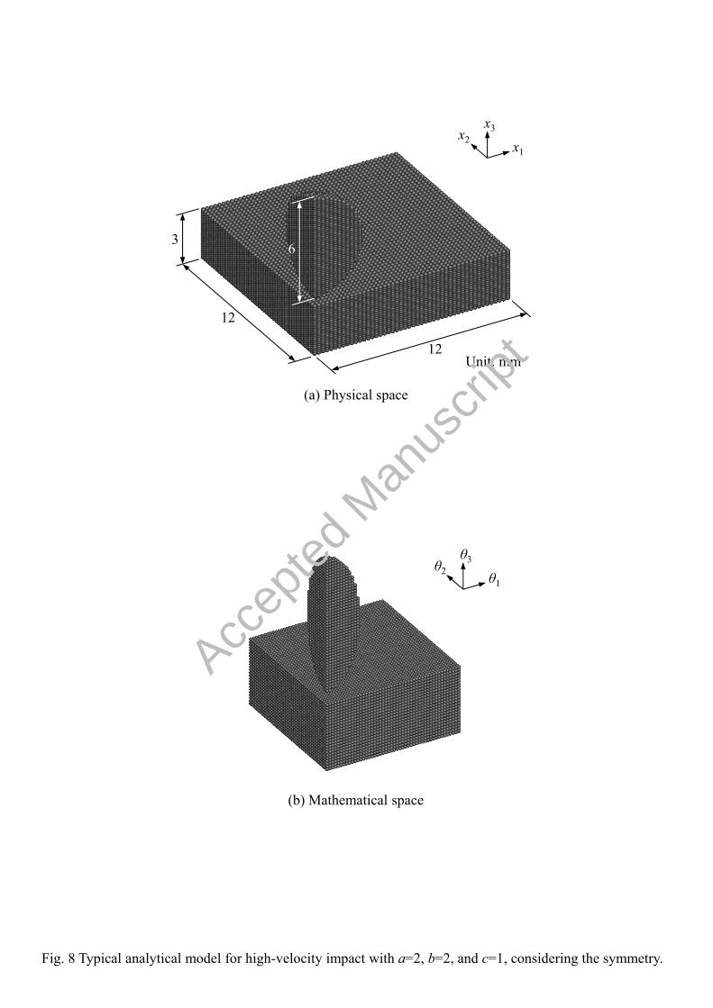
Fig. 8 Typical analytical model for high-velocity impact with a=2, b=2, and c=1, considering the symmetry.

(b) Mathematical space

(a) Physical space

3

12

12

x1

x2

x3

θ1

θ2

θ3

6

Unit: mm

Accep

ted

Man

uscr

ipt

Pressure(MPa) -200 -100 0 100 200

(a)

Fig. 9 Snapshots of the pressure distribution after contact: (a) 0 μs, (b) 4 μs, (c) 8 μs, (d) 12 μs, and (e) 16 μs.

(a,b,c) = (1,1,1) (a,b,c) = (1.5,1.5,1) (a,b,c) = (2,2,1)

(b)

(c)

(d)

(e)

Accep

ted

Man

uscr

ipt

(Front)

(Back)

(a,b,c) = (2,2,1)(a,b,c) = (1.5,1.5,1)(a,b,c) = (1,1,1)Experiment

Fig. 10 Comparison of the crater shape between the experiment and the predictions. The predictions in the range within x > 0 (x < 0) are the surface shapes of the xz- (yz-) plane.

-4-3-2-101

-7.5 0 7.5

Dis

plac

emen

t (m

m)

x (mm)

Accep

ted

Man

uscr

ipt

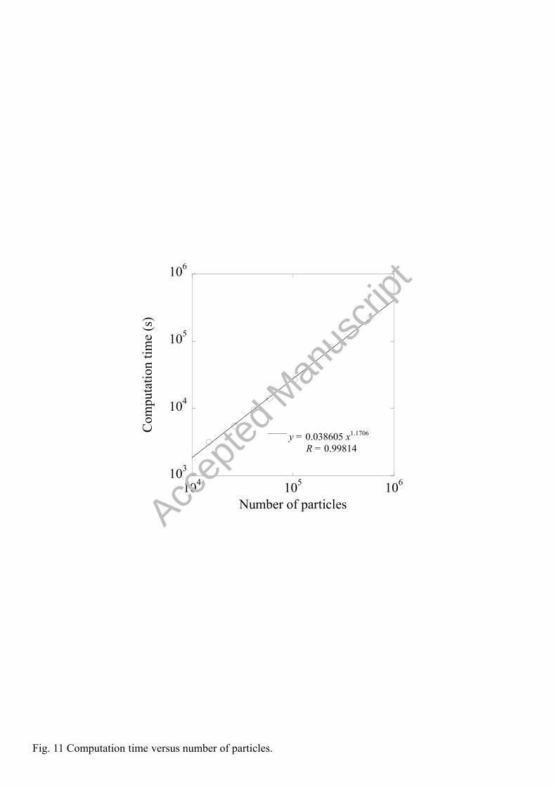
Fig. 11 Computation time versus number of particles.

103

104

105

106

104 105 106

y = 0.038605 x1.1706

R = 0.99814

Com

puta

tion

tim

e (s

)

Number of particlesAccep

ted

Man

uscr

ipt