Embed Size (px)
Citation preview
A time-varying parameter structural model of the UK economy
Accepted Manuscript
A time-varying parameter structural model of the UK economy
George Kapetanios, Riccardo M. Masolo, Katerina Petrova,Matthew Waldron
PII: S0165-1889(19)30092-2DOI: https://doi.org/10.1016/j.jedc.2019.05.012Reference: DYNCON 3705
To appear in: Journal of Economic Dynamics & Control
Received date: 30 July 2018Revised date: 18 March 2019Accepted date: 24 May 2019
Please cite this article as: George Kapetanios, Riccardo M. Masolo, Katerina Petrova,Matthew Waldron, A time-varying parameter structural model of the UK economy, Journal ofEconomic Dynamics & Control (2019), doi: https://doi.org/10.1016/j.jedc.2019.05.012
This is a PDF file of an unedited manuscript that has been accepted for publication. As a serviceto our customers we are providing this early version of the manuscript. The manuscript will undergocopyediting, typesetting, and review of the resulting proof before it is published in its final form. Pleasenote that during the production process errors may be discovered which could affect the content, andall legal disclaimers that apply to the journal pertain.

ACCEPTED MANUSCRIPT
ACCEPTED MANUSCRIP
T
A time-varying parameter structural model of the UK economy∗
George Kapetanios† Riccardo M. Masolo‡§ Katerina Petrova¶‖ Matthew Waldron¶
March 17, 2019
Abstract
We estimate a time-varying parameter structural macroeconomic model of the UK economy,
using a Bayesian local likelihood methodology. This enables us to estimate a large open-economy
DSGE model over a sample that comprises several different monetary policy regimes and an
incomplete set of data. Our estimation identifies a gradual shift to a monetary policy regime
characterised by an increased responsiveness of policy towards inflation alongside a decrease in
the inflation trend down to the two percent target level. The time-varying model also performs
remarkably well in forecasting and delivers statistically significant accuracy improvements for
most variables and horizons for both point and density forecasts compared to the standard
fixed-parameter version.
JEL codes: C11, C53, E27, E52
Keywords: DSGE models, open economy, time varying parameters, UK economy
∗Any views expressed are solely those of the authors and so, cannot be taken to represent those of the Bank of
England or any of its policy committees, or to state Bank of England’s policy.†School of Management and Business, King’s College, London‡Bank of England§Centre for Macroeconomics, London¶University of St Andrews‖Corresponding author, Email: [email protected]
1
ACCEPTED MANUSCRIPT
ACCEPTED MANUSCRIP
T
1 Introduction
Dynamic stochastic general equilibrium (DSGE) models have become popular tools for macroeco-
nomic analysis and forecasting. Their success is the result of their capacity to combine macro-
economic theory with a reasonable data fit to business cycle fluctuations and a relatively good
forecasting performance. Developments in Bayesian methods coupled with innovations in comput-
ing have made it possible for medium to large DSGE models to be easily estimated.
An assumption underpinning standard Bayesian estimation of DSGE models, such as the one
presented in Smets and Wouters (2007), is that the parameters of the model are constant over
time. While over relatively short samples or monotonous periods, this is a reasonable assumption,
over longer samples and periods characterised by structural change, it is unlikely to hold. For the
United Kingdom, there are a-priori reasons to believe that the structure of the economy has changed
substantially in recent decades and, as a result, the assumption that the parameters of a DSGE
model for the UK economy have remained constant is unrealistic. More specifically, we have recently
seen a period of considerable changes to the labour market in the UK (e.g. declining unionisation),
a large-scale shift in production from manufacturing towards services, substantive changes to the
financial sector following the deregulation of the mid-1980s and the recent financial crisis, and a
rapid expansion in world trade. Recent changes also include several significant adjustments to
the conduct of monetary policy, beginning with intermediate monetary aggregate targetting in the
1970s, followed by exchange rate targetting, which was formalised in 1989 when the UK entered
the Exchange Rate Mechanism (ERM), and ending with inflation targetting —first conducted by
the UK government and then by the Monetary Policy Committee of the Bank of England. In this
context, it is very diffi cult to justify the assumption that the structural parameters of a model
describing the UK economy have remained constant over the past several decades.
In this paper, we investigate structural change in the UK economy by estimating a structural
DSGE model using a methodology that allows for parameters to vary over time. The model we
choose is the small open economy DSGE model developed by Burgess, Fernandez-Corugedo, Groth,
Harrison, Monti, Theodoridis and Waldron (2013), referred to as COMPASS. It was designed by
Bank of England economists for policy analysis and forecasting and it bears similarities to other
open-economy models used in policy institutions, such as Adolfson, Andersson, Linde, Villani and
Vredin (2007). Reflecting on the brief discussion of recent UK monetary history above, Burgess
et al. (2013) restrict the estimation sample to the 1993Q1-2007Q4 period that begins after the
adoption of inflation targetting and ends before the Great Recession1. This has the drawback of
being a relatively short sample (e.g. compared to similar studies on US data) and may not be
1Due to the challenges discussed, there are only a handful of papers similar to ours in scope. Harrison and
Oomen (2010) can be considered a predecessor of Burgess et al. (2013), while DiCecio and Nelson (2007) estimates
a closed-economy model.
2
ACCEPTED MANUSCRIPT
ACCEPTED MANUSCRIP
T
representative (with implications for forecasting), given that it only incorporates data from the
Great Moderation. We address this shortcoming by extending the sample backwards to 1975, and
forwards to 2014.
The literature on estimating reduced form models such as vector autoregressions with time-
variation in the parameters includes well-known papers such as Cogley and Sargent (2002), Prim-
iceri (2005), Cogley and Sbordone (2008), Benati and Surico (2009), Gali and Gambetti (2009),
Canova and Gambetti (2009) and Mumtaz and Surico (2009)2. The literature on DSGE models
with drifts in the parameters is less developed, due to: (i) the additional complexity that arises
from the algorithms used for the solution and estimation of these models, and (ii) the additional
assumptions required about the way the agents in the model form expectations about the future
parameter values. One way in which time-variation in the parameters of a DSGE model has been
modelled is by specifying stochastic processes known to agents in the model for a subset of the pa-
rameters (e.g. Justiniano and Primiceri (2008), Fernandez-Villaverde and Rubio-Ramirez (2008)).
For instance, Fernandez-Villaverde and Rubio-Ramirez (2008) assume that agents in the model take
into account future parameter variation when forming their expectations. Similar assumptions are
made by Schorfheide (2005), Bianchi (2013), Foerster, Rubio-Ramirez, Waggoner and Zha (2014),
but the parameters are modelled as Markov-switching processes. There are two drawbacks from
this approach. First, for every time-varying parameter, the state vector is augmented and an addi-
tional shock is introduced, which increases the complexity of the DSGE model and is subject to the
‘curse of dimensionality’, so that only a small subset of the model’s parameters can be modelled
in this way. Second, it imposes additional structure by relying on the assumption that the law of
motion for the parameters’time-variation is correctly specified3.
In contrast, Canova (2006), Canova and Sala (2009) and Castelnuovo (2012) allow for parameter
variation by estimating DSGE models over rolling samples. When applied to structural models,
the rolling window approach assumes that, instead of being endowed with perfect knowledge about
the economy’s data generating process, agents take parameter variation as exogenous when forming
their expectations about the future. This assumption facilitates estimation and can be rationalised
from the perspective of models featuring learning. In recent work, Galvão, Giraitis, Kapetanios
and Petrova (2019) propose a new methodology that makes the time-varying Bayesian estimation
of large structural models possible, as demonstrated by the estimation of a Smets and Wouters
(2007) DSGE model in Galvão et al. (2016, 2019). Their approach is an extension and formalisa-
tion of rolling window estimation, generalised by combining kernel-generated local likelihoods with
2One example of a paper that considers a similar research question to ours is Ellis, Mumtaz and Zabczyk (2014)
who use a time-varying factor augmented VAR to study structural changes in the transmission of monetary policy
shocks in the UK.3Petrova (2019b) shows in a Monte Carlo exercise that treating parameters as state variables when the law of
motion is misspecified may result in invalid estimates of the parameters’time variation, even asymptotically.
3

ACCEPTED MANUSCRIPT
ACCEPTED MANUSCRIP
T
appropriately chosen priors to generate a sequence of posterior distributions for the parameters
over time, following the methodology developed in Giraitis, Kapetanios and Yates (2014), Giraitis,
Kapetanios, Wetherilt and Zikes (2016) and Petrova (2019b). The advantages of the kernel method
are: (i) it does not require parametric assumptions about the parameters’ law of motion and it
performs well for many different deterministic and stochastic processes, and (ii) it allows for esti-
mation of time variation in all DSGE parameters. Moreover, Galvão et al. (2019) prove that, when
restricting attention to slowly varying parameter processes, the likelihood of the observables in a
particular period in a linear DSGE model only depends on the parameters at that period, ensuring
that standard algorithms can be used to facilitate the consistent estimation of the slowly drifting
parameter process.
In this paper, we employ the Galvão et al. (2019) approach and apply it to COMPASS to
investigate the structural nature of the parameters of the model. The flexibility of the approach in
the face of structural change permits the estimation of COMPASS over a longer period, alleviating
the need to restrict the sample to post-1992 and pre-crisis data. Given that this approach is based
on the Kalman filter, it also allows us to deal with missing observations, which is necessary due to
unavailability of some series required for COMPASS prior to 1987.
One additional methodological contribution of the paper is to develop further the QBLL method-
ology in order to handle estimation of mixtures of constant and time-varying parameters in the
linear DSGE setup. This requires the design of new block-Metropolis and Metropolis-within-Gibbs
algorithms suited to sample from the posteriors of mixtures of time-invariant and time-varying
parameters.
Our empirical results are noteworthy for several reasons. First, our estimates clearly show
evidence of time-variation in the parameters which translates into changes in the transmission
of shocks as well as in the evolution and relative importance of structural shocks. Second, we
demonstrate that our time-varying model outperforms its constant-parameter counterpart when it
comes to forecasting, which is important since forecasting is one of the main uses of COMPASS in
the Bank of England (Burgess et al. (2013)). Finally, when we estimate the constant parameter
model with changing volatility with the Metropolis-within-Gibbs algorithm we find better in- and
out-of-sample fit compared to the standard version of the model where all parameters are constant,
but worse performance compared to the model in which all parameters are allowed to vary, leading
to the conclusion that not only changes to the volatility are evident in the UK data over the sample,
but also changes in the parameters guiding the macroeconomic relations in the model.
The remainder of the paper is organised as follows. Section 2 describes the quasi-Bayesian local
likelihood approach of Galvão et al. (2019) and develops the novel block-Metropolis algorithm,
Section 3 presents COMPASS, Section 4 contains the empirical results and forecasting comparison
and Section 5 concludes.
4
ACCEPTED MANUSCRIPT
ACCEPTED MANUSCRIP
T
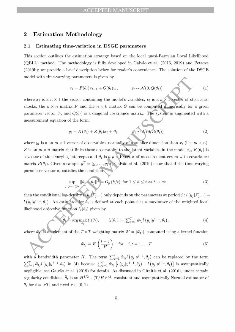
2 Estimation Methodology
2.1 Estimating time-variation in DSGE parameters
This section outlines the estimation strategy based on the local quasi-Bayesian Local Likelihood
(QBLL) method. The methodology is fully developed in Galvão et al. (2016, 2019) and Petrova
(2019b); we provide a brief description below for reader’s convenience. The solution of the DSGE
model with time-varying parameters is given by
xt = F (θt)xt−1 +G(θt)vt, vt ∼ N (0, Q(θt)) (1)
where xt is a n × 1 the vector containing the model’s variables, vt is a k × 1 vector of structural
shocks, the n × n matrix F and the n × k matrix G can be computed numerically for a given
parameter vector θt, and Q(θt) is a diagonal covariance matrix. The system is augmented with a
measurement equation of the form:
yt = K(θt) + Z(θt)xt + ϑt, ϑt ∼ N (0, R(θt)) (2)
where yt is a an m× 1 vector of observables, normally of a smaller dimension than xt (i.e. m < n),
Z is an m× n matrix that links those observables to the latent variables in the model xt, K(θt) is
a vector of time-varying intercepts and ϑt is a p× 1 vector of measurement errors with covariance
matrix R(θt). Given a sample yT = (y1, ..., yT ) , Galvão et al. (2019) show that if the time-varying
parameter vector θt satisfies the condition
supj:|j−t|≤h
||θt − θj ||2 = Op (h/t) for 1 ≤ h ≤ t as t→∞, (3)
then the conditional log-density l (yj |Fj−1) only depends on the parameters at period j : l (yj |Fj−1) =
l(yj |yj−1, θj
). An estimator for θt is defined at each point t as a maximiser of the weighted local
likelihood objective function `t(θt) given by
θt = arg maxθt
`t(θt), `t(θt) :=∑T
j=1 wtjl(yj |yj−1, θt
), (4)
where wtj is an element of the T ×T weighting matrixW = [wtj ], computed using a kernel function
wtj = K
(t− jH
)for j, t = 1, ..., T (5)
with a bandwidth parameter H. The term∑T
j=1 wtjl(yj |yj−1, θj
)can be replaced by the term∑T
j=1 wtjl(yj |yj−1, θt
)in (4) because
∑Tj=1 wtj
[l(yj |yj−1, θj
)− l(yj |yj−1, θt
)]is asymptotically
negligible; see Galvão et al. (2019) for details. As discussed in Giraitis et al. (2016), under certain
regularity conditions, θt is an H1/2 + (T/H)1/2- consistent and asymptotically Normal estimator of
θt for t = [τT ] and fixed τ ∈ (0, 1) .
5
ACCEPTED MANUSCRIPT
ACCEPTED MANUSCRIP
T
There are important reasons for adopting a Bayesian framework when considering DSGE mod-
els: priors can resolve issues such as non-concave likelihoods or ill-identified parameters due to small
sample sizes, and additionally, the Bayesian approach offers a combination between estimation and
calibration methods widely used in earlier models (e.g. Kydland and Prescott (1996)). The ker-
nel approach above is extended to Bayesian problems by Petrova (2019b), who shows that the
resulting quasi-posterior distributions are asymptotically Normal and valid for confidence interval
construction as long as the weights wtj in (4) are replaced by
wtj =(∑T
j=1 w2tj
)−1 (wtj/
∑Tj=1 wtj
)for j, t = 1, ..., T. (6)
The normalisation in (6) is employed to maintain the relative balance between the likelihood and the
prior and to obtain the same rate of convergence as in the frequentist work of Giraitis et al. (2014).
More formally, the local likelihood of the DSGE model in (4) with the modified kernel weights in
(6) at each period t is augmented with the prior distribution of the structural parameters, p(θt),
to get the quasi-posterior4 at time t, pt(θt|Y ):
pt(θt|yT ) =pt(θt) exp(`t(θt))∫
Θpt(θt) exp(`t(θt))dθ. (7)
Because the model has a linear Gaussian state space representation in equations (1) and (2), in
order to evaluate `t(θt), standard Kalman filter recursions can be employed to recursively compute
lj(yj |yj−1, θt
), which are kernel-weighted through (4), combined with a prior density through (7),
and, finally, passed to a numerical optimisation routine or posterior simulation algorithm. To
obtain the sequence of time-varying quasi-posterior densities pt(θt|yT ), it is easy to modify the
Metropolis-Hastings algorithm to include the kernel weights. Detailed outline of the algorithm can
be found in Galvão et al. (2019). Here we include a brief outline of the algorithm for reference and
reader’s convenience. At each t the algorithm implements the following steps.
Time-varying random walk Metropolis algorithm.
Step 1. The posterior is log-linearised and optimisation with respect to θ is performed to
obtain the posterior mode:
θt = arg minθt
(−∑T
j=1wtjl(yj |yj−1, θt
)− log p(θt)
).
Step 2. The inverse of the negative Hessian, Σt, is computed numerically, evaluated at the
posterior mode, θt.
Step 3. A starting value θ0t is drawn from N (θt, c
20Σt). For i = 1, ..., nsim, ζt is drawn from the
proposal distribution N (θ(i−1)t , c2Σt), where c2
0 and c2 are scaling parameters adjusting the step size
4The reason why Petrova (2018) adopts the term ‘quasi-posterior’is that the local likelihood in (4) is not a proper
density because of the kernel weights.
6

ACCEPTED MANUSCRIPT
ACCEPTED MANUSCRIP
T
of the algorithm in order to obtain satisfactory rejection rates. The following statistic is computed
r(θi−1t , ζt|yT ) =
exp(∑T
j=1wtjl(yj |yj−1, ζt
))p(ζt)
exp(∑T
j=1wtjl(yj |yj−1, θi−1
t
))p(θi−1
t ),
which is the ratio between the weighted quasi-posterior at the proposal ζt and θi−1t . The draw θ(i−1)
t
is accepted (setting θit = ζt) with probability τit = min1, r(θ(i−1)
t , ζt|y1:T ) and rejected (θi−1t = θit)
with probability 1− τ it.For generating DSGE-based predictions, our method uses the quasi-posterior at the end of the
sample p(θt=T |yT ), since this contains the most relevant information for prediction. At period
T , the kernel is one-sided and backward looking, so the posterior at T is computed using only
information up to T . For more formal discussion of how the method can be used for forecasting
as well as different forecasting schemes, we refer the reader to Galvão et al. (2019). We include a
brief description of the algorithm for computing the predictive densities p(yT+h|yT ) in Section 6.1
of the Appendix.
2.2 Estimation of mixtures of time-varying and time-invariant parameters
There are cases when only a subset of the parameters are varying over time. In these cases, the
estimators in Section 2.1 are still valid for estimation, since a constant parameter is a special case
of the processes covered by the condition in (3). However, since the kernel-weighted estimator
delivers consistency at a slower nonparametric rate, being able to estimate the subset of constant
parameters in a time-invariant fashion can provide effi ciency gains compared to the benchmark
estimation where all parameters are varying. While the choice of which parameters are allowed to
change and which are kept fixed, is left to the researcher; at the very least, it is important to develop
algorithms that can accommodate the estimation of such mixtures. In this section, we propose a
block-Metropolis algorithm, which is similar to the algorithm proposed by Chib and Ramamurthy
(2010) in that it samples subsets of the DSGE parameters successively, but which is extended to
handle time variation in some of the parameters through the use of the kernel weighting of the
likelihood. We start by partitioning the parameter vector θt into two: θ1,t is a k1×1 vector of time-
invariant parameters (so θ1,t = θ1 for all t) and θ2,t is a k2 × 1 vector of time-varying parameters.
Conditional on a draw from θ1, θ2,t can be sampled for each period t using the kernel-weighted
Metropolis step from the algorithm in Section 2.1 above. On the other hand, conditioning on a
draw from the entire history of θ2,1:T , θ1 can be sampled using a standard Metropolis step. A
detailed description of the resulting block-Metropolis algorithm designed to recursively draw from
the conditional posteriors of θ1 and θ2t can be found below.
7
ACCEPTED MANUSCRIPT
ACCEPTED MANUSCRIP
T
Block-Metropolis Algorithm.
Step 1. Initialise the algorithm with a guess for θ01; for example, the posterior mode of the
standard constant parameter specification obtained through numerical optimisation can be used as
a starting value
θ0 = arg maxθp(θ|y1:T ), θ0 = [θ0′
1 , θ0′2 ]′.
For i = 1, ..., N sim, iterate between the following steps:
Step 2. Conditional on θi−11 , draw the history of θi2,t using the kernel-weighted likelihood ap-
proach. Particularly, for each t, draw a k2×1 vector ζt from the proposal distribution N (θi−12,t , c
22Λ2),
where Λ2 is a positive definite symmetric k2 × k2 matrix5, and c22 is a scaling parameter that con-
trols the step size through the parameter space and hence the rejection rate of the Metropolis step.
Compute
r2,t(θi−12,t , ζt|y1:T , θ
i−11 ) =
exp(∑T
j=1wtjl(yj |y1:j−1, ζt, θi−11 )
)p(ζt)
exp(∑T
j=1wtjl(yj |y1:j−1, θi−12,t , θ
i−11 )
)p(θi−1
2,t )
Accept the proposal (θi2,t = ζt) with probability τi2,t = min1, r2,t(θ
i−12,t , ζt|y1:T , θ
i−11 ), reject (θi2,t =
θi−12,t ) with probability 1− τ i2,t.Step 3. Conditional on the history θi2,t, draw a k1 × 1 vector ξ from the proposal distribution
N (θi−11 , c2
1Λ1), where Λ1 is a positive definite k1×k1 symmetric matrix, and c21 is a scaling parameter
controlling the step size through the parameter space. Compute
r1(θi−11 , ξ|y1:T , θ
i2,1:T ) =
exp(∑T
j=1wtjl(yj |y1:j−1, ξ, θi2,1:T )
)p(ξ)
exp(∑T
j=1wtjl(yj |y1:j−1, θi−11 , θi2,1:T )
)p(θi−1
1 )
Accept the proposal (θi1 = ξ) with probability τ i1 = min1, r1(θi−11 , ξ|y1:T , θ
i2,1:T ), reject (θi1 = θi−1
1 )
with probability 1− τ i1.
In the special case when θ2,t contains only the volatility parameters Qt and Rt of the structural
shocks and measurement errors respectively, and θ1 contains all remaining deep parameters, the
block-Metropolis algorithm can be simplified to a Metropolis-within-Gibbs algorithm, since condi-
tional on a draw for θ1, the quasi-posteriors of Qt and Rt are conjugate under the choice of Wishart
prior distribution, as shown in Petrova (2019a). Such an algorithm is proposed by Petrova (2019a)
for the case with no measurement error; here, we extend the algorithm to allow for time-varying
volatility in the measurement error. The resulting algorithm follows the steps of the algorithm of
Justiniano and Primiceri (2008), with the exception of the step drawing the time-varying volatili-
ties Qt and Rt, where we make use of the kernel estimators instead of assuming geometric random
walk state equations for the volatility parameters. Conditional on a draw from θ1, a disturbance
smoother such as the one proposed in Carter and Kohn (1994) or Durbin and Koopman (2002)
5For example, the Hessian evaluated at the posterior mode might be used for Λ2.
8
ACCEPTED MANUSCRIPT
ACCEPTED MANUSCRIP
T
can be used to obtain a draw from the history of the structural shocks vt and the measurement
errors ϑt. Conditional on such a draw, the model simplifies to vt = Ω1/2t ηt, ϑt = R
1/2t εt, with ηt and
εt standardised Gaussian errors. In this setting, Petrova (2019a) shows that under the choice of
Wishart prior distribution for the precision matrices Ω−1t and R−1
t of the form Ω−1t ∼ W(α0t, γ
−10t )
and R−1t ∼ W(δ0t, λ
−10t ), where α0t and δ0t are degrees of freedom prior parameters and γ−1
0t and
λ−10t are k × k and p × p diagonal scale matrices respectively, the quasi-posterior distributions for
Ω−1t and R−1
t for each t ∈ 1, ..., T, conditional on a realisation of the structural shocks v1:T and
the measurement errors ϑ1:T have a Wishart form:
Ω−1t |v1:T ∼ W(αt, γ
−1t ) (8)
R−1t |ϑ1:T ∼ W(δt, λ
−1
t ) (9)
with posterior parameters αt = α0t +∑T
j=1wtj , δt = δ0t +∑T
j=1wtj , γt = γ0t +∑T
j=1wtj vj v′j and
λt = λ0t +∑T
j=1wtjϑjϑ′j .
We provide a detailed description of the Metropolis-within-Gibbs algorithm designed to succes-
sively draw from the conditional posteriors of Ωt, Rt, θ, vt and ϑt below.
Metropolis-within-Gibbs Algorithm.
Step 1. Initialise the algorithm with a guess for θ0; for example, the posterior mode of the
constant volatility specification obtained through numerical optimisation can be used as a starting
value
θ0 = arg maxθp(θ|y1:T ,Ωt = Ω, Rt = R).
For i = 1, ..., N sim, iterate between the following steps:
Step 2. Draw the history of structural shocks vi1:T and measurement errors ϑi1:T using Carter
and Kohn (1994) or Durbin and Koopman (2002) algorithms from the state space:
xt = F (θi−1)xt−1 +G(θi−1)vt
yt = K(θi−1) + Z(θi−1)xt + ϑt.
Step 3. Conditional on vi1:T and ϑi1:T , draw the entire history of volatilities Ωi
1:T and Ri1:T from
the inverse-Wishart conditional quasi-posterior at each point in time t with parameters given in
(8) and (9) respectively.
Step 4 (Metropolis Step). Conditional on the draw from the history of volatilities Ωi1:T and
Ri1:T , draw a vector ζ from the proposal distribution N (θi−1, c2Λ), where Λ is a positive definite
symmetric matrix6, and c2 is a scaling parameter that controls the step size through the parameter
6For example, the Hessian evaluated at the posterior mode might be used for Λ. The theoretical properties of the
Metropolis algorithm are unaffected by the choice for Λ as long as it is symmetric positive definite and fixed across
draws.
9

ACCEPTED MANUSCRIPT
ACCEPTED MANUSCRIP
T
space and hence the rejection rate of the Metropolis step. Compute
r(θi−1, ζ|y1:T ,Ωi1:T , R
i1:T ) =
exp(∑T
j=1wtjl(yj |y1:j−1, ζ,Ωi1:T , R
i1:T )
)p(ζ)
exp(∑T
j=1wtjl(yj |y1:j−1, θi−1,Ωi
1:T , Ri1:T )
)p(θi−1)
Accept the proposal (θi = ζ) with probability τ i = min1, r(θi−1, ζ|y1:T ,Ωi1:T , R
i1:T ), reject (θi =
θi−1) with probability 1− τ i.
3 Model
We apply our methodology to a large DSGE model of the UK economy known as COMPASS, which
is short for Central Organizing Model for Projection Analysis and Scenario Simulation. We provide
a brief description of the model setup and the key mechanisms (we refer the reader to Burgess et al.
(2013) for full derivations). COMPASS has been designed to bring the well known New-Keynesian
economic transmission mechanism popularised by the literature on DSGE models in the tradition
of Christiano, Eichenbaum and Evans (2005) and Smets and Wouters (2007) to the analysis of the
UK economy. The UK is a small open economy and, consequently, COMPASS features a stylised
rest-of-the-world block.
Figure 1. Flow of Goods and Services in the COMPASS
10
ACCEPTED MANUSCRIPT
ACCEPTED MANUSCRIP
T
The model’s economy is made up of five main economic actors: households, firms, the monetary
policy maker, the government and the rest of the world. We briefly describe each of them in turn.
Households. There are two types of households in COMPASS: optimising and hand-to-mouth.
Optimising households make the following economic decisions:
1. Consumption. Optimising consumers can smooth their consumption over time, which results
in the following Euler equation:
cot =ψC
1 + ψC −εB(1−ψC)
εC
cot−1 +1
1 + ψC −εB(1−ψC)
εC
Etcot+1
− 1− ψC(1 + ψC)εC − εB(1− ψC)
Et(rt − πZt+1 + εBt − EtγZt+1
),
where cot is consumption for optimizing households, the term in brackets in the expected real rate,
inclusive of the risk-premium shock εBt , and a technology process γZt , and Et is the expectations
operator under the maintained assumption that agents will consider parameters to be constant
when forming expectations7.
Rule of thumb consumers are hand to mouth so the log-linearised expression for their consump-
tion level reads:
crott =WL
C(wt + lt) ,
where wt + lt is their labor income and capital letters are simply the steady state values for wages,
hours and consumption.
1. Aggregate consumption is then defined as:
ct = ωocot + (1− ωo) crott ,
where ωo is the share of optimizing households out of the unitary mass of consumers.
2. Investment. Optimising Households can invest in physical capital or in financial assets.
Investment (it) in physical capital is subject to adjustment costs, which result in the following
standard-looking Euler equation:
it =βΓH
1 + βΓH(Etit+1 + γZt+1
)+
1
1 + βΓH(it−1 − γZt
)+
1
(1 + βΓH) (ΓHΓZΓI)2
(tqtψI
+ εIt
),
(10)
7 In this equation ψC governs the degree of habits, εC is the CES coeffi cient on consumption utility and εB is the
elasticity of the discount factor to variations in consumption, so as to close this small open economy along the lines
of Schmitt-Grohe and Uribe (2003).
11

ACCEPTED MANUSCRIPT
ACCEPTED MANUSCRIP
T
where8 εIt is an investment-specific shock, tqt is the Tobin’s q value of one unit of capital, which
depends on the difference between the future expected returns on capital rKt and the real interest
rate, adjusted for the risk-premium shock:
tqt =1− δK
rK + (1− δK)Ettqt+1 −
(rt − EtπZt+1 + εBt
)+
rK
rK + (1− δK)EtrKt+1,
where δK is the depreciation rate of capital.
3. Financial Portfolio. Households delegate their portfolio decision to risk-neutral portfolio
packagers who collect deposits from households and buy domestic and foreign bonds. The end-
result is the following UIP condition:
qt = Etqt+1 +(rt − EtπZt+1
)− εBFt , (11)
an arbitrage condition between returns on domestic and foreign assets.
4. Labor Supply/Wage Setting. Households supply differentiated labor services in a monopo-
listically competitive setting. As a result, they have a degree of wage-setting power, i.e. they set
their nominal wage at a markup over their marginal-rate of substitution between consumption and
leisure (see Erceg, Henderson and Levin (2000)). The wage setting process is also subject to an
adjustment cost (Rotemberg (1982)) which, when allowing for indexation to the previous periods’
wage rate governed by ξW , results in the following wage Phillips Curve:
πWt = µWt +εLt + εLlt +
εC(cot−ψCcot−1)1−ψC
− wtφW
(1 + βΓHξW
) +ξW
1 + βΓHξWπWt−1 +
βΓH
1 + βΓHξWEtπWt+1,
where the first term on the RHS is the markup-shock process, and the second represents the
marginal rate of substitution9.
Firms. The production sector in COMPASS has more layers than in most medium-size DSGE
models (e.g. Smets and Wouters (2007)) because of interactions with the rest of the world and
because the model is required to provide a detailed description of GDP components. There are five
sectors.
1. Value Added Producers. Firms hire capital (kt−1) and labor (lt ), and operate a standard
Cobb-Douglas production function:
vt = (1− αL) kt−1 + αLlt + εTFPt , (12)
in which εTFPt is a technological component and vt the output of the value-added sector.
8β is the discount factor, ΓZ is the balanced-growth-path growth rate for final output, ΓI is the investment-specific
productivity growth rate, and ψI governs the investment-adjustment costs.9 εLt is a preference shock, lt is hours worked, φW is the adjustment cost of wages, ξW is the indexation coeffi cient,
ΓH represents population growth, εL is the CES coeffi cient on hours worked.
12

ACCEPTED MANUSCRIPT
ACCEPTED MANUSCRIP
T
Firms face monopolistic competition and price adjustment costs which result in the following
value-added inflation Phillips Curve:
πVt = µVt +1
φV (1 + βΓHξV )mcVt +
ξV1 + βΓHξV
πVt−1 +βΓH
1 + βΓHξVEtπVt+1, (13)
where µVt is the markup-shock process, mcVt is the marginal-cost term, φ
V governs the quadratic
price-adjustment cost, ξV is the indexation parameter.10
2. Importers. Importers buy goods and services from the rest of the world and sell them
domestically. They set prices in domestic currency at a markup over the marginal cost and are also
subject to Rotemberg-style price adjustment costs. Their pricing decision can thus be summarised
by a Phillips curve analogous to that in equation (13):
πMt = µMt +pX
F
t − qt − pMtφM (1 + βΓHξM )
+ξM
1 + βΓHξMπMt−1 +
βΓH
1 + βΓHξMEtπMt+1.
3. Final Output Producers. They combine value-added output and imports using a Cobb-
Douglas technology as follows:
zt = αV vt + (1− αV )mt. (14)
They also face monopolistic competition and price-adjustment costs so that a standard New-
Keynesian Phillips curve can be derived for this sector too:
πZt = µZt +1
φZ (1 + βΓHξZ)mcZt +
ξZ1 + βΓHξZ
πZt−1 +βΓH
1 + βΓHξZEtπZt+1. (15)
4. Retailers. Retailers operate in a competitive market and transform final output into con-
sumption, business and other investment, government spending and exports, as Figure 1 illustrates.
They operate linear technologies which differ in their productivities,11 so as to accommodate dif-
ferent trend growth rates in the corresponding observable variables.
5. Exporters. They buy export goods from the corresponding retail sector and sell it to the rest
of the world by setting the price for their differentiated goods in the foreign currency. They operate
in a monopolistically-competitive market subject to price-adjustment frictions, which results in the
following Phillips Curve:
πEXPt = µXt +pX
F
t + qt − pEXPt
φX (1 + βΓHξX)+
ξX1 + βΓHξX
πEXPt−1 +βΓH
1 + βΓHξXEtπEXPt+1 . (16)
10Notice that this notational convention is maintained throughout all the Phillips Curves, up to a different
sub/superscript that is sector specific.11 In levels: Nt = χNt Z
Nt , where Nt is the output for retailer-sector N (consumption, investment, government
spending, exports and other investment), χNt is sector-specific technology, and ZNt is the demand of final output from
sector N.
13

ACCEPTED MANUSCRIPT
ACCEPTED MANUSCRIP
T
Monetary Policy. Policy rates are set according to a simple linear reaction function:
rt = θRrt−1 + (1− θR)
θΠ
1
4
3∑j=0
πZt−j
+ θY yt
+ εRt ,
which features a response to annual inflation in deviation from its target, the output gap and a
degree of interest-rate smoothing governed by θR and an exogenous term εRt .
Government Spending. Real-government spending, in deviations from trend, is assumed to
follow an autoregressive process:
gt − gt−1 + γZt = (ρG − 1) gt−1 + εGt (17)
where γZt measures labor-augmenting productivity, εGt is an exogenous i.i.d. innovation, and spend-
ing is financed via lump-sum taxes on optimising households.
Rest of the World. Wemodel the UK economy as a small open economy. This implies that world
output zFt and prices pXF
t are independent of domestic shocks, with one important exception, which
is necessary for balanced growth: namely that the world economy inherits the domestic permanent
labor productivity shock according to a term ωFt = −γZt +(1−ζωF )ωFt−1, 0 < ζωF ≤ 1 which ensures
the catching up of the world to the domestic productivity shock does not happen instantaneously.
As a result, the world economy is described by three simple equations:
zFt = ωFt + ρZF zFt−1 + εZ
F
t
pXF
t = ρPXF pXF
t−1 + εPXF
t
xt = zFt + εκF
t − εF(pEXPt − pXF
t
),
where the third equation equation describes the demand for UK exports from the rest of the world.
It is an increasing function of world output and a decreasing function of the prices of UK exports
(pEXPt ) relative to world prices, up to an exogenous term εκF
t .
4 A time-varying COMPASS Model
4.1 Data
As a result of the limited availability of the full set of observables for the COMPASS and the
extraordinary structural change in the UK prior to 1992 and after the recent financial crisis, the
constant-parameter estimation in Burgess et al. (2013) is limited to the 1993-2007 period. The
approach of the current paper enables us to use information from a longer sample by allowing
for: (i) smooth time-variation in parameters, and (ii) missing observations. In particular, we
14
ACCEPTED MANUSCRIPT
ACCEPTED MANUSCRIP
T
estimate the model using fifteen macroeconomic quarterly time series12 for the period from 1975Q1
to 2014Q4, which is considerably longer than the dataset in Burgess et al. (2013). One challenge
this presents is that two of the series required for the estimation (world output and the world
export price deflator) are unavailable prior to 1987. To circumvent this, we resort to a Kalman
filter algorithm that can handle missing observations (see, for example, chapter 3.4.7 in Harvey
(2008)). The variables, data transformations and measurement equations are described in Section
6.2 of the Appendix. As in Burgess et al. (2013), we also remove variable-specific trends from some
of the variables, (e.g. exports). These additional, non-modelled trends are subtracted from the
series prior to estimation to allow for growth rates to differ across sectors13. Burgess et al. (2013)
subtract a time-varying trend from inflation as a means to correct for the lack of explicit inflation
target prior to 1993, hence allowing for inflation to deviate from its steady state which in their paper
is a parameter in the model calibrated at 2%14. Since our approach can explicitly accommodate
structural change over a number of different regimes, as discussed in the introduction, we do not
subtract any time-varying trend from the inflation series and estimate the time-variation in the
inflation steady state coeffi cient, which we interpret as a measure of trend inflation (Ascari and
Sbordone (2014)).
4.2 Main estimation results
In this section we present our estimation results of the model estimated with the QBLL method
presented in Section 2.1 and contrast them with a standard time-invariant full-sample estimation15.
We use the Random Walk Metropolis algorithm to draw four chains of 220,000 MCMC draws
(dropping the first 20,000 and applying a thinning rate of 50%)16. We set the MH scaling parameters
so that acceptance rates are around 25%17. For our time-varying estimation, we apply the QBLL
method using the normal kernel function
K (x) =1√2π
exp
−1
2x2
(18)
12Notice that COMPASS features 18 structural shocks and 7 measurement errors, so the number of shocks is greater
than the number of observables.13The name is misleading as these time-varying trends are in fact constant (except for the time-varying inflation
trend). For more detailed economic rationale for these trends, see Section 4.3.1 of Burgess et al. (2013).14 In Burgess et al. (2013) this assumption has only a marginal effect since it primarily affects the training sample
from 1987 to 1992.15See Section 6.2 of the Appendix for details on the prior distributions used for both specifications.We assume the
prior p(θt) to be fixed over time, i.e., p(θt) = p(θ) for all t.16This implies an effective number of 400,000 draws after thinning and burning. The computation time is around
10 hours for each period, and since the chains are independent across time, we make use of parallel computing, so
that a cluster of 64 workers takes around 24 hours to run all 158 periods. Section 6.3 of the Appendix presents some
convergence diagnostics for the sampler.17This is motivated by Roberts, Gelman and Gilks (1997), who show that the optimal asymptotic acceptance rate
is 0.234; their results serve as a rough benchmark in the literature.
15

ACCEPTED MANUSCRIPT
ACCEPTED MANUSCRIP
T
to generate the weights wtj and set the bandwidth H =√T , in line with the optimal bandwidth pa-
rameter choice used for inference of time-varying random-coeffi cient models in Giraitis et al. (2014).
Section 6.4 of the Appendix provides some robustness checks with respect to the bandwidth pa-
rameter and choice of kernel. Figures 2-5 report the posterior mean and 95% posterior confidence
intervals of the parameters of our time-varying model as well as the fixed-coeffi cient specification.
The solid grey line is the posterior mean obtained with QBLL, the grey dotted lines are the 95%
posterior bands, the solid blue line is the posterior mean obtained with standard fixed-parameter
Bayesian estimation and the dotted blue lines are the corresponding 95% posterior bands around it.
Figure 2. Posterior Estimates
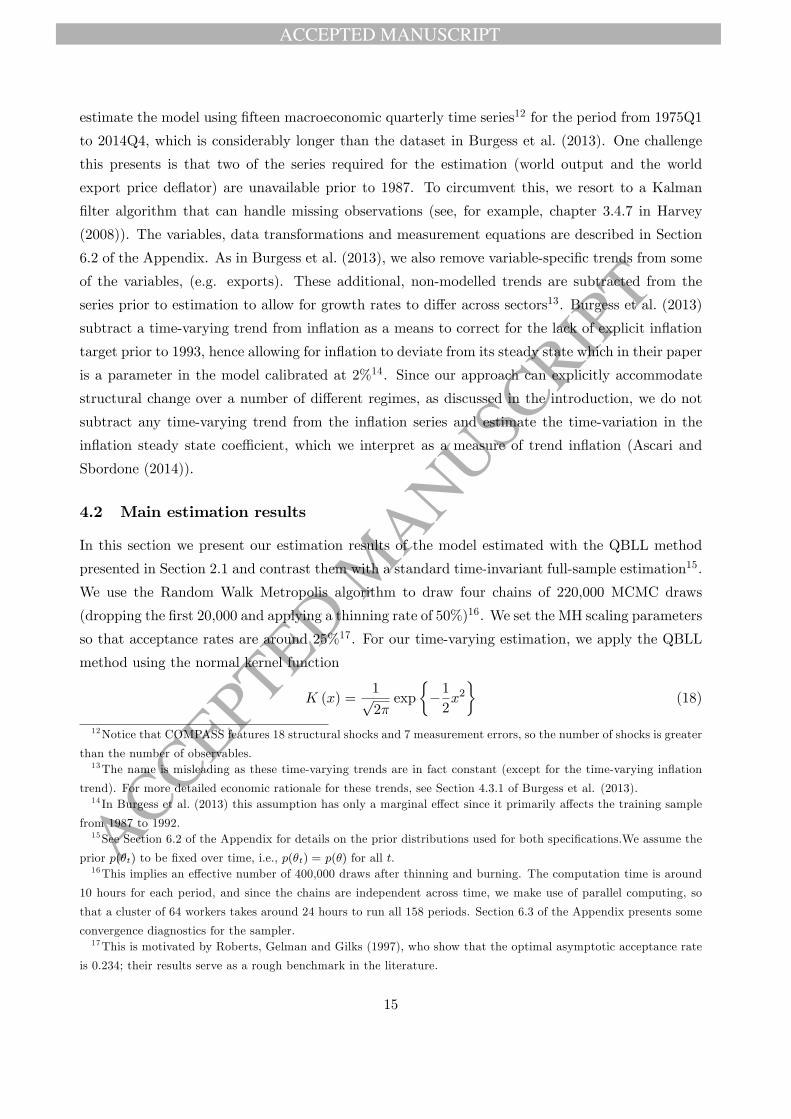
The first point worth highlighting relates to monetary policy. Over time, we can clearly see an in-
crease in the estimated responsiveness of interest rates to inflation, a reduction in the inflation
trend which has stabilised around its target level and a decline in the volatility of monetary policy
disturbances. All three are normally associated with more effective monetary policy as they are
synonymous with an economic environment characterised by low and stable inflation, well anchored
around its target18 (see DiCecio and Nelson (2009) for a detailed comparison of the US and UK
experiences). Moreover, our estimate of UK trend inflation is broadly in line with estimates for
18The period of very low and constant rates, at 50bps between 2009 and the end of our sample is reflected in a
marked increase in the interest rate smoothing coeffi cient as well as in moderate increase in the volatility of monetary
policy shocks, which increases from the estimate around 2000 but is still well below its constant parameter counterpart.
16
ACCEPTED MANUSCRIPT
ACCEPTED MANUSCRIP
T
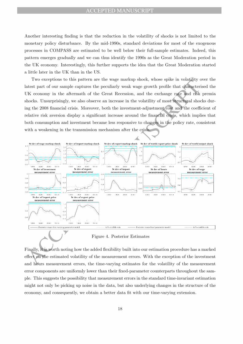
the US economy (surveyed in Ascari and Sbordone (2014)) with two differences: (i) the peak we
estimate in the 1970s is higher than in the US (about 8% in annual terms compared to 5% for the
baseline estimate in Ascari and Sbordone (2014)) consistent with evidence that the Great Inflation
was more severely felt in the UK, and (ii) the decline towards the 2% target takes longer to achieve,
implying that the Great Moderation started later than in the US19. Moreover, as demonstrated in
Section 4.6, allowing the trend inflation coeffi cient to vary has a significant effect on the both point
and density forecasts for CPI inflation, as well as import and export inflation, since the coeffi cient
appears in the intercept of the corresponding measurement equations.
Through the mid-1980s the policy responsiveness to inflation is close to unity while the esti-
mated annual inflation trend is as high as 8% percent. Over time monetary policy becomes more
responsive to inflation variations, the coeffi cient crossing the 1.5 value popularised by Taylor (1993)
around the time of the adoption of the inflation target (1992), while the inflation trend gradually
falls from about 3.5% down to its 2% target. The interest rate smoothing parameter, which enters
the model as a coeffi cient on the lagged policy rate in the Taylor rule, increases during the financial
crisis with values close to unity. As a result, during this period, the Taylor rule resembles a random
walk, which is a consequence of interest rates being close to the Zero Lower Bound.
Figure 3. Posterior Estimates
19Until 2003 the Bank of England’s inflation target was 2.5% on the RPI-X index.
17
ACCEPTED MANUSCRIPT
ACCEPTED MANUSCRIP
T
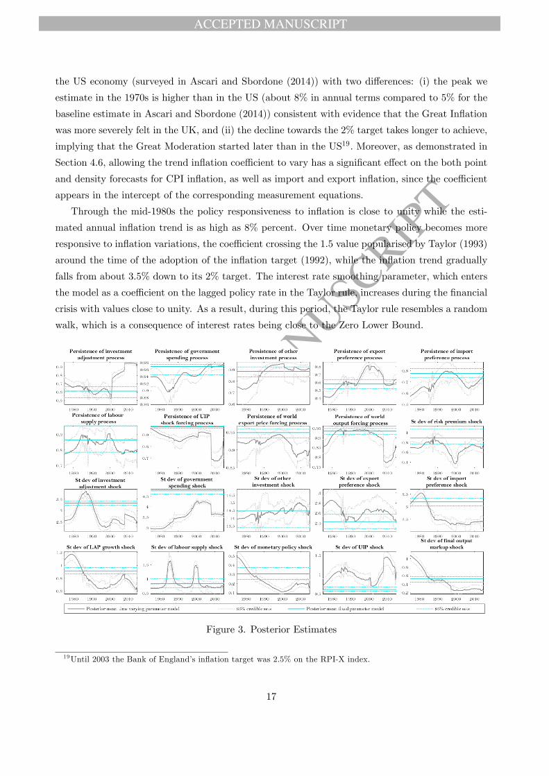
Another interesting finding is that the reduction in the volatility of shocks is not limited to the
monetary policy disturbance. By the mid-1990s, standard deviations for most of the exogenous
processes in COMPASS are estimated to be well below their full-sample estimates. Indeed, this
pattern emerges gradually and we can thus identify the 1990s as the Great Moderation period in
the UK economy. Interestingly, this further supports the idea that the Great Moderation started
a little later in the UK than in the US.
Two exceptions to this pattern are the wage markup shock, whose spike in volatility over the
latest part of our sample captures the peculiarly weak wage growth profile that characterised the
UK economy in the aftermath of the Great Recession, and the exchange rate and risk premia
shocks. Unsurprisingly, we also observe an increase in the volatility of most structural shocks dur-
ing the 2008 financial crisis. Moreover, both the investment-adjustment cost and the coeffi cient of
relative risk aversion display a significant increase around the financial crisis, which implies that
both consumption and investment became less responsive to changes in the policy rate, consistent
with a weakening in the transmission mechanism after the crisis.
Figure 4. Posterior Estimates
Finally, it is worth noting how the added flexibility built into our estimation procedure has a marked
effect on the estimated volatility of the measurement errors. With the exception of the investment
and hours measurement errors, the time-varying estimates for the volatility of the measurement
error components are uniformly lower than their fixed-parameter counterparts throughout the sam-
ple. This suggests the possibility that measurement errors in the standard time-invariant estimation
might not only be picking up noise in the data, but also underlying changes in the structure of the
economy, and consequently, we obtain a better data fit with our time-varying extension.
18
ACCEPTED MANUSCRIPT
ACCEPTED MANUSCRIP
T
Figure 5. Annual steady state inflation coeffi cient
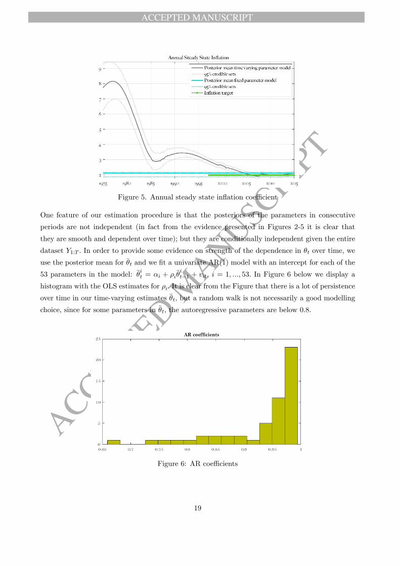
One feature of our estimation procedure is that the posteriors of the parameters in consecutive
periods are not independent (in fact from the evidence presented in Figures 2-5 it is clear that
they are smooth and dependent over time); but they are conditionally independent given the entire
dataset Y1:T . In order to provide some evidence on strength of the dependence in θt over time, we
use the posterior mean for θt and we fit a univariate AR(1) model with an intercept for each of the
53 parameters in the model: θit = αi + ρiθit−1 + vit, i = 1, ..., 53. In Figure 6 below we display a
histogram with the OLS estimates for ρi. It is clear from the Figure that there is a lot of persistence
over time in our time-varying estimates θt, but a random walk is not necessarily a good modelling
choice, since for some parameters in θt, the autoregressive parameters are below 0.8.
Figure 6: AR coeffi cients
19

ACCEPTED MANUSCRIPT
ACCEPTED MANUSCRIP
T
4.3 Metropolis-within-Gibbs results
In this section, we present the estimation results of the version of COMPASS with constant parame-
ters and time-varying volatility, estimated with the use of the Metropolis-within-Gibbs algorithm
from Section 2.2, based on two chains of 200,000 MCMC draws. Figures 7-10 display the estimated
parameters, comparing them with the estimates from our benchmark model and the standard fixed
parameter version. We draw several conclusions from these results. First, the estimated values for
the time-invariant parameters are very close to those from the standard fixed-parameter Bayesian
estimation. Second, the estimated time variation in the volatility of the structural shocks is also
very similar to the estimated volatility of our main model in Section 4.2. Third, the estimated
volatilities of the measurement errors increase once we treat the model parameters as constant.
We take this as evidence that the model fit of the version with changing volatility and constant
parameters is not as good as that of our benchmark model, resulting in larger measurement errors
(which absorb any discrepancies between the model and the data). Moreover, once we compare
the forecasting performance of the Metropolis-within-Gibbs version of the model in the forecasting
exercise in Section 4.6, we find that the resulting RMSFEs and LPSs are not better than the main
version of our model, which is further evidence that keeping the parameters constant delivers not
only worse in-sample fit but also worse out-of-sample performance.
Figure 7. MH-Gibbs algorithm parameter estimates
20

ACCEPTED MANUSCRIPT
ACCEPTED MANUSCRIP
T
Figure 8. MH-Gibbs algorithm parameter estimates
Figure 9. MH-Gibbs algorithm estimated time-varying structural shocks’volatilities
21

ACCEPTED MANUSCRIPT
ACCEPTED MANUSCRIP
T
Figure 10. MH-Gibbs algorithm estimated time-varying measurement errors’volatilities
4.4 Time-variation in the monetary transmission mechanism
We use the estimated time-varying parameters of our benchmark results in Section 4.2 to study
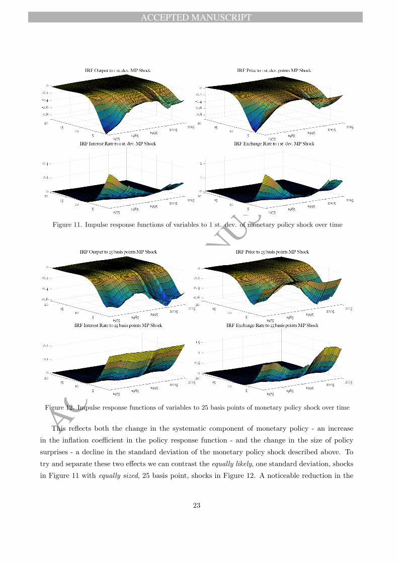
changes in the monetary transmission mechanism over time. Figures 11 and 12 display the impulse
responses for output, prices, the nominal interest rate and the exchange rate to a monetary policy
shock in each quarter of the estimation sample. Figure 11 displays responses to a one standard
deviation shock and captures the effect of the policy shock on the variables of interest, while also
taking into account the changing size of the shock. Responses of output and inflation to monetary
surprises are estimated to have been as much as four times as large in the 1970s than around
the turn of century. Indeed, these results are consistent with evidence presented in Boivin and
Giannoni (2006) for the U.S., who interpret the decreased responsiveness of inflation and output
to a monetary policy shock after the 1980s as a result of the monetary authority becoming more
effective and systematically more responsive in managing economic fluctuations.
22
ACCEPTED MANUSCRIPT
ACCEPTED MANUSCRIP
T
Figure 11. Impulse response functions of variables to 1 st. dev. of monetary policy shock over time
Figure 12. Impulse response functions of variables to 25 basis points of monetary policy shock over time
This reflects both the change in the systematic component of monetary policy - an increase
in the inflation coeffi cient in the policy response function - and the change in the size of policy
surprises - a decline in the standard deviation of the monetary policy shock described above. To
try and separate these two effects we can contrast the equally likely, one standard deviation, shocks
in Figure 11 with equally sized, 25 basis point, shocks in Figure 12. A noticeable reduction in the
23
ACCEPTED MANUSCRIPT
ACCEPTED MANUSCRIP
T
effects of a surprise 25 basis-point increase in the policy rate on output, the exchange rate and
inflation between the 1970s and the 1990s still emerges. Yet, the responses of output, the exchange
rate and, most notably, inflation show an increase over the most recent period despite the fact that
the estimation results suggest that consumption and investment have become less responsive to
interest rates. This reflects the marked increase in the policy rule smoothing coeffi cient (from a
value of about 0.75 in the 90s to above 0.9 in the latter part of our sample), which directly increases
the persistence of the interest rate. This is in turn partly a consequence of the policy rate having
been at, or close to, its effective lower bound since 2009.
4.5 Time-variation in variance decompositions
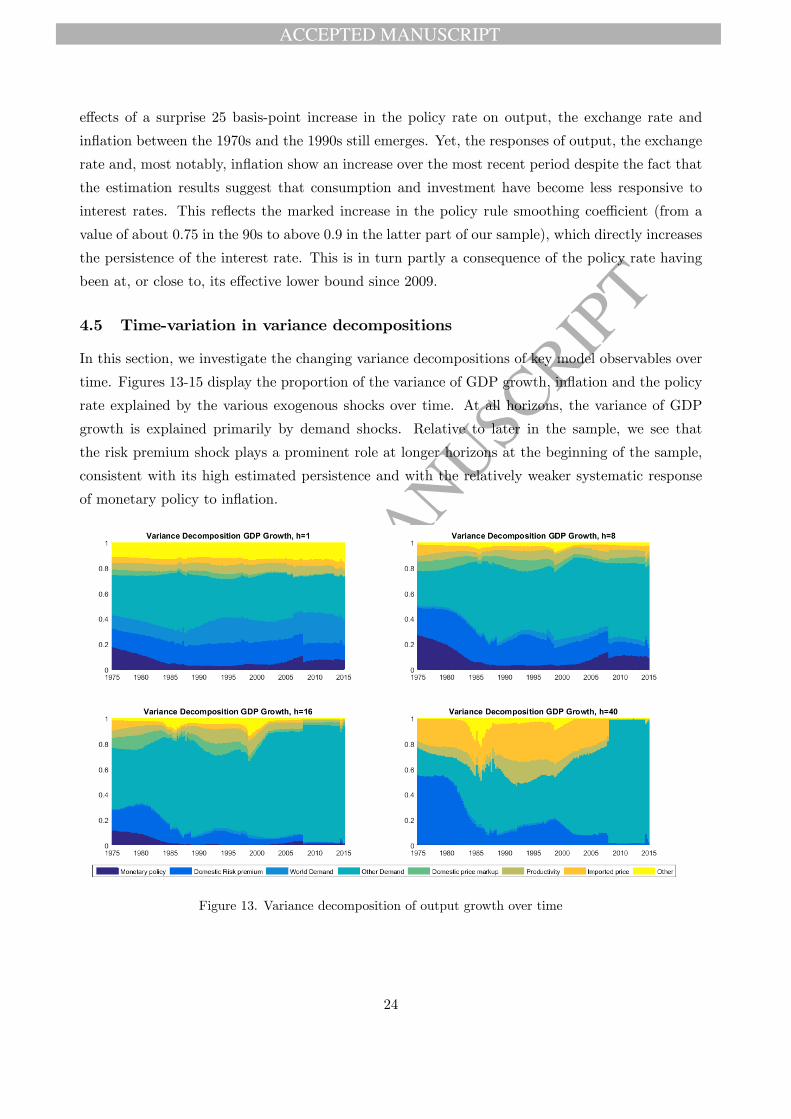
In this section, we investigate the changing variance decompositions of key model observables over
time. Figures 13-15 display the proportion of the variance of GDP growth, inflation and the policy
rate explained by the various exogenous shocks over time. At all horizons, the variance of GDP
growth is explained primarily by demand shocks. Relative to later in the sample, we see that
the risk premium shock plays a prominent role at longer horizons at the beginning of the sample,
consistent with its high estimated persistence and with the relatively weaker systematic response
of monetary policy to inflation.
Figure 13. Variance decomposition of output growth over time
24

ACCEPTED MANUSCRIPT
ACCEPTED MANUSCRIP
T
Figure 14. Variance decomposition of inflation over time
Figure 15. Variance decomposition of policy rate over time
Inflation’s variation is absorbed almost entirely by the variance of domestic mark up shocks at
25

ACCEPTED MANUSCRIPT
ACCEPTED MANUSCRIP
T
one quarter ahead, while at two and four years, we observe that the monetary policy shock also
has an effect, especially during the 1970s, early 1980s and the recent financial crisis, while the con-
tribution of risk premia is roughly constant and particularly marked at business cycle frequencies.
The pattern of the contribution of ‘imported inflation’to the overall variation in headline inflation
is particularly interesting. At long horizons, up to three quarters of inflation was explained by for-
eign factors in the 1970s, consistent with the widely-documented effects that oil prices had on UK
inflation at that time. Regarding the variance of the policy rate, it is interesting to note how the
overwhelming influence of monetary policy shocks in explaining its variation diminishes at longer
horizons while risk premia and other demand shocks take on a much more prominent role, just as
expected20.
4.6 Forecasting
In this section, we evaluate the relative forecasting performance of our time-varying parame-
ter COMPASS (TVP-COMPASS) model. In addition, we compare the forecasting record of
COMPASS against the fixed-parameter COMPASS (F-COMPASS) specification21, our Metropolis-
within-Gibbs version with constant parameters and time-varying volatility (MH-G-COMPASS),
an autoregressive model of order one with an intercept (AR(1)), a random walk model (RW), a
Bayesian VAR (BVAR)22, and a stochastic volatility VAR modelled as in Cogley and Sargent (2005)
and estimated with the Metropolis step of Jacquier, Polson and Rossi (1994) on three observables
(output growth, inflation and interest rates). We measure accuracy of point forecasts using the
root mean squared forecast error (RMSFE). The accuracy of density forecasts is measured by log
predictive scores (LPS). We compute the LPS with the help of a nonparametric estimator to smooth
the draws from the predictive density obtained for each forecast and horizon. For the AR(1) and
RW models we make use of wild bootstrap to approximate the predictive density. We test whether
the various models are statistically more accurate than our benchmark TVP-COMPASS with the
Diebold and Mariano (1995) statistic computed with the Newey-West estimator to obtain standard
errors. We provide the results of the Diebold-Mariano two-sided test for the RMSFEs and LPSs.
In addition, we also informally assess the density forecast performance of the models by plotting
the probability integral transformation (PIT) computed as the cumulative density function of the
nonparametric estimator for the predictive density at the ex-post realised value of the target variable
obtained for each forecast and horizon (Figure 16).
20Shocks to import prices also play an important role in the early part of our sample via the variation they induce
inflation.21See Fawcett, Koerber, Masolo and Waldron (2015) for further evaluation of the forecast performance of a fixed
parameter version of COMPASS against statistical and judgmental benchmarks.22The specification presented below is a BVAR(1) on all observables with Minnesota priors with overall shrinkage
0.1. We tried several other specifications in terms of lag length and overall shrinkage and found similar results.
26

ACCEPTED MANUSCRIPT
ACCEPTED MANUSCRIP
T
Table 1 presents the absolute performance of our time-varying parameter TVP-COMPASS
model (in RMSFEs) and the relative performance of the alternative models over different horizons
(numbers greater than one imply superior performance of the TVP-COMPASS relative to the al-
ternatives). One, two and three stars indicate that we reject the null of equal accuracy in favour
of the better performing model at significance levels of 10%, 5% and 1% respectively. From Table
1, it is clear that the time-varying specification of COMPASS can deliver better point forecasts for
most variables and horizons that the standard fixed parameter version of the model. The gains
over F-COMPASS for inflation forecast accuracy are nearly 40% at short horizons. In fact, we sta-
tistically outperfom all alternative models for inflation. This better inflation forecast performance
can be attributed to the considerable time-variation uncovered in the inflation trend, and the TVP-
COMPASS is the only included model that allows for changes in the long-run means of the series.
Our model also performs well against all alternatives for other variables such as exchange rates,
output, wage and consumption growth.
RMSFEs Forecast Origins: 1985Q1-2012Q4
horizon INFL Y INT C I EXCH IM INFL EX INFL W INFL H
1 0.37 0.85 0.20 0.77 6.19 3.57 1.97 2.94 0.94 0.95TVP- 2 0.40 0.70 0.35 0.76 5.43 3.65 2.19 2.59 0.98 0.67
COMPASS 4 0.44 0.65 0.56 0.83 5.40 3.66 2.00 2.16 0.91 0.608 0.48 0.70 0.83 0.79 5.69 3.47 1.93 1.88 0.93 0.651 1.63* 1.06 1.04 1.06 0.96* 1.03 1.24* 1.04 1.07* 1.05
F- 2 1.66* 1.00 1.09* 1.25* 0.97 1.01 1.23* 1.12* 1.09* 1.02COMPASS 4 1.35* 0.98 1.18* 1.20* 0.98 0.99 1.16* 1.14 1.04 1.16
8 0.98 0.92 1.17* 1.03 0.90 1.00 1.04 1.04 0.91* 1.021 1.37* 1.04 1.08* 0.96 0.92 1.10* 1.36* 0.86* 1.31* 1.05
MH-G IBBS 2 1.58* 0.99 1.15* 1.02 0.95 1.06* 1.22* 0.81* 1.39* 1.05COMPASS 4 1.64* 0.96 1.27* 1.06 0.94 1.03 1.08* 0.95 1.29* 1.12
8 1.36* 0.90 1.36* 0.99 0.84* 1.01 0.98 1.08* 1.04 1.021 1.18 0.80* 1.28* 1.08 1.12 1.55* 1.23* 0.82* 0.99 0.67*
RANDOM 2 1.18 1.12 0.97 1.17* 1.22 1.37* 1.13 0.98 0.99 1.04WALK 4 1.33* 1.38* 0.86 1.16 1.31 1.48* 1.36* 1.26* 1.00 1.29*
8 1.81* 1.41* 0.82 1.34* 1.26 1.56* 1.30* 1.35* 1.10 1.31*1 1.22* 0.75* 0.80* 1.08 0.97 1.04 0.93 0.68* 1.08 0.64*
AR(1) 2 1.39* 0.93 0.79* 1.07 0.97 1.01 0.91* 0.77* 0.95 0.81*4 1.64* 1.02 0.78* 0.99 0.95 1.00 0.96 0.93 1.23* 1.008 1.75* 0.94 0.78 1.03 0.90 1.02* 1.00 1.00 1.40* 1.091 1.48* 0.92 0.96 1.19* 0.95 1.21* 0.92 0.63* 0.94 0.54*
BVAR 2 1.25* 1.05 0.88 1.17* 0.97 1.09* 0.97 0.78* 0.88* 0.80*4 1.30* 1.19* 0.85 1.09 1.01 1.03 0.93 0.90 1.07 1.058 1.39* 1.03 0.92 1.09 0.94 1.02 0.94 0.96 1.20 1.041 1.22* 1.08* 0.79*
SV-BVAR 2 1.24* 1.88* 0.78*4 1.36* 1.21 0.75*8 1.47* 0.87 0.72*
Table 1. RMSFEs. The figures under TVP-COMPASS are absolute RMSFEs, computed as the mean of the predictive density,
the numbers under the remaining models are ratios over our benchmark time—varying parameter COMPASS model; ’*’, ’**’
and ’***’ indicate rejection of the null of equal performance against the two-sided alternative at 10%, 5% and 1%
significance level respectively, using a Diebold - Mariano test.
27

ACCEPTED MANUSCRIPT
ACCEPTED MANUSCRIP
T
Log Predictive Scores Forecast Origins: 1985Q1-2012Q4
horizon INFL Y INT C I EXCH IM INFL EX INFL W INFL H
1 -0.44 -1.32 0.04 -1.28 -3.15 -2.67 -2.28 -2.48 -1.35 -1.50TVP- 2 -0.53 -1.27 -0.75 -1.26 -2.93 -2.78 -2.44 -2.42 -1.40 -1.45
COM 4 -0.70 -1.28 -1.60 -1.33 -2.93 -2.76 -2.22 -2.34 -1.31 -1.458 -0.78 -1.31 -2.56 -1.30 -3.04 -2.72 -2.18 -2.32 -1.30 -1.481 -0.53*** -0.29*** -0.05 -0.32*** 0.07 -0.14** -0.07 -0.18*** -0.11** -0.28***
F- 2 -0.53*** -0.32*** 0.22 -0.40*** -0.07 0.00 -0.03 -0.23*** -0.13** -0.33***COM 4 -0.38** -0.32*** 0.29 -0.36*** -0.11** -0.02 -0.02 -0.28*** -0.20*** -0.35***
8 -0.28 -0.33*** 0.71 -0.39*** -0.02 -0.08 0.06 -0.27*** -0.18* -0.35***1 -0.26** -0.03 0.01 -0.01 0.11 -0.10* -0.35*** 0.02 -0.21** 0.02
MH-G 2 -0.51*** 0.04 -0.23** -0.07** 0.02 0.03 -0.14** -0.01 -0.31*** 0.06***COM 4 -0.52** 0.06*** -0.90*** -0.08 0.01 0.01 0.00 -0.11*** -0.27*** 0.05**
8 -0.29 0.07** -1.46*** -0.09*** 0.17 0.00 0.11 -0.13*** -0.18* 0.06**1 -0.19 0.12 -0.14 -0.07 -0.16 -0.46*** -0.04 -0.44* -0.06 -0.29
RW 2 -0.35** -0.20*** 0.49 -0.38*** -0.32*** -0.33* 0.00 -0.15 -0.01 0.224 -0.59*** -0.52*** 0.94* -0.68*** -0.57*** -0.62*** -0.49*** -0.22** -0.32*** 0.178 -0.97*** -0.85*** 1.56 -1.12*** -0.83*** -0.94*** -0.83*** -0.39*** -0.66*** -0.081 -0.23 0.40*** 0.52*** -0.01 0.12 -0.10 0.19** 0.23** -0.08 0.27
AR(1) 2 -0.41** 0.37*** 0.74** -0.02 -0.03 0.09 0.29*** 0.16 0.00 0.55***4 -0.50** 0.37*** 1.05** 0.07 -0.01 0.09 0.08 0.17 -0.27*** 0.48***8 -0.62** 0.44*** 1.53 0.07 0.08 0.05 0.03 0.27*** -0.53*** 0.291 -0.39*** 0.14** 0.20 -0.09 0.10 -0.18*** 0.31*** 0.33** 0.05 0.53**
BVAR 2 -0.33** 0.11 0.52 -0.12** -0.06 0.00 0.27** 0.21 0.14* 0.45*4 -0.35* -0.02 0.90* -0.09 -0.11* -0.02 0.09 0.19* -0.14 0.38**8 -0.43** 0.08 1.37 -0.14** -0.03 -0.03 0.05 0.28*** -0.30** 0.45***1 -0.10 -0.96*** 0.62***
SV- 2 -0.15 -0.33 0.85***BVAR 4 -0.13 0.40 1.03***
8 -0.22 1.39 1.49**
Table 2: Log Predictive Scores. The figures under TVP-COMPASS are absolute log predictive scores, computed as the log of
the predictive density evaluated at the ex-post realised observation, the figures under the remaining models are differences of log
scores over our benchmark time—varying parameter COMPASS model; ’*’, ’**’and ’***’indicate rejection of the null of equal
performance against the two-sided alternative at 10%, 5% and 1% significance level respectively, using a Diebold-Mariano test.
Table 2 assesses the quality of the density forecasts measured by LPS of the predictive density. The
table displays absolute LPS for the benchmark TVP-COMPASS model and differences in logscores
over the alternative models, so numbers greater smaller than zero imply superior performance of
the benchmark model. It is evident from Table 2 that allowing for time-variation in the parameters
of COMPASS delivers large and statistically significant improvements over the constant-parameter
model in the density forecasts for almost all variables and all horizons. This is likely to be a conse-
quence of the ability of the TVP model to capture changes in the volatility of the shocks. However,
allowing for time variation in the deep parameters is important too, since ‘switching’the variation
off with the use of our MH-G COMPASS does not deliver density forecast improvements alone,
partly as the predictive density is not entered well, which is evident from the worse point forecast
performance of the MH-G model. TVP-COMPASS also performs well in terms of density forecasts
compared to reduced-form models.
28

ACCEPTED MANUSCRIPT
ACCEPTED MANUSCRIP
T
Figure 16. Probability Integral Transformations
Another way of assessing density forecast performance of the models is by looking at the probability
integral transformation (PITs) in Figure 16, computed as the CDF of the predictive density of the
different models evaluated at the ex-post realised observation. For a well-calibrated density forecast
and a long enough sample, the out-turns in all parts of the distribution at all frequencies should
match the relevant probabilities, implying uniform PITs. The one-step ahead23 PITs in Figure 16
for selected variables reveal that none of our selection of models is very close to delivering a uniform
CDF. However, the TVP-COMPASS model is closer to uniform than the F-COMPASS variant, sug-
gesting that allowing for time-variation improves forecast density accuracy at the one-step ahead
horizon at least to some degree.
In summary, we find that by allowing the parameters of COMPASS to vary, we are able to
outperform the constant parameter COMPASS as well as the version with changing volatility,
both in terms of point and density forecasts for most variables and horizons. While in some cases
reduced-form models perform better, it is remarkable how a large structural model (designed for
policy analysis and not purely geared towards forecast accuracy) compares.
23For the sake of brevity, we report the one step ahead PITs. The results for other horizons reveal similar pattern.
29

ACCEPTED MANUSCRIPT
ACCEPTED MANUSCRIP
T
5 Conclusion
Standard Bayesian estimation of DSGE models relies on the assumption that the models’parame-
ters are time-invariant. Given that the UK economy has undergone substantial structural changes
over recent decades, not least those associated with changes in monetary regime, the constant-
parameter assumption is likely to be invalid except in very short sub-samples.
To address this shortcoming, in this paper we apply a quasi-Bayesian procedure developed by
Galvão et al. (2019) to the open economy DSGE model of the UK developed by Burgess et al.
(2013). Relative to Burgess et al. (2013), we extend the estimation sample to cover the period
between 1975 and 2014, by virtue of our time-varying estimation approach and a modified Kalman
filter that accommodates missing observations.
Our estimation detects clear signs of variation in the parameter estimates. Most notably, it
highlights the transition to a monetary policy regime characterised by long-term inflation expecta-
tions anchored at the target, an increased responsiveness of policy rates to inflation and a reduction
in the importance of the non-systematic component of monetary policy; all of which are associated
with more effective monetary policy.
Moreover, in our forecasting exercise we demonstrate that allowing for time-variation improves
both point and density forecast performance in a statistically significant way for most variables and
horizons. This is an important result since forecasting is one of the main uses of COMPASS in the
Bank of England.
ReferencesAdolfson, M., Andersson, M., Linde, J., Villani, M. and Vredin, A. (2007). Modern forecasting models in action: Improving
macroeconomic analyses at Central Banks, International Journal of Central Banking 3(4): 111—144.
Ascari, G. and Sbordone, A. M. (2014). The macroeconomics of trend inflation., Journal of Economic Literature 52(3): 679 —
739.
Benati, L. and Surico, P. (2009). VAR analysis and the Great Moderation, American Economic Review 99(4): 1636—1652.
Bianchi, F. (2013). Regime Switches, Agents’ Beliefs, and Post-World War II U.S. Macroeconomic Dynamics, Review of
Economic Studies 80: 463—490.
Boivin, J. and Giannoni, M. (2006). Has monetary policy become more effective?, Review of Economics and Statistics
88(3): 445—462.
Burgess, S., Fernandez-Corugedo, E., Groth, C., Harrison, R., Monti, F., Theodoridis, K. and Waldron, M. (2013). The Bank
of England’s forecasting platform: COMPASS, MAPS, EASE and the suite of models, Bank of England Working Paper
Series, No471 .
Canova, F. (2006). Monetary policy and the evolution of the US economy, CEPR Discussion Papers 5467 .
Canova, F. and Gambetti, L. (2009). Structural changes in the US economy: Is there a role for monetary policy, Journal of
Economic Dynamics and Control 33(2): 477—490.
30

ACCEPTED MANUSCRIPT
ACCEPTED MANUSCRIP
T
Canova, F. and Sala, L. (2009). Back to square one: Identifcation issues in DSGE models, Journal of Monetary Economics
56(4): 431—449.
Carter, C. K. and Kohn, R. (1994). On Gibbs sampling for state space models, Biometrica 81: 541—553.
Castelnuovo, E. (2012). Estimating the evolution of money’s role in the U.S. monetary business cycle, Journal of Money, Credit
and Banking 44(1): 23—52.
Chib, S. and Ramamurthy, S. (2010). Tailored randomized block mcmc methods with application to dsge models, Journal of
Econometrics 155(1): 19—38.
Christiano, L., Eichenbaum, M. and Evans, C. (2005). Nominal rigidities and the dynamic effects of a shock to monetary policy,
Journal of Political Economy 113(1): 1—45.
Cogley, T. and Sargent, T. J. (2002). Evolving post-World War II U.S. inflation dynamics, in B. S. Bernanke and K. Rogoff
(eds), NBER Macroeconomics Annual, MIT Press: Cambridge, pp. 331—88.
Cogley, T. and Sargent, T. J. (2005). Drifts and volatilities: Monetary policies and outcomes in the post World War II US,
Review of Economic Dynamics 8: 262—302.
Cogley, T. and Sbordone, A. M. (2008). Trend inflation, indexation, and inflation persistence in the new Keynesian Phillips
curve, American Economic Review 95(5): 2101—2126.
DiCecio, R. and Nelson, E. (2007). An estimated DSGE model for the United Kingdom, Working Papers 2007-006, Federal
Reserve Bank of St. Louis.
DiCecio, R. and Nelson, E. (2009). The Great Inflation in the United States and the United Kingdom: Reconciling Policy
Decisions and Data Outcomes, NBER Working Papers 14895, National Bureau of Economic Research, Inc.
Diebold, F. X. and Mariano, R. S. (1995). Comparing predictive accuracy, Journal of Business and Economic Statistics
13: 253—263.
Durbin, J. and Koopman, S. (2002). A simple and effi cient simulation smoother for state space time series analysis, Biometrika
89(3): 603—616.
Ellis, C., Mumtaz, H. and Zabczyk, P. (2014). What lies beneath? a time-varying favar model for the uk transmission
mechanism, The Economic Journal 124(576): 668—699.
Erceg, C. J., Henderson, D. W. and Levin, A. T. (2000). Optimal monetary policy with staggered wage and price contracts,
Journal of Monetary Economics 46(2): 281—313.
Fawcett, N., Koerber, L., Masolo, R. and Waldron, W. (2015). Evaluating UK point and density forecasts from an estimated
DSGE model: the role of off-model information over the financial crisis, Bank of England Working Paper Series, No538 .
Fernandez-Villaverde, J. and Rubio-Ramirez, J. F. (2008). How structural are the structural parameters, in K. R. D. Acemoglu
and M. Woodford (eds), NBER Macroeconomics Annual 2007, Vol. 22, Chicago: University of Chicago Press.
Foerster, A. T., Rubio-Ramirez, J. F., Waggoner, D. F. and Zha, T. A. (2014). Perturbation methods for Markov-switching
DSGE models, NBER Working Paper 258 .
Gali, J. and Gambetti, L. (2009). On the sources of the Great Moderation, American Economic Journal 1(1): 26—57.
Galvão, A. B., Giraitis, L., Kapetanios, G. and Petrova, K. (2016). A time varying DSGE model with financial frictions, Journal
of Empirical Finance 38: 690—716.
Galvão, A. B., Giraitis, L., Kapetanios, G. and Petrova, K. (2019). A quasi-Bayesian local likelihood method for medelling
parameter time variation in DSGE models, Working Paper .
31

ACCEPTED MANUSCRIPT
ACCEPTED MANUSCRIP
T
Giraitis, L., Kapetanios, G., Wetherilt, A. and Zikes, F. (2016). Estimating the dynamics and persistence of financial networks,
with an application to the Sterling money market, Journal of Applied Econometrics 31(1): 58—84.
Giraitis, L., Kapetanios, G. and Yates, T. (2014). Inference on stochastic time-varying coeffi cient models, Journal of Econo-
metrics 179(1): 46—65.
Harrison, R. and Oomen, O. (2010). Evaluating and estimating a DSGE model for the United Kingdom, Bank of England
working papers 380, Bank of England.
Harvey, C. A. (2008). Forecasting, Structural Time Series Models and the Kalman Filter, University of Cambridge Press.
Jacquier, E., Polson, N. G. and Rossi, P. (1994). Bayesian analysis of stochastic volatility models, Journal of Business and
Economic Statistics 12: 371—418.
Justiniano, A. and Primiceri, G. E. (2008). The time-varying volatility of macroeconomic fluctuations, American Economic
Review 98(3): 604—641.
Kydland, F. and Prescott, E. (1996). The computational experiment: an econometric tool, Journal of Economic Perspectives
10: 69—85.
Mumtaz, H. and Surico, P. (2009). Time-varying yield curve dynamics and monetary policy, Journal of Applied Econometrics
24(6): 895—913.
Petrova, K. (2019a). Quasi-bayesian estimation of time-varying volatility in dsge models, Journal of Time Series Analysis
40(1): 151—157.
Petrova, K. (2019b). A quasi-bayesian local likelihood approach to time varying parameter VAR models, Journal of Economet-
rics Forthcoming.
Primiceri, G. (2005). Time-varying structural vector autoregressions and monetary policy, Review of Economic Studies
72(3): 821—852.
Roberts, G., Gelman, A. and Gilks, W. (1997). Weak convergence and optimal scaling of random walk metropolis algorithms,
The Annals of Applied Probability 7(1): 110—120.
Rotemberg, J. (1982). Monopolistic price adjustment and aggregate output, Review of Economic Studies 49(4): 517—531.
Schmitt-Grohe, S. and Uribe, M. (2003). Closing small open economy models, Journal of International Economics 61(1): 163—
185.
Schorfheide, F. (2005). Learning and monetary policy shifts, Review of Economic Dynamics 8(2): 392—419.
Smets, F. and Wouters, R. (2007). Shocks and frictions in US business cycles: A Bayesian DSGE approach, American Economic
Review 97(3): 586—606.
6 Appendix
6.1 Algorithm for predictive density
The algorithm to compute the predictive density p(yT+h|yT ) h steps ahead consists of the following
steps:
Step 1. Using the saved draws from the quasi-posterior at the end of the sample p(θT |yT ),
for every draw i = 1, .., nsim, apply the Kalman filter to compute the moments of the unobserved
variables at T using the density p(xT |θiT , yT ).
32
ACCEPTED MANUSCRIPT
ACCEPTED MANUSCRIP
T
Step 2. Draw a sequence of shocks viT+1:T+h and measurement errors from N (0, Q(θiT )) and
N (0, R(θiT )) respectively, where Q(θiT ) and R(θiT ) are draws from the estimated quasi-posterior
distribution of the diagonal covariance matrices of the shocks and measurement errors at T . For
each draw i from p(θT |yT ) and p(xT |θiT , yT ), use the state equation to obtain forecasts for the
unobserved variables
xiT+1:T+h = F (θiT )xiT :T+h−1 +G(θiT )viT+1:T+h.
Step 3. Use the forecast simulations for the latent variables xiT+1:T+h and the measurement
errors draw ϑiT+1:T+h in the measurement equation
yiT+1:T+h = K(θiT ) + Z(θiT )xiT+1:T+h + ϑiT+1:T+h.
Once the simulated forecasts yiT+1:T+h are obtained, they can be used to obtain numerical approx-
imations of moments, quantiles and densities of the forecasts. Point forecasts can be computed as
the mean of the predictive density of yiT+1:T+h for each forecasting horizon.
6.2 Priors and ObservablesParameter Description ValueωCZ Steady state share of consumption in final output 0.5031ωIZ Steady state share of business investment in final output 0.0845ωIOZ Steady state share of ‘other’investment in final output 0.0370ωGZ Steady state share of government spending in final output 0.1662ωXZ Steady state share of exports in final output 0.2092ωMZ Steady state share of imports in final output 0.2197ΓH Trend population growth 1.0020ΓZ Trend productivity growth 1.0070ΓI Trend investment growth relative to final output growth 1.0036ΓX Trend export growth relative to final output growth 1.0025ΓG Trend government spending growth relative to final output 0.9950β Household discount factor 0.9986ωLV Steady state labour share 0.6774ωV Z Steady state value added share 0.7599µZ Steady state final output price mark-up 1.0050δK Capital depreciation rate 0.0077ζωF Speed at which rest of the world inherits LAP shocks 0.9000βfactor ‘Over-discounting’factor 0.0100σµV Standard deviation of value added price mark-up shock 0.0500σTFP Standard deviation of TFP shock 0.0500ρTFP Persistence of TFP forcing process 0.9000ρLAP Persistence of LAP forcing process 0.0000
Table 3: Calibrated parameters
33

ACCEPTED MANUSCRIPT
ACCEPTED MANUSCRIP
T
PriorParameter Description Distribution Mean StdΠ∗ Inflation Target Normal 1.005 0.25θR Policy rule interest rate smoothing Beta 0.800 0.100θΠ Policy rule inflation response Normal 1.500 0.250θY Policy rule output gap response Beta 0.125 0.075φZ Final output price adjustment cost Gamma 7.000 2.000φV Value added price adjustment cost Gamma 7.000 2.000φM Import price adjustment cost Gamma 10.00 2.000φX Export price adjustment cost Gamma 10.00 2.000φW Nominal wage adjustment cost Gamma 14.00 2.000ξZ Indexation of final output prices Beta 0.25 0.075ξV Indexation of value added prices Beta 0.25 0.075ξM Indexation of import prices Beta 0.25 0.075ξX Indexation of export prices Beta 0.25 0.075ξW Indexation of nominal wages Beta 0.25 0.075ψC Habit formation parameter Beta 0.70 0.150ψI Investment adjustment cost Gamma 2.00 0.400εC Coeffi cient of relative risk aversion Gamma 1.50 0.200εL Labour supply elasticity Gamma 2.00 0.300εF Price elasticity world demand, UK exports Gamma 0.75 0.100ωo Share of optimising households Beta 0.70 0.050ρB Persistence of risk premium forcing process Beta 0.75 0.100ρI Persistence of investment adjustment shock Beta 0.75 0.100ρG Persistence of government spending shock Beta 0.90 0.050ρIO Persistence of other investment shock Beta 0.75 0.100ρκF Persistence of export preference shock Beta 0.75 0.100ρM Persistence of import preference shock Beta 0.75 0.100ρL Persistence of labour supply shock Beta 0.75 0.100
Table 4: PriorsPrior
Parameter Description Distribution Mean StdρBF Persistence of UIP shock Beta 0.75 0.10ρPXF Persistence of world export price shock Beta 0.90 0.05ρZF Persistence of world output shock Beta 0.90 0.05σB St dev of risk premium shock Gamma 0.50 0.20σI St dev of investment adjustment shock Gamma 1.90 0.20σG St dev of government spending shock Gamma 3.00 0.20σIO St dev of other investment shock Gamma 14.0 1.00σκF St dev of export preference shock Gamma 2.20 0.20σM St dev of import preference shock Gamma 2.20 0.20σLAP St dev of LAP growth shock Gamma 0.35 0.10σL St dev of labour supply shock Gamma 0.75 0.20σR St dev of monetary policy shock Gamma 0.10 0.10σBF St dev of UIP shock Gamma 0.65 0.20σµZ St dev of final output markup shock Gamma 0.10 0.10σµW St dev of wage markup shock Gamma 0.30 0.10σµM St dev of import markup shock Gamma 1.30 0.20σµX St dev of export markup shock Gamma 1.30 0.20σPXF St dev of world export price shock Gamma 1.60 0.20σZF St dev of world output shock Gamma 2.50 0.20σmei St dev of investment measurement error Gamma 0.35 0.10σmeX St dev of export measurement error Gamma 0.18 0.055σmeM St dev of import measurement error Gamma 0.18 0.055σmeL St dev of hours measurement error Gamma 0.045 0.013σmeW St dev of wage measurement error Gamma 0.125 0.0275σmePM St dev of import price measurement error Gamma 0.34 0.075σmePX St dev of export price measurement error Gamma 0.34 0.075
Table 5: Priors
34
ACCEPTED MANUSCRIPT
ACCEPTED MANUSCRIP
T
Variable Description Data transformation equation Measurement equation
gdpkp Real GDP dlngdpkpt ≡ 100∆ ln gdpkpt ∆vt + γZt + 100 ln
(ΓZΓH
(ΓX)− 1−αV
αV
)ckp Real cons. dlnckpt ≡ 100∆ ln ckpt ∆ct + γZt + 100 ln
(ΓZΓH
)ikkp Real inv. dlnikkpt ≡ 100∆ ln ikkpt ∆it + γZt + 100 ln
(ΓZΓHΓI
)+ σmeI meIt
gonskp Real spending dlngonskpt ≡ 100∆ ln gonskpt ∆gt + γZt + 100 ln(ΓZΓHΓG
)xkp Real exports dlnxkpt ≡ 100∆ ln xkpt − dlnxkpttt ∆xt + γZt + 100 ln
(ΓZΓHΓX
)+ σmeX meXt
mkp Real imports dlnmkpt ≡ 100∆ lnmkpt − dlnmkpttt ∆mt + γZt + 100 ln(ΓZΓHΓX
)+ σmeM meMt
pxdef Export deflator dlnpxdeft ≡ 100∆ ln pxdeft −Π∗,ttt −Πx,ttt ∆pEXt −∆qt + πZt + 100 ln Π∗
ΓX+ σmePXme
PXt
pmdef Import deflator dlnpmdeft ≡ 100∆ ln pmdeft −Π∗,ttt −Πm,ttt πMt + 100 ln Π∗
ΓX+ σmePMme
PMt
awe Nom. wage dlnawet ≡ ∆ ln awet −Π∗,ttt ∆wt + γZt + πZt + 100 ln(ΓZΠ∗
)+ σmeW meWt
cpisa SA CPI dlncpisat ≡ 100∆ ln cpisat −Π∗,ttt πCt + 100 ln Π∗
rga Bank Rate robst ≡ 100 ln(1 + rgat
100
) 14 −Π∗,ttt rt + 100 lnR
eer Sterling ERI dlneert ≡ 100∆ ln eert ∆qt − πZthrs Hours worked dlnhrst ≡ 100∆ ln hrst ∆lt + 100 ln ΓH + σmeL meLtyf World output dlnyft ≡ 100∆ ln yft − dlnyfttt ∆zFt + γZt + 100 ln
(ΓZΓH
)pxfdef World exp. def. dlnpxfdeft ≡ 100∆ ln pxfdeft −Πxf,tt
t ∆pXF
t + 100 ln Π∗
ΓX
Table 6: Observables, data transformation and measurement equations
6.3 Convergence Diagnostics
Figure 17: Ineffi ciency factors
In this section we provide some convergence diagnostics for the MCMC sampler. First we com-
pute ineffi ciency factors for chain c, period t, parameter i, given by τ t,c,i =∑∞
k=−∞ ρt,c,i,k =
1 + 2∑∞
k=1 ρt,c,i,k, where ρt,c,i,k is the autocorrelation function of each chain (τ t,c,i is approximated
numerically using correlogram and Parzen kernel). Ineffi ciency factors have the following interpre-
tation: in order to obtain 1,000 i.i.d. draws from the posterior, τ t,c,i×1,000 draws are required.
35
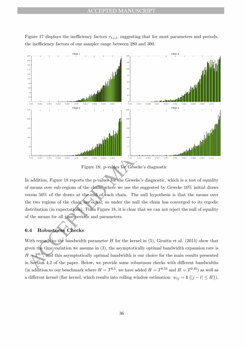
ACCEPTED MANUSCRIPT
ACCEPTED MANUSCRIP
T
Figure 17 displays the ineffi ciency factors τ t,c,i, suggesting that for most parameters and periods,
the ineffi ciency factors of our sampler range between 280 and 300.
Figure 18: p-values for Geweke’s diagnostic
In addition, Figure 18 reports the p-values for the Geweke’s diagnostic, which is a test of equality
of means over sub-regions of the chain; where we use the suggested by Geweke 10% initial draws
versus 50% of the draws at the end of each chain. The null hypothesis is that the means over
the two regions of the chain are equal; so under the null the chain has converged to its ergodic
distribution (in expectations). From Figure 18, it is clear that we can not reject the null of equality
of the means for all time periods and parameters.
6.4 Robustness Checks
With regards to the bandwidth parameter H for the kernel in (5), Giraitis et al. (2014) show that
given the time variation we assume in (3), the asymptotically optimal bandwidth expansion rate is
H = T 0.5, and this asymptotically optimal bandwidth is our choice for the main results presented
in Section 4.2 of the paper. Below, we provide some robustness checks with different bandwidths
(in addition to our benchmark where H = T 0.5, we have added H = T 0.55 and H = T 0.45) as well as
a different kernel (flat kernel, which results into rolling window estimation: wtj = 1 |j − t| ≤ H).
36

ACCEPTED MANUSCRIPT
ACCEPTED MANUSCRIP
T
Figure 18: Robustness: parameter estimates with different bandwidths
Figure 19: Robustness: parameter estimates with different bandwidths
37

ACCEPTED MANUSCRIPT
ACCEPTED MANUSCRIP
T
Figure 20: Robustness: parameter estimates with different bandwidths
Figure 21: Robustness: steady state inflation with different bandwidths
Figures 18-21 summarise the main findings from the robustness checks. As expected, larger band-
widths provide smoother estimates, but the patterns in the parameters over time are very similar,
and most of the time, these different bandwidth estimates are inside the 95% posterior bands of
our benchmark estimates. Note also that larger bandwidths imply larger effective sample size, and
so lesser effect of the prior on the estimates; while smaller bandwidths give greater weight on the
prior which can introduce some finite sample bias. Moreover, the estimates resulting from the
rolling window scheme are considerably more noisy, which is an unattractive feature which makes
the results hard to interpret and suggests that the use of exponential kernels is preferable.
38