Embed Size (px)
Citation preview
1
A THESIS SUBMITTED TO THE GRADUATE
SCHOOL OF APPLIED SCIENCES
OF
NEAR EAST UNIVERSITY
By
YASMINA F OMAR BADER
In Partial Fulfilment of the Requirements for
The Degree of Master of Science
in
Mathematics
NICOSIA, 2018
YA
SM
INA
F O
MA
R
BA
DE
R
FR
AC
TIO
NA
L C
AL
CU
LU
S A
ND
IT'S
AP
PL
ICA
TIO
NS
TO
FR
AC
TIO
NA
L D
IFF
ER
EN
TIA
L E
QU
AT
ION
S
NE
U
2018
2
FRACTIONAL CALCULUS AND IT'S
APPLICATIONS TO FRACTIONAL DIFFERENTIAL
EQUATIONS
A THESIS SUBMITTED TO THE GRADUATE
SCHOOL OF APPLIED SCIENCES
OF
NEAR EAST UNIVERSITY
By
YASMINA F OMAR BADER
In Partial Fulfilment of the Requirements for
The Degree of Master of Science
in
Mathematics
NICOSIA, 2018
3
Yasmina Bader: FRACTIONAL CALCULUS AND IT'S
APPLICATIONS TO FRACTIONAL DIFFERENTIAL EQUATIONS
Approval of Director of Graduate School of
Applied Sciences
Prof. Dr. Nadire ÇAVUŞ
Director
We certify that, this thesis is satisfactory for the award of the degree of Master of
Science in Mathematics
Examining Committee in Charge:
Prof. Dr. Allaberen Ashyralyev
Supervisor, Department of Mathematics,
Near East University
Assoc. Prof. Dr. Evren Hınçal Department of Mathematics, Near East
University
Assoc. Prof. Dr. Deniz Agirseven Department of Mathematics, Trakya
University
4
I hereby declare that all information in this document has been obtained and presented in
accordance with academic rules and ethical conduct. I also declare that, as required by
these rules and conduct, I have fully cited and referenced all material and results that are
not original to this work.
Name, last name: Yasmina Bader
Signature:
Date:

i
ACKNOWLEDGMENTS
I truly wish to express my heartfelt thanks to my supervisor Prof. Dr. Allaberen
Ashyralyev for his patience, support and professional guidance throughout this thesis
project. Without his encouragement and guidance the study would not have been
completed.
I use this medium to acknowledge the help, support and love of my husband Mustafa .
My special appreciation and thanks goes to my parents for their direct and indirect
motivation and supporting to complete my master degree.
Last but not the least; I would like to thank my colleagues, brothers, and sisters for
supporting me physically and spiritually throughout my life. May Allah reward them with
the best reward.

ii
To my parents
iii
ABSTRACT
In this thesis fractional calculus and its applications to stability for the fractional Basset
equation are studied. Most important properties of fractional order integrals and derivatives
are discussed. In applications, methods for the solutions of initial value problem for
fractional differential equations are considered. Stability of initial value problem is
illustrated with a special type of fractional differential equation.
( ) ( ) ( ) ( )
where and which is known as Basset equation.
Keywords: Fractional calculus; Fractional differential equations; Basset equation; Stability;
Numerical solution
iv
ÖZET
Bu tezde kesirli kalkülüs ve Basset denklemi için kararlılığa uygulamaları incelenmiştir.
Kesirli mertebeden integrallerin ve türevlerin en önemli özellikleri tartışılmştır.
Uygulamalarda, kesirli diferansiyel denklemler için başlangıç değer probleminin çözümleri
için yöntemler göz önüne alınmıştır. Başlangıç değer probleminin kararlılığı, ve
olarak üzere Basset denklemi olarak bilinir.
( ) ( ) ( ) ( )
özel bir kesirli diferansiyel denklem için gösterilmiştir.
Anahtar Kelimeler: Kesirli hesap; Kesirli diferansiyel denklemler; Baset denklemi;
Kararlılık; Sayısal çözüm
v
TABLE OF CONTENTS
ACKNOWLEDGMENTS ............................................................................................ I
ABSTRACT .................................................................................................................. III
ÖZET ............................................................................................................................ IV
TABLE OF CONTENTS ............................................................................................. V
CHAPTER 1: INTRODUCTION ............................................................................... 1
CHAPTER 2: RIEMANN – LIOUVILLE FRACTIONAL INTEGRAL
2.1 Auxiliary Lemma ...................................................................................................... 4
2.2 Riemann - Liouville Fractional Integral .................................................................. 5
CHAPTER 3: CAPUTO FRACTIONAL DIFFERENTIAL OPERATOR ........... 15
CHAPTER 4: RIEMANN-LIOUVILLE FRACTIONAL OPERATOR ............... 30
CHAPTER 5: FRACTIONAL ORDINARY DIFFERENTIAL EQUATIONS .... 38
CHAPTER 6: STABILITY OF DIFFERENTIAL AND DIFFERENCE
PROBLEMS
6.1 The stability of the initial-value problem for Basset equation ................................. 63
6.2 The stability of the difference scheme for the Basset equation ................................ 69
CHAPTER 7: CONCLUSIONS .................................................................................. 84
REFERENCES ............................................................................................................ 85
APPENDIX ................................................................................................................. 88
1
CHAPTER 1
INTRODUCTION
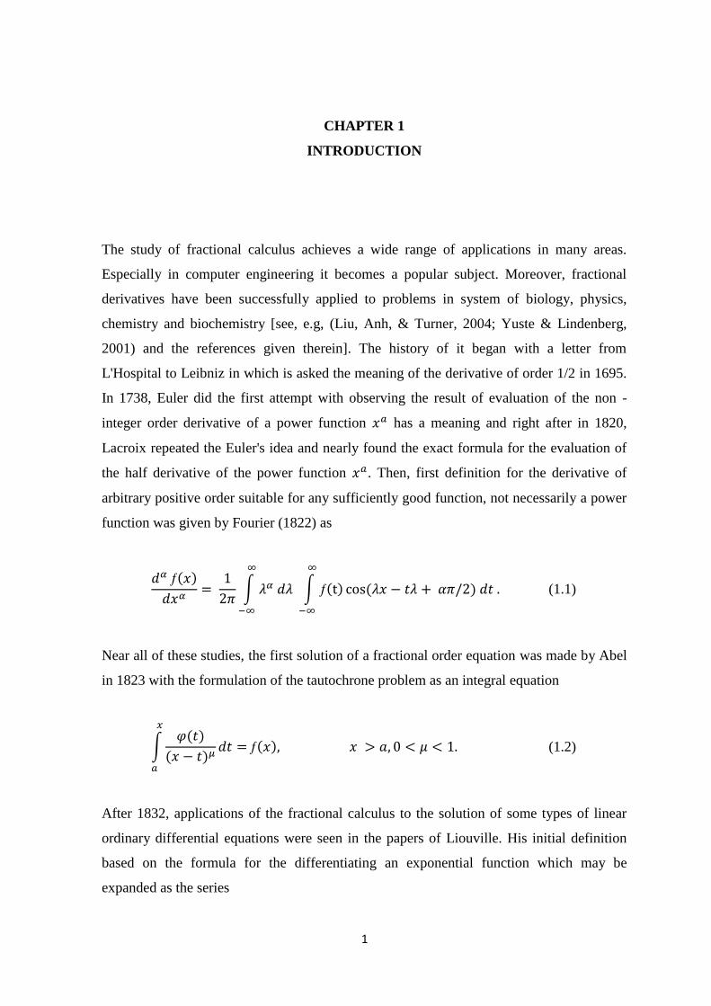
The study of fractional calculus achieves a wide range of applications in many areas.
Especially in computer engineering it becomes a popular subject. Moreover, fractional
derivatives have been successfully applied to problems in system of biology, physics,
chemistry and biochemistry [see, e.g, (Liu, Anh, & Turner, 2004; Yuste & Lindenberg,
2001) and the references given therein]. The history of it began with a letter from
L'Hospital to Leibniz in which is asked the meaning of the derivative of order 1/2 in 1695.
In 1738, Euler did the first attempt with observing the result of evaluation of the non -
integer order derivative of a power function has a meaning and right after in 1820,
Lacroix repeated the Euler's idea and nearly found the exact formula for the evaluation of
the half derivative of the power function . Then, first definition for the derivative of
arbitrary positive order suitable for any sufficiently good function, not necessarily a power
function was given by Fourier (1822) as
( )
∫ ∫ ( ) ( )
(1.1)
Near all of these studies, the first solution of a fractional order equation was made by Abel
in 1823 with the formulation of the tautochrone problem as an integral equation
∫ ( )
( )
( ) (1.2)
After 1832, applications of the fractional calculus to the solution of some types of linear
ordinary differential equations were seen in the papers of Liouville. His initial definition
based on the formula for the differentiating an exponential function which may be
expanded as the series
2
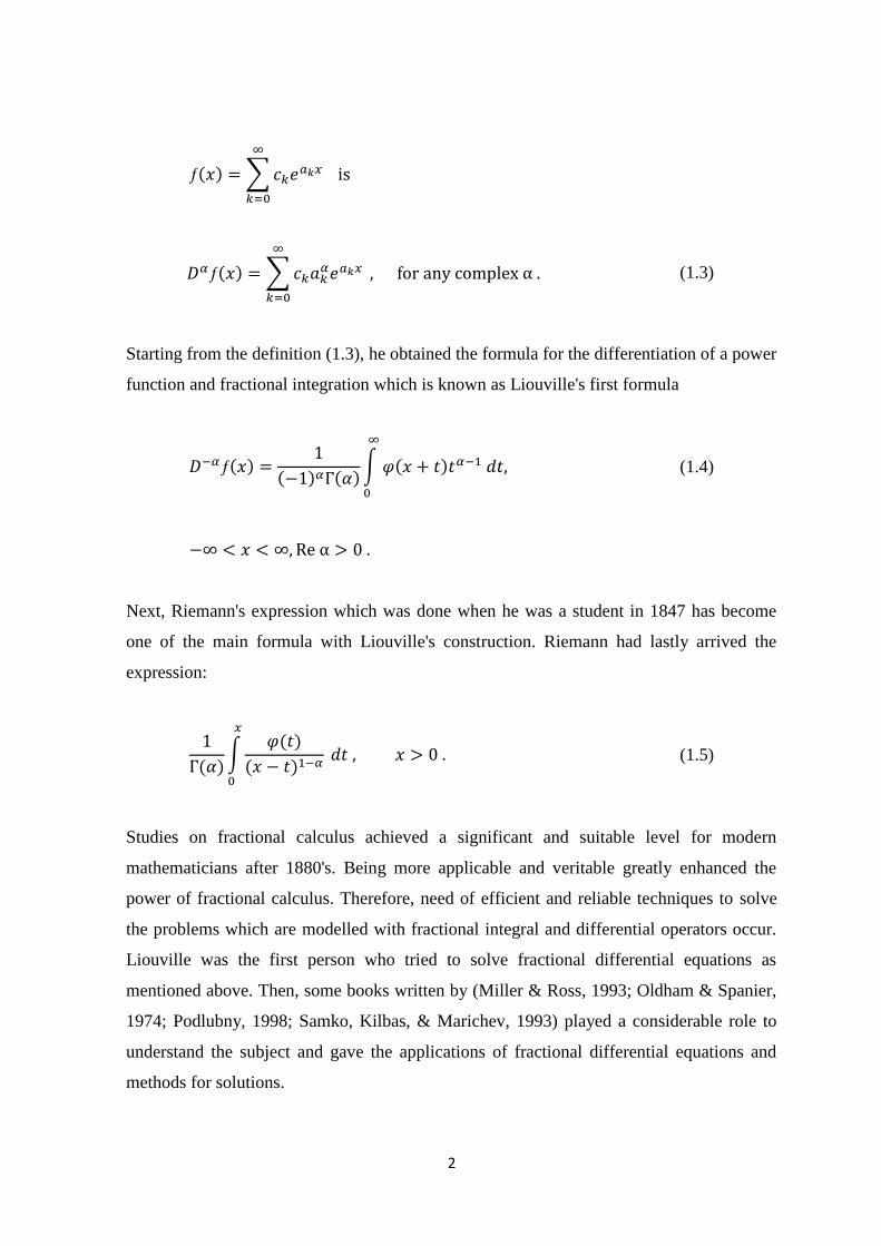
( ) ∑
( ) ∑
(1.3)
Starting from the definition (1.3), he obtained the formula for the differentiation of a power
function and fractional integration which is known as Liouville's first formula
( )
( ) ( )∫ ( )
(1.4)
Next, Riemann's expression which was done when he was a student in 1847 has become
one of the main formula with Liouville's construction. Riemann had lastly arrived the
expression:
( )∫
( )
( )
(1.5)
Studies on fractional calculus achieved a significant and suitable level for modern
mathematicians after 1880's. Being more applicable and veritable greatly enhanced the
power of fractional calculus. Therefore, need of efficient and reliable techniques to solve
the problems which are modelled with fractional integral and differential operators occur.
Liouville was the first person who tried to solve fractional differential equations as
mentioned above. Then, some books written by (Miller & Ross, 1993; Oldham & Spanier,
1974; Podlubny, 1998; Samko, Kilbas, & Marichev, 1993) played a considerable role to
understand the subject and gave the applications of fractional differential equations and
methods for solutions.
3
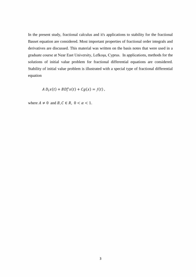
In the present study, fractional calculus and it's applications to stability for the fractional
Basset equation are considered. Most important properties of fractional order integrals and
derivatives are discussed. This material was written on the basis notes that were used in a
graduate course at Near East University, Lefkoşa, Cyprus. In applications, methods for the
solutions of initial value problem for fractional differential equations are considered.
Stability of initial value problem is illustrated with a special type of fractional differential
equation
( ) ( ) ( ) ( )
where and .
4
CHAPTER 2
RIEMANN – LIOUVILLE FRACTIONAL INTEGRAL
This chapter contain the definition and some properties of the Riemann-Liouville fractional
integrals.
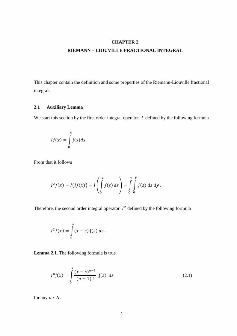
2.1 Auxiliary Lemma
We start this section by the first order integral operator I defined by the following formula
( ) ∫ ( )
From that it follows
( ) ( ( )) (∫ ( )
) ∫ ∫ ( )
Therefore, the second order integral operator defined by the following formula
( ) ∫( ) ( )
Lemma 2.1. The following formula is true
( ) ∫( )
( ) ( )
(2.1)
for any
5
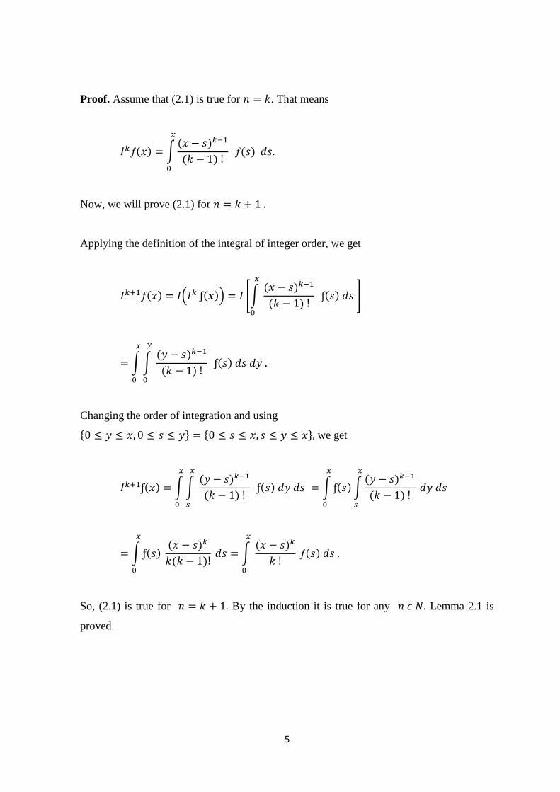
Proof. Assume that (2.1) is true for . That means
( ) ∫( )
( ) ( )
Now, we will prove (2.1) for
Applying the definition of the integral of integer order, we get
( ) . ( )/ [∫ ( )
( ) ( )
]
∫ ∫ ( )
( ) ( )
Changing the order of integration and using
* + * + we get
( ) ∫ ∫ ( )
( ) ( ) ∫ ( ) ∫
( )
( )
∫ ( ) ( )
( ) ∫
( )
( )
So, (2.1) is true for By the induction it is true for any Lemma 2.1 is
proved.
6
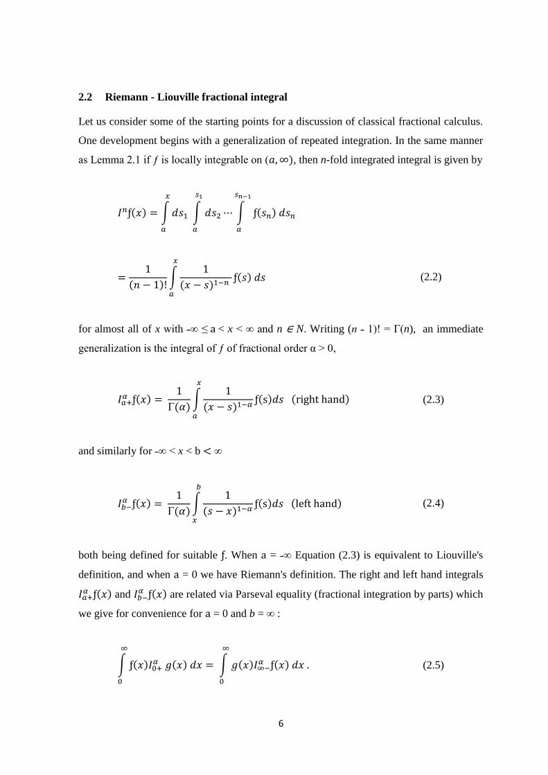
2.2 Riemann - Liouville fractional integral
Let us consider some of the starting points for a discussion of classical fractional calculus.
One development begins with a generalization of repeated integration. In the same manner
as Lemma 2.1 if is locally integrable on ( ), then n-fold integrated integral is given by
( ) ∫ ∫
∫ ( )
( ) ∫
( ) ( )
(2.2)
for almost all of x with ˗∞ ≤ < x < ∞ and n N. Writing (n ˗ 1)! = Г(n), an immediate
generalization is the integral of of fractional order α > 0,
( )
Г( )∫
( )
( ) ( ) (2.3)
and similarly for ˗∞ < x < b < ∞
( )
Г( )∫
( )
( ) ( ) (2.4)
both being defined for suitable . When = ˗∞ Equation (2.3) is equivalent to Liouville's
definition, and when = 0 we have Riemann's definition. The right and left hand integrals
( ) and
( ) are related via Parseval equality (fractional integration by parts) which
we give for convenience for = 0 and b = ∞ :
∫ ( ) ( ) ∫ ( )
( )
(2.5)
7
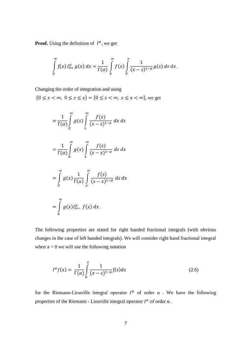
Proof. Using the definition of , we get
∫ ( )
( )
( ) ∫ ( ) ∫
( )
( )
Changing the order of integration and using
* + * +, we get
( )∫ ( )
∫ ( )
( )
( )∫ ( )
∫ ( )
( )
∫ ( )
( ) ∫
( )
( )
∫ ( )
( )
The following properties are stated for right handed fractional integrals (with obvious
changes in the case of left handed integrals). We will consider right hand fractional integral
when = 0 we will use the following notation
( )
Г( )∫
( )
( ) (2.6)
for the Riemann-Liouville integral operator of order α . We have the following
properties of the Riemann - Liouville integral operator of order α .
8
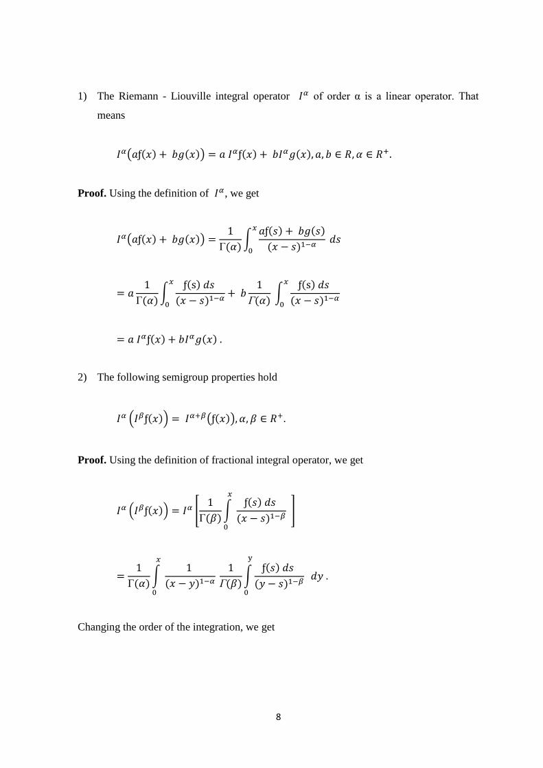
1) The Riemann - Liouville integral operator of order α is a linear operator. That
means
( ( ) ( )) ( ) ( )
Proof. Using the definition of , we get
( ( ) ( ))
Г( )∫
( ) ( )
( )
Г( )∫
( )
( )
( ) ∫
( )
( )
( ) ( )
2) The following semigroup properties hold
. ( )/ ( ( ))
Proof. Using the definition of fractional integral operator, we get
. ( )/ [
Г( )∫
( )
( )
]
Г( )∫
( )
( )∫
( )
( )
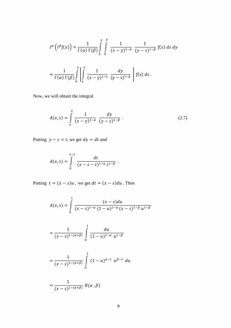
Changing the order of the integration, we get
9
. ( )/
Г( ) Г( )∫ ∫
( )
( ) ( )
Г( ) Г( )∫ [∫
( ) α
( )
] ( )
Now, we will obtain the integral
( ) ∫
( )
( )
(2.7)
Putting we get and
( ) ∫
( )
Putting ( ) we get ( ) Then
( ) ∫ ( )
( ) ( ) ( )
( ) ( ) ∫
( )
( ) ( ) ∫ ( )
( ) ( ) ( )
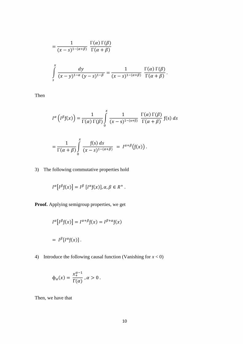
11
( ) ( ) Г( ) Г( )
Г( )
∫
( ) ( )
( ) ( ) Г( ) Г( )
Г( )
Then
. ( )/
Г( ) Г( )∫
( ) (α ) Г( ) Г( )
Г( ) ( )
Г( )∫
( )
( ) ( )
( ( ))
3) The following commutative properties hold
[ ( )] , ( )-
Proof. Applying semigroup properties, we get
[ ( )] ( ) ( )
, ( )-
4) Introduce the following causal function (Vanishing for x < 0)
( )
( )
Then, we have that
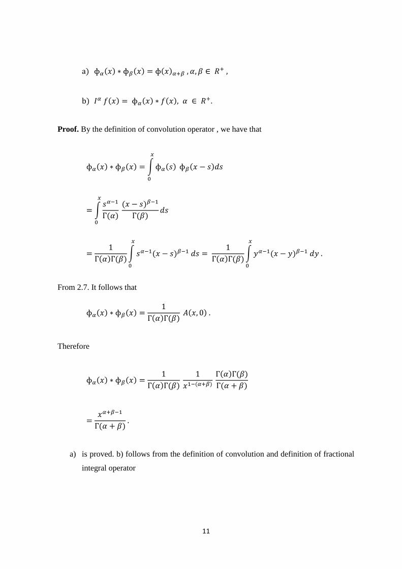
11
a) ( ) ( ) ( )
b) ( ) ( ) ( )
Proof. By the definition of convolution operator , we have that
( ) ( ) ∫ ( )
( )
∫
( )
( )
( )
( ) ( )∫ ( )
( ) ( )∫ ( )
From 2.7. It follows that
( ) ( )
( ) ( ) ( )
Therefore
( ) ( )
( ) ( )
( ) ( ) ( )
( )
( )
a) is proved. b) follows from the definition of convolution and definition of fractional
integral operator
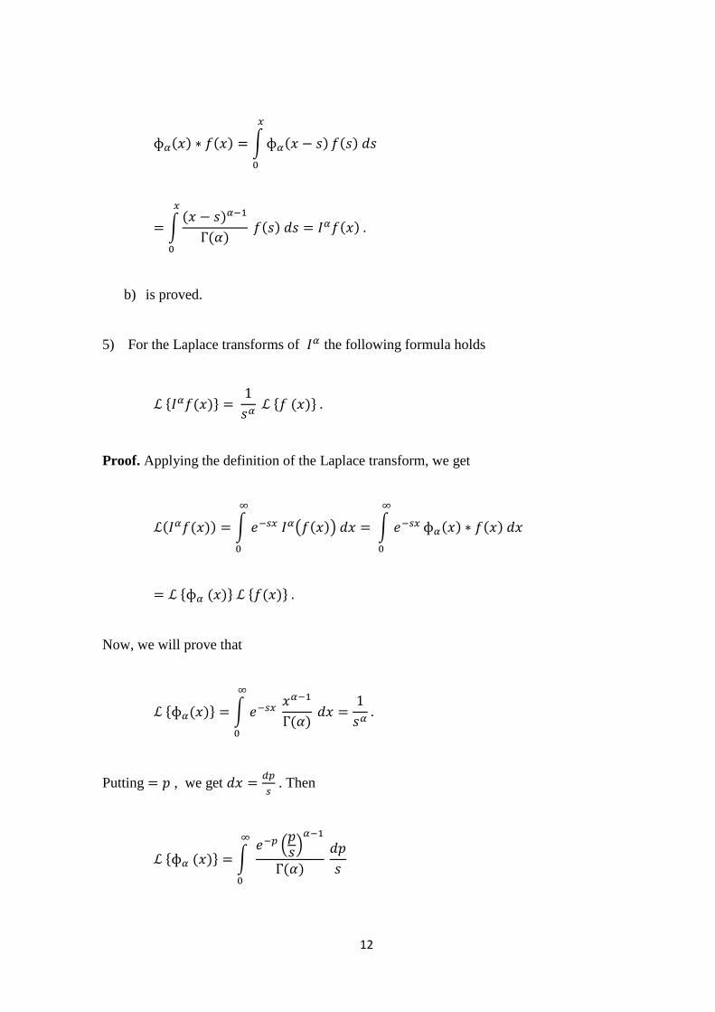
12
( ) ( ) ∫ ( )
( )
∫( )
( )
( ) ( )
b) is proved.
5) For the Laplace transforms of the following formula holds
* ( )+
* ( )+
Proof. Applying the definition of the Laplace transform, we get
( ( )) ∫ ( ( ))
∫
( ) ( )
* ( )+ * ( )+
Now, we will prove that
* ( )+ ∫
( )
Putting , we get
. Then
* ( )+ ∫ .
/
( )
13
( )
∫
( )
( )
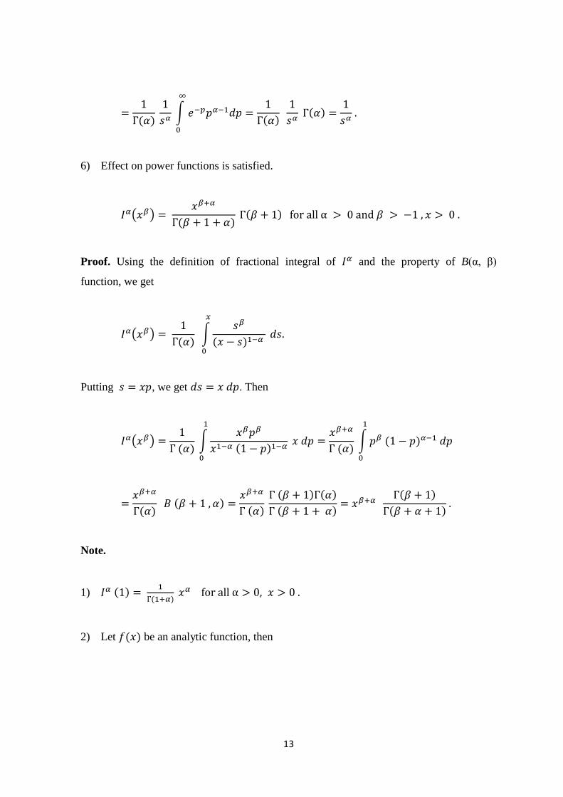
6) Effect on power functions is satisfied.
( )
( ) ( )
Proof. Using the definition of fractional integral of and the property of B(α, )
function, we get
( )
( ) ∫
( )
Putting , we get . Then
( )
( ) ∫
( )
( ) ∫ ( )
( ) ( )
( ) ( ) ( )
( )
( )
( )
Note.
1) ( )
( )
2) Let ( ) be an analytic function, then
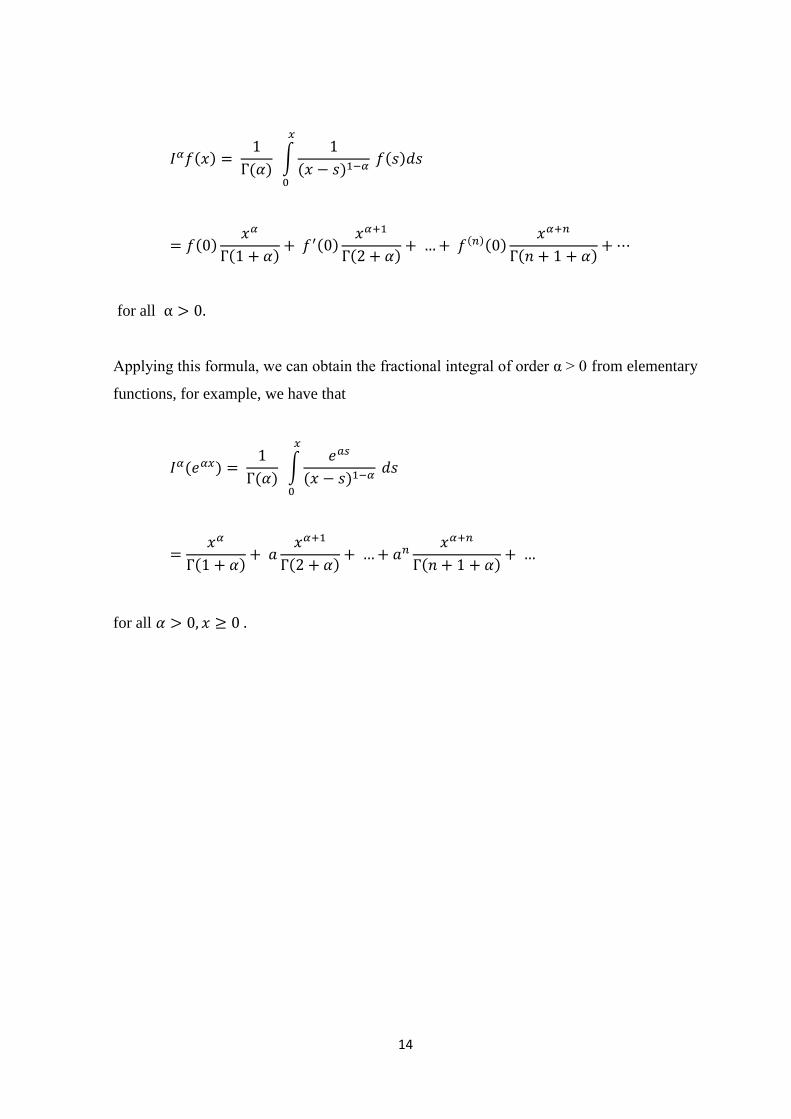
14
( )
( ) ∫
( ) ( )
( )
( ) ( )
( ) ( )( )
( )
for all
Applying this formula, we can obtain the fractional integral of order α > 0 from elementary
functions, for example, we have that
( )
( ) ∫
( )
( )
( )
( )
for all
15
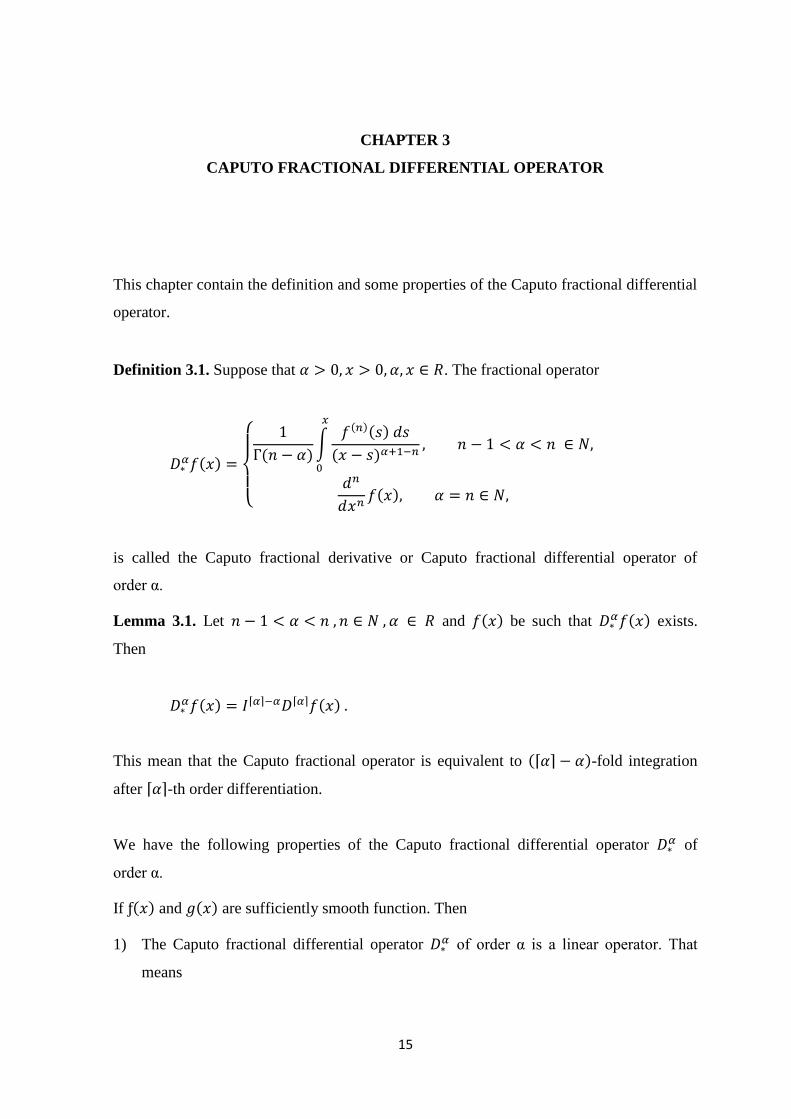
CHAPTER 3
CAPUTO FRACTIONAL DIFFERENTIAL OPERATOR
This chapter contain the definition and some properties of the Caputo fractional differential
operator.
Definition 3.1. Suppose that . The fractional operator
( )
{
( )∫
( )( )
( )
( )
is called the Caputo fractional derivative or Caputo fractional differential operator of
order α.
Lemma 3.1. Let and ( ) be such that ( ) exists.
Then
( ) ⌈ ⌉ ⌈ ⌉ ( )
This mean that the Caputo fractional operator is equivalent to (⌈ ⌉ )-fold integration
after ⌈ ⌉-th order differentiation.
We have the following properties of the Caputo fractional differential operator of
order α.
If ( ) and ( ) are sufficiently smooth function. Then
1) The Caputo fractional differential operator of order α is a linear operator. That
means
16
( ( ) ( ))
( ) ( )
Proof. Using the definition of , we get
( ( ) ( ))
Г(⌈ ⌉ )∫
( ) ⌈ ⌉
⌈ ⌉
⌈ ⌉, ( ) ( )-
(⌈ ⌉ )∫
( ) ⌈ ⌉
⌈ ⌉
⌈ ⌉ ( )
(⌈ ⌉ )∫
( ) ⌈ ⌉
⌈ ⌉
⌈ ⌉ ( )
( )
( )
2) The following non-semigroup properties hold
( )
( )
Proof. Let
( ) . Then applying the definition, we get
( ) (
( ))
( )
Г .
/ ∫
( )
( )
Г . /
∫
( )
√
√
17
(
( ))
4 √
√ 5
√
and
( )
Г . /
∫
( )
⌈ ⌉
⌈ ⌉( )
Г . /
∫
( )
( )
We see that
(
( ))
√
( )
3) The following non-commutative properties hold
Suppose that and ( ) exists. Then in general
( )
( ) ( )
Proof. Using the definition of , we get
( )
( ( ))
(⌈ ⌉ )∫
⌈ ⌉ ( )
( ) ⌈ ⌉
and
( )
((⌈ ⌉ ) ( )∫
⌈ ⌉ ( )
( ) (⌈ ⌉ ) ( )
18
(⌈ ⌉ )∫
( ) ⌈ ⌉
⌈ ⌉ ( )
Corollary 3.1. Suppose that ( ) ( )
and the function ( ) is such that ( ) exists. Then
( )
( )
Proof. Substitute for and for in
( )
( ) ( )
Then
( ) ( )
( ) ( ) ( )
( ) ( )
This means
( )
( ) ( )
4) For any constant properties hold
( )
Proof. Using the definition of , we get
( )
(⌈ ⌉ )∫
( ) ⌈ ⌉
⌈ ⌉
⌈ ⌉( )
5) For the Laplace transform of the following formula holds
19
* ( )+ * ( )+ ∑ ( )( )
Proof. Applying the definition of Laplace transform, we get
* ( )+ ∫ (
( ))
∫
(⌈ ⌉ )∫
( ) ⌈ ⌉ ⌈ ⌉( )
Changing the order of integration and using
* + * +, we get
* ( )+
(⌈ ⌉ )∫ ⌈ ⌉( )
∫
( ) ⌈ ⌉
Putting , we get
(⌈ ⌉ )∫
⌈ ⌉( ) ∫
⌈ ⌉
Now, we will obtain the integral
( ) ∫
⌈ ⌉
Putting , we get
and
21
( ) ⌈ ⌉ ∫ ⌈ ⌉
⌈ ⌉ (⌈ ⌉ )
Therefore
(
(⌈ ⌉ )∫
⌈ ⌉( ) ) . ⌈ ⌉ (⌈ ⌉ )/
* ( )+
{ * ( )+ ∑
( )}
* ( )+ ∑
( )
6) The Riemann-Liouville integral operator and the Caputo fractional differential
operator are inverse operators in the sense that
a) ( ) ( )
Proof. Using the definition of , we get
( ) ⌈ ⌉ ⌈ ⌉ ⌈ ⌉ ⌈ ⌉ ( ) ⌈ ⌉ ( ⌈ ⌉ ⌈ ⌉) ⌈ ⌉ ( )
⌈ ⌉ ⌈ ⌉ ( )
From that it follows
21
( )
(⌈ ⌉ )∫
⌈ ⌉ ( )
( ) ⌈ ⌉
(⌈ ⌉ )∫
( ) ⌈ ⌉
(
( ⌈ ⌉)∫
( )
( ) ⌈ ⌉
)
(⌈ ⌉ )∫
( ) ⌈ ⌉ (
( ⌈ ⌉ )∫
( )
( )⌈ ⌉
)
Now, we obtain the formula for
(
( ⌈ ⌉ )∫
( )
( )⌈ ⌉
)
We have that
( ⌈ ⌉)∫
( )
( )⌈ ⌉
( ⌈ ⌉)∫ ( )
( ) ⌈ ⌉
⌈ ⌉
( ⌈ ⌉) ( ⌈ ⌉)
* ( ) ⌈ ⌉ ∫ ( )( ) ⌈ ⌉
+
22
( ⌈ ⌉)* ( ) ⌈ ⌉ ∫ ( )( ) ⌈ ⌉
+
Therefore,
(
( ⌈ ⌉)∫
( )
( )⌈ ⌉
)
( ⌈ ⌉)
* ( )( ⌈ ⌉) ⌈ ⌉ ∫ ( )( ⌈ ⌉)( ) ⌈ ⌉
+
( ⌈ ⌉)* ( ) ⌈ ⌉ ∫ ( )( ) ⌈ ⌉
+
Applying this formula, we get
( )
(⌈ ⌉ )∫
( ) ⌈ ⌉
,
( ⌈ ⌉)* ( ) ⌈ ⌉ ∫ ( )( ) ⌈ ⌉
+-
(⌈ ⌉ ) ( ⌈ ⌉) { ( ) ∫
⌈ ⌉
( ) ⌈ ⌉
}
23
(⌈ ⌉ ) ( ⌈ ⌉)
{
∫
( ) ⌈ ⌉
∫ ( )( ) ⌈ ⌉
}
Now, we will obtain the integral
( ) ∫ ( ) ⌈ ⌉
( ) ⌈ ⌉
Putting , we get
( ) ∫( ) ⌈ ⌉
( ) ⌈ ⌉
( ) ( ⌈ ⌉ ⌈ ⌉ )
( ) ( ⌈ ⌉ ) (⌈ ⌉ ) ( )
Now, we will obtain the integral
(( )( )) ∫ ∫ ( )
( ) ⌈ ⌉ ( )⌈ ⌉
Changing the order of integral and using
, - , -, we get
(( )( )) ∫ ( )
∫
( ) ⌈ ⌉ ( )⌈ ⌉
Putting , we get and
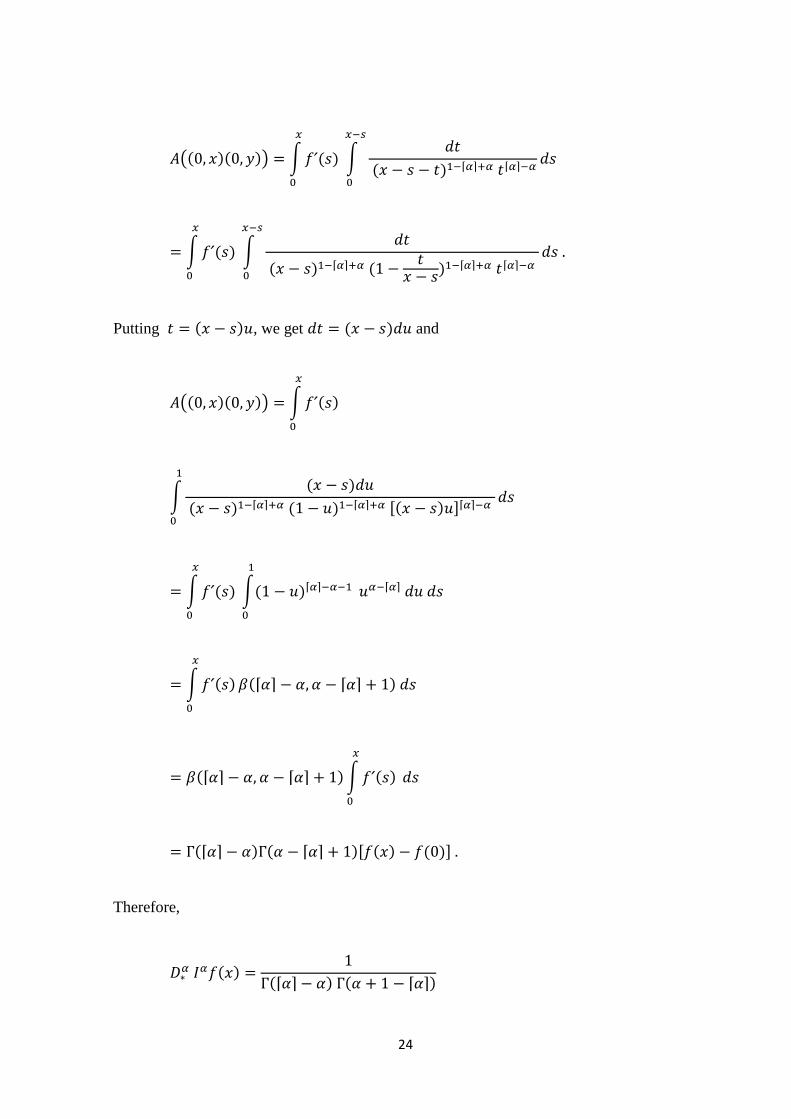
24
(( )( )) ∫ ( )
∫
( ) ⌈ ⌉ ⌈ ⌉
∫ ( )
∫
( ) ⌈ ⌉ (
) ⌈ ⌉ ⌈ ⌉
Putting ( ) , we get ( ) and
(( )( )) ∫ ( )
∫( )
( ) ⌈ ⌉ ( ) ⌈ ⌉ ,( ) -⌈ ⌉
∫ ( )
∫( )⌈ ⌉
⌈ ⌉
∫ ( )
(⌈ ⌉ ⌈ ⌉ )
(⌈ ⌉ ⌈ ⌉ ) ∫ ( )
(⌈ ⌉ ) ( ⌈ ⌉ ), ( ) ( )-
Therefore,
( )
(⌈ ⌉ ) ( ⌈ ⌉)
25
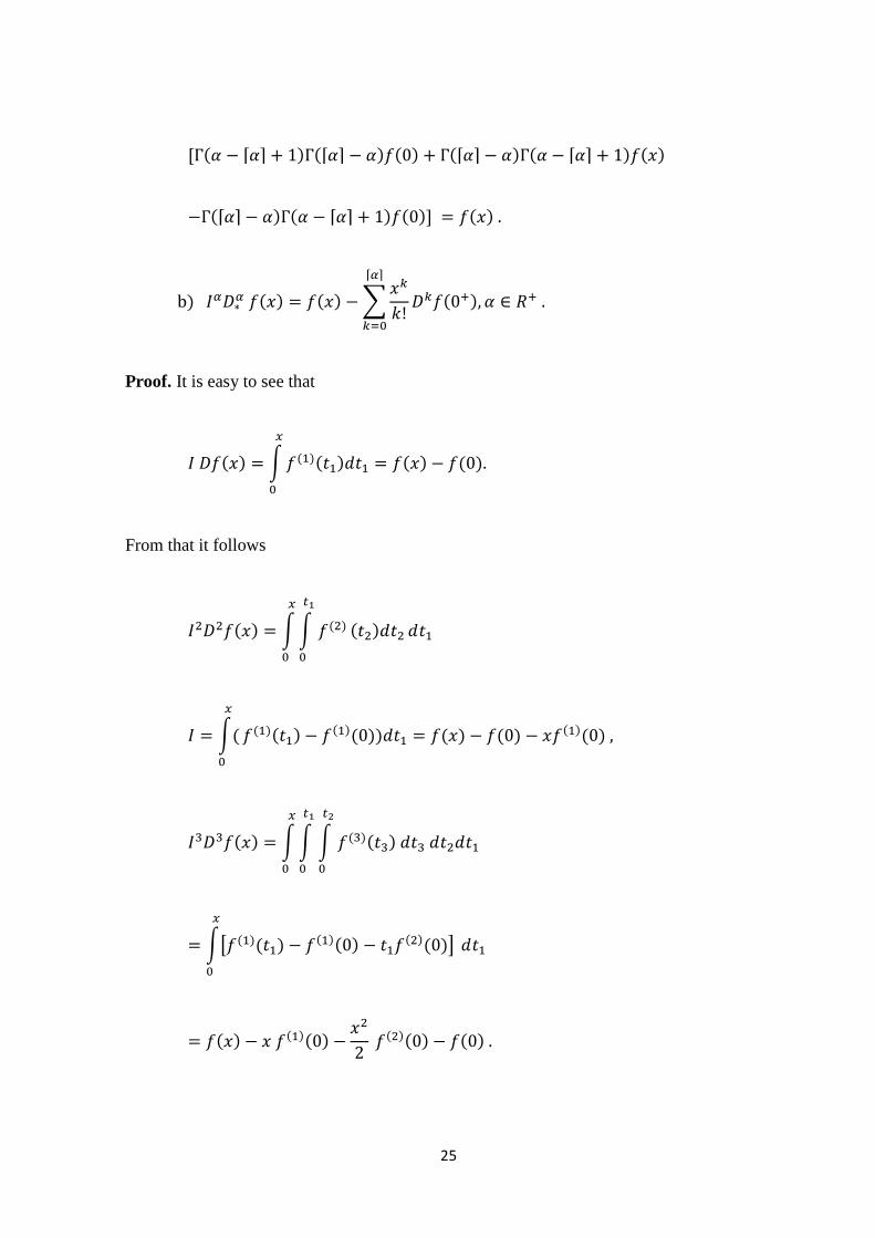
, ( ⌈ ⌉ ) (⌈ ⌉ ) ( ) (⌈ ⌉ ) ( ⌈ ⌉ ) ( )
(⌈ ⌉ ) ( ⌈ ⌉ ) ( )- ( )
) ( ) ( ) ∑
⌈ ⌉
( )
Proof. It is easy to see that
( ) ∫ ( )( ) ( ) ( )
From that it follows
( ) ∫ ∫ ( )
( )
∫(
( )( ) ( )( )) ( ) ( ) ( )( )
( ) ∫ ∫ ∫ ( )( )
∫[ ( )( ) ( )( ) ( )( )]
( ) ( )( )
( )( ) ( )
26
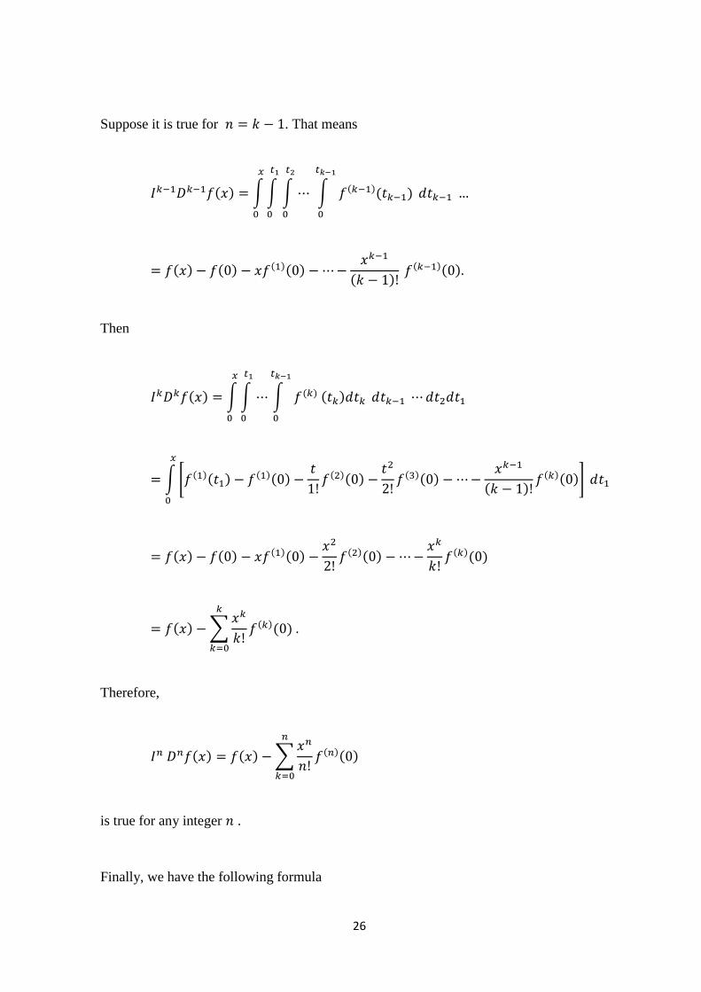
Suppose it is true for . That means
( ) ∫ ∫ ∫
∫ ( )( )
( ) ( ) ( )( )
( ) ( )( )
Then
( ) ∫ ∫ ∫ ( ) ( )
∫ 6 ( )( ) ( )( )
( )( )
( )( )
( ) ( )( )7
( ) ( ) ( )( )
( )( )
( )( )
( ) ∑
( )( )
Therefore,
( ) ( ) ∑
( )( )
is true for any integer .
Finally, we have the following formula
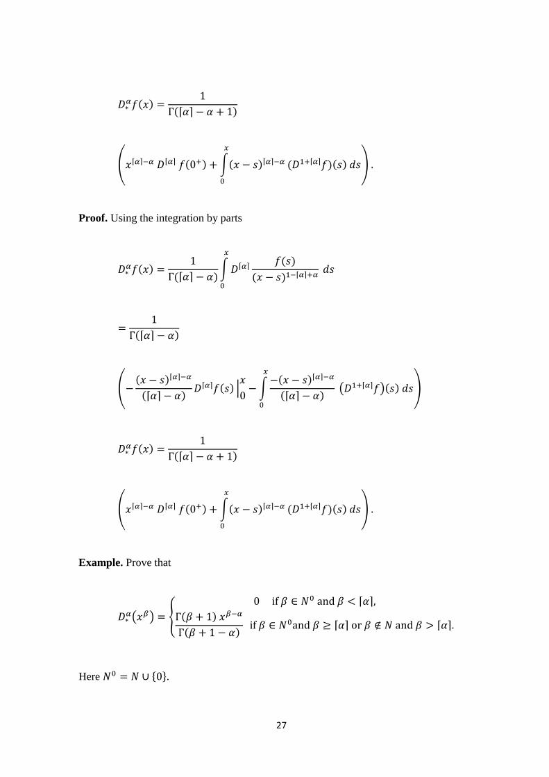
27
( )
(⌈ ⌉ )
( ⌈ ⌉ ⌈ ⌉ ( ) ∫( )⌈ ⌉
( ⌈ ⌉ )( ) )
Proof. Using the integration by parts
( )
(⌈ ⌉ )∫ ⌈ ⌉
( )
( ) ⌈ ⌉
(⌈ ⌉ )
( ( )⌈ ⌉
(⌈ ⌉ ) ⌈ ⌉ ( ) |
∫
( )⌈ ⌉
(⌈ ⌉ )
( ⌈ ⌉ )( ) )
( )
(⌈ ⌉ )
( ⌈ ⌉ ⌈ ⌉ ( ) ∫( )⌈ ⌉
( ⌈ ⌉ )( ) )
Example. Prove that
( ) ,
⌈ ⌉
( )
( ) ⌈ ⌉ ⌈ ⌉
Here * +.
28
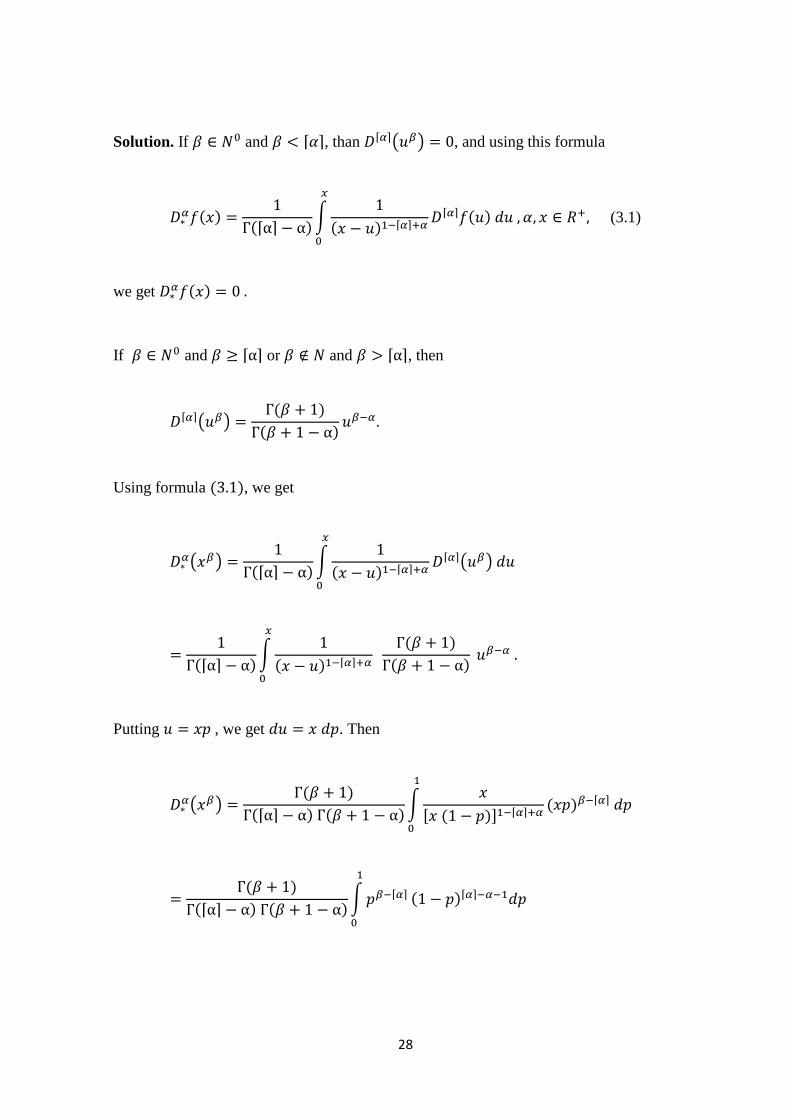
Solution. If and ⌈ ⌉, than ⌈ ⌉( ) , and using this formula
( )
(⌈ ⌉ )∫
( ) ⌈ ⌉
⌈ ⌉ ( ) (3.1)
we get ( )
If and ⌈ ⌉ or and ⌈ ⌉, then
⌈ ⌉( ) ( )
( )
Using formula ( ), we get
( )
(⌈ ⌉ )∫
( ) ⌈ ⌉ ⌈ ⌉( )
(⌈ ⌉ )∫
( ) ⌈ ⌉
( )
( )
Putting , we get . Then
( )
( )
(⌈ ⌉ ) ( )∫
, ( )- ⌈ ⌉ ( ) ⌈ ⌉
( )
(⌈ ⌉ ) ( )∫ ⌈ ⌉
( )⌈ ⌉
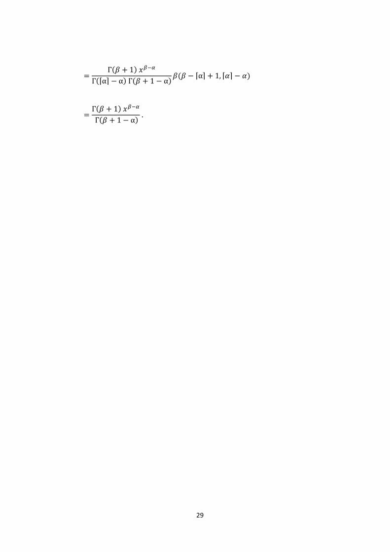
29
( )
(⌈ ⌉ ) ( ) ( ⌈ ⌉ ⌈ ⌉ )
( )
( )
31
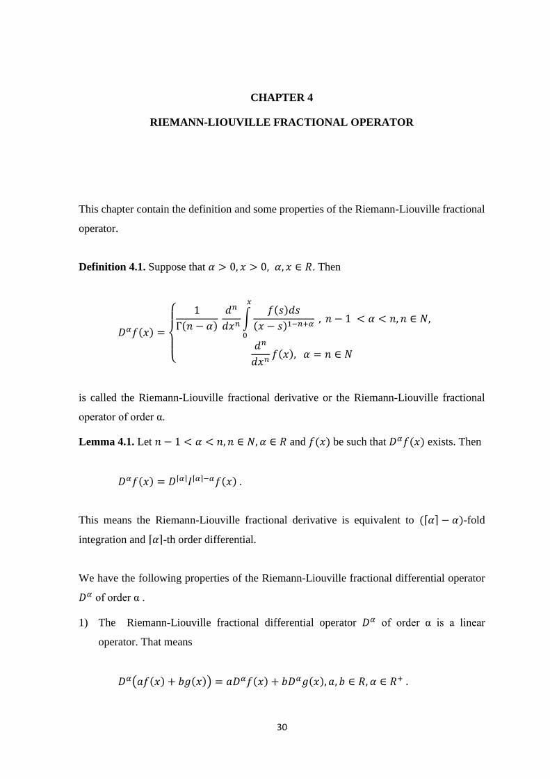
CHAPTER 4
RIEMANN-LIOUVILLE FRACTIONAL OPERATOR
This chapter contain the definition and some properties of the Riemann-Liouville fractional
operator.
Definition 4.1. Suppose that . Then
( )
{
( )
∫
( )
( )
( )
is called the Riemann-Liouville fractional derivative or the Riemann-Liouville fractional
operator of order α.
Lemma 4.1. Let and ( ) be such that ( ) exists. Then
( ) ⌈ ⌉ ⌈ ⌉ ( )
This means the Riemann-Liouville fractional derivative is equivalent to (⌈ ⌉ )-fold
integration and ⌈ ⌉-th order differential.
We have the following properties of the Riemann-Liouville fractional differential operator
of order α .
1) The Riemann-Liouville fractional differential operator of order α is a linear
operator. That means
( ( ) ( )) ( ) ( )
31
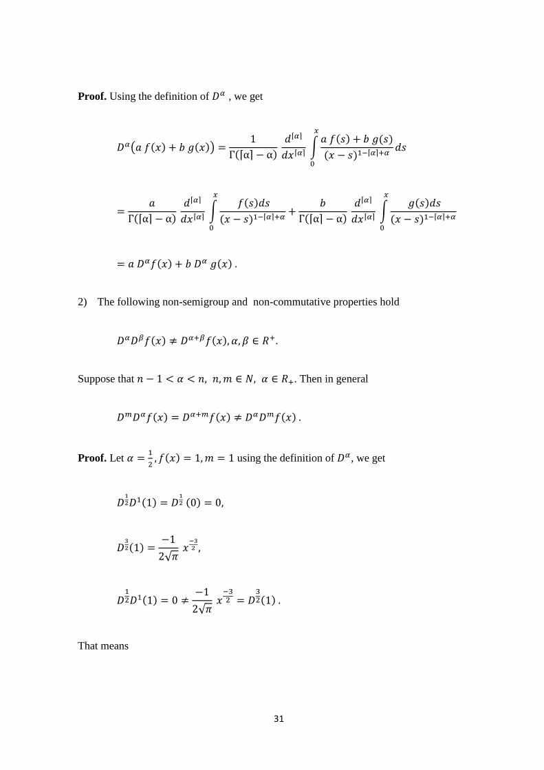
Proof. Using the definition of , we get
( ( ) ( ))
(⌈ ⌉ )
⌈ ⌉
⌈ ⌉ ∫
( ) ( )
( ) ⌈ ⌉
(⌈ ⌉ )
⌈ ⌉
⌈ ⌉ ∫
( )
( ) ⌈ ⌉
(⌈ ⌉ )
⌈ ⌉
⌈ ⌉ ∫
( )
( ) ⌈ ⌉
( ) ( )
2) The following non-semigroup and non-commutative properties hold
( ) ( )
Suppose that . Then in general
( ) ( ) ( )
Proof. Let
( ) using the definition of , we get
( )
( )
( )
√
( )
√
( )
That means
32
( )
( ) (non-semigroup)
and
( ) (
√
)
√
( )
√
( )
That means
( )
( ) (non-commutative) .
3) For any constant C, the formulas hold
( )
( )
Proof. Using the definition of , we get
( )
(⌈ ⌉ )
⌈ ⌉
⌈ ⌉∫
( ) ⌈ ⌉
( )
6
( )
( ) |
7
( )
( )
( )
4) For the Laplace transform of the following formula holds
33
* ( )+ * ( )+ ∑
, ( )-
Proof. Applying the definition of Laplace transform, we get
* ( )+ ∫
, ( )-
∫
{
( )
∫
( )
( )
}
( )∫
{
∫
( )
( )
}
( ) {∫
( )
( )
}
( ){ ∫
( )
( )
}
( ){
∫
( )
( )
}
( )∫
∫ ( )
( )
( )
( ( ))
we obtain formula for the integral
34
( )
( )∫
∫ ( )
( )
Changing the order of integration and using
, - , -, we get
( )
( )∫ ( )
∫
( )
Putting , we get
( )
( )∫ ( )
∫
Now, we will obtain the integral
( ) ∫
Putting , we get
( ) ∫
. /
∫
( )
Therefore,
35
( )
( )∫ ( )
( ( )) ∫ ( )
* ( )+
and
* ( )+ * ( )+ ∑
, ( )-
5) In general the two operators Riemann - Liouville and Caputo, do not coincide.
Actually,
( ) ⌈ ⌉ ⌈ ⌉ ( ) ⌈ ⌉ ⌈ ⌉ ( ) ( )
But, we have the following formula
( ) ( ( ) ∑
( )( ))
Proof. The well-known Taylor series expansion about the point 0 is
( ) ( ) ( )( )
( )( )
( )( )
( ) ( )( )
∑
( )
( )( )
36
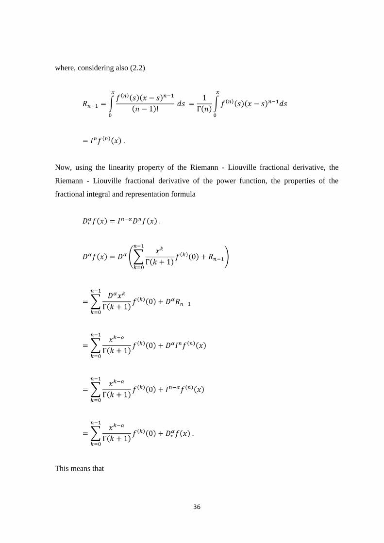
where, considering also (2.2)
∫ ( )( )( )
( )
( )∫ ( )( )( )
( )( )
Now, using the linearity property of the Riemann - Liouville fractional derivative, the
Riemann - Liouville fractional derivative of the power function, the properties of the
fractional integral and representation formula
( ) ( )
( ) (∑
( )
( )( ) )
∑
( )
( )( )
∑
( )
( )( ) ( )( )
∑
( )
( )( ) ( )( )
∑
( )
( )( ) ( )
This means that
37
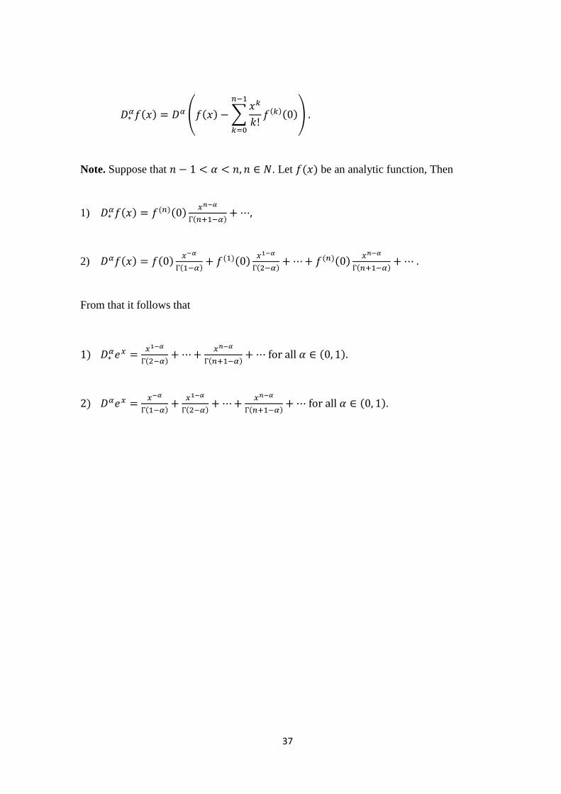
( ) ( ( ) ∑
( )( ))
Note. Suppose that . Let ( ) be an analytic function, Then
1) ( ) ( )( )
( )
2) ( ) ( )
( ) ( )( )
( ) ( )( )
( )
From that it follows that
1)
( )
( ) for all ( )
2)
( )
( )
( ) for all ( )
38
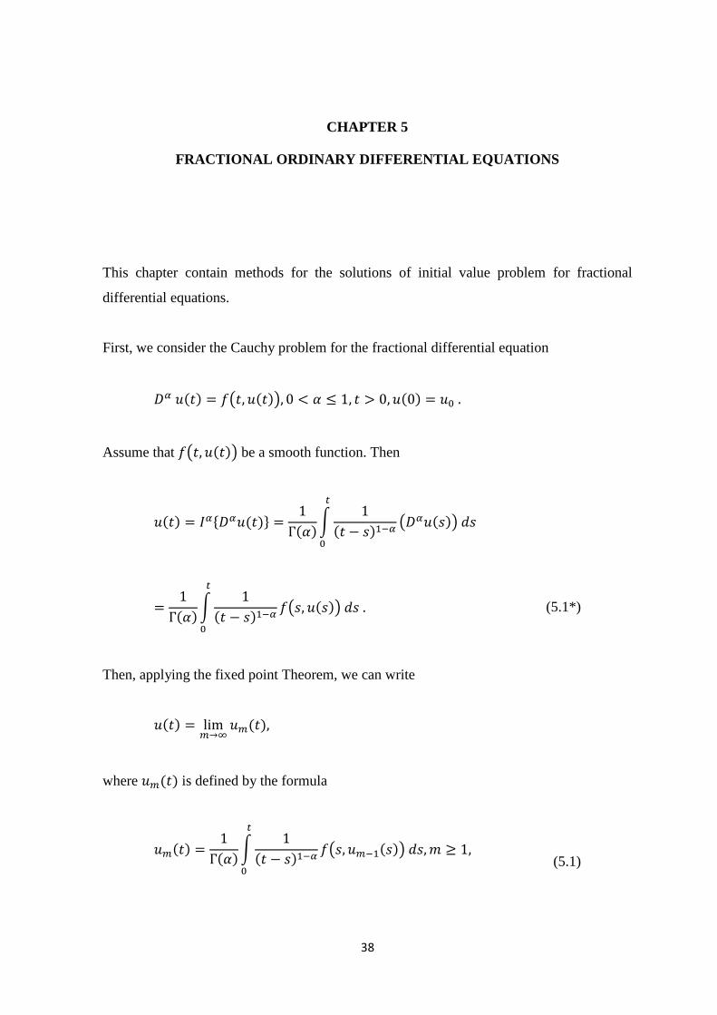
CHAPTER 5
FRACTIONAL ORDINARY DIFFERENTIAL EQUATIONS
This chapter contain methods for the solutions of initial value problem for fractional
differential equations.
First, we consider the Cauchy problem for the fractional differential equation
( ) ( ( )) ( )
Assume that ( ( )) be a smooth function. Then
( ) * ( )+
( )∫
( )
( ( ))
( )∫
( )
( ( )) (5.1*)
Then, applying the fixed point Theorem, we can write
( )
( )
where ( ) is defined by the formula
( )
( )∫
( )
( ( ))
(5.1)
39
( )
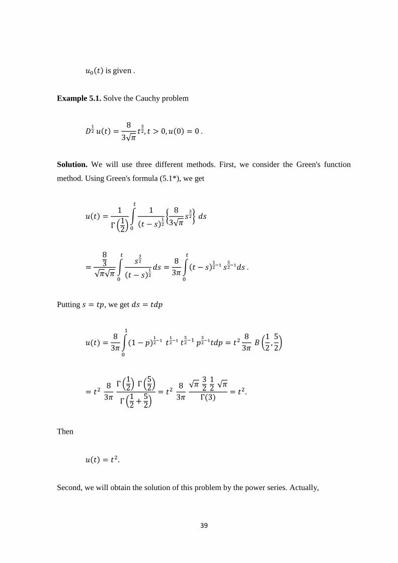
Example 5.1. Solve the Cauchy problem
( )
√
( )
Solution. We will use three different methods. First, we consider the Green's function
method. Using Green's formula (5.1*), we get
( )
. /
∫
( )
{
√
}
√ √ ∫
( )
∫( )
Putting , we get
( )
∫( )
(
)
.
/ .
/
.
/
√
√
( )
Then
( )
Second, we will obtain the solution of this problem by the power series. Actually,
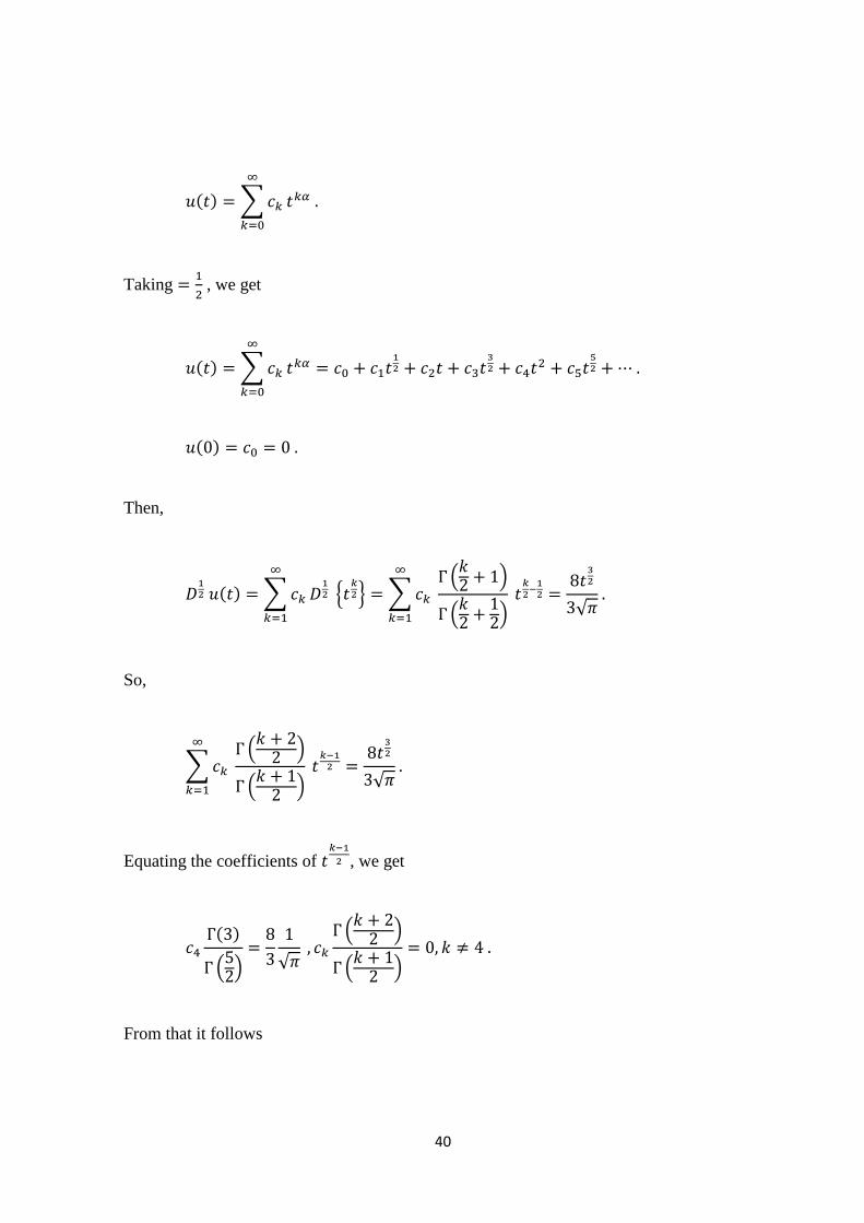
41
( ) ∑
Taking
, we get
( ) ∑
( )
Then,
( ) ∑
2
3 ∑
.
/
.
/
√
So,
∑
.
/
.
/
√
Equating the coefficients of
, we get
( )
. /
√
.
/
.
/
From that it follows
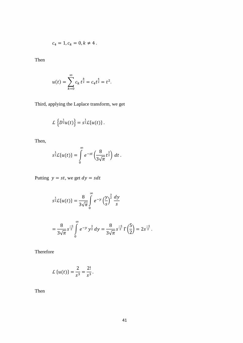
41
Then
( ) ∑
Third, applying the Laplace transform, we get
2 ( )3
* ( )+
Then,
* ( )+ ∫
(
√
)
Putting , we get
* ( )+
√ ∫
.
/
√
∫
√
(
)
Therefore
* ( )+
Then
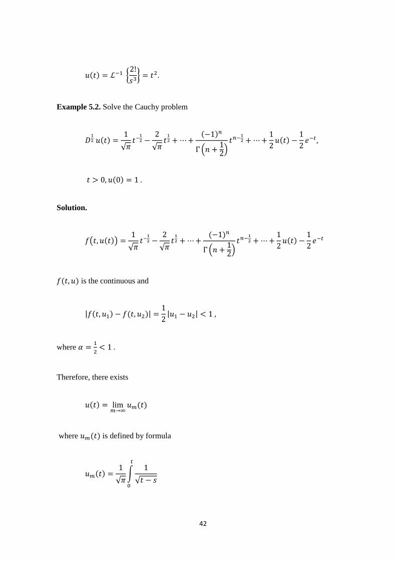
42
( ) {
}
Example 5.2. Solve the Cauchy problem
( )
√
√
( )
. /
( )
( )
Solution.
( ( ))
√
√
( )
. /
( )
( ) is the continuous and
| ( ) ( )|
| |
where
Therefore, there exists
( )
( )
where ( ) is defined by formula
( )
√ ∫
√
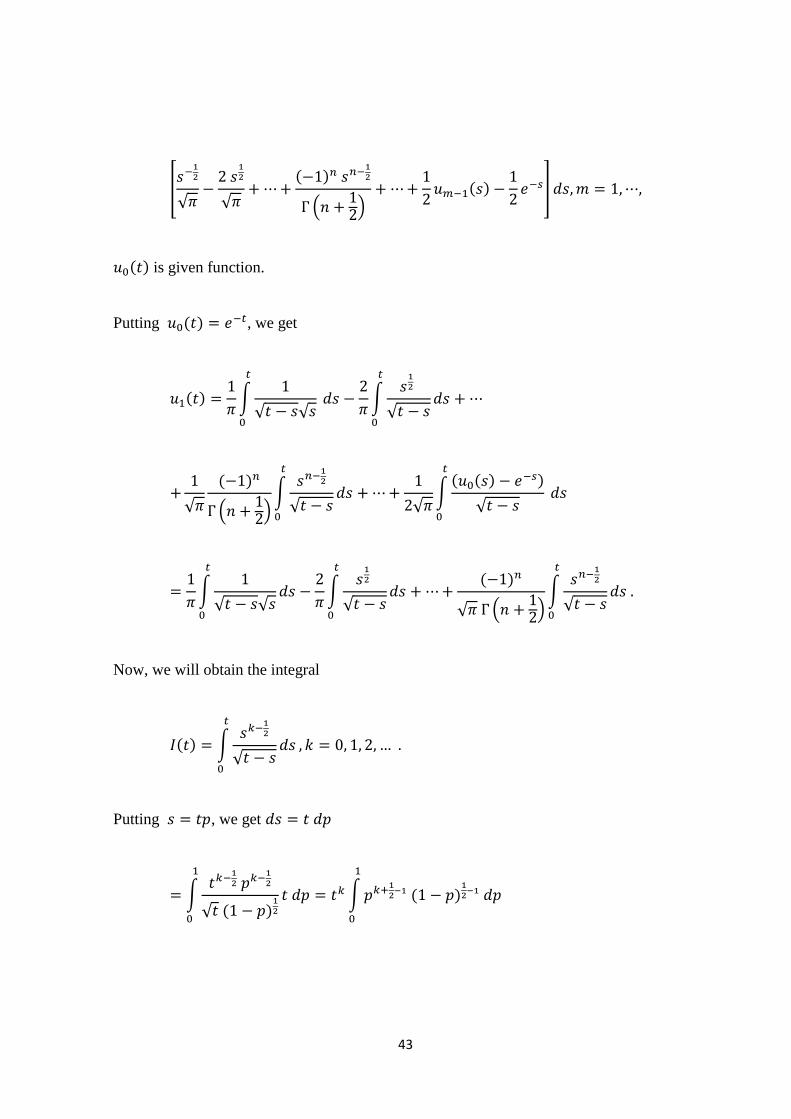
43
*
√
√
( )
. /
( )
+
( ) is given function.
Putting ( ) , we get
( )
∫
√ √
∫
√
√
( )
. /
∫
√
√ ∫
( ( ) )
√
∫
√ √
∫
√
( )
√ . /
∫
√
Now, we will obtain the integral
( ) ∫
√
Putting , we get
∫
√ ( )
∫
( )
44
(
)
. / .
/
( )
Using this formula, we get
( ) .
/
. /
( )
√ . /
.
/ .
/
. /
( )
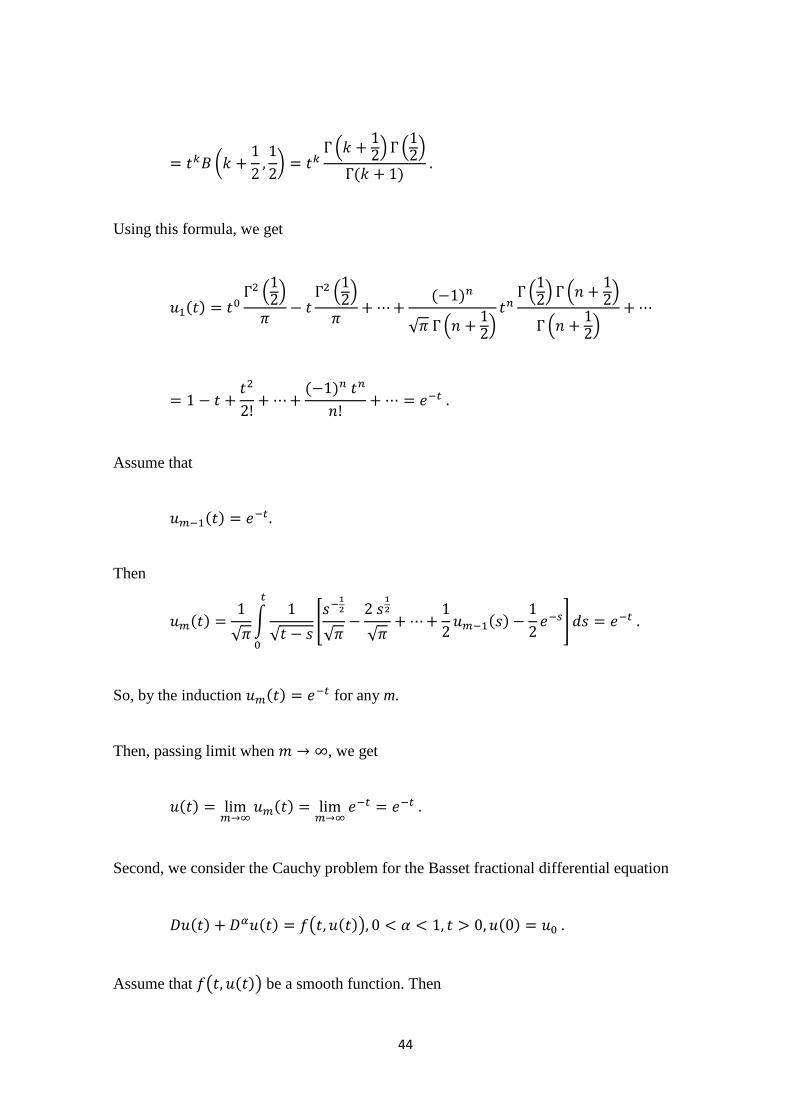
Assume that
( )
Then
( )
√ ∫
√
[
√
√
( )
]
So, by the induction ( ) for any m.
Then, passing limit when , we get
( )
( )
Second, we consider the Cauchy problem for the Basset fractional differential equation
( ) ( ) ( ( )) ( )
Assume that ( ( )) be a smooth function. Then
45
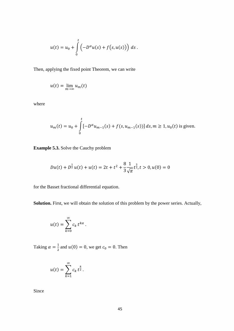
( ) ∫ . ( ) ( ( ))/
Then, applying the fixed point Theorem, we can write
( )
( )
where
( ) ∫, ( ) ( ( ))-
( )
Example 5.3. Solve the Cauchy problem
( ) ( ) ( )
√
( )
for the Basset fractional differential equation.
Solution. First, we will obtain the solution of this problem by the power series. Actually,
( ) ∑
Taking
and ( ) , we get . Then
( ) ∑
Since
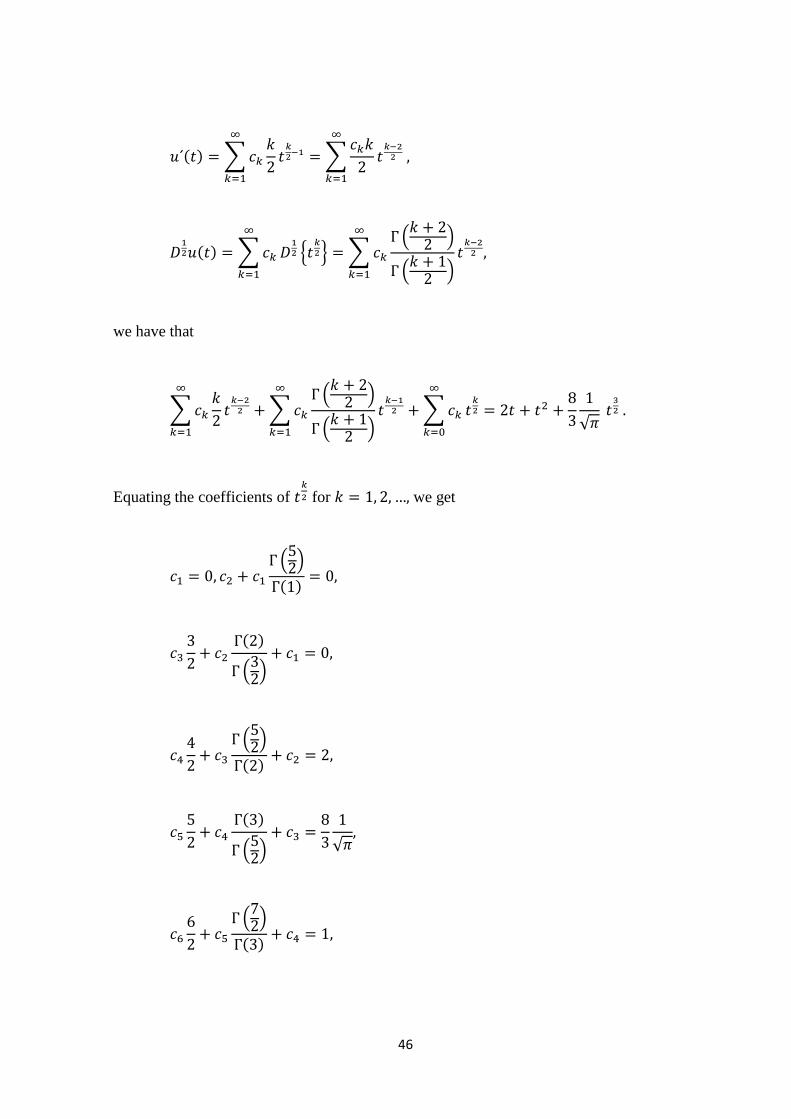
46
( ) ∑
∑
( ) ∑
2
3 ∑
.
/
.
/
we have that
∑
∑
.
/
.
/
∑
√
Equating the coefficients of
for we get
. /
( )
( )
. /
. /
( )
( )
. /
√
. /
( )
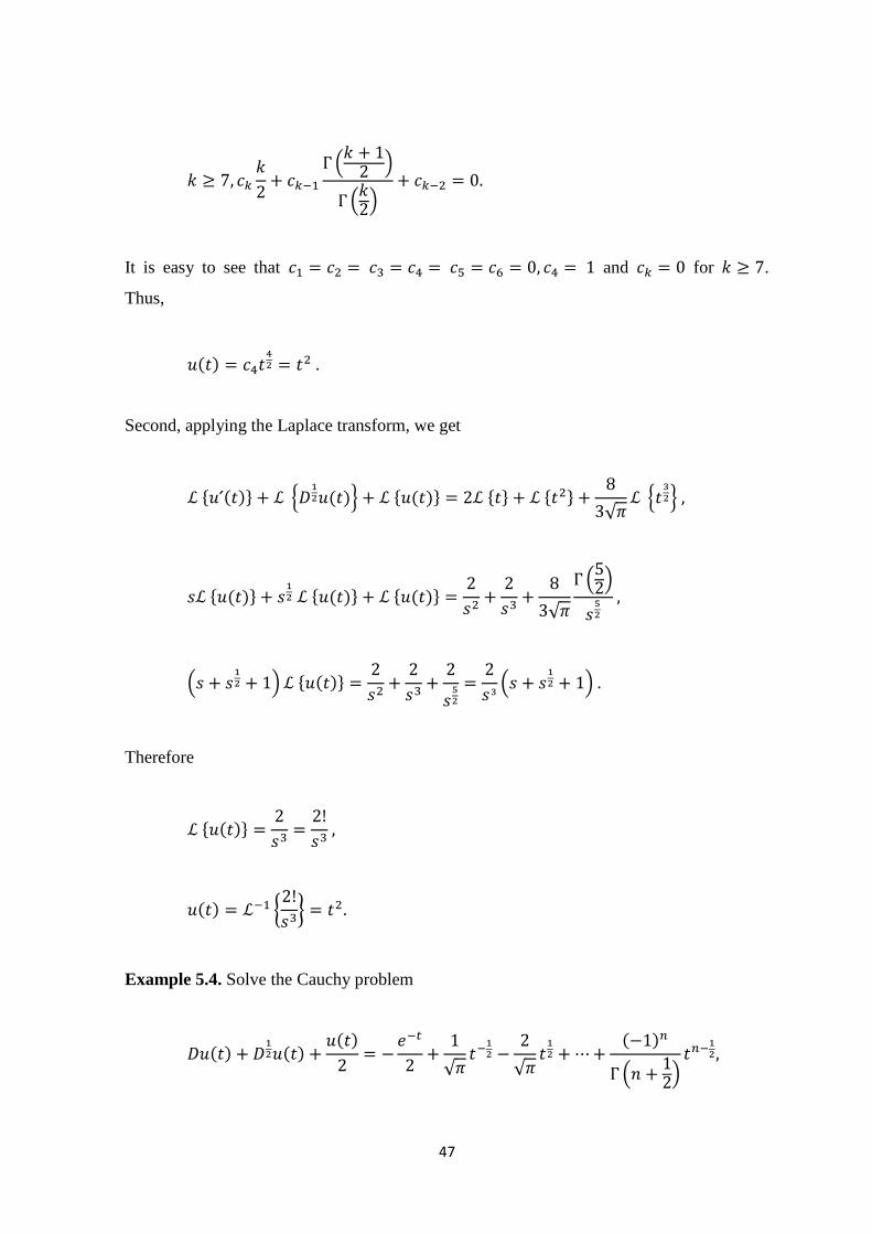
47
.
/
. /
It is easy to see that and for .
Thus,
( )
Second, applying the Laplace transform, we get
* ( )+ 2 ( )3 * ( )+ * + * +
√ 2
3
* ( )+ * ( )+ * ( )+
√
. /
. / * ( )+
.
/
Therefore
* ( )+
( ) {
}
Example 5.4. Solve the Cauchy problem
( ) ( )
( )
√
√
( )
. /
48
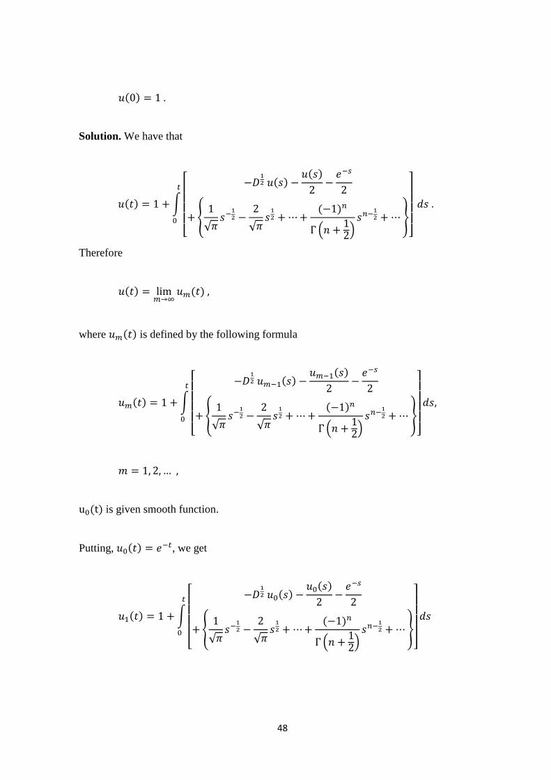
( )
Solution. We have that
( ) ∫
[
( )
( )
,
√
√
( )
. /
-
]
Therefore
( )
( )
where ( ) is defined by the following formula
( ) ∫
[
( )
( )
,
√
√
( )
.
/
-
]
( ) is given smooth function.
Putting, ( ) , we get
( ) ∫
[
( )
( )
,
√
√
( )
. /
-
]
49
∫
[
,
√
√
( )
. /
-
,
√
√
( )
. /
-
]
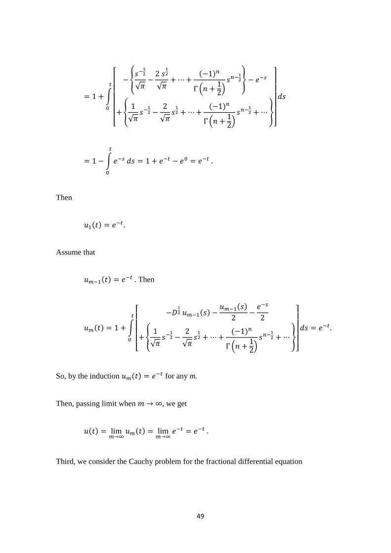
∫
Then
( )
Assume that
( ) Then
( ) ∫
[
( )
( )
,
√
√
( )
. /
-
]
So, by the induction ( ) for any m.
Then, passing limit when , we get
( )
( )
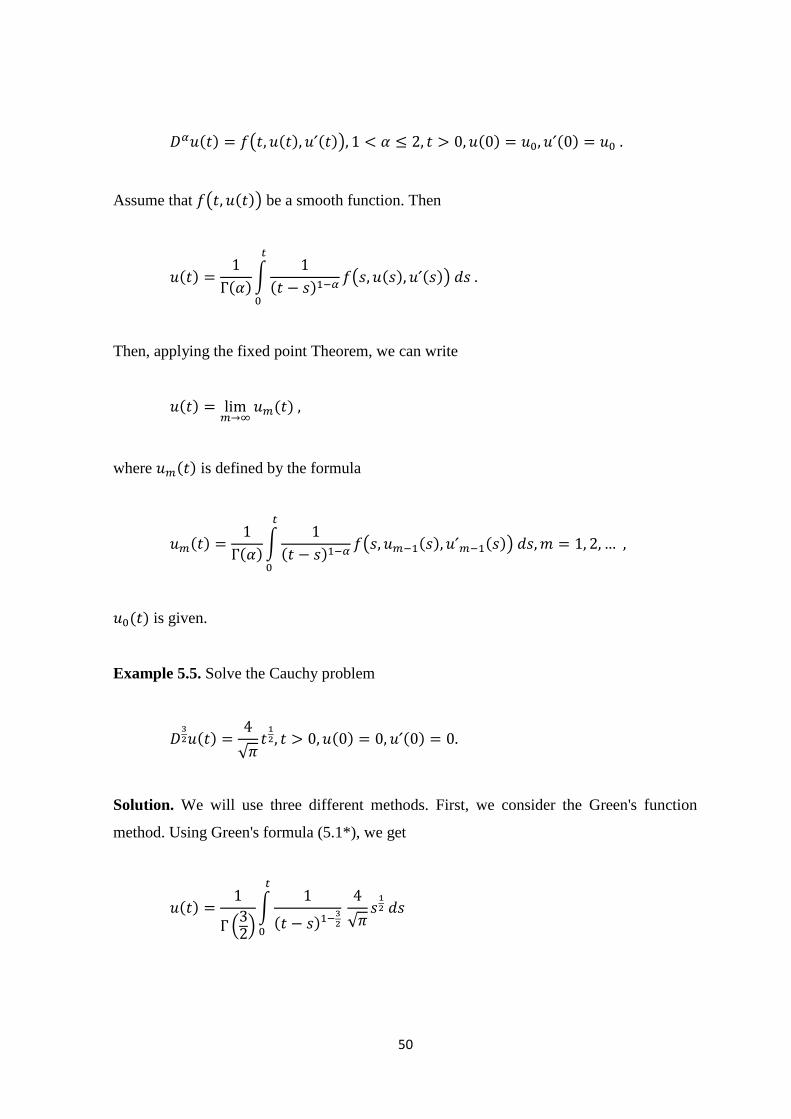
Third, we consider the Cauchy problem for the fractional differential equation
51
( ) ( ( ) ( )) ( ) ( )
Assume that ( ( )) be a smooth function. Then
( )
( )∫
( )
( ( ) ( ))
Then, applying the fixed point Theorem, we can write
( )
( )
where ( ) is defined by the formula
( )
( )∫
( )
( ( ) ( ))
( ) is given.
Example 5.5. Solve the Cauchy problem
( )
√
( ) ( )
Solution. We will use three different methods. First, we consider the Green's function
method. Using Green's formula (5.1*), we get
( )
. /
∫
( )
√
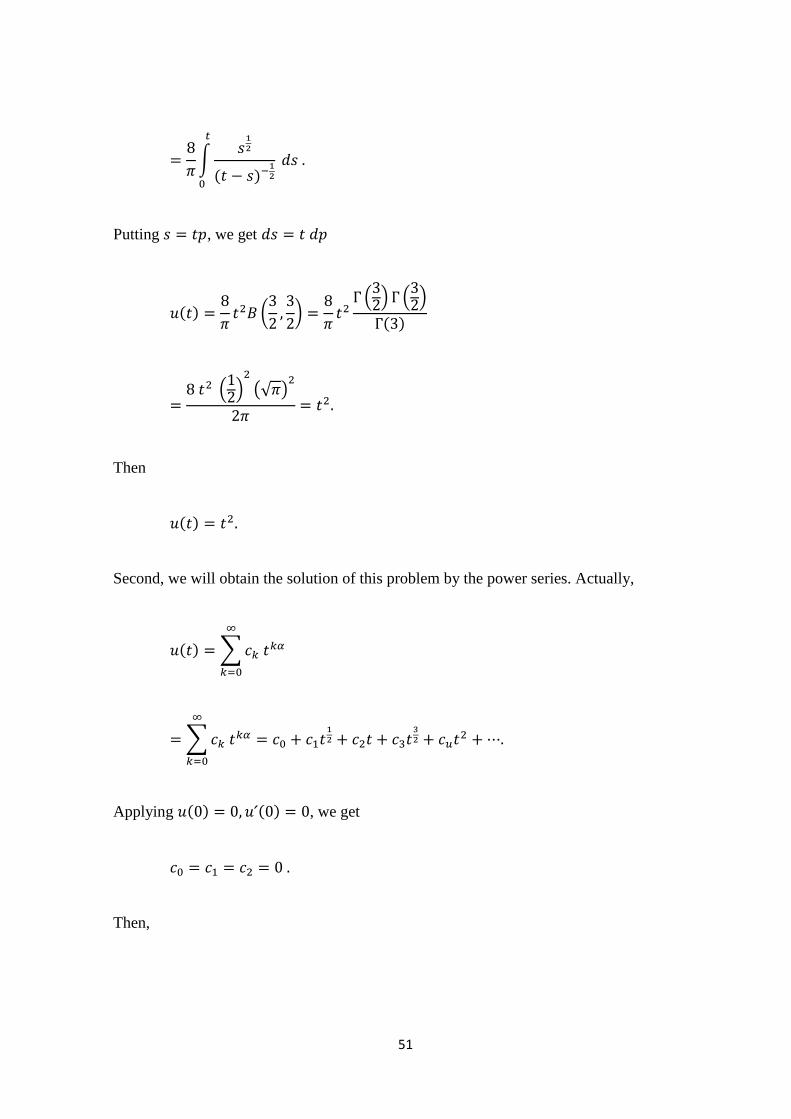
51
∫
( )
Putting , we get
( )
(
)
. / .
/
( )
.
/
(√ )
Then
( )
Second, we will obtain the solution of this problem by the power series. Actually,
( ) ∑
∑
Applying ( ) ( ) , we get
Then,
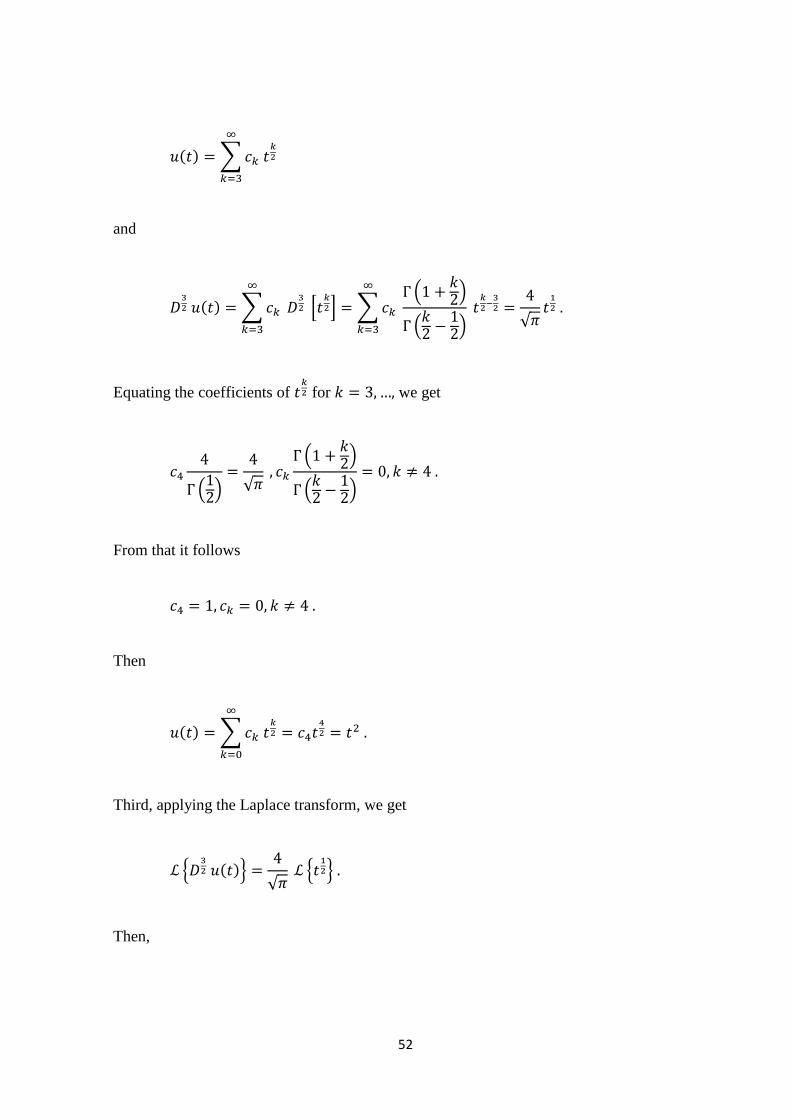
52
( ) ∑
and
( ) ∑
0
1 ∑
.
/
.
/
√
Equating the coefficients of for we get
. /
√
. /
.
/
From that it follows
Then
( ) ∑
Third, applying the Laplace transform, we get
2 ( )3
√ 2
3
Then,
53
* ( )+
√ .
/
√
√
Therefore
* ( )+
and
( ) {
}
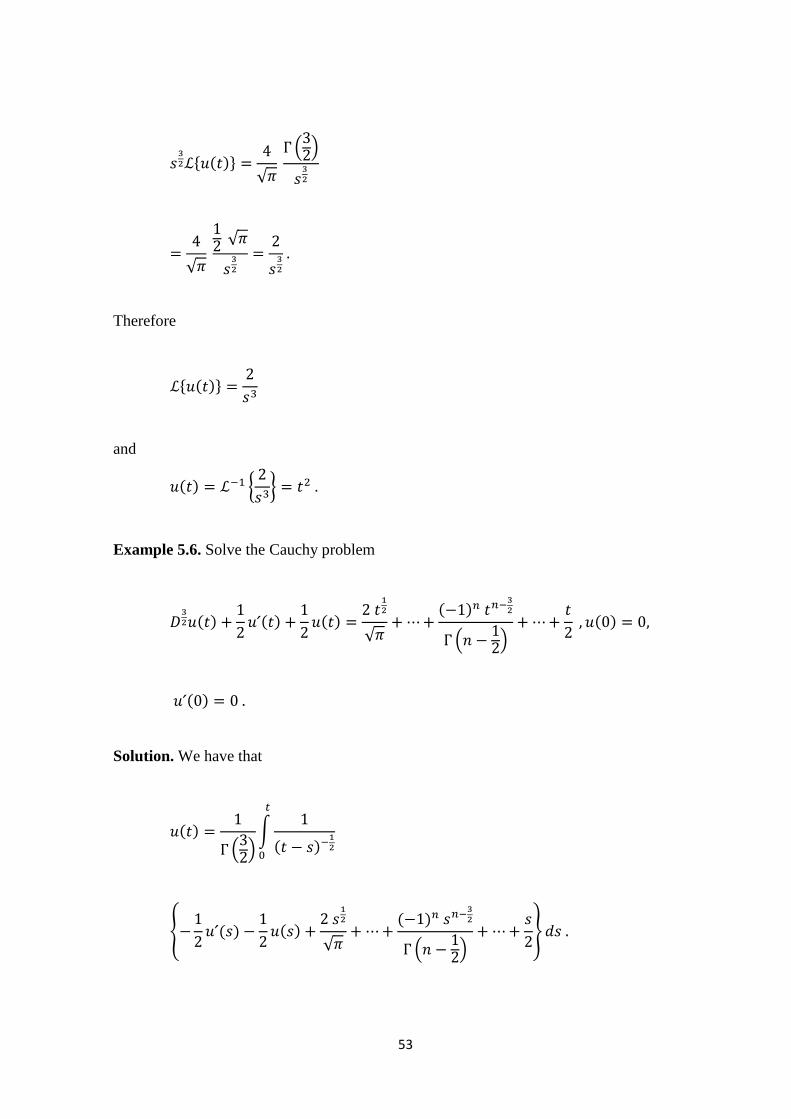
Example 5.6. Solve the Cauchy problem
( )
( )
( )
√
( )
. /
( )
( )
Solution. We have that
( )
. /
∫
( )
,
( )
( )
√
( )
. /
-
54
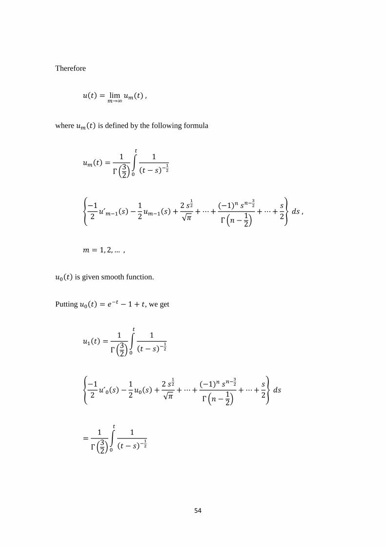
Therefore
( )
( )
where ( ) is defined by the following formula
( )
. /
∫
( )
,
( )
( )
√
( )
. /
-
( ) is given smooth function.
Putting ( ) , we get
( )
. /
∫
( )
,
( )
( )
√
( )
. /
-
. /
∫
( )
55
,
( )
( )
√
( )
. /
-
. /
∫
( )
,
√
( )
. /
-
∫
( )
( )
. / .
/
∫
( )
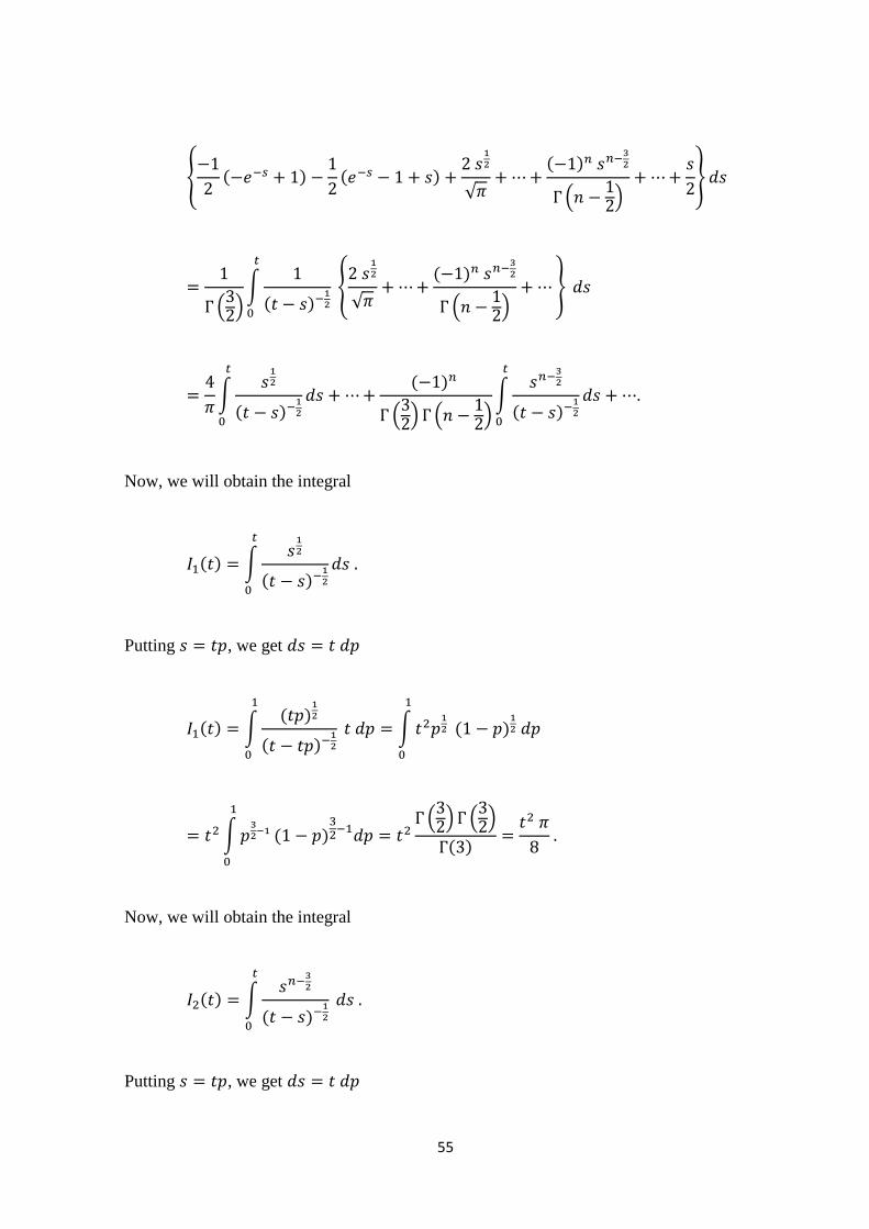
Now, we will obtain the integral
( ) ∫
( )
Putting , we get
( ) ∫( )
( )
∫
( )
∫
( )
.
/ .
/
( )
Now, we will obtain the integral
( ) ∫
( )
Putting , we get
56
( ) ∫( )
( )
∫
( )
∫ (
)
( )
.
/ .
/
.
/
.
/ .
/
( )
Therefore,
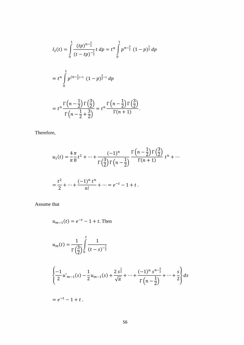
( )
( )
. / .
/
.
/ .
/
( )
( )
Assume that
( ) Then
( )
. /
∫
( )
,
( )
( )
√
( )
. /
-
57
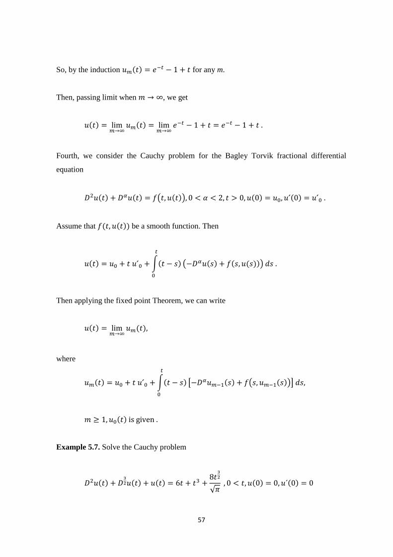
So, by the induction ( ) for any m.
Then, passing limit when , we get
( )
( )
Fourth, we consider the Cauchy problem for the Bagley Torvik fractional differential
equation
( ) ( ) ( ( )) ( ) ( )
Assume that ( ( )) be a smooth function. Then
( ) ∫( )
( ( ) ( ( )))
Then applying the fixed point Theorem, we can write
( )
( )
where
( ) ∫( )
[ ( ) ( ( ))]
( )
Example 5.7. Solve the Cauchy problem
( ) ( ) ( )
√ ( ) ( )
58
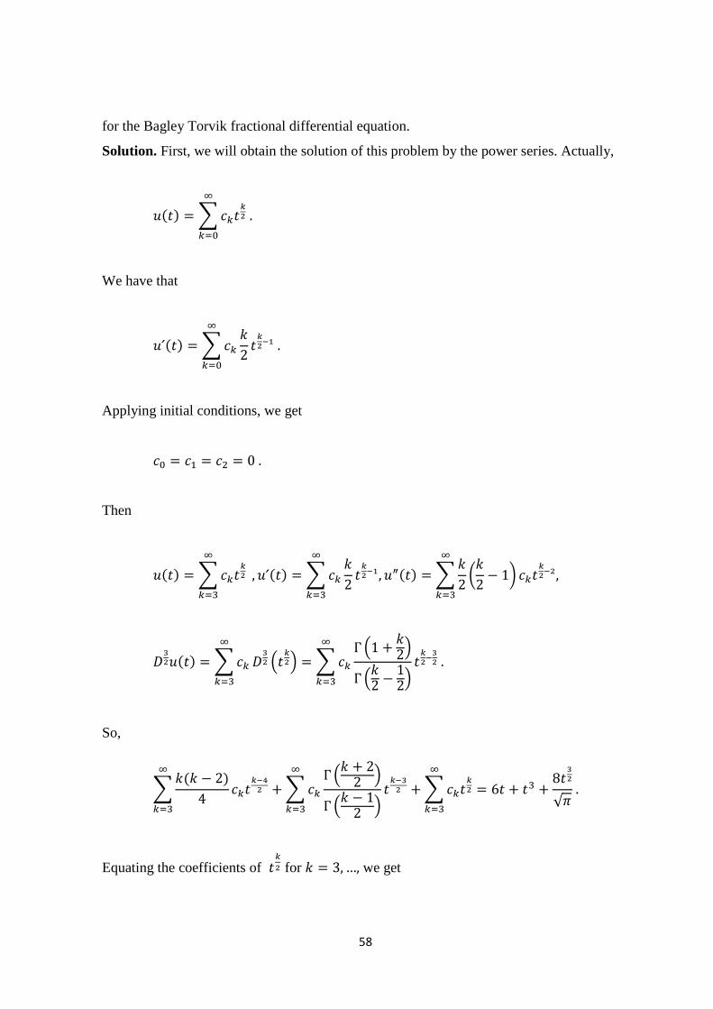
for the Bagley Torvik fractional differential equation.
Solution. First, we will obtain the solution of this problem by the power series. Actually,
( ) ∑
We have that
( ) ∑
Applying initial conditions, we get
Then
( ) ∑
( ) ∑
( ) ∑
(
)
( ) ∑
.
/ ∑
. /
.
/
So,
∑ ( )
∑
.
/
.
/
∑
√
Equating the coefficients of
for we get
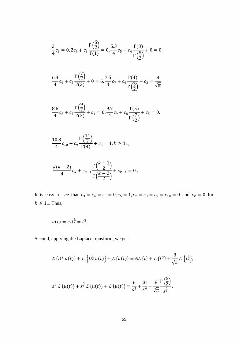
59
. /
( )
( )
. /
. /
( )
( )
. /
√
. /
( )
( )
. /
. /
( )
( )
.
/
.
/
It is easy to see that and for
Thus,
( )
Second, applying the Laplace transform, we get
* ( )+ 2 ( )3 * ( )+ * + * +
√ 2
3
* ( )+ * ( )+ * ( )+
√
. /
61
. / * ( )+
.
/
Therefore
* ( )+
( ) {
}
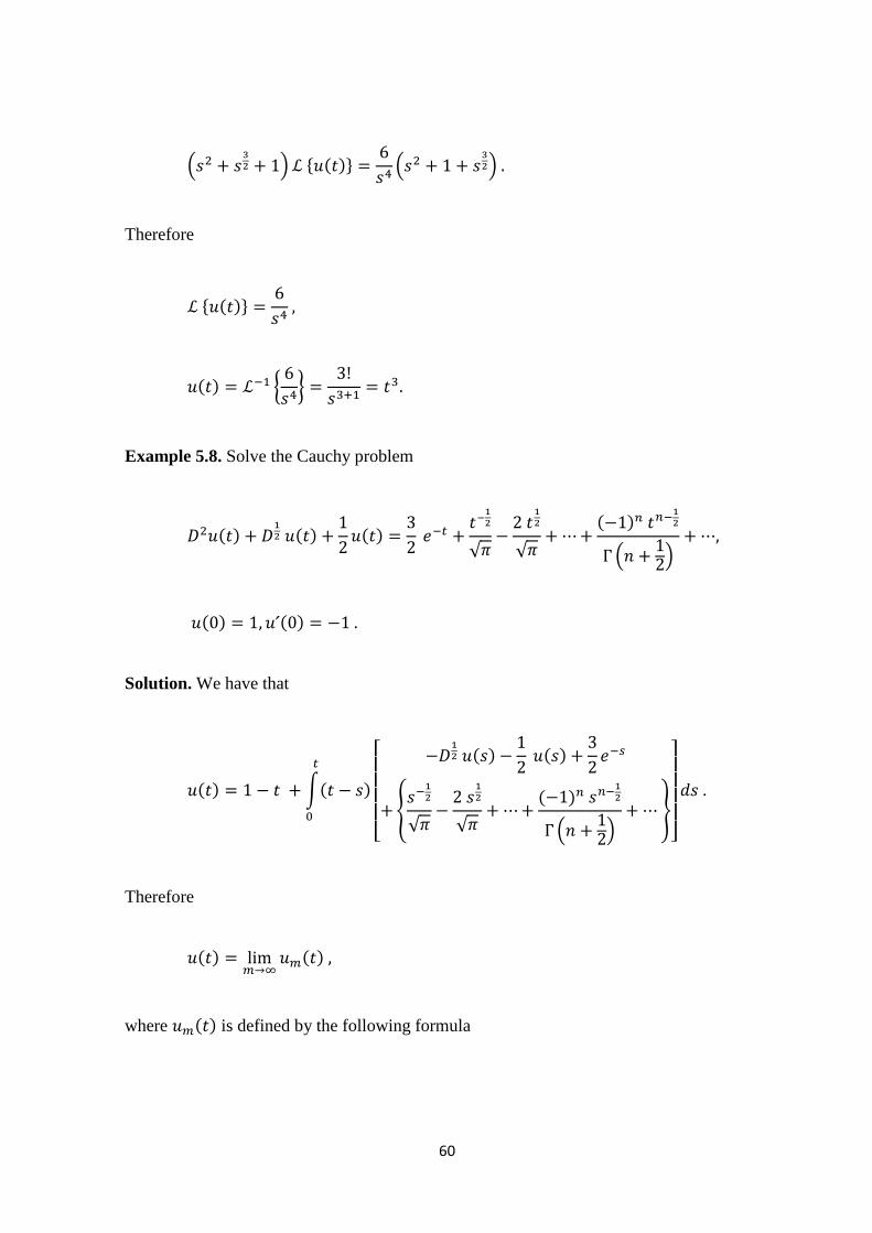
Example 5.8. Solve the Cauchy problem
( ) ( )
( )
√
√
( )
. /
( ) ( )
Solution. We have that
( ) ∫( )
[
( )
( )
,
√
√
( )
. /
-
]
Therefore
( )
( )
where ( ) is defined by the following formula
61
( ) ∫( )
[
( )
( )
,
√
√
( )
. /
-
]
( ) is given smooth function.
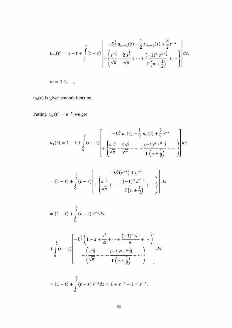
Putting ( ) we get
( ) ∫( )
[
( )
( )
,
√
√
( )
. /
-
]
( ) ∫( )
[
( )
,
√
( )
. /
-
]
( ) ∫( )
∫( )
[
4
( )
5
,
√
( )
. /
-
]
( ) ∫( )
62
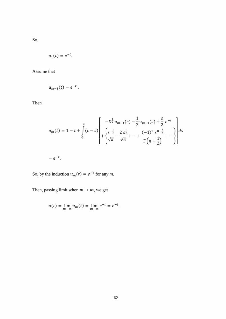
So,
( )
Assume that
( )
Then
( ) ∫( )
[
( )
( )
,
√
√
( )
. /
-
]
So, by the induction ( ) for any m.
Then, passing limit when , we get
( )
( )
63
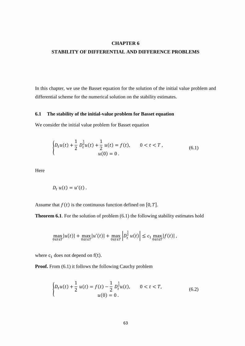
CHAPTER 6
STABILITY OF DIFFERENTIAL AND DIFFERENCE PROBLEMS
In this chapter, we use the Basset equation for the solution of the initial value problem and
differential scheme for the numerical solution on the stability estimates.
6.1 The stability of the initial-value problem for Basset equation
We consider the initial value problem for Basset equation
{ ( )
( )
( ) ( )
( ) (6.1)
Here
( ) ( )
Assume that ( ) is the continuous function defined on , -.
Theorem 6.1. For the solution of problem (6.1) the following stability estimates hold
| ( )|
| ( )|
|
( )|
| ( )|
where does not depend on ( )
Proof. From (6.1) it follows the following Cauchy problem
{ ( )
( ) ( )
( )
( ) (6.2)
64
It is a linear problem and the following formula holds
( )
( ) ∫
( )
[ ( )
( )]
∫
( )
[ ( )
( )] (6.3)
Using the last formula, we can write
( ) ( )
( )
∫
( )
[ ( )
( )] (6.4)
Using the definition of fractional derivative and formula (6.3) and (6.4), we get
( )
√ ∫
( )
( )
√ ∫
( )
{ ( )
∫
( ) ( )
}
√ ∫
( )
{
( )
∫
( )
( )
}
√ ∫
( )
{ ( )
∫
( ) ( )
}
65
√ ∫
( )
( )
√ ∫
( )
∫ ( )
( )
We denote that
( )
( ) (6.5)
Then, from the last formula it follows that
( )
√ ∫
( )
{ ( )
∫
( ) ( )
}
√ ∫
( )
( )
√ ∫
( )
∫ ( )
( ) (6.6)
First, we will consider the integral
( )
√ ∫
( )
( )
√ ∫
( )
( )
√ ∫
( )
√ ∫
( )
( )
66
Changing the order of integration and using
, - , -, we get
∫ ∫
( )
( ) ( )
∫ ∫
( ) ( )
( )
∫ ( )
( )
where
( )
∫
( ) ( )
Putting , we get and
( )
∫
( )
Putting ( ) we get ( ) and
( )
∫
( )
( )
( )
∫( )
(
)
4 . /5
( )
Then
67
( ) ∫ ( )
( )
Using formulas (6.3) and (6.5), we obtain
( )
√ ∫
( )
( )
∫
( )
[ ( )
( )] (6.7)
Second, we will estimate the double integral above
( )
√ ∫
( )
∫ ( )
( )
Changing the order of integration and using
, - , -, we get
( )
√ ∫ ∫
( )
( )
( ) ∫ ( )
( )
Were
( )
√ ∫
( )
( )
Putting , we get and
68
( )
√ ∫
( )
√ ∫
( )
√
√
√
√ (6.8)
Applying the triangle inequality, formulas (6.6), (6.7) and estimate (6.8), we get
| ( )|
√ ∫
( )
{| ( )|
∫
( )| ( )|
}
∫
( )
{| ( )|
| ( )|} ∫ ( )
| ( )|
4 √
√ 5
| ( )| ∫ 4
√
√ 5
| ( )|
Applying the integral inequality, we get
| ( )| 4 √
√ 5
| ( )|
4
√
√ 5
for any , -. From that it follows that
|
( )| 4
√
√ 5
4
√
√ 5
| ( )| (6.9)
Applying the triangle inequality and estimate (6.9), we get
69
| ( )| | ( )|
∫
( )
| ( )|
|
( )|
∫
( )
|
( )|
| ( )|
|
( )|
[ 4 √
√ 5
4
√
√ 5
]
| ( )| (6.10)
Applying the triangle inequality and estimates (6.9) and (6.10), we get
| ( )| | ( )| | ( )| |
( )|
| ( )| (6.11)
Finally, applying estimate (6.9), (6.10) and (6.11), we get
| ( )|
| ( )|
|
( )|
| ( )|
Theorem 6.1 is proved.
6.2 The stability of the difference scheme for the Basset equation
Applying the formula
( )
√ ∑
( )
∫
( )
(6.12)
71
and implicit difference scheme, we get the following difference scheme
{
( )
(6.13)
for the numerical solution of the initial value problem (6.1).
We have that
∑
[
] (6.14)
∑
[
]
where
.
/
From formula (6.14) it follows
[
]
[
]
∑
[
]
(6.15)
Theorem 6.2. For the solution of difference scheme (6.13) the following stability estimates
hold
71
| |
|
|
|
|
| | (6.16)
where does not depend on and
Proof. Applying the formulas (6.12), (6.15), we get
√ ∑
( )
∫
{ (
)
∑
(
)}
√
( ) ∫
{ (
)}
We denote that
(6.17)
Then, from the last formula it follows that
√ ∑
( )
∫
{
∑
}
√ ∑
( )
∫
{
∑
}
72
(6.17a)
where
√ ∑
( )
∫
{
∑
}
√ ∑
( )
∫
{
∑
}
√ ∑
( )
∫
* +
√ ∑
( )
∫
{
}
√ ∫
{
∑
}
√ ∫
{
∑
}
Now, we will estimate | | | | | | | | | | and | |, separately.
Applying the triangle inequality, Holder's inequality, we get
| |
√ √ ∑ ∫
( )
| |
73
√
√ ∑
√
∫( )
(( ) )
( )
(( ) )
| |
√
√ ∑
√
(∫
( )
)
(∫
( )
)
| |
√ ∑
√
√
| |
√ ∫
√
| |
√ √
| |
for any
Applying the triangle inequality, we can obtain
| |
√ ∑
. /
( )
{
∑
| |}
| |
√ ∑
. /
( )
| |
√ ∑
√
. /
√ ( )
Applying Holder's inequality, we get
. /
√ ( ) √
( ) ∫
74
√
( ) ∫
√
( ) (∫
)
(∫
)
√
( ) ( ( ))
( ( ))
√
( ) (( ) )
(( ) )
(6.18)
Therefore
| |
| |
√ ∫
√
√
√
| |
for any
Now, we will estimate | |
Applying the triangle inequality and estimate (6.18), we get
| |
√ ∑
( )
∫
{
∑ | |
}
√
√ ∑
√
{
∑ | |
}
since , - , - we have
that
75
√ ∑
√
√
{
∑ | |
}
√ ∑ √
∑
√
{ | |}
Therefore,
| | √
√
∑ | |
∑
√
√ ∑
| | ∑
√
√ ∑
| | ∫
√
√
√ ∑
| |
for any .
Now, we will estimate | |. By (6.13), we have that
| |
√ ∑
( )
∫
(
)
√
∑
( )
∫
( )
It is clear that , - , -.
Therefore, changing the order of summation, we get
76
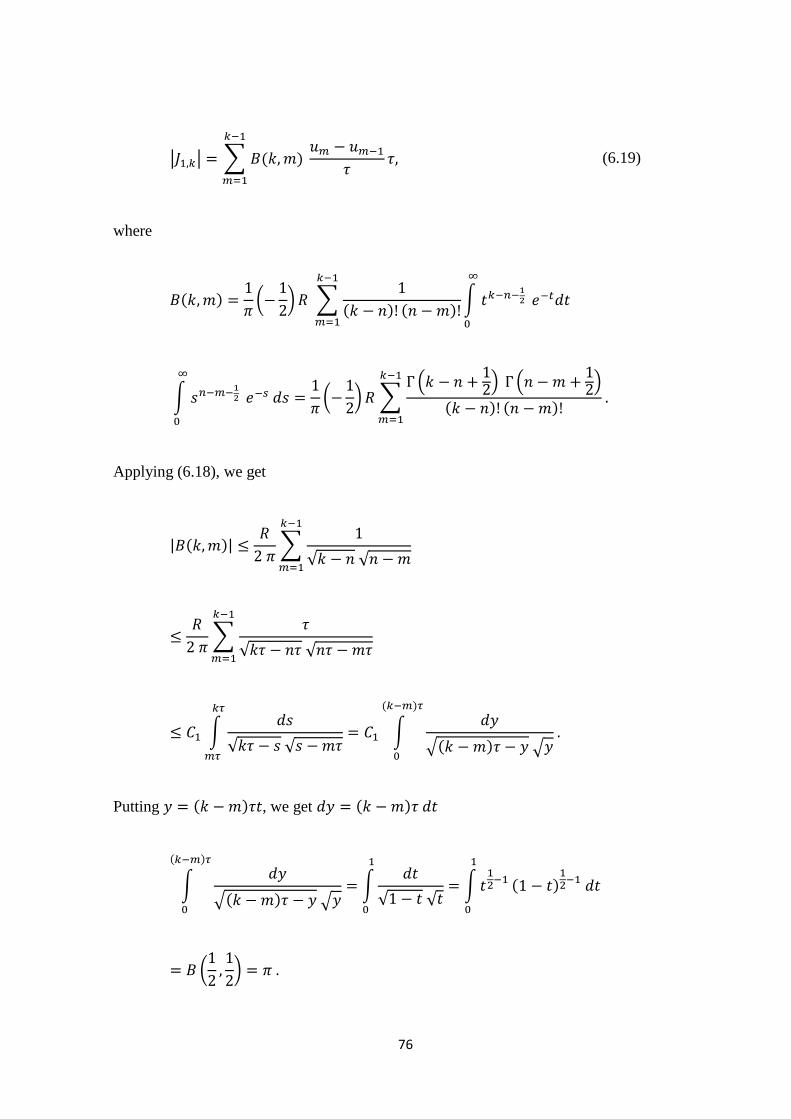
| | ∑ ( )
(6.19)
where
( )
(
) ∑
( ) ( )
∫
∫
(
) ∑
. / .
/
( ) ( )
Applying (6.18), we get
| ( )|
∑
√ √
∑
√ √
∫
√ √
∫
√( ) √
( )
Putting ( ) , we get ( )
∫
√( ) √
( )
∫
√ √
∫
( )
(
)
77
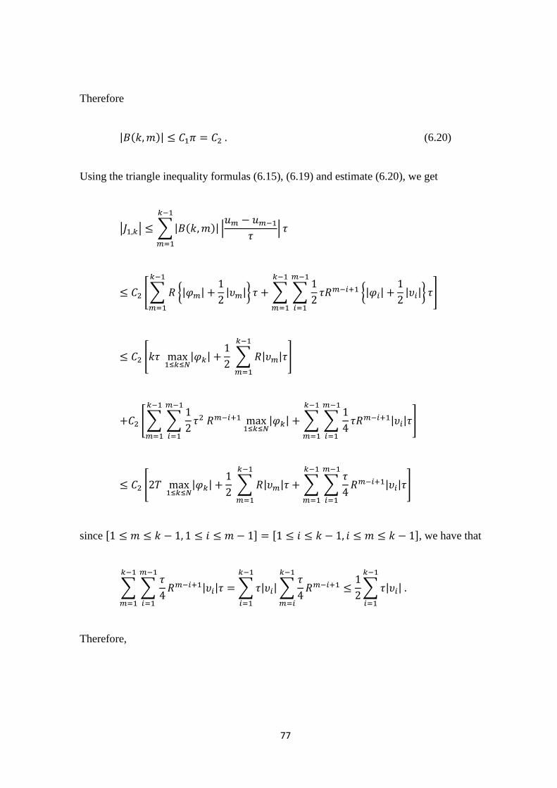
Therefore
| ( )| (6.20)
Using the triangle inequality formulas (6.15), (6.19) and estimate (6.20), we get
| | ∑ | ( )|
|
|
[∑
{| |
| |} ∑ ∑
{| |
| |} ]
[
| |
∑ | |
]
[∑ ∑
| | ∑ ∑
| | ]
[
| |
∑ | |
∑ ∑
| |
]
since , - , -, we have that
∑ ∑
| |
∑ | |
∑
∑ | |
Therefore,
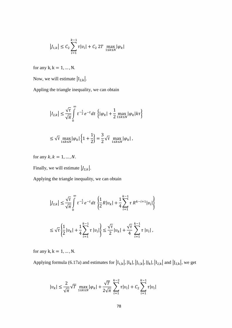
78
| | ∑ | |
| |
for any
Now, we will estimate | |.
Appling the triangle inequality, we can obtain
| | √
√ ∫
{| |
| | }
√
| | {
}
√
| |
for any
Finally, we will estimate | |.
Applying the triangle inequality, we can obtain
| | √
√ ∫
{
| |
∑ | |
}
√ {
| |
∑ | |
} √
| |
√
∑ | |
for any
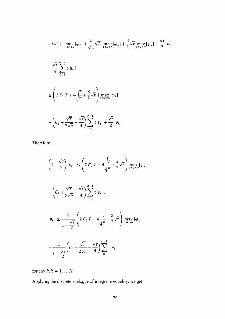
Applying formula (6.17a) and estimates for | | | | | | | | | | and | |, we get
| |
√ √
| |
√
√ ∑ | |
∑ | |
79
| |
√ √
| |
√
| |
√
| |
√
∑ | |
( √
√ )
| |
4 √
√
√
5 ∑ | |
√
| |
Therefore,
4 √
5 | | ( √
√ )
| |
4 √
√
√
5 ∑ | |
| |
√
( √
√ )
| |
√
4 √
√
√
5 ∑ | |
for any
Applying the discrete analogue of integral inequality, we get
81
| |
√
( √
√ )
| |
4 √
√
√
5
√
for any From that it follows that
|
|
√
( √
√ )
4 √
√
√
5
√
| | (6.21)
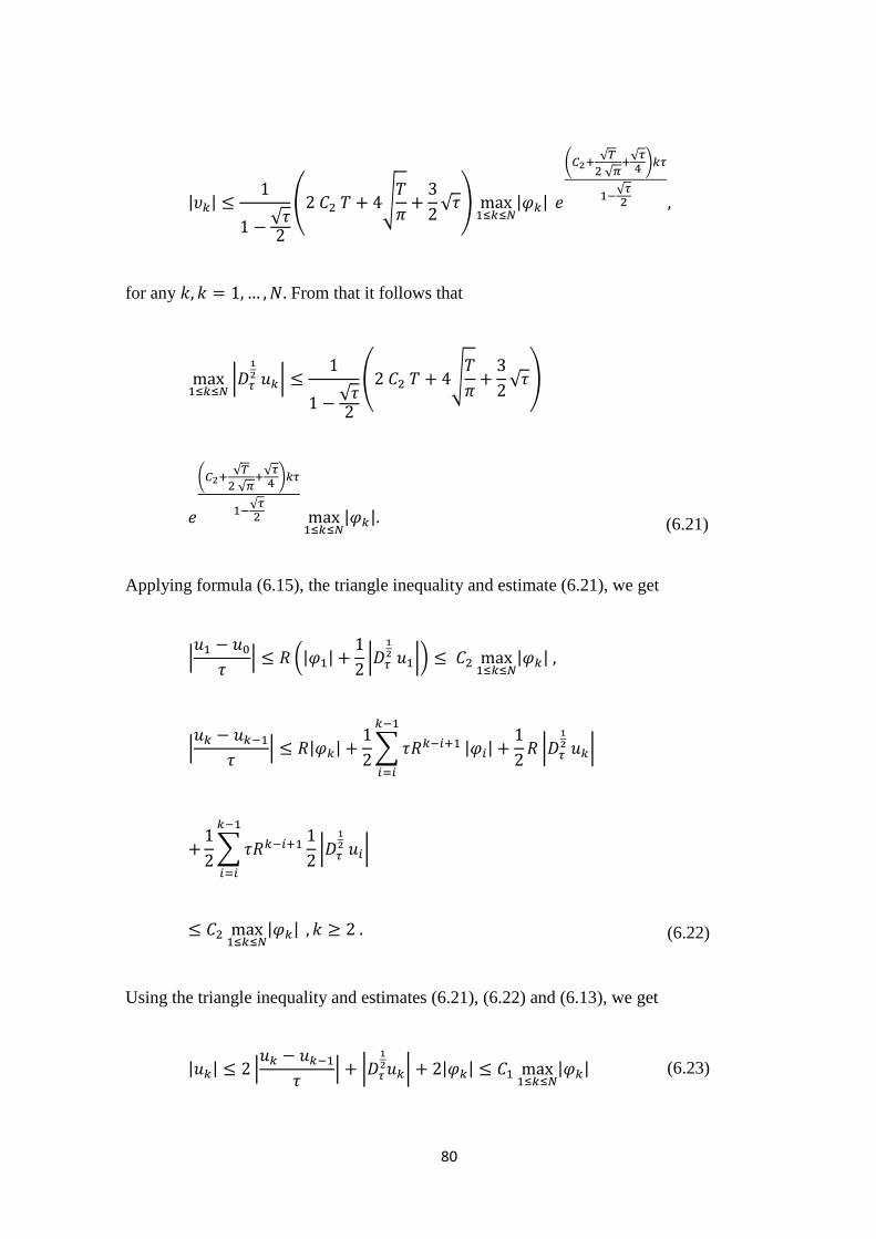
Applying formula (6.15), the triangle inequality and estimate (6.21), we get
|
| (| |
|
|)
| |
|
| | |
∑
| |
|
|
∑
|
|
| | (6.22)
Using the triangle inequality and estimates (6.21), (6.22) and (6.13), we get
| | |
| |
| | |
| | (6.23)
81
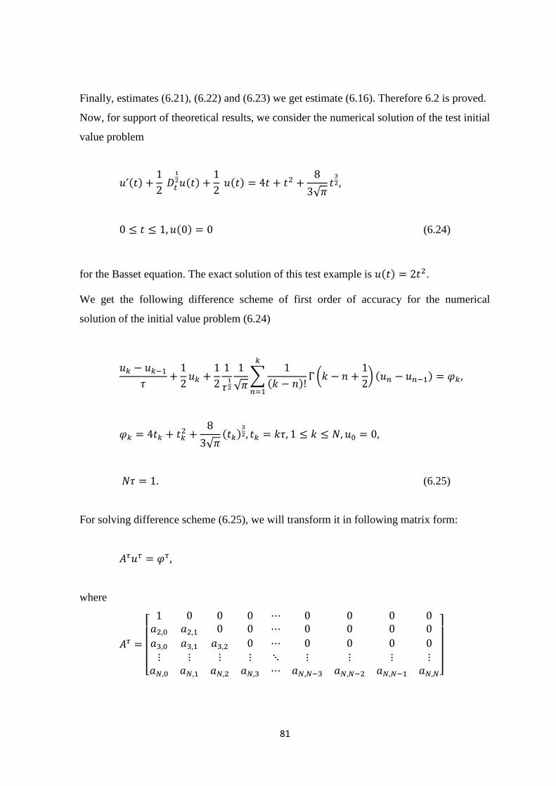
Finally, estimates (6.21), (6.22) and (6.23) we get estimate (6.16). Therefore 6.2 is proved.
Now, for support of theoretical results, we consider the numerical solution of the test initial
value problem
( )
( )
( )
√
( ) (6.24)
for the Basset equation. The exact solution of this test example is ( ) .
We get the following difference scheme of first order of accuracy for the numerical
solution of the initial value problem (6.24)
√ ∑
( )
(
) ( )
√ ( )
(6.25)
For solving difference scheme (6.25), we will transform it in following matrix form:
where
[
]
82
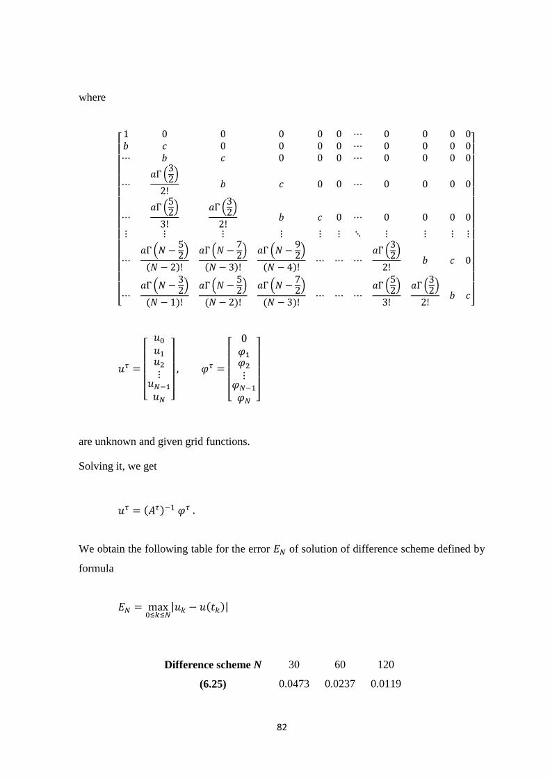
where
[
.
/
.
/
. /
.
/
( )
.
/
( )
.
/
( )
.
/
.
/
( )
. /
( )
. /
( )
. /
. /
]
[
]
[
]
are unknown and given grid functions.
Solving it, we get
( )
We obtain the following table for the error of solution of difference scheme defined by
formula
| ( )|
Difference scheme N 30 60 120
(6.25) 0.0473 0.0237 0.0119

83
As it is seen in this table, we get some numerical results. If N are doubled, the value of
errors decrease by a factor of approximately
for first order of accuracy difference
scheme.
84
CHAPTER 7
CONCLUSIONS
This work is dedicate to study fractional calculus and its applications for the fractional
Basset equation.
The following results are obtained:
Study properties of fractional integral.
Study properties of Caputo fractional differential operator.
Study properties of Riemann - Liouville fractional differential operator.
Methods for the solutions of initial value problems fractional differential
equations are applied.
The theorem on the stability estimates for the solution of the initial value problem
for the fractional Basset equation is established.
The theorem on the stability estimates for the solution of the first order of
accuracy differential scheme for the numerical solution of the initial value
problem for the fractional Basset equation is proved.
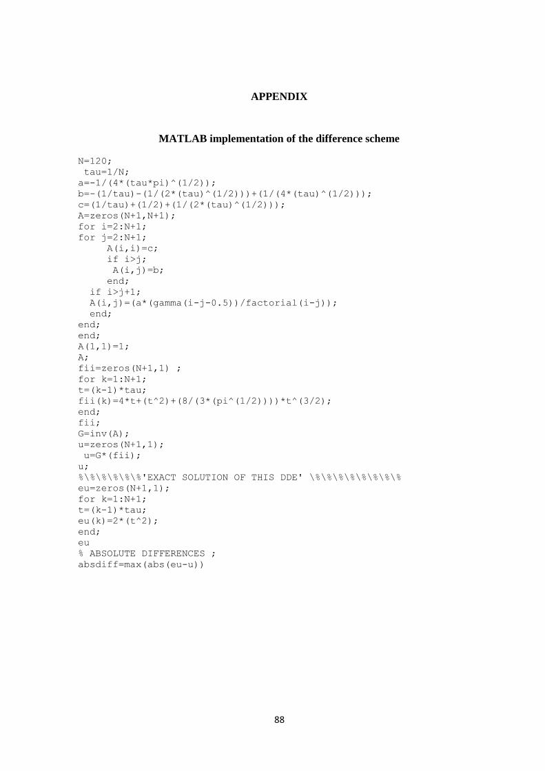
The MATLAB implementation of the difference scheme for the numerical
solution of the test Basset problem is presented.
The theoretical expressions for the solutions of the difference scheme are
supported by the results of numerical examples.
85
REFERENCES
AA Kilbas, Srivastava, H., & Trujillo, J. (2006). Theory and Applications of Fractional
Differential Equations. Amsterdam: Elsevier.
Ashyralyev, A. (2009). A note on fractional derivatives and fractional powers of operators.
Journal of Mathematical Analysis and Applications, 357(1), 232–236.
Ashyralyev, A., & Sharifov, Y. A. (2012). Existence and uniqueness of solutions for the
system of nonlinear fractional differential equations with nonlocal and integral
boundary conditions. In Abstract and Applied Analysis (Vol. 2012). Hindawi
Publishing Corporation.
Barkai, E., Metzler, R., & Klafter, J. (2000). From continuous time random walks to the
fractional Fokker-Planck equation. Physical Review E, 61(1), 132.
Benson, D. A., Wheatcraft, S. W., & Meerschaert, M. M. (2000). Application of a
fractional advection‐dispersion equation. Water Resources Research, 36(6), 1403–
1412.
Benson, D. A., Wheatcraft, S. W., & Meerschaert, M. M. (2000). The fractional‐order
governing equation of Lévy motion. Water Resources Research, 36(6), 1413–1423.
Diethelm, K. (2010). The analysis of fractional differential equations: An application-
oriented exposition using differential operators of Caputo type. Springer.
Ishteva, M. (2005). Properties and applications of the Caputo fractional operator.
Department of Mathematics, University of Karlsruhe, Karlsruhe.
Kreui, S. G. (2011). Linear differential equations in Banach space (Vol. 29). American
Mathematical Soc.
86
Liu, F., Anh, V., & Turner, I. (2004). Numerical solution of the space fractional Fokker–
Planck equation. Journal of Computational and Applied Mathematics, 166(1), 209–
219.
Lovoie, J. L., Osler, T. J., & Tremblay, R. (1976). Fractional derivatives and special
functions. SIAM Review, 18(2), 240–268.
Metzler, R., & Klafter, J. (2000). Boundary value problems for fractional diffusion
equations. Physica A: Statistical Mechanics and Its Applications, 278(1), 107–125.
Munkhammar, J. (2004). Riemann-Liouville fractional derivatives and the Taylor-Riemann
series.
Oldham, K., & Spanier, J. (1974). The fractional calculus theory and applications of
differentiation and integration to arbitrary order (Vol. 111). Elsevier.
Othman, A. R., & Mazli, M. A. M. (2012). Influences of Daylighting towards Readers’
Satisfaction at Raja Tun Uda Public Library, Shah Alam. Procedia-Social and
Behavioral Sciences, 68, 244–257. https://doi.org/10.1016/j.sbspro.2012.12.224
Podlubny, I. (1998). Fractional differential equations: an introduction to fractional
derivatives, fractional differential equations, to methods of their solution and some of
their applications (Vol. 198). Academic press.
Saichev, A. I., & Zaslavsky, G. M. (1997). Fractional kinetic equations: solutions and
applications. Chaos: An Interdisciplinary Journal of Nonlinear Science, 7(4), 753–
764.
Samko, S. G., Kilbas, A. A., & Marichev, O. I. (1993). Fractional integrals and derivatives.
Theory and Applications, Gordon and Breach, Yverdon, 1993.
Tarasov, V. E. (2007). Fractional derivative as fractional power of derivative. International
Journal of Mathematics, 18(3), 281–299.
87
Yuste, S. B., & Lindenberg, K. (2001). Subdiffusion-limited A+ A reactions. Physical
Review Letters, 87(11), 118301.
Yuste, S. B., Acedo, L., & Lindenberg, K. (2004). Reaction front in an A+ B→ C reaction-
subdiffusion process. Physical Review E, 69(3), 36126.
Zaslavsky, G. M. (2002). Chaos, fractional kinetics, and anomalous transport. Physics
Reports, 371(6), 461–580.
88
APPENDIX
MATLAB implementation of the difference scheme
N=120;
tau=1/N;
a=-1/(4*(tau*pi)^(1/2));
b=-(1/tau)-(1/(2*(tau)^(1/2)))+(1/(4*(tau)^(1/2)));
c=(1/tau)+(1/2)+(1/(2*(tau)^(1/2)));
A=zeros(N+1,N+1);
for i=2:N+1;
for j=2:N+1;
A(i,i)=c;
if i>j;
A(i,j)=b;
end;
if i>j+1;
A(i,j)=(a*(gamma(i-j-0.5))/factorial(i-j));
end;
end;
end;
A(1,1)=1;
A;
fii=zeros(N+1,1) ;
for k=1:N+1;
t=(k-1)*tau;
fii(k)=4*t+(t^2)+(8/(3*(pi^(1/2))))*t^(3/2);
end;
fii;
G=inv(A);
u=zeros(N+1,1);
u=G*(fii);
u;
%\%\%\%\%\%'EXACT SOLUTION OF THIS DDE' \%\%\%\%\%\%\%\%
eu=zeros(N+1,1);
for k=1:N+1;
t=(k-1)*tau;
eu(k)=2*(t^2);
end;
eu
% ABSOLUTE DIFFERENCES ;
absdiff=max(abs(eu-u))