Embed Size (px)
Citation preview

University of New MexicoUNM Digital Repository
Mechanical Engineering ETDs Engineering ETDs
Summer 7-15-2017
A Thermodynamic Study of Binary Real GasMixtures Undergoing Normal ShocksJosiah M. BigelowUniversity of New Mexico
Follow this and additional works at: https://digitalrepository.unm.edu/me_etds
Part of the Mechanical Engineering Commons
This Thesis is brought to you for free and open access by the Engineering ETDs at UNM Digital Repository. It has been accepted for inclusion inMechanical Engineering ETDs by an authorized administrator of UNM Digital Repository. For more information, please [email protected].
Recommended CitationBigelow, Josiah M.. "A Thermodynamic Study of Binary Real Gas Mixtures Undergoing Normal Shocks." (2017).https://digitalrepository.unm.edu/me_etds/168

Josiah Michael Bigelow
Candidate
Mechanical Engineering
Department
This thesis is approved, and it is acceptable in quality and form for publication:
Approved by the Thesis Committee:
Dr. C. Randall Truman, Chairperson
Dr. Peter Vorobieff
Dr. Timothy Clark
Dr. Humberto Silva III
A Thermodynamic Study of Binary RealGas Mixtures Undergoing Normal Shocks
by
Josiah Michael Bigelow
B.S., Mechanical Engineering, Kansas State University, 2013
THESIS
Submitted in Partial Fulfillment of the
Requirements for the Degree of
Master of Science
Mechanical Engineering
The University of New Mexico
Albuquerque, New Mexico
July, 2017
ii

Dedication
To my wife, for her perseverance, fellowship, proof reading, and encouragement
throughout this process.
“Not all who wander are lost.” – Bilbo Baggins
iii

Acknowledgments
As with any undertaking of appreciable scale and effort, the limits of who to thankare not sharply defined. I would like to take a few lines and express my gratitude, byname, to some of the most important people who have supported this project1. Myadviser, Dr. Truman, has been truly helpful and patient throughout this project,thank you for taking me on and for all of the guidance. The members of my commit-tee, Dr. Silva, Dr. Clark, and Dr. Vorobieff, have all provided insight into numericalmodeling, fun discussions, philosophical inquiry, and humorous stories about theirexperiences, thank you all. A special thanks to Dr. Silva for coadvising the numericalanalysis of this research. The time given by Dr. Michael Hobbs of Sandia NationalLaboratories in teach me how to use the TIGER code set is deeply appreciated.Dr. David Kitell, also of Sandia, provided moral support and explained how CTHworked, thank you sir! My wife, Shannon, has been a source of encouragement andsupport, as well as a patient listener while I describe how my programs work, thankyou, and congratulations on completing your masters degree as well. My family hasbeen not only supportive, but understanding that life is crazy when you live far awayand work while going to graduate school, I love you all. I would like to thank mycurrent and past managers at Sandia National Laboratories who have supported mycontinued education, Rich Graham, Abe Sego, Heather Schriner, and Nick Dereu,you all have been wonderful. Finally, I would like to thank my colleagues at Sandiawho have supported and encouraged me while I have been in school, you have madethe process of finishing much more enjoyable.
1A hearty shout out to Donald Knuth for inventing TEX
iv

A Thermodynamic Study of Binary RealGas Mixtures Undergoing Normal Shocks
by
Josiah Michael Bigelow
B.S., Mechanical Engineering, Kansas State University, 2013
M.S., Mechanical Engineering, University of New Mexico, 2017
Abstract
We investigate the difference between Amagat and Dalton mixing laws for gaseous
equations of state (EOS) using planar traveling shocks. Numerical modeling was
performed in the Sandia National Laboratories hydrocode CTH utilizing tabular
EOS in the SESAME format. Numerical results were compared to experimental
work from the University of New Mexico Shock Tube Laboratory. Latin hypercube
samples were used to assess model sensitivities to Amagat and Dalton EOS. We
find that the Amagat mixing law agrees best with the experimental results and that
significant difference exist between the predictions of the Amagat and Dalton mixing
methods.
v

Contents
List of Figures ix
List of Tables xi
Glossary xiii
1 Introduction and Theory 1
1.1 Problem Statement . . . . . . . . . . . . . . . . . . . . . . . . . . . . 1
1.2 Equation of State . . . . . . . . . . . . . . . . . . . . . . . . . . . . . 4
1.3 Numerical Analysis . . . . . . . . . . . . . . . . . . . . . . . . . . . . 5
1.4 Verification and Validation . . . . . . . . . . . . . . . . . . . . . . . . 5
2 Methodology 7
2.1 Equation of State . . . . . . . . . . . . . . . . . . . . . . . . . . . . . 7
2.1.1 EOS Model . . . . . . . . . . . . . . . . . . . . . . . . . . . . 7
2.1.2 SESAME Tables . . . . . . . . . . . . . . . . . . . . . . . . . 11
vi

Contents
2.2 Numerical Analysis . . . . . . . . . . . . . . . . . . . . . . . . . . . . 12
2.2.1 CTH . . . . . . . . . . . . . . . . . . . . . . . . . . . . . . . . 13
2.2.2 SESAME Refinement . . . . . . . . . . . . . . . . . . . . . . . 13
2.2.3 Spatial Grid . . . . . . . . . . . . . . . . . . . . . . . . . . . . 15
2.2.4 Shock Tube Modeling . . . . . . . . . . . . . . . . . . . . . . . 16
2.3 Verification and Validation . . . . . . . . . . . . . . . . . . . . . . . . 18
2.3.1 Incremental Latin Hypercubes . . . . . . . . . . . . . . . . . . 19
2.3.2 Sample Selection . . . . . . . . . . . . . . . . . . . . . . . . . 21
3 Results 25
3.1 EOS Verification . . . . . . . . . . . . . . . . . . . . . . . . . . . . . 26
3.2 Spatial Grid . . . . . . . . . . . . . . . . . . . . . . . . . . . . . . . . 27
3.3 Shock Tube Simulations . . . . . . . . . . . . . . . . . . . . . . . . . 29
3.3.1 Shock Speed, Us . . . . . . . . . . . . . . . . . . . . . . . . . . 30
3.3.2 Shock Pressure, Ps . . . . . . . . . . . . . . . . . . . . . . . . 32
3.3.3 Shock Temperature, Ts . . . . . . . . . . . . . . . . . . . . . . 34
3.4 LHS Analysis . . . . . . . . . . . . . . . . . . . . . . . . . . . . . . . 35
3.4.1 Shock Speed, Us . . . . . . . . . . . . . . . . . . . . . . . . . . 38
3.4.2 Shock Pressure, Ps . . . . . . . . . . . . . . . . . . . . . . . . 39
3.4.3 Shock Temperature, Ts . . . . . . . . . . . . . . . . . . . . . . 40
vii

Contents
4 Conclusions & Future Work 42
4.1 Conclusions . . . . . . . . . . . . . . . . . . . . . . . . . . . . . . . . 42
4.2 Future Work . . . . . . . . . . . . . . . . . . . . . . . . . . . . . . . . 43
Appendices 45
A Sample CTH Input 46
B Mesh Convergence 52
B.1 SESAME Grid Convergence . . . . . . . . . . . . . . . . . . . . . . . 52
B.2 Spatial Mesh Convergence . . . . . . . . . . . . . . . . . . . . . . . . 54
C Algorithms 60
C.1 Calculating Us . . . . . . . . . . . . . . . . . . . . . . . . . . . . . . . 60
C.2 Calculating Ps and Ts . . . . . . . . . . . . . . . . . . . . . . . . . . . 61
References 63
viii

List of Figures
2.1 Notional depiction of UNM Shock Tube [1] . . . . . . . . . . . . . . 18
2.2 Example of a Latin Square [2] . . . . . . . . . . . . . . . . . . . . . 20
3.1 Comparison of EOS Shock States via Rankine-Hugoniot Analysis . . 27
3.2 Shock Speed Versus Pressure Ratio . . . . . . . . . . . . . . . . . . 31
3.3 Shock Pressure Into Various Test Section Pressures . . . . . . . . . . 33
3.4 Shock Temperature Versus Pressure Ratio . . . . . . . . . . . . . . . 35
3.5 LHS QoI Results Run Against 1000 Samples . . . . . . . . . . . . . 36
3.6 Comparison of Amagat and Dalton LHS Results . . . . . . . . . . . 37
3.7 Overlap in Shock Speed Distributions, Covl = 0.8058 . . . . . . . . . 39
3.8 Overlap in Shock Pressure Distributions, Covl = 0.7527 . . . . . . . . 40
3.9 Overlap in Shock Temperature Distributions, Covl = 0.2902 . . . . . 41
B.1 Shock speed relative error in SESAME convergence . . . . . . . . . . 53
B.2 Shock Speed Logarithmic Error of Mesh Levels 1, 2, and 3 . . . . . . 57
B.3 Shock Pressure Logarithmic Error of Mesh Levels 1, 2, and 3 . . . . 58
ix

List of Figures
B.4 Shock Temperature Logarithmic Error of Mesh Levels 1, 2, and 3 . . 59
C.1 Tracer Pressure History for φ = 128.1 . . . . . . . . . . . . . . . . . 62
C.2 Tracer Temperature History for φ = 128.1 . . . . . . . . . . . . . . . 62
x

List of Tables
2.1 SESAME Refinement Levels . . . . . . . . . . . . . . . . . . . . . . 15
2.2 Driver and test section pressures [1] . . . . . . . . . . . . . . . . . . 15
2.3 Spatial Refinement Levels . . . . . . . . . . . . . . . . . . . . . . . . 16
2.4 Parameters to be Perturbed . . . . . . . . . . . . . . . . . . . . . . . 21
2.5 χ1 (Driver Pressure) Normal Distribution Fits . . . . . . . . . . . . 22
2.6 χ2 (Test Pressure) Triangular Distribution Fits . . . . . . . . . . . . 23
2.7 χ3 (Drive Densities) Triangular Distribution Fits . . . . . . . . . . . 24
2.8 χ4 (Test Density) Triangular Distribution Fits . . . . . . . . . . . . 24
2.9 χ5 (Helium Mass Fraction) Normal Distribution Fits . . . . . . . . . 24
3.1 Pressure Ratios . . . . . . . . . . . . . . . . . . . . . . . . . . . . . 26
3.2 Shock Speed Refinement Error . . . . . . . . . . . . . . . . . . . . . 28
3.3 Shock Pressure Refinement Error . . . . . . . . . . . . . . . . . . . . 29
3.4 Shock Temperature Refinement Error . . . . . . . . . . . . . . . . . 29
3.5 Simulation Shock Speed Error . . . . . . . . . . . . . . . . . . . . . 32
xi

List of Tables
3.6 Simulation Shock Pressure Error . . . . . . . . . . . . . . . . . . . . 34
3.7 Parameters Perturbed in LHS Study . . . . . . . . . . . . . . . . . . 36
B.1 SESAME Convergence Tests . . . . . . . . . . . . . . . . . . . . . . 53
B.2 Shock Speed Values . . . . . . . . . . . . . . . . . . . . . . . . . . . 55
B.3 Shock Pressure Values . . . . . . . . . . . . . . . . . . . . . . . . . . 56
B.4 Shock Temperature Values . . . . . . . . . . . . . . . . . . . . . . . 56
xii

Glossary
A JWL fit parameter
α BKW fit parameter
ASCII American Standard Code for Information Interchange
B JWL fit parameter
β BKW fit parameter
BCAT Bearcat, CTH EOS interrogation subroutine
BKW Becker-Kistiakowsky-Wilson (equation of state)
Covl Coefficient of overlap
χ LHS perturbation parameter
CTH Shock physics hydrocode
δ Absolute relative error, percent error
DAKOTA Design Analysis Kit for Optimization and Terascale Applications
e Specific energy
ε Error
xiii

Glossary
EOS Equation of State
ID Inner Diameter
JCZ Jacobs-Cowperthwaite-Zwisler (equation of state)
JCZS Jacobs-Cowperthwaite-Zwisler-Sandia (equation of state)
JWL Jones-Wilkins-Lee (equation of state)
k Co-volume of a gaseous component
κ BKW fit parameter
LANL Los Alamos National Laboratory
LJ Lennard-Jones
LHS Latin hypercube sample
M Molecular mass
m Mass
n Mole number
ω JWL fit parameter
P Pressure
QoI Quantity of Interest
R Universal gas constant
r Correlation coefficient or mesh refinement rate
Rg Specific gas constant
xiv

Glossary
Ri JWL fit parameter
ρ Density
S Entropy
s Specific entropy
SNL Sandia National Laboratories
SESAME Tabular Equation of State
T Temperature
θ BKW fit parameter
U Internal energy
UNM University of New Mexico
V Volume, or BKW volume ratio
v Specific volume
Vg Molar volume
w Mass fraction
X State variable
x Mole fraction
z Compressibility Factor
xv

Chapter 1
Introduction and Theory
1.1 Problem Statement
The problem of how to model mixtures of real gases presents the question of which
of the three measurable properties, pressure (P ), temperature (T ), and volume (V ),
apply to the whole mixture. Often the assumption is made that the measured tem-
perature applies to the mixture leaving P and V as the variables that are a function
of the components [3]. We know that for a pure, real gas the following relationship
holds [4]
PV = mRgTz, (1.1)
where z = z(P, T ) is the compressibility factor of the gas, m is the mass, and Rg is
the specific gas constant. From Amagat, we know that
V =N∑i=1
Vi, (1.2)
where Vi is the volume occupied by component i at the given temperature and
pressure of the mixture, otherwise known as the partial volume relation [3]. On the
1

Chapter 1. Introduction and Theory
other hand, from Dalton we find that
P =N∑i=1
Pi, (1.3)
where Pi is the pressure exerted by the ith component at the given temperature and
volume of the mixture, or the partial pressure relation [3].
The following question arises when comparing binary mixtures of gases: what model
is most accurate at predicting the thermodynamic properties of the mixture at a
given temperature and pressure? Numerous papers have been published about multi-
phase and multi-component flows [5], reacting flows, flows with arbitrary equations
of state [6], and mixtures at relatively low pressures [7]. Furthermore, papers have
been published on the behavior of the shock region using Monte Carlo methods
in binary gas mixtures and binary gas mixtures of perfect gases [8, 9]. There are
also some papers on mixtures of real gases [10, 11]. However, there is very little
available on which model (Amagat or Dalton) best applies to the case of a mixture
of non-reacting, real gases, undergoing shock conditions. One may assume from the
context of the available material that Amagat’s Law would be the natural choice but
it is not entirely clear that this is true [3, 4, 5, 1]. Furthermore, both models are
approximations and themselves have pressure and temperature ranges over which
they may be considered accurate [3].
The aforementioned data and references indicate that there has not been much re-
search into the specific question of mixtures of real gases under shock conditions.
This raises the following questions:
a. What thermodynamic model best describes a mixture of binary real gases un-
dergoing shocks?
b. How sensitive are the mathematical models and their numerical analogues to
perturbation?
2

Chapter 1. Introduction and Theory
Shock waves are present in many engineering applications ranging from pneumatic
systems to detonation of high explosives [1, 12]. On this spectrum applications
range from fluid-particle transport to supersonic flight of spacecraft that experience
atmospheric reentry. Often, the experiments needed to study a full system are cost
prohibitive, time consuming, or both. One way to select a design path is to nu-
merically model the system with appropriate boundary conditions. However, the
problem of closure to the governing equations (mass, momentum, and energy) re-
quires good representations of material properties. This is where a shock tube can
provide value. The thermodynamic properties of a gas or gases can be studied under
carefully controlled shock states allowing for first principles or semi-empirical models
to be refined. Methods of converting a problem to a numerical representation are
the ‘other side of the coin’ so to speak. This is where the question of how mixing is
handled when using anything other than a pure gas comes in. Does the formula used
to predict mixture behavior matter numerically? How can one build an accurate
validation space for the numerical method employed? If one were to model a set of
shocks that were impossible to reproduce in an available shock tube, how would one
have confidence in the numerical answers calculated? These and other questions led
to the genesis of this thesis. Not every question will be fully answered, but at the
core the question of mixing will be addressed.
The following problem statement is proposed to begin to attempt to answer the
questions posed above:
Model mixtures of He and SF6 in a shock tube configuration using the Sandia
National Laboratories (SNL) hydrocode CTH, utilizing SESAME table equations of
state to model Amagat, Dalton, and real behaviors. Investigate model sensitivities
to numerical methods, data uncertainty, modeling assumptions, and mixing ratios.
Where possible, match the CTH predictions to existing experimental data.
This statement of the problem will explore the relationship of the outputs of the code
3

Chapter 1. Introduction and Theory
to the inputs in a rigorous and systematic way. Verification of the outputs against
experimental data will provide a means to assess whether the choice of mixing model
matters.
1.2 Equation of State
Equations of state (EOS) are used for closure of the system of thermodynamic equa-
tions describing a process. Conservation of mass, balance of momentum, and conser-
vation of energy require a relationship that describes the thermodynamics of what
are called state variables. Often the state variables used are ones that are easily
measured experimentally such as P , T , and V . However, this need not always be
the case, because one could also construct an equation of state in terms of variables
like entropy, S, and internal energy, U , which are impossible to directly measure
experimentally [13]. Equations of state are difficult to construct entirely from first
principles with the constraint that they also be perfectly accurate for all physical
phases of a material. The ideal gas equation is an example of one such equation that
works well at describing the nature of many different gases, provided the density is
not too high. For example, if the modeled gas begins to condense the latent heat of
vaporization and the change in density from compressible to incompressible fluid are
not captured in the ideal gas model. In engineering modeling, equations of state are
often curve fits to experimental data that are semi-empirical in nature. Parts of the
equation of state are known from fundamental physics and other parts are “fit” to
improve the results of the equation(s) over a particular range of states [4, 13]. For
this problem EOS selection considered gaseous states of Helium (He) and SF6 in a
shock region since phase change was not part of the problem.
4

Chapter 1. Introduction and Theory
1.3 Numerical Analysis
Shock modeling is inherently difficult in a numerical sense [14]. Great care is required
to make codes stable and accurate across the shock since a shock is often represented
as a discontinuous jump state, introducing a cusp into the numerical results often
leading to numerical instability [14]. This research is interested in differences that
may be present in mixing formulations but not what is happening inside of the shock.
The primary interest is in the effect of the shock front as it passes through the gas
mixture. Any numerical algorithm utilized need only accurately represent the shock
effects, e.g., shock speed, shock pressure, and shock temperature, but does not need
to provide an accurate representation of the shock width or interior structure.
1.4 Verification and Validation
Verification and validation are distinct and important aspects of any numerical anal-
ysis. Verification can be thought of as checking that the correct physical models or
theories were applied. Have the governing equations been satisfied, was the mathe-
matical analysis performed correctly? Verification is an objective measure since there
are clear correct and incorrect applications of a physical law or principle. However,
validation is harder to achieve. Assumptions, numerical error, algorithm choice, etc.
all play into the validity of observed numerical results. Validation requires carefully
analyzing the process and also performing studies on model sensitivity. Generating
a validation space requires objective as well as subjective judgment about mesh re-
finement, statistics, and numerical methods. For this research, verification takes the
form of using codes that are known to provide good shock state results and accurately
model EOS. Rankine-Hugoniot analysis provided certainty that EOS surfaces passed
through the correct thermodynamic states. Validation came through comparison to
5

Chapter 1. Introduction and Theory
experimental values and exercising models via Latin hypercube sampling.
6

Chapter 2
Methodology
2.1 Equation of State
Numerical analogues to an analytic EOS were implemented in the form of SESAME
tables. This section discusses EOS engineering models considered, selection criteria,
and mixture table creation.
2.1.1 EOS Model
Four different equation of state models were considered for this research, and are in
ascending order of complexity, Ideal Gas [15], Becker-Kistiakowsky-Wilson (BKW)
[16], Jones-Wilkins-Lee (JWL) [17, 18], and Jacobs-Cowperthwaite-Zwisler (JCZ)
[19, 20]. The Ideal Gas model has promise for relatively weak shocks since the
density does not get very large. However, the stronger the shock, the worse the Ideal
Gas model will perform. The ideal gas, JWL, and BKW models were discarded after
some consideration due to questions regarding accuracy and the fact that they have
been superseded by the JCZ equations of state [20].
7
Chapter 2. Methodology
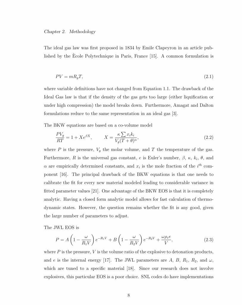
The ideal gas law was first proposed in 1834 by Emile Clapeyron in an article pub-
lished by the Ecole Polytechnique in Paris, France [15]. A common formulation is
PV = mRgT, (2.1)
where variable definitions have not changed from Equation 1.1. The drawback of the
Ideal Gas law is that if the density of the gas gets too large (either liquification or
under high compression) the model breaks down. Furthermore, Amagat and Dalton
formulations reduce to the same representation in an ideal gas [3].
The BKW equations are based on a co-volume model
PVgRT
= 1 +XeβX , X =κ∑xiki
Vg(T + θ)α, (2.2)
where P is the pressure, Vg the molar volume, and T the temperature of the gas.
Furthermore, R is the universal gas constant, e is Euler’s number, β, κ, ki, θ, and
α are empirically determined constants, and xi is the mole fraction of the ith com-
ponent [16]. The principal drawback of the BKW equations is that one needs to
calibrate the fit for every new material modeled leading to considerable variance in
fitted parameter values [21]. One advantage of the BKW EOS is that it is completely
analytic. Having a closed form analytic model allows for fast calculation of thermo-
dynamic states. However, the question remains whether the fit is any good, given
the large number of parameters to adjust.
The JWL EOS is
P = A
(1− ω
R1V
)e−R1V +B
(1− ω
R2V
)e−R2V +
ωρee
V, (2.3)
where P is the pressure, V is the volume ratio of the explosive to detonation products,
and e is the internal energy [17]. The JWL parameters are A, B, R1, R2, and ω,
which are tuned to a specific material [18]. Since our research does not involve
explosives, this particular EOS is a poor choice. SNL codes do have implementations
8

Chapter 2. Methodology
of JWL, but this EOS is particularly tuned to solid explosives that burn to produce
gaseous and condensed products [22]. The properties predicted are predicated on
line integrals along adiabatic expansion paths from an initial high temperature and
pressure state, and so would not necessarily be suited to a room temperature starting
condition [22].
The Jacobs-Cowperthwaite-Zwisler (JCZ) EOS was originally developed to give a
more general representation over a wide range of material densities [19]. SNL up-
dated the original TIGER [19] code and JCZ EOS with improved fits over ionization
ranges and additional molecular species in what is now called the JCZS EOS [12, 20].
Originally, JCZ variants were denoted by a number (e.g., JCZ2, JCZ3) allowing for
user selection when running the codes [19]. With the advent of more powerful com-
puters, selection between versions is not a necessity and the EOS is referred to as
JCZ and JCZS to differentiate between the legacy code and the SNL version [20].
The JCZ3 EOS [19] is given by
P =G(V, T )nRT
V+ P0(V ), (2.4)
where P , n, R, T , and V represent the pressure, number of moles, universal gas
constant, temperature, and volume, respectively. The Gruneisen function, G, and
internal pressure function, P0, are [20]
G = 1− V
f
(∂f
∂V
)T
; P0 = −dE0
dV, (2.5)
where f is a function based on Helmholtz free energy that ensures continuous behav-
ior across a wide range of densities and E0 is the volume potential of a face-centered
cubic lattice [19]. One can see that Equation 2.4 has a form similar to an Ideal
Gas with some correction factors. Hobbs et al. [12] updated the original Gruneisen
function to depend on a molecular potential function, EXP6, which is similar in form
to the Lennard-Jones (LJ) potential [12]. Thus, the Gruneisen function in the JCZS
9

Chapter 2. Methodology
EOS
P =G(V, T, φ)nRT
V+ P0(V, φ) (2.6)
is based on the EXP6 function
φ(r) = ε
[(6
η − 6
)eη(1−r/r
∗) −(
η
η − 6
)(r∗
r
)6]. (2.7)
Variable η is a fit parameter which has been shown to affect the EXP6 potential
relatively little [12, 20]. Due to the insensitivity of the EXP6 potential to η, most
implementations use η ≈ 13 [12]. The parameters r∗ and ε are the molecular dis-
tance of separation at the minimum potential energy and well depth for the pair
potential, respectively. The variable r is the distance by which the molecules are
separated. The advantage of ε and r∗ is that they can be calculated accurately
from generally well characterized quantities, such as the heat of formation, molecu-
lar number, and composition. Having only two parameters to calculate makes the
JCZS EOS ideal for use on a wide variety of gases [12]. The drawback of the JCZS
EOS is that, while closed form, the equations require numerical differentiation and
integration to compute thermodynamic states. Thus a dedicated code is required
to compute the thermodynamic states desired. The JCZS EOS has been shown to
provide very accurate fits to more than 750 gaseous species available through the
JANNAF (Joint Army Navy NASA Air Force Interagency Propulsion Committee)
tables demonstrating model efficacy across large variations in density and tempera-
ture [12]. Furthermore, a model parameter optimization study (sensitivity to η, r∗,
and ε) across all gaseous species for densities ranging from liquids to rarified gases
was performed [12, 20]. This verification work makes the JCZS equations ideal for
use in constructing a set of high quality tabular thermodynamic states [12, 20].
10

Chapter 2. Methodology
2.1.2 SESAME Tables
The SESAME format of tabular EOS, developed by Los Alamos National Labora-
tory (LANL) is a flexible EOS format allowing custom table generation [23]. The
TIGER code set was utilized to generate the SESAME tables for the simulations by
computing equilibrium thermodynamic states over a range of temperatures and vol-
umes representing tabular mixing for Amagat or Dalton mixtures. Construction of
a mixed EOS was performed by using MATLAB scripts taking outputs of a TIGER
data run from each pure gas and summing over either the volumes (Amagat) or the
pressures (Dalton) from each pure gas to create a single table. Two nuances to this
process are worth mentioning. Firstly, Equation 1.2 for the Amagat model is pre-
sented with volume as an extensive parameter. When summing specific volumes (an
intensive parameter) sums must be weighted by mass fraction
v(T, P ) =∑i
wivi(T, P ), (2.8)
where wi = mi
mtotis the ith mass fraction, mi is the ith mass, and mtot is the mix-
ture total mass. Similarly, specific energy in TIGER is represented as an intensive
parameter with respect to mass and is most easily summed in a mass weighted-
fashion. Secondly, since specific volume is an intensive parameter, a scaling must
be performed for the Dalton table. Given that the temperature and volume are the
independent parameters in a Dalton mixing scheme, equivalence of state is required
to get an accurate representation of the mixed pressure state. For equivalence to
occur, the volumes must be equalized. Recall that
V = mv = Mnv, (2.9)
where M is molecular mass. In the case of Dalton, we are considering partial pressure
of each constituent at the given temperature and volume. In other words, Pi =
P (T, V ). However, we have Pi = P (T, vi), which is equivalent, but not identical in
11

Chapter 2. Methodology
the sense that V 6= v. In order to sum over the He and SF6 pressures for a Dalton
formulation, we must demand that both pure He and SF6 tables represent the same
(T, v) states. The way to achieve this is to scale the specific volume of either the He
or SF6. Taking Equation 2.9 we can formulate a scaling factor for He volumes like
so
mHevHe = V = mSF6vSF6 ⇒ vHe = vSF6
mSF6
mHe
. (2.10)
The process used was to generate SF6 states in TIGER and use T and scaled v values
to generate the He states. The column of volume values for the He input was simply
scaled as shown in Equation 2.10. A simple summation of the computed He pressures
with the SF6 pressure values at each (T, v) state was then performed.
Binary SESAME files were generated by pre-processing an input deck of the de-
sired (T, V ), or (T, P ), states in MATLAB from which TIGER would calculate the
temperature (T ), pressure (P ), specific volume (v), specific energy (e), and specific
entropy (s) in that order. The resulting ASCII file was fed into the BCAT post
processor within CTH, which would generate the binary file required by CTH to run
the simulation with the tabular EOS. Thermodynamic states were selected based on
a desire for the tables to be as general as possible without growing too large to be
handled within the CTH memory constraints.
2.2 Numerical Analysis
Numerical models were developed and run in the SNL hydrocode CTH. This section
discusses CTH numerical algorithms, refinement of the SESAME tables, analysis of
the spatial grid, and models of the shock tube.
12

Chapter 2. Methodology
2.2.1 CTH
CTH was selected because it is a code that is written to study shock physics with the
ability to input tabular EOS, allowing for the study of variations in customized EOS
formulations [14]. The CTH solution scheme is a two step Eulerian method where
the mesh first deforms with the material in a Lagrangian sense and then is mapped
back to the original Eulerian positions [14]. There are six mesh options in CTH, 1D
rectangular, cylindrical, and spherical coordinates, 2D rectangular and cylindrical,
and 3D rectangular coordinates [14]. CTH implements the SESAME tabular EOS
format in the form of binary files [14, 23].
CTH contains a set of subroutines in the BCAT module that allows for Rankine-
Hugoniot analysis with a given EOS model. This permitted a study of the TIGER,
Amagat, Dalton, and Ideal Gas cases. Experimental shock pressures were plotted
as a function of shock speed with their corresponding error bars for direct EOS
comparison [1]. The various EOS models were then interrogated to see if the shock
speeds resulted in shock pressures comparable to the experimental results. This
served as a check to the validity of the EOS surfaces. If a generated table could not
replicate the experimental results that was indication of either an error in the table
generation or inability of the EOS model to accurately resolve the shock states in
the experiment. After eliminating sources of generation error, the analysis informed
the user if the EOS model was useful for this problem. Furthermore, this analysis
would quickly inform the user of differences and trends in the mixing models.
2.2.2 SESAME Refinement
When using a discrete representation of a continuous curve or surface the careful
analyst will perform a refinement study to determine sufficient numerical resolution.
Refinements to the SESAME table were handled on a basis of levels. A level describes
13

Chapter 2. Methodology
how small ∆T , ∆v, or ∆P are. Refinement means to reduce the size of the step
between temperatures, volumes, or pressures. The first level is the coarsest level
with each level above it representing a halving of ∆X; X being the thermodynamic
state variable of interest. For the first level, the number of thermodynamic states
is computed by setting the minimum, maximum, and step size values of the state
variable X using
Ni =Xmax −Xmin
∆X i
+ 1, (2.11)
where Ni is the number of values at the ith level. The number of points for each
variable was doubled every refinement step. Thus Equation 2.11 was rearranged to
compute the step size, ∆Xi+1 required to double the number of values
∆X i+1 =Xmax −Xmin
2Ni − 1. (2.12)
Since X represents temperature and then volume, respectively, the density of points
on the (T, v) surface would increase by a factor of four, for a 2D problem, with
every subsequent refinement level. From ideal gas calculations the maximum shock
temperature was found to be around 850 K. A SESAME table was generated with
TIGER performing the mixing to estimate mixture defect from ideal behavior and
help set bounds on T , v, and P . The pure He and SF6 tables were generated for both
the Amagat and Dalton mixtures. In order to provide some bound that could account
for higher pressures or temperatures, Tmax = 1500 K was selected. Correspondingly
Tmin = 180 K was chosen for the lower temperature bound. Similarly vmax = 6005
cc/g and vmin = 5 cc/g were chosen for the mixture. The initial values of ∆T and
∆v were picked to provide relatively coarse spacing without being so large that many
refinement levels were required for convergence. The maximum and minimum values
of each property were held fixed to provide the proper refinement sequence. Table 2.1
shows the details of the first three refinements for the SESAME files. A convergence
study was performed on the SESAME tables by holding the initial conditions and
spatial mesh constant in 12 different shock tube configurations studied by Trueba
14
Chapter 2. Methodology
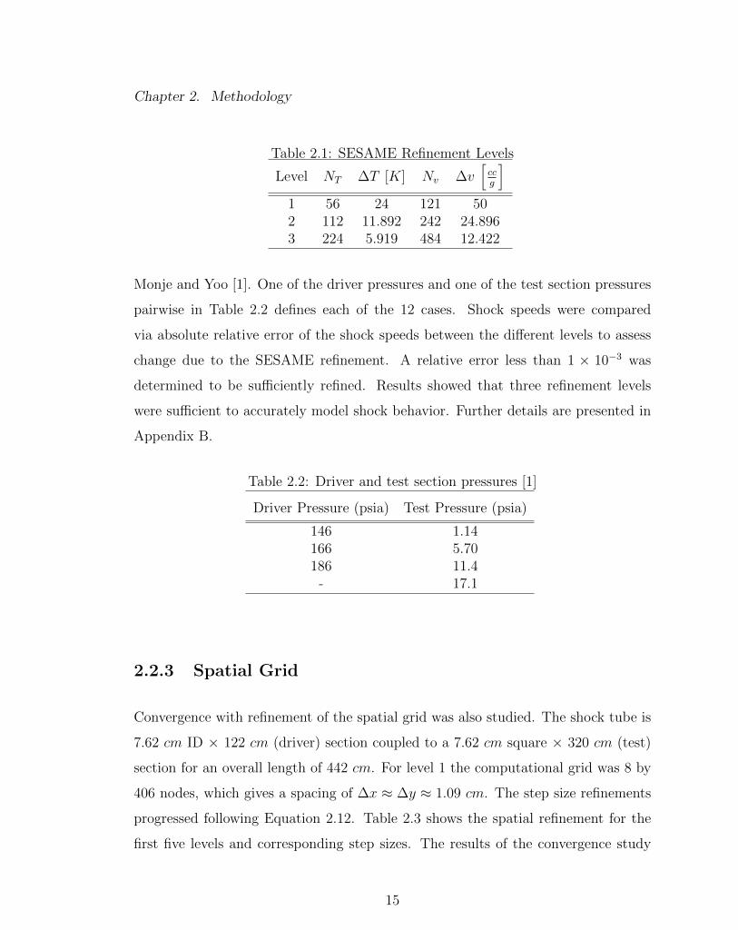
Table 2.1: SESAME Refinement Levels
Level NT ∆T [K] Nv ∆v[ccg
]1 56 24 121 502 112 11.892 242 24.8963 224 5.919 484 12.422
Monje and Yoo [1]. One of the driver pressures and one of the test section pressures
pairwise in Table 2.2 defines each of the 12 cases. Shock speeds were compared
via absolute relative error of the shock speeds between the different levels to assess
change due to the SESAME refinement. A relative error less than 1 × 10⁻³ was
determined to be sufficiently refined. Results showed that three refinement levels
were sufficient to accurately model shock behavior. Further details are presented in
Appendix B.
Table 2.2: Driver and test section pressures [1]
Driver Pressure (psia) Test Pressure (psia)
146 1.14166 5.70186 11.4
- 17.1
2.2.3 Spatial Grid
Convergence with refinement of the spatial grid was also studied. The shock tube is
7.62 cm ID × 122 cm (driver) section coupled to a 7.62 cm square × 320 cm (test)
section for an overall length of 442 cm. For level 1 the computational grid was 8 by
406 nodes, which gives a spacing of ∆x ≈ ∆y ≈ 1.09 cm. The step size refinements
progressed following Equation 2.12. Table 2.3 shows the spatial refinement for the
first five levels and corresponding step sizes. The results of the convergence study
15

Chapter 2. Methodology
are detailed in Appendix B. Methods detailed in Roache were used to estimate the
convergence of the solution with mesh refinement [24]. Modeling the tube with a level
3 refinement took considerably longer to run but did not change the error much. A
level 4 refinement was not run but a level 5 refinement was performed for all cases.
This thesis bases its error estimates off of level 3 grids for reasons discussed below.
Simulation error to experiment was generally within single digit percentage points
however a few cases were approximately 15%. A few cases were run in 3D and
took quite some time to run. These cases showed significant reductions in error are
realized when modeling the tube in 3D. The 3D cases were only run with a level 1
grid and showed improvement of the error from approximately 15% to less than 5%.
Using a level 1 3D grid takes longer than using a refined 2D grid and was impractical
for the verification and validation section of this project. The choice was made to
use a 2D mesh and accept the larger error.
Table 2.3: Spatial Refinement Levels
Level Nh ∆y [cm] NL ∆x [cm]
1 8 1.089 406 1.0912 16 0.508 812 0.5453 32 0.2458 1624 0.27234 64 0.1210 3248 0.13615 128 0.0600 6496 0.0681
2.2.4 Shock Tube Modeling
CTH models were designed to study experiments performed in the shock tube at the
University of New Mexico (UNM) with a mixture of He and SF6 [1]. The availability
of this experimental data allows the numerical simulations to be validated. An
input deck was written to capture the geometry of the UNM shock tube in both
1D and 2D configurations. Limited preliminary simulations were run in 3D and
16

Chapter 2. Methodology
the results more closely matched the experimental results. However, 3D simulations
did not change the trends observed between Amagat or Dalton and would not have
changed any conclusions drawn from the 2D simulations. Simulations in 3D take
significantly longer to run and were unfeasible for Latin hypercube sample (LHS)
analysis. Furthermore, since the trends did not change between 2D and 3D, a suite
of 3D simulations was deemed unnecessary for an LHS study. A schematic image of
the shock tube is provided with dimensions in Figure 2.1. Driver and test section
pressures are listed in Table 2.2 and define 12 combinations pairwise. The UNM
shock tube is a 7.62 cm ID round steel tube coupled to a 7.62 cm square steel tube.
The round tube is the high pressure or driver section, the square tube comprises the
low pressure or test section. The driver section is separated from the test section
via a membrane, which is punctured by a pneumatically-driven broadhead arrow
head on the axis of the driver section [1]. When the membrane is punctured the
gas flow due to pressure imbalance produces a traveling planar shock wave. The
test section can be easily modified to allow for pressure transducers, thermocouples,
viewing windows, etc. due to its square shape (the sides are flat).
The shock wave produces a pressure and temperature spike as it passes through the
test section [25]. Precise spacing of the pressure transducers allows for measurement
of both the shock over-pressure and shock speed. The numerical model captures the
center-line of the tube in the transverse direction in the 2D and 1D cases; thus the
transition from round to square tubing is not modeled. The pressure transducers
are replicated by tracers in CTH at the locations of the pressure transducers in the
experiment allowing for a replication of the measurements made in the experiments.
The membrane was not modeled, but assumed to vanish when it ruptured. Thus
gases in the driver and test sections on either side at their respective pressures and
densities were placed in contact at rupture. Just as in the experiment, in the sim-
ulation a shock was formed by the high-pressure gas moving into the low-pressure
He-SF6 mixture. The walls of the tube were implemented via a reflecting boundary
17

Chapter 2. Methodology
condition on 2, 4, or 6 sides depending on whether the simulation was 1D, 2D, or 3D
respectively.
pressure after shock wave. The velocity of the shock wave calculated as the slope of the straight line (Eqn. 2)resulting from fitting the locations of the pressure transducers against the time between the pressure pulses.The distances between the pressure transducers are 0.7112 m, 0.9779 m, and 0.7112 m, respectively.
φ =p2p1
(1)
u =d l
d t(2)
Figure 1. Representation of the horizontal Shock Tube Facility at UNM. Flow direction is from left to right.
A. Experimental Procedure
The governing variables of this experiment are the initial pressures in the driver (pburst) and driven (p1)sections as well as the initial temperature (T1). In each experiment, voltage (V ) (corresponding to pressure)and time measurements were recorded by each pressure transducer, an example is shown in Fig. 2 a. Thesemeasurements were then exported to MATLAB and smoothed by using the LOWESS (locally weightedscatterplot smoothing) method in order to get rid of random noise, such as vibrations in the piezoelectriccrystals used in the pressure transducers stemming from the impulsive acceleration created by the shockwave. The filtered data was then fitted using a spline in order to get a set of continuous rather than discretevalues, an example is shown in Fig. 2 b. In this figure, the red cross represents the shock impact. This pointis used as the reference for the time measurement of each channel and is obtained as the first recordingwhose value for voltage is greater than a specified threshold (0.3 V). This threshold value is used to get thetime measurement since the shock wave, as it passes, creates a sudden increase in pressure which produces aproportional signal in the voltage output from the oscilloscope. Once the threshold was set, two boundarieswere chosen based on observation by sight, represented by green and blue crosses. The voltage correspondingto the pressure after the shock (V2) was calculated as the mean of all the values within the range specified bythese two bounds. Following the same procedure, the value for voltage before the shock (V1) was calculatedas well. Once V2 and V1 were found, it was necessary to convert the voltage measurements into the variableof interest, pressure. Calibration data were provided by the manufacturer (PCB Piezotronics) in the form ofcalibration curves, these functions were used to relate specific increases in voltage to increases in pressure.Temperature measurements were not collected, due to a lack of commercial instrumentation with a responsetime on the order of tens of microseconds. Having these measurements would have produced a considerableincrease in results reliability since two variables would have been available for comparison.
B. Uncertainty Analysis
In order to validate the experimental data and to compare with theoretical results using Dalton’s andAmagat’s Law, it is necessary to perform an uncertainty analysis. Uncertainty analysis is a useful andessential part of an experimental program.5 In this case, pressure ratio (φ) measurements will be used tocompare to theoretical values. The pressure measurements will be considered to contain several uncertaintycomponents. The uncertainty generated from each of these components will be studied individually in orderto obtain an overall evaluation of the measurement uncertainty.
In an experiment, a measurement can be expressed as a function of different independent variables givenby:
r = r(X1, X2, ......, XN ) (3)
3 of 11
American Institute of Aeronautics and Astronautics
Figure 2.1: Notional depiction of UNM Shock Tube [1]
The tube was modeled with the EOS of the gas mixture as an ideal gas as well as
using SESAME tables. CTH has a built-in implementation of the ideal gas relation
where the user provides values for cv and γ− 1, the specific heat at constant volume
and ratio of specific heats minus one, respectively [26]. The ideal gas model was used
to work out any bugs in the input decks and provide some sense of the simulation
outputs. However, the question of mixing is not addressed since Dalton and Amagat
are identical for ideal gases [3]. Three sets of SESAME tables were generated: one
where TIGER handled the mixing of SF6 and He, one where two pure gas tables
were post processed to represent an Amagat mixture, and finally one where two pure
tables were post processed to represent a Dalton mixture.
2.3 Verification and Validation
Verification of the mixture SESAME tables and spatial mesh was achieved via con-
vergence studies. Further verification work was performed by interrogating SESAME
tables and plotting surfaces to check for the correct thermodynamic surface shape.
Validation, as the name suggests, examines the accuracy of the numerical results.
18
Chapter 2. Methodology
For this thesis, the validation comes through comparison to the experimental results.
From the experimental results, the mean values of shock speed, shock overpressure,
driver pressure, and test section pressure along with their respective standard devi-
ations are known. Thus, results based on a particular mixing law can be directly
compared to the experimental results and evaluated based on the deviation from the
experimental values.
From basic counting statistics of a continuous random variable we know that the
standard deviation is the measure of the dispersion in a probability density function.
Thus, a small standard deviation value relative to the mean indicates low dispersion
in the distribution. Conversely, a large standard deviation relative to the mean
indicates high dispersion in the distribution. Furthermore, the farther a simulated
value is away from the experimental mean, the smaller the probability of that value
occurring if the experiment were to be rerun [27, 28]. CTH predictions of the Amagat
and Dalton mixtures were compared to experimental values. Experimental error bars
were set at 1 standard deviation above and below the experimental measurement.
This study did not perform an exhaustive analysis of the experimental methods to
determine the probability of accuracy errors or systematic errors. This study seeks
to investigate the difference, if any, that may occur between predictions based on
two distinct mixing laws.
2.3.1 Incremental Latin Hypercubes
An incremental Latin hypercube sample (LHS) study of the inputs was performed
to study variation in simulation outputs. Incremental samples mean that no input
value is ever reused. This allows a convergence statement to be made about the re-
sults since values are going to begin to fill in the entire study space. The term Latin
Hypercube derives from a k-dimensional extension of Latin Square sampling [29]. A
Latin Square is a sparse matrix where any given row and column contains only one
19

Chapter 2. Methodology
L
-00 A B C D 00
Figure 2-3: A Two-Dimensional Representation of One Possible Latin Hypercube Sample of Size 5 Utilizing XI and XZ
8
Figure 2.2: Example of a Latin Square [2]
value. An example of a Latin Square from the DAKOTA User Guide is shown in
Figure 2.2, where letters A through L refer to arbitrarily selected bins of equal prob-
ability width from a probability density function [2]. Probability bins (most often
in a cumulative distribution function) are successively subdivided in an incremental
sampling ensuring that the tails of a distribution are accurately represented. This
feature of an incremental LHS study is the second part of convergence. As more
samples are run in a simulation from the LHS input ‘stack’, systematic variation in
the inputs forces systematic variation in the output across the entire PDF. The SNL
software package DAKOTA was used to generate 128,000 pseudo-random samples
from distributions describing input variables used for the LHS analysis. Starting
with 125 samples, simulations were run, doubling sample size every ‘step’. When the
correlation magnitude of input variable to shock speed, pressure, and temperature
stopped changing in order and value, the simulation was determined to have con-
verged. The driver and test sections’ pressures and densities were varied along with
the mass fraction of helium in the test section mixture. Parameter definitions are
shown in Table 2.4 and the resulting shock pressures, temperatures, and speeds were
compared for different values of variables χ1 through χ5 to determine sensitivity and
differences the Amagat and Dalton SESAME tables. The same case was run with
20
Chapter 2. Methodology
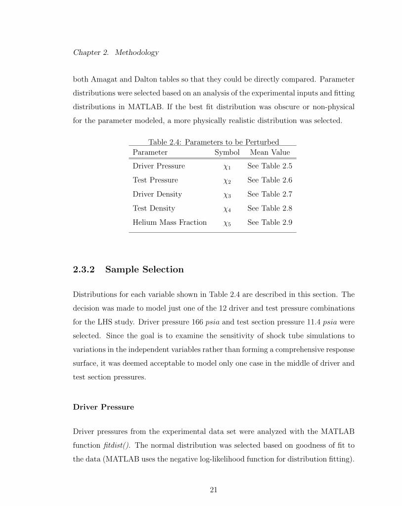
both Amagat and Dalton tables so that they could be directly compared. Parameter
distributions were selected based on an analysis of the experimental inputs and fitting
distributions in MATLAB. If the best fit distribution was obscure or non-physical
for the parameter modeled, a more physically realistic distribution was selected.
Table 2.4: Parameters to be Perturbed
Parameter Symbol Mean Value
Driver Pressure χ1 See Table 2.5
Test Pressure χ2 See Table 2.6
Driver Density χ3 See Table 2.7
Test Density χ4 See Table 2.8
Helium Mass Fraction χ5 See Table 2.9
2.3.2 Sample Selection
Distributions for each variable shown in Table 2.4 are described in this section. The
decision was made to model just one of the 12 driver and test pressure combinations
for the LHS study. Driver pressure 166 psia and test section pressure 11.4 psia were
selected. Since the goal is to examine the sensitivity of shock tube simulations to
variations in the independent variables rather than forming a comprehensive response
surface, it was deemed acceptable to model only one case in the middle of driver and
test section pressures.
Driver Pressure
Driver pressures from the experimental data set were analyzed with the MATLAB
function fitdist(). The normal distribution was selected based on goodness of fit to
the data (MATLAB uses the negative log-likelihood function for distribution fitting).
21

Chapter 2. Methodology
Mean driver pressures and standard deviations were used as inputs into DAKOTA to
define the parameter distributions. Table 2.5 details three different nominal driver
pressures and the corresponding normal distribution parameters. The decision was
made to bound the normal distributions at ±3.08σ for each case, including ±3.08σ
corresponds to 99.8% of expected values [27]. The formula for the normal distribution
is
f(x) =1
σ√
2πexp
[−(x− µ)2
2σ2
], (2.13)
where µ is the mean and σ is the standard deviation.
Table 2.5: χ1 (Driver Pressure) Normal Distribution Fits
Case µ[dynecm2
]σ[dynecm2
]- Bound
[dynecm2
]+ Bound
[dynecm2
]146 psia 10.06977×10⁶ 5.537×10³ 10.05272×10⁶ 10.08682×10⁶
166 psia 11.44710×10⁶ 13.283×10³ 11.40619×10⁶ 11.48801×10⁶
186 psia 12.82305×10⁶ 6.013×10³ 12.80453×10⁶ 12.84158×10⁶
Test Section Pressure
Because experimental test section pressures varied little, σ ≈ O(10−16), a triangular
distribution
f(x) =
0 b < x or x < a
2(x−a)(b−a)(c−a) a ≤ x < c
2b−a x = c
2(b−x)(b−a)(b−c) c < x ≤ b
(2.14)
was used. The triangular distribution is defined with minimum and maximum values,
a and b, respectively, and mode, c (a ≤ c ≤ b). Test pressure distribution param-
eters are shown in Table 2.6. The upper and lower bounds, b and a, respectively,
22

Chapter 2. Methodology
correspond to a variation of ±0.2 psia1, about the same as the worst case variation
seen in the driver section.
Table 2.6: χ2 (Test Pressure) Triangular Distribution Fits
Case a[dynecm2
]b[dynecm2
]c[dynecm2
]1.14 psia 6.4811×10⁴ 9.2390×10⁴ 7.8600×10⁴
5.70 psia 37.9212×10⁴ 40.6791×10⁴ 39.3001×10⁴
11.4 psia 77.2213×10⁴ 79.9792×10⁴ 78.6002×10⁴
17.1 psia 116.5214×10⁴ 119.2793×10⁴ 117.9003×10⁴
Driver and Test Section Densities
CTH requires the independent thermodynamic values of an input deck for our prob-
lem to be pressure and density. In the experiment, pressure and temperature were
measured directly. Thus the SESAME tables were interrogated to determine the
range of the densities based on the range in the temperature (T ∈ [293.305, 297.155]
K) at the pressures listed in Table 2.2 for the test section. The driver densities
shown in Table 2.7 are fitted with a triangular distribution as described in Equation
2.14. Pure helium gas was used for the experiments as the driver section gas. Since
pure helium behaves as an ideal gas over the range of pressures and temperatures
simulated the densities could be computed directly from Equation 2.1. Test section
densities were also modeled with the triangular distribution and the distribution
parameters are shown in Table 2.8.
Helium Mass Fraction
Helium mass fraction was varied to simulate uncertainty in the experimental mixing.
Bounded normal distribution parameters used to simulate this variance are shown
1A pressure of 1 psia ≈ 68, 947.55 dynecm2
23

Chapter 2. Methodology
Table 2.7: χ3 (Drive Densities) Triangular Distribution Fits
Case a[
gcm3
]b[
gcm3
]c[
gcm3
]146 psia 1.6304×10⁻³ 1.6518×10⁻³ 1.6410×10⁻³
166 psia 1.8537×10⁻³ 1.8780×10⁻³ 1.8658×10⁻³
186 psia 2.0770×10⁻³ 2.1043×10⁻³ 2.0906×10⁻³
Table 2.8: χ4 (Test Density) Triangular Distribution Fits
Case a[
gcm3
]b[
gcm3
]c[
gcm3
]1.14 psia 3.2887×10⁻⁴ 3.3468×10⁻⁴ 3.3176×10⁻⁴
5.70 psia 11.6073×10⁻⁴ 14.8748×10⁻⁴ 13.2230×10⁻⁴
11.4 psia 23.1943×10⁻⁴ 27.9275×10⁻⁴ 25.5376×10⁻⁴
17.1 psia 34.7671×10⁻⁴ 39.9328×10⁻⁴ 37.3208×10⁻⁴
in Table 2.9.
Table 2.9: χ5 (Helium Mass Fraction) Normal Distribution Fits
µ σ - Bound + Bound
0.0267 0.0033 0.0165 0.0369
The upper and lower bounds were selected based on estimates of variation in the He
mole fraction
xHe =nHe
nHe + nSF6
, (2.15)
where ni is the number of moles of component i. Utilizing the relation m = nM
allows Equation 2.15 to be transformed into a form dependent on mass fraction wHe.
xHe =1
1 + MHe
MSF6
(w−1He + 1
) . (2.16)
For wHe = 0.0267 ± 0.01 the mole fraction takes on the values xHe ≈ [0.38, 0.58],
which could have a significant affect on the shock characteristics.
24

Chapter 3
Results
All 12 experimental nominal pressure combinations were simulated in CTH. During
the course of the analysis it became convenient to express the shock speed and shock
temperature as functions of the dimensionless pressure ratio
φ =PDriver
PTest
. (3.1)
Nominal pressures are used to determine the value of φ, which had the convenient
effect of allowing shock speed and shock temperature results to each be displayed
on single curves. Plotting the shock speeds and shock temperatures a function of φ
allowed graphical analysis of the differences between the Amagat and Dalton formu-
lations. Pressure ratios used are listed in Table 3.1.
Shock speed, temperature, and pressure are not simple functions of pressure ratio.
Rather, the thermodynamic characteristics of what is driving the shock as well as
the gas mixture into which the shock is traveling determine measured shock speeds,
pressures, and temperatures. This became clearly evident after it was discovered
that the experimental work had used pure helium as driver gas while preliminary
numerical simulations assumed a driver gas of 50:50 molar mixture of helium and
SF6, resulting in wildly different shock characteristics. Furthermore, shock pressure
25

Chapter 3. Results
Table 3.1: Pressure Ratios
φ PDriver [psia] PTest [psia]
128.1 146 1.1425.6 146 5.7012.8 146 11.48.5 146 17.1
145.6 166 1.1429.1 166 5.7014.6 166 11.49.7 166 17.1
163.2 186 1.1432.6 186 5.7016.3 186 11.410.9 186 17.1
is not well described as a function of a pressure ratio, but rather as a surface that is
described by both driver and test section pressures.
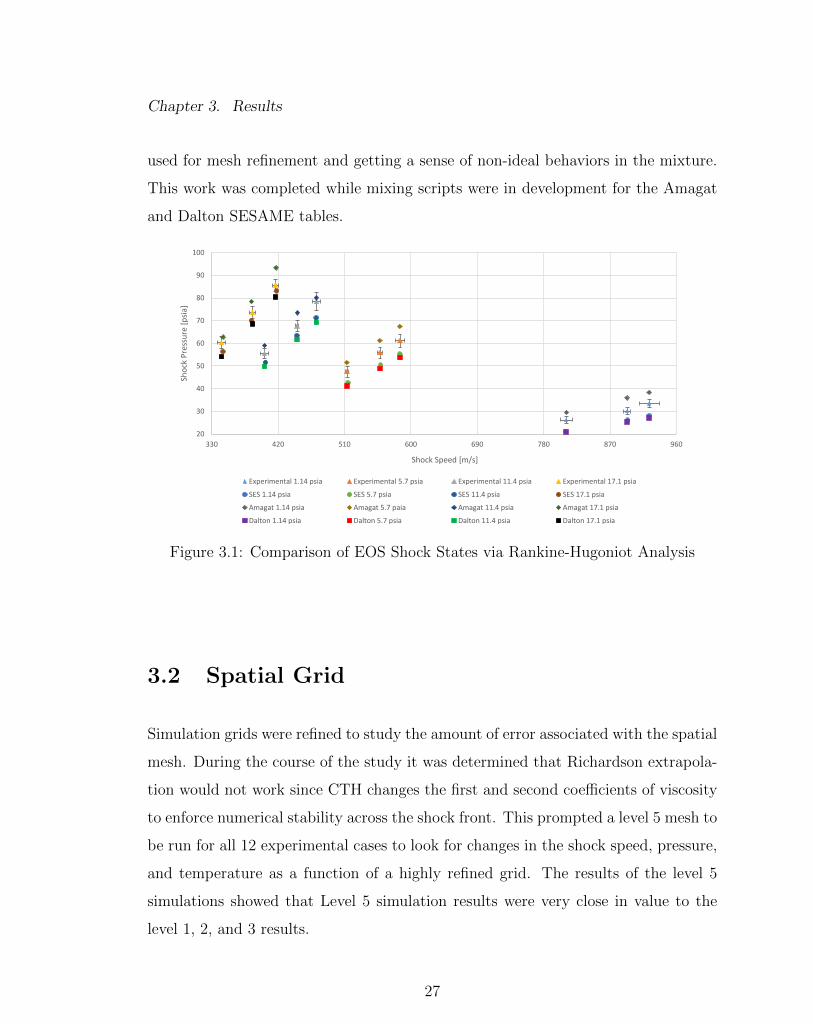
3.1 EOS Verification
EOS surfaces were analyzed prior to running simulations in CTH to ensure that they
passed through the thermodynamic states of interest. The BCAT subroutine allows
for Rankine-Hugoniot analysis of an EOS, which permitted a direct comparison of
shock speed and shock pressure from the experiment. Rankine-Hugoniot results are
shown in Figure 3.1.
In general, Amagat formulation data (diamond points) most closely matches experi-
mental values, which are shown with error bars. SESAME tables computed directly
from TIGER mixing and Dalton mixing most closely match one another (circle and
square points, respectively). All data points are relatively close to the experimental
values demonstrating the ability of every SESAME EOS used to approximately pass
through the shock states measured in the experiment. TIGER EOS files were only
26
Chapter 3. Results
used for mesh refinement and getting a sense of non-ideal behaviors in the mixture.
This work was completed while mixing scripts were in development for the Amagat
and Dalton SESAME tables.
Case Speed [m/s] Speed dev. Exp. P. [psi] St. Dev. [psi] Speed [m/s] SES P. [Gpa] SES P. [psi] SES Error Amagat [m/s] Amagat P. [Gpa]
146_1 810.72 7.791 26.2 1.41 810 1.45E-04 21.03 10.95% 810.98 2.03E-04
146_5 513.46 2.353 47.5 2.49 514.71 2.94E-04 42.59 5.45% 513.23 3.55E-04
146_11 401.62 5.292 55.5 2.08 402.9 3.56E-04 51.61 3.63% 401.82 4.07E-04
146_17 343.21 5.876 60.3 2.65 345.3 3.88E-04 56.32 3.41% 345.4 4.33E-04
166_1 893.15 4.366 30.1 1.69 893.84 1.80E-04 26.09 7.13% 893.1 2.47E-04
166_5 558.12 2.974 55.8 2.53 558.97 3.47E-04 50.36 5.13% 557.9 4.22E-04
166_11 445.68 2.371 67.7 2.47 445.6 4.37E-04 63.38 3.30% 446.2 5.06E-04
166_17 385.34 4.483 73.6 2.54 383.8 4.82E-04 69.97 2.53% 383.91 5.40E-04
186_1 923.1 13.692 33.4 1.64 923.1 1.93E-04 28.02 8.75% 923.1 2.64E-04
186_5 585.23 6.145 61.1 2.99 585.1 3.81E-04 55.25 5.03% 585.2 4.65E-04
186_11 471.81 5.826 78.4 3.83 471.7 4.91E-04 71.19 4.82% 471.8 5.52E-04
186_17 416.43 4.178 85.7 2.64 417.99 5.73E-04 83.13 1.52% 417.3 6.43E-04
20
30
40
50
60
70
80
90
100
330 420 510 600 690 780 870 960
Sho
ck P
ress
ure
[p
sia]
Shock Speed [m/s]
Shock Pressure vs Shock Speed
Experimental 1.14 psia Experimental 5.7 psia Experimental 11.4 psia Experimental 17.1 psia
SES 1.14 psia SES 5.7 psia SES 11.4 psia SES 17.1 psia
Amagat 1.14 psia Amagat 5.7 paia Amagat 11.4 psia Amagat 17.1 psia
Dalton 1.14 psia Dalton 5.7 psia Dalton 11.4 psia Dalton 17.1 psia
Figure 3.1: Comparison of EOS Shock States via Rankine-Hugoniot Analysis
3.2 Spatial Grid
Simulation grids were refined to study the amount of error associated with the spatial
mesh. During the course of the study it was determined that Richardson extrapola-
tion would not work since CTH changes the first and second coefficients of viscosity
to enforce numerical stability across the shock front. This prompted a level 5 mesh to
be run for all 12 experimental cases to look for changes in the shock speed, pressure,
and temperature as a function of a highly refined grid. The results of the level 5
simulations showed that Level 5 simulation results were very close in value to the
level 1, 2, and 3 results.
27

Chapter 3. Results
Simulated shock speeds were not monotonic with mesh size, indicating that it is
most affected by changes to viscosity coefficients and so, extrapolations were not
very helpful. Instead the value of the shock speed was compared between the mesh
levels 2 and 3 described in Table 2.3. Numerical error is presented in Table 3.2 and
is the absolute percent error relative to f3.
Table 3.2: Shock Speed Refinement Error
φ f2 [m/s] f3 [m/s] |ε23|128.1 932.8933 932.2836 0.065%25.6 602.2975 601.7222 0.096%12.8 483.6105 483.3302 0.058%8.5 422.0700 421.8304 0.057%
145.6 961.9362 961.6693 0.028%29.1 626.1377 625.7848 0.056%14.6 504.2622 504.0943 0.033%9.7 441.0974 440.8154 0.064%
163.2 988.2076 987.5557 0.066%32.6 647.7944 647.2558 0.083%16.3 523.2217 523.0088 0.041%10.9 458.4630 458.1232 0.074%
Shock pressure and temperature behaved more like one would expect with spatial
grid refinement. The simulated values were generally monotonic with mesh refine-
ment and showed something like O(h) convergence with some notable exceptions.
However, due to the nature of the changing coefficients of viscosity extrapolation
values do not tell the whole story. Tables 3.3 and 3.4 show the absolute percent error
relative to levels 2 and 3. There is very little difference between the levels indicating
that additional spatial refinement is not needed. A level 5 mesh produced shock
pressures and temperatures very similar to the level 1, 2, and 3 mesh results.
28

Chapter 3. Results
Table 3.3: Shock Pressure Refinement Error
φ f2 [psia] f3 [psia] |ε23|128.1 28.6965 28.6911 0.019%25.6 58.6622 58.6610 0.002%12.8 74.6633 74.7866 0.165%8.5 83.7313 83.8758 0.172%
145.6 30.5326 30.5253 0.024%29.1 63.4755 63.4749 0.001%14.6 81.6538 81.6727 0.023%9.7 91.8446 91.9482 0.113%
163.2 32.2185 32.2115 0.022%32.6 67.9922 67.9923 0.000%16.3 88.0465 88.0270 0.022%10.9 99.6717 99.8062 0.135%
Table 3.4: Shock Temperature Refinement Error
φ f2 [K] f3 [K] |ε23|128.1 717.703 716.580 0.157%25.6 486.813 484.837 0.408%12.8 420.023 419.908 0.027%8.5 388.784 388.821 0.010%
145.6 741.819 740.513 0.176%29.1 500.991 498.917 0.416%14.6 431.265 430.613 0.151%9.7 397.877 397.828 0.012%
163.2 763.953 762.390 0.205%32.6 514.209 512.411 0.351%16.3 441.636 440.482 0.262%10.9 406.540 406.503 0.009%
3.3 Shock Tube Simulations
Shock tube simulation outputs were analyzed via MATLAB scripts to determine
shock quantities of interest (QoI), namely shock speed, pressure, and temperature.
29

Chapter 3. Results
Analysis was performed via MATLAB scripts which looked for change in velocity
at the tracer for shock speed and maximum temporal derivatives for post-shock
temperature and pressure. More information on MATLAB scripts is presented in
Appendix C.
3.3.1 Shock Speed, Us
We found by inspection of the plots and by curves of best fit, that Amagat and
Dalton results converge as the pressure ratio approaches unity. This makes some
intuitive sense as there is not as much disparity in pressure energy between the drive
and test gases. Thus, there is less ability of the drive section to push on the test
section, resulting in weaker shocks that propagate more slowly. In addition, both
the drive and test sections were initialized in the simulation at room temperature
(295 K). Thus any increase in energy must come solely from the pressure imbalance.
This is most evident in the trends shown by shock speed as a function of pressure
ratio shown in Figure 3.2. As is shown, the higher the pressure ratio, the faster
the shock speed. Both Amagat and Dalton simulation data was fit using a curve of
best fit of the form Us(φ) = a ln(φ) + b. Best fit coefficients were determined using
linear least squares and the value of the coefficient of determination was computed,
resulting in a value of approximately 0.95. Grouping in clusters of three is due to
distinct groupings of the pressure ratios as is shown in Table 3.1. One will notice
that the data points do not fall exactly onto the logarithmic curves. This is due to
the fact that some information about the shock speed is contained in the test section
pressure and density. To fully describe the shock speed, one needs more than one
dimension.
The curves nicely capture the Amagat and Dalton trends and show that Dalton
tends to overestimate the experiment when using the same pressures and initial
temperatures. For the purposes of investigating the differences between the mixing
30

Chapter 3. Results
0 20 40 60 80 100 120 140 160 180300
400
500
600
700
800
900
1000
1100
AmagatDaltonAmagat FitDalton FitExperimental
Figure 3.2: Shock Speed Versus Pressure Ratio
models, we find that using pressure ratio is a good way to compare the results.
However, we do not claim that a fit based on pressure ratio alone is necessarily a good
predictor of shock tube results. As one achieves higher pressure ratios in the shock
tube, the disparity between Amagat and Dalton models becomes more pronounced
indicating that Amagat and Dalton predictions may diverge further with even higher
pressure ratios. Error between simulation and experimental results is shown in Table
3.5. Error was calculated using a normalized difference
ε =xexperimental − xsimulated
xexperimental· 100%, (3.2)
where xexperimental is the measured value and xsimulated is the simulated value. As is
shown in Figure 3.2 and Table 3.5, the 2D simulation tends to have lower error at
higher pressure ratios. At some of the lower pressure ratios the error is unacceptably
high, however, this may be overcome by running the simulations in 3D instead of 2D.
Overall, Amagat simulation values match experiment better than Dalton simulation
values. Error is primarily reduced by modeling the transition from round to square
31
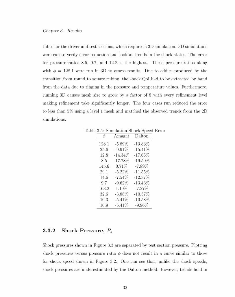
Chapter 3. Results
tubes for the driver and test sections, which requires a 3D simulation. 3D simulations
were run to verify error reduction and look at trends in the shock states. The error
for pressure ratios 8.5, 9.7, and 12.8 is the highest. These pressure ratios along
with φ = 128.1 were run in 3D to assess results. Due to eddies produced by the
transition from round to square tubing, the shock QoI had to be extracted by hand
from the data due to ringing in the pressure and temperature values. Furthermore,
running 3D causes mesh size to grow by a factor of 8 with every refinement level
making refinement take significantly longer. The four cases run reduced the error
to less than 5% using a level 1 mesh and matched the observed trends from the 2D
simulations.
Table 3.5: Simulation Shock Speed Errorφ Amagat Dalton
128.1 -5.89% -13.83%25.6 -9.91% -15.41%12.8 -14.34% -17.65%8.5 -17.78% -19.50%
145.6 0.71% -7.89%29.1 -5.22% -11.55%14.6 -7.54% -12.37%9.7 -9.62% -13.43%
163.2 1.19% -7.27%32.6 -3.88% -10.37%16.3 -5.41% -10.58%10.9 -5.41% -9.96%
3.3.2 Shock Pressure, Ps
Shock pressures shown in Figure 3.3 are separated by test section pressure. Plotting
shock pressures versus pressure ratio φ does not result in a curve similar to those
for shock speed shown in Figure 3.2. One can see that, unlike the shock speeds,
shock pressures are underestimated by the Dalton method. However, trends hold in
32

Chapter 3. Results
that the Dalton and Amagat results do not cross and the disparity in the predictions
grows with increasing pressure ratio. Indicating the Amagat and Dalton EOS sur-
faces predict different thermodynamic states across the range of pressure ratios with
increasing disparity at more extreme pressure ratios.
120 130 140 150 160 17020
25
30
35
40
24 26 28 30 32 3440
45
50
55
60
65
12 13 14 15 16 1750
60
70
80
90
8.5 9 9.5 10 10.5 1150
60
70
80
90
AmagatDaltonExperimental
Figure 3.3: Shock Pressure Into Various Test Section Pressures
Experimental values cross over the two models at low values of φ. This may be be-
cause of error inherent in the 2D simulation or model form error inherent to Amagat
and Dalton mixtures. In general, Amagat tends to be the better predictor of shock
pressure. However, one may note that the difference between Amagat and Dalton
predictions is nearly constant with pressure ratio for each test section pressure. Sim-
ulation error with respect to experiment is tabulated in Table 3.6 shows that the
Amagat method is the better predictor of shock pressure with the notable excep-
tions of φ = 8.5 and φ = 12.8. Unlike the shock speed, error improves with lower
33

Chapter 3. Results
pressure ratios. Most of the errors are < 10% indicating that Amagat is relatively
accurate. However, at certain values of φ the error is as high as 15%. Running more
computationally expensive 3D models would reduce this error as discussed previously
if very accurate models of the shock tube were desired.
Table 3.6: Simulation Shock Pressure Error
φ Amagat Dalton
128.1 4.57% 23.34%25.6 0.58% 8.72%12.8 -6.02% -0.83%8.5 -9.45% -5.21%
145.6 11.26% 33.20%29.1 8.30% 18.24%14.6 5.15% 11.11%9.7 1.84% 5.91%
163.2 15.39% 40.19%32.6 10.08% 20.89%16.3 11.63% 19.52%10.9 8.67% 14.03%
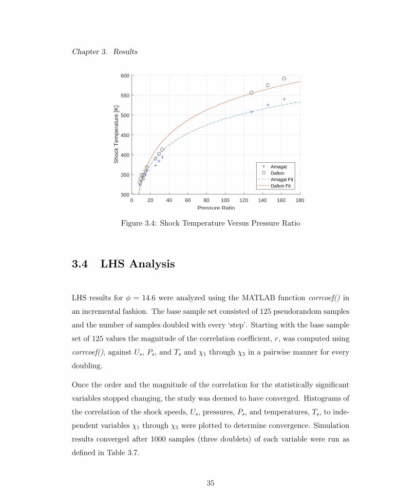
3.3.3 Shock Temperature, Ts
Shock temperatures were not measured in the initial experimental work. Simulated
temperatures are shown in Figure 3.4 plotted versus pressure ratio. The dependence
on the test section pressures becomes apparent in Figure 3.4 as the groups of data
points have a more pronounced defect from the curves of fit. As with shock speed,
shock temperatures were fit with curves of the form Ts(φ) = a ln(φ)+b. Calculation of
the coefficient of determination resulted in a value of approximately 0.91. The trend
continues to hold that Dalton and Amagat are clearly different without crossing each
other over the range of pressure ratios studied.
34
Chapter 3. Results
0 20 40 60 80 100 120 140 160 180
Pressure Ratio
300
350
400
450
500
550
600
Sho
ck T
empe
ratu
re [K
]
AmagatDaltonAmagat FitDalton Fit
Figure 3.4: Shock Temperature Versus Pressure Ratio
3.4 LHS Analysis
LHS results for φ = 14.6 were analyzed using the MATLAB function corrcoef() in
an incremental fashion. The base sample set consisted of 125 pseudorandom samples
and the number of samples doubled with every ‘step’. Starting with the base sample
set of 125 values the magnitude of the correlation coefficient, r, was computed using
corrcoef(), against Us, Ps, and Ts and χ1 through χ5 in a pairwise manner for every
doubling.
Once the order and the magnitude of the correlation for the statistically significant
variables stopped changing, the study was deemed to have converged. Histograms of
the correlation of the shock speeds, Us, pressures, Ps, and temperatures, Ts, to inde-
pendent variables χ1 through χ5 were plotted to determine convergence. Simulation
results converged after 1000 samples (three doublets) of each variable were run as
defined in Table 3.7.
35

Chapter 3. Results
Table 3.7: Parameters Perturbed in LHS Study
Parameter Symbol Mean Value
Driver Pressure χ1 11.44710×10⁶ dyne/cm2
Test Pressure χ2 78.6002×10⁴ dyne/cm2
Driver Density χ3 1.8658×10⁻³ g/cm3
Test Density χ4 25.5376×10⁻⁴ g/cm3
Helium Mass Fraction χ5 0.0267
x4 x5 x1 x3 x20
0.2
0.4
0.6
0.8
1
x4 x5 x1 x3 x20
0.2
0.4
0.6
0.8
1
x4 x5 x1 x2 x30
0.2
0.4
0.6
0.8
1
x4 x5 x1 x2 x30
0.2
0.4
0.6
0.8
1
x5 x4 x2 x1 x30
0.2
0.4
0.6
0.8
1
x5 x4 x2 x1 x30
0.2
0.4
0.6
0.8
1
Figure 3.5: LHS QoI Results Run Against 1000 Samples
36

Chapter 3. Results
Figure 3.5 shows the final results of the LHS study summarized with Amagat and
Dalton QoI (Quantities of Interest) in the left and right columns, respectively. As
is shown both the Amagat and Dalton models are most sensitive to χ4, test section
density, and χ5, helium mass fraction. However, which variable has the strongest
relationship depends on the QoI. The sensitivity of the two models is quite similar
in magnitude and ordering of variables, χi, based on the correlation strength. Only
shock pressure shows a significant difference in sensitivity between the Amagat and
Dalton models in the second-most influential paramters χ5, helium mass fraction.
Amagat Dalton460
480
500
520
Amagat Dalton80
82
84
86
Amagat Dalton350
400
450
500
550
Figure 3.6: Comparison of Amagat and Dalton LHS Results
Statistics of the LHS results of Amagat and Dalton mixtures are shown in Figure 3.6.
The minimum, mean, and maximum values are superimposed on a plot of standard
37

Chapter 3. Results
deviation (±1σ) of each mixing model for each QoI. Unlike the results in Section 3.3
compared to experimental values, the Amagat model predicts faster shock speeds,
higher shock pressures, and higher shock temperatures overall than the Dalton model
does for the same initial pressures and densities. Simulations for the LHS study were
run for the same initial pressures and densities which resulted in different initial
temperatures of the test section mixture for the Amagat and Dalton models. Recall
that CTH requires the initial pressure and density or temperature and density to be
specified. In simulations compared to experimental results in Section 3.3, density
was set from experimental initial pressure and temperature. This led to different
initial density values depending on whether an Amagat or Dalton EOS was used.
Differences between shock speed and pressure distributions are not large, with shifts
of 5 m/s and 1 psia, respectively. However, a difference of roughly 50 K is seen in
the shock temperature predictions, which is significant for the given shock regime.
Results from CTH simulations show that for the same input values, Amagat and
Dalton EOS mixtures will predict different shock characteristics. Another way to
think about the problem is to ask, ‘if simulation initial conditions were perturbed
in the Amagat and Dalton simulations, how much would the models agree?’ This is
shown to some degree in Figure 3.6, but does not yield a quantitative result. Using
the MATLAB function fitdist(), we fit the LHS study QoI with probability density
functions (generalized extreme value) over their respective range of values. We then
calculated the coefficient of overlap, Covl, between the two distributions and plotted
the results [30, 31].
3.4.1 Shock Speed, Us
Figure 3.7 shows that there exists strong agreement between the Amagat and Dal-
ton EOS when it comes to predicting the shock speed. The overlap between the two
distributions comprises 80.58% of the simulated values based on the value of Covl.
38

Chapter 3. Results
One way of thinking about this result is that that the distance between the Amagat
and Dalton shock speed distributions is not large.
475 480 485 490 495 500 505 510 515 5200
0.01
0.02
0.03
0.04
0.05
0.06
Amagat SpeedsDalton Speeds
Figure 3.7: Overlap in Shock Speed Distributions, Covl = 0.8058
3.4.2 Shock Pressure, Ps
Similarly, shock pressures were analyzed are shown in Figure 3.8. The results show
that the pressures also have strong agreement, as the overlap constitutes 75.27% of
the simulated values. While slightly less than shock speed overlap, the agreement
between the two distributions is still significant.
39

Chapter 3. Results
80.5 81 81.5 82 82.5 83 83.5 84 84.5 850
0.1
0.2
0.3
0.4
0.5
0.6
Amagat PressuresDalton Pressures
Figure 3.8: Overlap in Shock Pressure Distributions, Covl = 0.7527
3.4.3 Shock Temperature, Ts
The shock temperatures showed the most disparity between the two models as the
overlap only accounted for 29.02% of the simulated values. Figure 3.9 shows the two
temperature distributions and the region of overlap. This is the strongest difference
between the two models.
In summary, we have shown that the Amagat mixing model provides the best agree-
ment with the experimental results and that those results are distinctly different
40

Chapter 3. Results
from the Dalton model. Furthermore, we have shown that for the same initial condi-
tions the Dalton model will tend to overpredict the experimental values as opposed
to LHS values where it underestimates shock QoI. We believe that the reason for
Dalton overestimation had to do with the way CTH requires initial conditions be set
as pressure and density versus pressure and temperature. Thus, when the shocktube
was simulated, different densities would be provided depending on the EOS so that
the simulations started off at the same temperature. Finally, when comparing per-
turbations of the initial conditions we show that the strongest disparity between the
simulated results occurs in the prediction of shock temperature.
340 360 380 400 420 440 460 480 500 5200
0.005
0.01
0.015
0.02
0.025
Amagat TemperaturesDalton Temperatures
Figure 3.9: Overlap in Shock Temperature Distributions, Covl = 0.2902
41

Chapter 4
Conclusions & Future Work
4.1 Conclusions
Based on the modeling of the shock tube as shown in Figures 3.2, 3.3, and 3.4 we
conclude that there is a difference between the Amagat and Dalton EOS models. The
greatest differences occur when looking at the shock speed and shock temperature.
This can be explained, as was noted in Chapter 3, by the fact that the densities were
used to set the temperature of the simulation. By setting the same pressures and
different densities to achieve the same temperatures, we were acknowledging that the
EOS surfaces were predicting different thermodynamic states for the mixture. This
affected the outcomes as has been shown. LHS results show the strongest agreement
between Amagat and Dalton models in the shock speed and the worst agreement in
the shock temperatures. In addition, the LHS results showed that the shock pressure
has the most complicated relationship to the input parameters perturbed. Shock
speed and shock temperature were dominated by variables χ4 and χ5. Shock pressure,
while still predominately dependent on χ4 and χ5, has a stronger relationship with
χ1, χ2, and χ3 than either shock speed or shock temperature. This can be seen in
42

Chapter 4. Conclusions & Future Work
the magnitudes of the correlation coefficients in Figure 3.5. Furthermore the LHS
analysis showed that while the Amagat and Dalton EOS models were sensitive to
essentially the same parameters, it also showed that both predict different shock
speeds, pressures, and temperatures. The only way to get agreement between the
shock characteristics is to allow the initial conditions to vary. Experience running
the simulations has shown that the forcing agreement may require nonsensical initial
conditions in the simulation, which defeats the purpose of modeling. As was shown in
Figures 3.7, 3.8, and 3.9 the models only agree well on 2 out of the 3 characteristics.
This implies that the models cannot simultaneously agree on both pressure and
temperature of the mixture. If agreement is forced in the temperatures, the pressure
will fail to agree and vice versa. When modeling inert gases undergoing shocks, we
see that Amagat and Dalton mixing do not give the same results. In general the
Amagat model results are in significantly better agreement with the experimental
data for shock speed and shock pressure. Forthcoming experimental results for shock
temperature will be important in assessing whether one model is clearly superior in
predicting results for mixed gases undergoing shock.
4.2 Future Work
In the course of performing research one finds out how very little they are able to push
the boundary of knowledge, even when expending considerable amounts of effort and
resources. There is usually more work to do and, in the very least, refinements to be
made. This work could be improved and expanded in a number of ways:
• Run more LHS studies to develop mixing response surfaces
• Study other gaseous mixtures
• Study reacting gases or ionizing gases (TIGER can model ionized gases)
43

Chapter 4. Conclusions & Future Work
• Look at mixtures with more than two constituents
• Consider some form of phase change
One advantage of LHS studies, is that they provide insight into which parameters
drive variation in the model. One way in which this work could be used would be to
explore how restricting the variation of the LHS input distributions affect results.
The preceding list only begins to scratch the surface possible improvements or ad-
ditions. This research showed that a difference exists between Amagat and Dalton
mixtures but further development is needed to understand how the differences af-
fect predictions. In addition, the LHS analysis showed that test section density and
mixture mass fraction had strong influence over the shock speed, pressure, and tem-
perature. This could inform new experiments by better controlling either variable
and then adding in known variations. One example would be heating or cooling
the test section to achieve different shock speeds. Addressing model form error by
parametrizing χ4 and χ5 would mitigate, or at least provide control over, model
sensitivity in the Amagat and Dalton representations. This could take many forms
and may be an avenue for research that would provide insight into mixture physics.
Finally, extending this work to other gases may help formalize good modeling and
simulation practices in the realm of gas dynamics.
44

Appendices
45

Appendix A
Sample CTH Input
Below is a sample of a CTH input deck used in the simulations performed in this
research.
**********************************************************************
*eor* cthin
*
**********************************************************************
Shocktube with He and SF6 Dalton SESAME EOS Refinement Level 3
* Mesh Level 1
* Driver pressure: 1.1458e+07
* Driver density: 1.8596e-03
* Test pressure: 7.9047e+05
* Test density: 2.4731e-03
control
mmp
tstop = 8.5e-3
endc
46
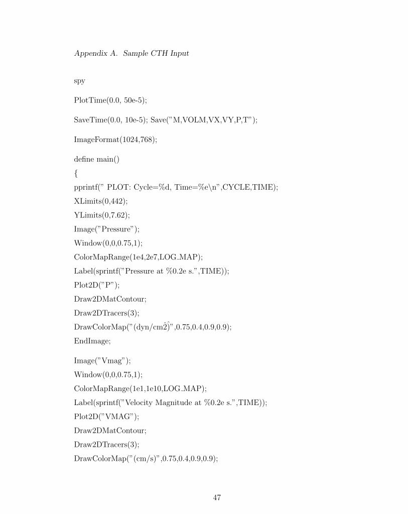
Appendix A. Sample CTH Input
spy
PlotTime(0.0, 50e-5);
SaveTime(0.0, 10e-5); Save(”M,VOLM,VX,VY,P,T”);
ImageFormat(1024,768);
define main()
{
pprintf(” PLOT: Cycle=%d, Time=%e\n”,CYCLE,TIME);
XLimits(0,442);
YLimits(0,7.62);
Image(”Pressure”);
Window(0,0,0.75,1);
ColorMapRange(1e4,2e7,LOG MAP);
Label(sprintf(”Pressure at %0.2e s.”,TIME));
Plot2D(”P”);
Draw2DMatContour;
Draw2DTracers(3);
DrawColorMap(”(dyn/cm2)”,0.75,0.4,0.9,0.9);
EndImage;
Image(”Vmag”);
Window(0,0,0.75,1);
ColorMapRange(1e1,1e10,LOG MAP);
Label(sprintf(”Velocity Magnitude at %0.2e s.”,TIME));
Plot2D(”VMAG”);
Draw2DMatContour;
Draw2DTracers(3);
DrawColorMap(”(cm/s)”,0.75,0.4,0.9,0.9);
47

Appendix A. Sample CTH Input
EndImage;
Image(”Temperature”);
Window(0,0,0.75,1);
ColorMapRange(0,.07);
Label(sprintf(”Temperature at %0.2e s.”,TIME));
Plot2D(”T”);
Draw2DMatContour;
Draw2DTracers(3);
DrawColorMap(”(eV)”,0.75,0.4,0.9,0.9);
EndImage;
}
HisTime(0,1e-6);
SaveTracer(ALL);
SaveHis(”GLOBAL,POSITION,P,T,DENS,VX,VY”);
define spyhis main()
{
HisLoad(1,”hscth”);
Label(”Pressure at Tracer 1”);
TPlot(”P.1”,1,AUTOSCALE);
Label(”Pressure at Tracers 2-6”);
TPlot(”P.2”,1,AUTOSCALE);
TDraw(”P.3”,1);
TDraw(”P.4”,1);
TDraw(”P.5”,1);
TDraw(”P.6”,1);
}
endspy
48

Appendix A. Sample CTH Input
mesh
*
block 1 geom=2dr type=e
*
x0 0.
x1 n=408 ratio=1 w=442
endx
*
y0 0.
y2 n=8 ratio=1 w=7.62
endy
endb
*
endm
convct
interface=smyra
endc
**********************************************************************
*
* equation of state inputs
*
eos SES=500000
mat1 SES USER EOS=9997 FEOS=’b9997’
mat2 IDGAS USER cv=3.61501e11 GM1=0.667
endeos
tracer
add 100,3.81 fixed=xy
add 161.985,3.81 fixed=xy
49

Appendix A. Sample CTH Input
add 233.105,3.81 fixed=xy
add 330.895,3.81 fixed=xy
add 402.015,3.81 fixed=xy
endtracer
* material insertion inputs
diatom
package ’hipressure’
mat 2
pressure 1.14577e+07
density 1.85956e-03
insert box
p1 = 0,0
p2 = 122,7.62
endinsert
endpackage
package ’lopressure’
mat 1
pressure 7.90466e+05
density 2.47313e-03
insert box
p1 = 122,0
p2 = 442,7.62
endi
endp
enddiatom
edit
shortt
tim = 0., dt = 1e-5
50
Appendix A. Sample CTH Input
ends
*
longt
tim = 0., dt = 1.0
endl
restt
tim = 0.
dtf = 5e-5
endr
*
ende
boundary
bhydro
bxbot = 0 , bxtop = 0
bybot = 0 , bytop = 0
endhydro
endb
mindt
time = 0. dt = 1.e-9
endn
51

Appendix B
Mesh Convergence
B.1 SESAME Grid Convergence
SESAME table refinement studied EOS sensitivity to grid spacing in the T, v, P and
T, v, e surfaces. In this instance when we say ‘grid’ we are referring to the spacing
of the thermodynamic points and not the spatial mesh. As described in Table 2.1,
we used refinement levels to study the relative errors of the shock speeds when using
different resolutions of SESAME tables. The configurations run are shown in Table
B.1. Absolute relative error was computed using
δ =|x1 − x2|
0.5(x1 + x2), (B.1)
where x1 and x2 are any two variables with the same units. Convergence was as-
sumed if δ ≤ 1× 10⁻³. The shock speeds were compared between levels 1 to 2, 2 to
3, and 1 to 3. Figure B.1 shows the relative error between and demonstrates that in
all but one case the simulation could be considered converged at level 1 refinement.
Each ring of Figure B.1 corresponds to an error magnitude relative to the previous
SESAME refinement level. Radial lines in Figure B.1 correspond to a combination
of driver and test section pressures listed in Table B.1. Recall that a level 1 refine-
52

Appendix B. Mesh Convergence
ment corresponded to a ∆T = 24K and ∆v = 50 cm3
g. Each subsequent refinement
halved the property step size. All simulations in this thesis were run with a level 3
refinement.
Table 146_1 146_5 146_11 146_17 166_1 166_5 166_11 166_17
1 to 3 1.04E-04 1.89E-03 4.27E-04 2.17E-04 1.28E-04 2.12E-05 2.19E-04 1.32E-04
1 to 2 3.77E-04 1.29E-03 3.01E-04 2.72E-05 7.98E-05 3.18E-04 2.43E-05 2.65E-05
2 to 3 2.73E-04 6.08E-04 1.26E-04 2.45E-04 4.79E-05 3.39E-04 2.43E-04 1.59E-04
0.00E+00
4.00E-04
8.00E-04
1.20E-03
1.60E-03
2.00E-03146_1
146_5
146_11
146_17
166_1
166_5
166_11
166_17
186_1
186_5
186_11
186_17
Shock Speed Relative Error Btween SESAME Tables
1 to 3
1 to 2
2 to 3
Figure B.1: Shock speed relative error in SESAME convergence
Table B.1: SESAME Convergence Tests
Name Driver Pressure (psia) Test Pressure (psia)
146 1 146 1.14146 5 146 5.70146 11 146 11.4146 17 146 17.1166 1 166 1.14166 5 166 5.70166 11 166 11.4166 17 166 17.1186 1 186 1.14186 5 186 5.70186 11 186 11.4186 17 186 17.1
53
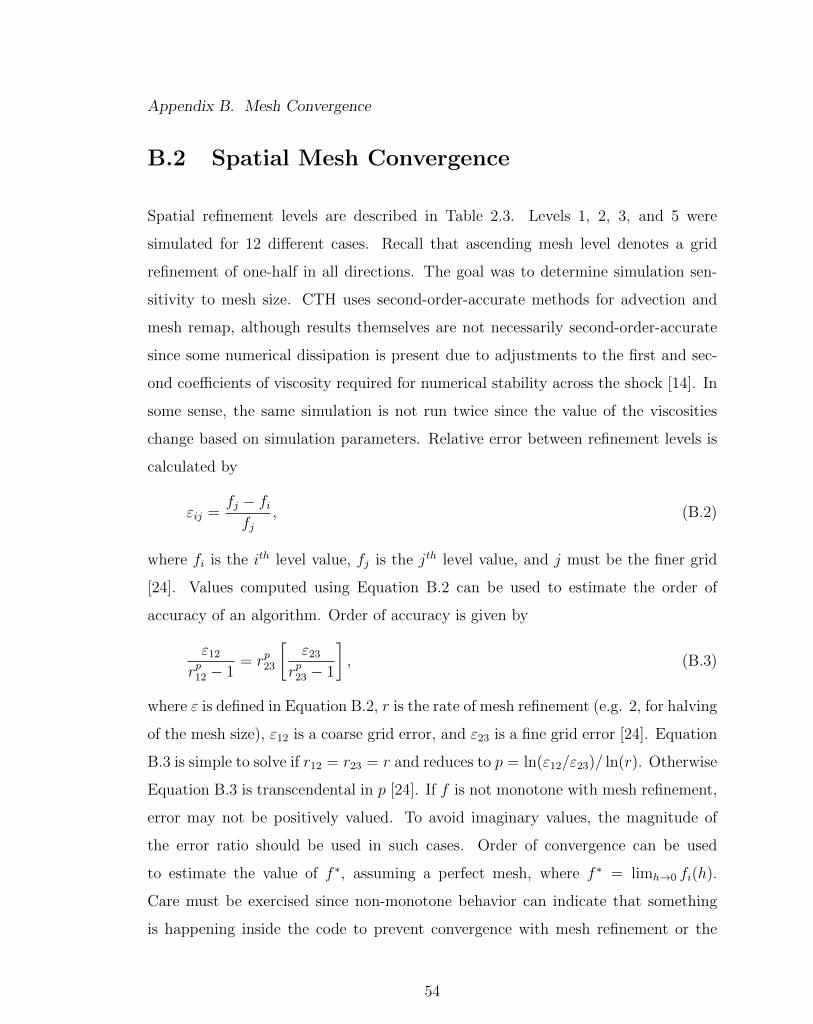
Appendix B. Mesh Convergence
B.2 Spatial Mesh Convergence
Spatial refinement levels are described in Table 2.3. Levels 1, 2, 3, and 5 were
simulated for 12 different cases. Recall that ascending mesh level denotes a grid
refinement of one-half in all directions. The goal was to determine simulation sen-
sitivity to mesh size. CTH uses second-order-accurate methods for advection and
mesh remap, although results themselves are not necessarily second-order-accurate
since some numerical dissipation is present due to adjustments to the first and sec-
ond coefficients of viscosity required for numerical stability across the shock [14]. In
some sense, the same simulation is not run twice since the value of the viscosities
change based on simulation parameters. Relative error between refinement levels is
calculated by
εij =fj − fifj
, (B.2)
where fi is the ith level value, fj is the jth level value, and j must be the finer grid
[24]. Values computed using Equation B.2 can be used to estimate the order of
accuracy of an algorithm. Order of accuracy is given by
ε12rp12 − 1
= rp23
[ε23
rp23 − 1
], (B.3)
where ε is defined in Equation B.2, r is the rate of mesh refinement (e.g. 2, for halving
of the mesh size), ε12 is a coarse grid error, and ε23 is a fine grid error [24]. Equation
B.3 is simple to solve if r12 = r23 = r and reduces to p = ln(ε12/ε23)/ ln(r). Otherwise
Equation B.3 is transcendental in p [24]. If f is not monotone with mesh refinement,
error may not be positively valued. To avoid imaginary values, the magnitude of
the error ratio should be used in such cases. Order of convergence can be used
to estimate the value of f ∗, assuming a perfect mesh, where f ∗ = limh→0 fi(h).
Care must be exercised since non-monotone behavior can indicate that something
is happening inside the code to prevent convergence with mesh refinement or the
54

Appendix B. Mesh Convergence
model is constructed incorrectly [24]. We define h to be the step size in the spatial
discretization. After running 3 different mesh sizes to calculate p, f ∗ can be directly
calculated by [24]
f ∗ = f3 +f3 − f2rp − 1
. (B.4)
Equation B.4 performs well for both monotone and non-monotone values of f . How-
ever if p → 0, the extrapolation to f ∗ is suspect since the method becomes discon-
tinuous. This is shown in Table B.4 where the φ = 25.6 case extrapolates to a value
far away from what is expected. Values in Tables B.2, B.3, and B.4 were used to
create Figures B.2, B.3, and B.4 that present error in shock speed, pressure, and
temperature relative to f ∗ plotted as ln(|ε|) versus ln(∆x).
A level 5 set of simulations was run since the values in Table B.2 are non-monotonic.
The sets of estimated p values were worse than the level 3 case but the shock speed
values were very similar to the level 1, 2, and 3 cases. Thus it was determined that
the first and second coefficients of viscosity dominate the results and mesh refinement
could not reduce error further.
Table B.2: Shock Speed Values
φ f1 [m/s] f2 [m/s] f3 [m/s] f ∗ [m/s] p ε12 ε23
128.1 931.730 932.893 932.284 931.611 0.931 1.247e-03 6.540e-0425.6 601.383 602.298 601.722 600.744 0.667 1.518e-03 9.562e-0412.8 482.760 483.610 483.330 483.192 1.601 1.759e-03 5.798e-048.5 421.521 422.070 421.830 421.644 1.195 1.300e-03 5.680e-04
145.6 959.690 961.936 961.669 961.633 3.073 2.335e-03 2.775e-0429.1 624.794 626.138 625.785 625.659 1.928 2.146e-03 5.639e-0414.6 503.293 504.262 504.094 504.059 2.529 1.922e-03 3.329e-049.7 440.342 441.097 440.815 440.647 1.421 1.713e-03 6.397e-04
163.2 985.906 988.208 987.556 987.298 1.819 2.329e-03 6.602e-0432.6 646.261 647.794 647.256 646.964 1.508 2.367e-03 8.321e-0416.3 522.143 523.222 523.009 522.956 2.341 2.062e-03 4.071e-0410.9 457.488 458.463 458.123 457.941 1.520 2.127e-03 7.416e-04
55
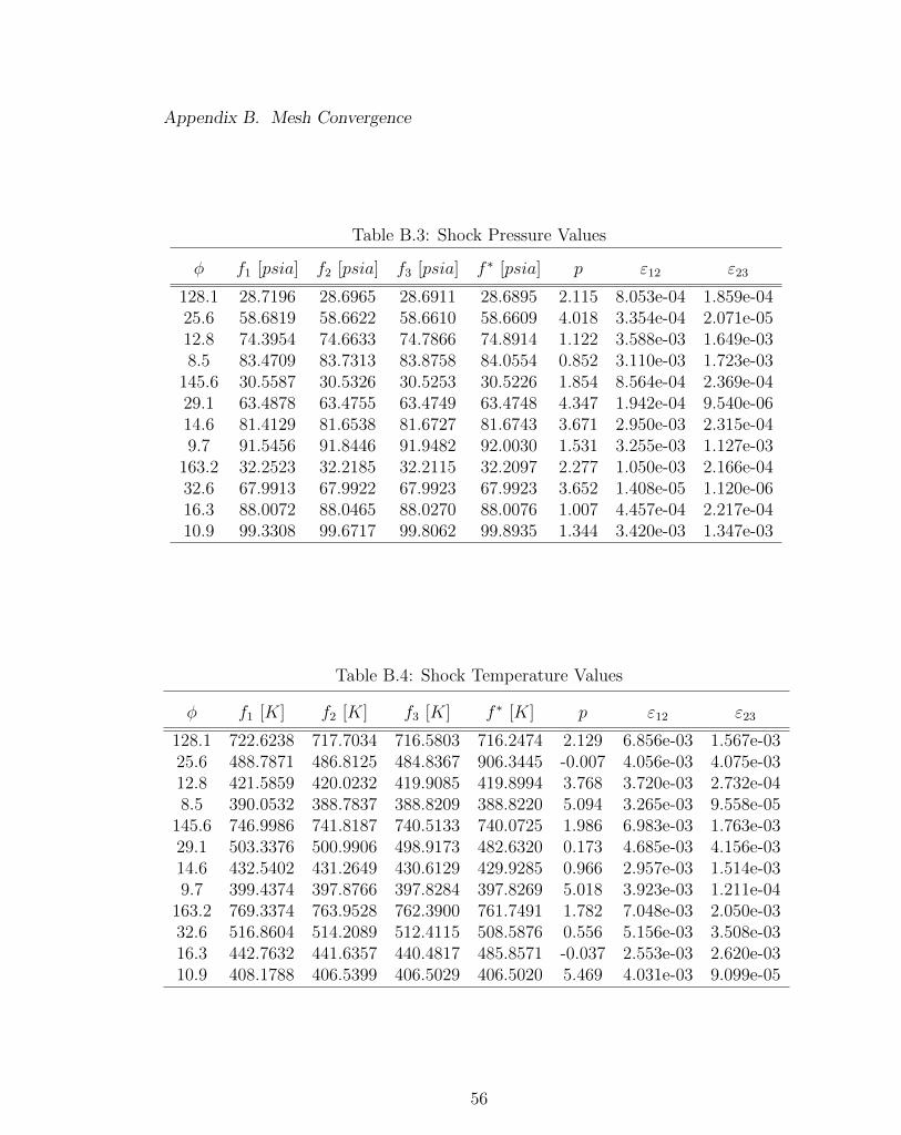
Appendix B. Mesh Convergence
Table B.3: Shock Pressure Values
φ f1 [psia] f2 [psia] f3 [psia] f ∗ [psia] p ε12 ε23
128.1 28.7196 28.6965 28.6911 28.6895 2.115 8.053e-04 1.859e-0425.6 58.6819 58.6622 58.6610 58.6609 4.018 3.354e-04 2.071e-0512.8 74.3954 74.6633 74.7866 74.8914 1.122 3.588e-03 1.649e-038.5 83.4709 83.7313 83.8758 84.0554 0.852 3.110e-03 1.723e-03
145.6 30.5587 30.5326 30.5253 30.5226 1.854 8.564e-04 2.369e-0429.1 63.4878 63.4755 63.4749 63.4748 4.347 1.942e-04 9.540e-0614.6 81.4129 81.6538 81.6727 81.6743 3.671 2.950e-03 2.315e-049.7 91.5456 91.8446 91.9482 92.0030 1.531 3.255e-03 1.127e-03
163.2 32.2523 32.2185 32.2115 32.2097 2.277 1.050e-03 2.166e-0432.6 67.9913 67.9922 67.9923 67.9923 3.652 1.408e-05 1.120e-0616.3 88.0072 88.0465 88.0270 88.0076 1.007 4.457e-04 2.217e-0410.9 99.3308 99.6717 99.8062 99.8935 1.344 3.420e-03 1.347e-03
Table B.4: Shock Temperature Values
φ f1 [K] f2 [K] f3 [K] f ∗ [K] p ε12 ε23
128.1 722.6238 717.7034 716.5803 716.2474 2.129 6.856e-03 1.567e-0325.6 488.7871 486.8125 484.8367 906.3445 -0.007 4.056e-03 4.075e-0312.8 421.5859 420.0232 419.9085 419.8994 3.768 3.720e-03 2.732e-048.5 390.0532 388.7837 388.8209 388.8220 5.094 3.265e-03 9.558e-05
145.6 746.9986 741.8187 740.5133 740.0725 1.986 6.983e-03 1.763e-0329.1 503.3376 500.9906 498.9173 482.6320 0.173 4.685e-03 4.156e-0314.6 432.5402 431.2649 430.6129 429.9285 0.966 2.957e-03 1.514e-039.7 399.4374 397.8766 397.8284 397.8269 5.018 3.923e-03 1.211e-04
163.2 769.3374 763.9528 762.3900 761.7491 1.782 7.048e-03 2.050e-0332.6 516.8604 514.2089 512.4115 508.5876 0.556 5.156e-03 3.508e-0316.3 442.7632 441.6357 440.4817 485.8571 -0.037 2.553e-03 2.620e-0310.9 408.1788 406.5399 406.5029 406.5020 5.469 4.031e-03 9.099e-05
56

Appendix B. Mesh Convergence
-1.5 -1 -0.5 0 0.5-9
-8
-7
-6
-5
-1.5 -1 -0.5 0 0.5-11
-10
-9
-8
-7
-6
-1.5 -1 -0.5 0 0.5-10
-9
-8
-7
-6
Figure B.2: Shock Speed Logarithmic Error of Mesh Levels 1, 2, and 3
57

Appendix B. Mesh Convergence
-1.5 -1 -0.5 0 0.5-14
-12
-10
-8
-6
-4
-1.5 -1 -0.5 0 0.5-15
-10
-5
-1.5 -1 -0.5 0 0.5-20
-15
-10
-5
Figure B.3: Shock Pressure Logarithmic Error of Mesh Levels 1, 2, and 3
58

Appendix B. Mesh Convergence
-1.5 -1 -0.5 0 0.5-15
-10
-5
0
-1.5 -1 -0.5 0 0.5-15
-10
-5
0
-1.5 -1 -0.5 0 0.5-15
-10
-5
0
Figure B.4: Shock Temperature Logarithmic Error of Mesh Levels 1, 2, and 3
59

Appendix C
Algorithms
In order to make the process of computing Us, Ps, and Ts tractable, MATLAB
scripts were used. This appendix briefly outlines how it was done and shows sample
calculations.
C.1 Calculating Us
Computation of Us depended on an analogue of an x-t diagram. CTH outputs
particle velocity at a tracer in the hscth file. The script simply looked to see when
velocity at the tracer was greater than zero (0) and recorded the time from the hscth
time history column. This reduces to an overdetermined system since we desire a fit
of the form x = Us · t + b and four tracers were used. Computing the shock speed
was a matter of solvingt1 1
t2 1
t3 1
t4 1
Usb
=
161.985
233.105
330.895
402.015
, (C.1)
60

Appendix C. Algorithms
where ti is the shock arrival time in seconds at the ith tracer and the right hand
side represents shock tube lengthwise tracer locations in centimeters. The value of
b is not used directly in computing Us, but not forcing the fit to pass through zero
improves the quality of the fit. Correlations were checked as a way to see how well
the speed was resolved from the data. Every correlation value was unity, indicating
expected shock speed behavior.
C.2 Calculating Ps and Ts
When the shock front passes it induces pressure and temperature spikes that can be
determined using numerical derivatives. A centered-difference scheme was used at
each tracer. The temporal derivative is given by
df
dt≈ f i+1 − f i−1
2∆t, (C.2)
where f is the quantity of interest and t is time. The derivative was maximum
when the shock passed. Thus, finding the time corresponding to the maximum
derivative value allowed the MATLAB script to find the maximum shock pressure
and temperature. An example of shock pressure is shown in Figure C.1 where the
shock is nice and crisp. Slight amounts of ringing are observed on the expansion at
tracers 1 and 2. However, checks were performed by hand to show that the script
was not fooled by the presence of slight oscillations. For shock temperature shown in
Figure C.2, the temperature spikes due to the shock but then rapidly drops due to
the expansion of the gases following the shock. Again, the shock front is sharp and
well defined allowing for easy calculation of numerical derivatives to find maximum
temperatures.
61
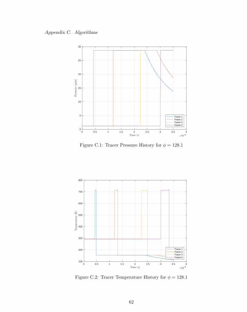
Appendix C. Algorithms
0 0.5 1 1.5 2 2.5 3 3.5 4Time [s] #10 -3
0
5
10
15
20
25
30
Pre
ssure
[psia]
Tracer 1Tracer 2Tracer 3Tracer 4
Figure C.1: Tracer Pressure History for φ = 128.1
0 0.5 1 1.5 2 2.5 3 3.5 4Time [s] #10 -3
100
200
300
400
500
600
700
800
Tem
per
atu
re[K
]
Tracer 1Tracer 2Tracer 3Tracer 4
Figure C.2: Tracer Temperature History for φ = 128.1
62

References
[1] I. Trueba Monje and J. H. Yoo, “Investigation of Dalton’s Law and Amagat’sLaw for Mixtures Using Shock Wave Propagation,” AIAA Region IV StudentConference Paper, April 2016.
[2] G. D. Wyss and K. H. Jorgensen, “A Users’s Guide to LHS: Sandia’s LatinHypercube Sampling Software,” Software Documentation SAND98-0210, SandiaNational Laboratories, 1998.
[3] K. W. Woo and S. I. Yeo, “Dalton’s Law vs. Amagat’s Law for the Mixtureof Real Gases,” The SNU Journal of Education Research, vol. 5, pp. 127–134,1995.
[4] G. J. Van Wylen and R. E. Sonntag, Fundamentals of Classical Thermodynam-ics. Hoboken, NJ: Wiley, 2nd ed., 1973. pp. 405-420,431-476.
[5] D. Li, V. Sankaran, J. W. Lindau, and C. L. Merkle, “A Unified ComputationalFormulation for Multi-Component and Multi-Phase Flows,” AIAA Paper 2005-1391, January 2005.
[6] C. L. Merkle, J. Y. Sullivan, P. E. O. Buelow, and V. Sankaran, “Computation ofFlows with Arbitrary Equations of State,” AIAA Journal, vol. 36, pp. 515–521,April 1998.
[7] P. S. Tow, “Evidence of Validity of Amagat’s Law in Determining Compressibil-ity Factors for Gaseous Mixtures under Low and Moderate Pressures,” Journalof Physical Chemistry, vol. 68, pp. 2021–2023, July 1964.
[8] G. A. Bird, “The Structure of Normal Shock Waves in a Binary Gas Mixture,”Journal of Fluid Mechanics, vol. 31, no. 4, pp. 657–668, 1968.
[9] F. S. Sherman, “Shock-wave Structure in Binary Mixtures of Chemically InertPerfect Gases,” Journal of Fluid Mechanics, vol. 8, no. 3, pp. 465–480, 1960.
63

References
[10] J. A. Beattie, “The Computation of the Thermodynamic Properties of RealGases and Mixtures of Real Gases,” in Symposium on Thermodyanmics andMolecular Structure of Solutions, September 1948.
[11] J. A. Beattie, “A Rational Basis for the Thermodynamic Treatment of RealGases and Mixtures of Real Gases,” Physical Review, vol. 36, no. 240, pp. 132–145, 1930.
[12] M. Hobbs, M. R. Baer, and B. C. McGee, “JCZS: An Intermolecular PotentialDatabase for Performing Accurate Detonation and Expansion Calculations,”Propellants, Explosives, Pyrotechnics, vol. 24, pp. 269–279, 1999.
[13] H. B. Callen, Thermodynamics and an Introduction to Thermostatistics. NewYork, NY: Wiley, 2nd ed., 1985. pp. 35-39.
[14] J. M. McGlaun, S. L. Thompson, and M. G. Elrick, “CTH: A Three-DimensionalShock Wave Physics Code,” International Journal of Impact Engineering,vol. 10, pp. 351–360, 1990.
[15] E. Clapeyron, “Memoire sur la puissance de la chaleur,” Journal de l’EcolePolytechnique (in French), vol. XIV, pp. 153–190, 1834.
[16] R. D. Cowan and W. Fickett, “Calculation of the Detonation Properties ofSolid Explosives with the Kistiakowski-Wilson Equation of State,” The Journalof Chemical Physics, vol. 24, no. 5, pp. 932–939, 1956.
[17] S. Itoh, H. Hamashima, K. Murata, and Y. Kato, “Determination of JWL Pa-rameters from Underwater Explosion Test,” in 12th International DetonationSymposium, vol. 281, 2002.
[18] E. Lee, M. Finger, and W. Collins, “JWL Equation of State Coefficients for HighExplosives,” Technical Report UCID-16189, Lawrence Livermore Laboratory,1973.
[19] M. Cowperthwaite and W. Zwisler, “The JCZ Equations of State for Detona-tion Products and Their Incorporation in the TIGER Code,” Sixth Symposium(International) on Detonation, no. ACR-221, pp. 162–172, 1976.
[20] B. McGee, M. Hobbs, and M. Baer, “Exponential 6 Parametrization for theJCZ3-EOS,” Sandia Report SAND98-1191, Sandia National Laboratories, 1998.
[21] C. L. Mader, “Detonation Properties of Condensed Explosives Computed Usingthe Becker-Kistiakowsky-Wilson Equation of State,” Technical Report LA-2900,Los Alamos Scientific Laboratory, 1963.
64

References
[22] E. Lee, H. Hornig, and J. Kury, “Adiabatic Expansion of High Explosive Det-onation Products,” Technical Report UCRL-50422, Lawrence Radiation Labo-ratory, 1968.
[23] S. Lyon and J. Johnson, “SESAME: The Los Alamos National Laboratory Equa-tion of State Database,” Technical Report LA-UR-92-3407, Los Alamos NationalLaboratory, 1992.
[24] P. J. Roache, Verification and Validation in Computational Science and Engi-neering. Albuquerque, NM: Hermosa Publishers, 2009. pp. 109-131.
[25] R. D. Zucker and O. Biblarz, Fundamentals of Gas Dynamics. Hoboken, NJ:Wiley, 2nd ed., 2002. pp. 147-158.
[26] E. N. Harstad, “CTH Shock Physics.” http://www.sandia.gov/CTH/. Ac-cessed: 15 March 2017.
[27] N. Tsoulfanidis and S. Landsberger, Measurement and Detection of Radiation.Boca Raton, FL: CRC Press, 3rd ed., 2011. pp. 17-58.
[28] J. M. Bland and D. G. Altman, “Measurement Error,” BMJ, vol. 312, no. 7047,p. 1654, 1996.
[29] M. D. Mckay, R. J. Beckman, and W. J. Conover, “A Comparison of ThreeMethods for Selecting Values of Input Variables in the Analysis of Output froma Computer Code,” Technometrics, vol. 42, pp. 55–61, 2000.
[30] M. S. Weitzman, “Measures of Overlap of Income Distributions of White andNegro Families in the United States,” U.S. Government Printing Office, vol. 22,pp. 1–37, 1970.
[31] T. E. Clemmons and E. L. Bradley, “A Nonparametric Measure of the Overlap-ping Coefficient,” Computational Statistics and Data Analysis, vol. 34, pp. 51–61, 2000.
65