A thermodynamic model for predicting mineral reactivity in ...downloads.olisystems.com/.../CO2-salt-water.pdf · Phase equilibria in mixtures containing carbon dioxide, water,

Chemical Geology 322–323 (2012) 151–171

Contents lists available at SciVerse ScienceDirect

Chemical Geology

j ourna l homepage: www.e lsev ie r .com/ locate /chemgeo

A thermodynamic model for predicting mineral reactivity in supercritical carbondioxide: I. Phase behavior of carbon dioxide–water–chloride salt systems acrossthe H2O-rich to the CO2-rich regions

Ronald D. Springer a, Zheming Wang b, Andrzej Anderko a,⁎, Peiming Wang a, Andrew R. Felmy b

a OLI Systems Inc., 108 The American Rd., Morris Plains, NJ 07950, USAb Pacific Northwest National Laboratory, 902 Battelle Blvd, Richland, WA 99352, USA

⁎ Corresponding author. Tel.: +1 973 539 4996x25;E-mail address: [email protected] (A. Ande

0009-2541/$ – see front matter © 2012 Elsevier B.V. Alldoi:10.1016/j.chemgeo.2012.07.008

a b s t r a c t
a r t i c l e i n f o
Article history:Received 22 March 2012Received in revised form 4 July 2012Accepted 7 July 2012Available online 15 July 2012

Editor: J. Fein

Keywords:Supercritical carbon dioxideChloride saltsThermodynamic modelingMixed-solvent electrolyte modelMineral reactivity

Phase equilibria in mixtures containing carbon dioxide, water, and chloride salts have been investigated using acombination of solubility measurements and thermodynamic modeling. The solubility of water in the CO2-richphase of ternary mixtures of CO2, H2O and NaCl or CaCl2 was determined, using near infrared spectroscopy, at90 atm and 40 to 100 °C. These measurements fill a gap in the experimental database for CO2–water–saltsystems, for which phase composition data have been available only for the H2O-rich phases. A thermodynamicmodel for CO2–water–salt systems has been constructed on the basis of the previously developedMixed-SolventElectrolyte (MSE) framework, which is capable ofmodeling aqueous solutions over broad ranges of temperatureand pressure, is valid to high electrolyte concentrations, treats mixed-phase systems (with both scCO2 andwaterpresent) and can predict the thermodynamic properties of dry and partially water-saturated supercritical CO2

over broad ranges of temperature and pressure. Within the MSE framework the standard-state properties arecalculated from the Helgeson–Kirkham–Flowers equation of state whereas the excess Gibbs energy includes along-range electrostatic interaction term expressed by a Pitzer–Debye–Hückel equation, a virial coefficient-type term for interactions between ions and a short-range term for interactions involving neutral molecules.The parameters of the MSE model have been evaluated using literature data for both the H2O-rich and CO2-richphases in the CO2–H2O binary and for the H2O-rich phase in the CO2–H2O–NaCl/KCl/CaCl2/MgCl2 ternary andmulticompontent systems. The model accurately represents the properties of these systems at temperaturesfrom 0 °C to 300 °C and pressures up to ~4000 atm. Further, the solubilities of H2O in CO2-rich phases that arepredicted by the model are in agreement with the new measurements for the CO2–H2O–NaCl and CO2–H2O–CaCl2 systems even though the new data were not used in the parameterization of the model. Thus, the modelcan be used to predict the effect of various salts on the water content and water activity in CO2-rich phases onthe basis of parameters determined from the properties of aqueous systems. Given the importance of water ac-tivity in CO2-rich phases for mineral reactivity, the model can be used as a foundation for predicting mineraltransformations across the entire CO2/H2O composition range from aqueous solution to anhydrous scCO2. An ex-ample application using the model is presented which involves the transformation of forsterite to nesquehoniteas a function of temperature and water content in the CO2-rich phase.

© 2012 Elsevier B.V. All rights reserved.

1. Introduction

Capture and storage of carbon dioxide in geologic formations repre-sents one of the most promising options for mitigating the impact ofgreenhouse gases on global warming, owing to the potentially large ca-pacity of these formations and their broad regional availability (Bachu,2002; Bachu and Adams, 2003; Benson and Surles, 2006; Bachu, 2008).As a result, it is important to predict the interactions of carbon dioxidewith mineral phases as they relate to geologic disposal of CO2 and the

fax: +1 973 539 5922.rko).

rights reserved.

development of mineral carbonation technologies. This can be a daunt-ing challenge given that carbon dioxide could be a supercritical fluid(T>31.1 °C and P>72.9 atm) (Regnault et al., 2005; Garcia et al.,2010), high partial pressures of carbon dioxide can result in significantformation of carbonic acid (Giammar et al., 2005; Suto et al., 2007;King et al., 2010), and H2O dissolved in supercritical CO2 can be highlyreactive (Regnault et al., 2005; Kwak et al., 2010, 2011). Although thereactivity of CO2-containing aqueous solutions, hereafter termed thewater-rich phase, is well documented (Giammar et al., 2005; Regnaultet al., 2005; Hanchen et al., 2006; Lin et al., 2008; Prigiobbe et al., 2009;Garcia et al., 2010; King et al., 2010; Daval et al., 2011; Guyot et al.,2011), the reactivity of H2O dissolved in scCO2, hereafter termed the

http://dx.doi.org/10.1016/j.chemgeo.2012.07.008

mailto:[email protected]

http://dx.doi.org/10.1016/j.chemgeo.2012.07.008

http://www.sciencedirect.com/science/journal/00092541

152 R.D. Springer et al. / Chemical Geology 322–323 (2012) 151–171

CO2-rich phase, has been largely ignored (McGrail et al., 2009; Kwak etal., 2010, 2011). The importance of H2O reactivity in the CO2-rich phaseresults from several factors. First, although the solubility of H2O inscCO2 is low (b1% by mass) the total chemical potential of H2O in theCO2-rich phase will be the same as that of H2O in the water-rich phaseif they are in equilibrium (thermodynamic phase equilibrium condition).In addition, scCO2 is highly diffusive owing to its low viscosity. Hence, ingeologic disposal, the scCO2-rich phase is likely to permeate the overly-ing repository cap rock pore network (Nordbotten and Celia, 2006) en-hancing the importance of the reactivity of the CO2-rich phase ingeologic systems. In addition, the migrating scCO2, which initially canbe anhydrous, has the potential to extract water from the formation, in-creasing theelectrolyte concentration of the remainingwater-rich phase.As a result, in order to model the full range of mineral reactivity relatedto both the disposal of scCO2 in geologic systems and the developmentofmineral carbonation technologies, a thermodynamic approach is nec-essary that can accurately represent the chemical equilibria in both thewater-rich and the CO2-rich phases over broad ranges of temperature,pressure, and electrolyte composition.

In view of the importance of the CO2–water–salt systems in geo-chemistry and chemical and petroleum engineering, various compu-tational models have been developed to represent the propertiesof such systems. In general, these models fall into two distinctcategories:

(1) γ–φ models, in which an activity coefficient formulation isused to reproduce the behavior of aqueous solutions whereasan equation of state provides the fugacity coefficients of com-ponents in the gas phase and

(2) φ–φ models, in which a homogeneous equation of state isused to reproduce the properties of both the liquid and gasphases.

The existing γ–φmodels are focused primarily on reproducing thesolubility of CO2 in water and aqueous solutions of selected salts. Inparticular, Barta and Bradley (1985), Rumpf et al. (1994), Duan andSun (2003), Duan et al. (2006) and Akinfiev and Diamond (2010) de-veloped CO2 solubility models using the well-known Pitzer (1973)activity coefficient formulation for the aqueous phase. Alternatively,the scaled particle theory of electrolyte effects was used by Li andNghiem (1986). Spycher and Pruess (2005) presented a model for cal-culating the mutual solubilities of the aqueous and CO2 phases using thePitzer (1973) activity coefficients. Salari et al. (2011) developed a modelfor estimating the water content of CO2 phases. Furthermore, the γ–φmethods have been combined with speciation calculations by Li andDuan (2007) and Li and Duan (2011).

The φ–φ approaches have been constructed either by incorporat-ing electrolyte-specific terms into nonelectrolyte equations of stateor by combining a classical equation of state with an excess Gibbs en-ergy model for electrolytes. The former approach was adopted by Jinand Donohue (1988), Harvey and Prausnitz (1989) and Ji et al. (2005)using the mean spherical approximation theory to account for elec-trostatic interactions of ions. Tan et al. (2008) reviewed models ofthis type that are based on the SAFT (Statistical Associating Fluid The-ory) equation of state whereas Lin et al. (2007) reviewed those basedon cubic and other equations of state. In an alternative approach, Liet al. (2001) and Kiepe et al. (2002) combined a cubic equation ofstate with a group contribution-based activity coefficient model forelectrolytes. Additionally, the φ–φ approaches have been shown to bemost appropriate for high-temperature systems (i.e., above ca. 300 °C),in which electrolytes exist primarily in the form of ion pairs (Anderkoand Pitzer (1993), Duan et al. (2003)).

The γ–φ and φ–φ approaches have their advantages and disadvan-tages. In principle, the φ–φ approach is more appropriate for systemsthat transition from the subcritical to supercritical range because itcan handle the vapor-liquid critical behavior, at least within the limita-tions of classical equations of state. Also, it can reproduce volumetric

properties simultaneously with phase equilibria. However, it is muchmore computationally intensive because the solution of phase equilibri-um conditions must be accompanied by solving the equation of state ineach phase. The γ–φmethods, while much less computationally inten-sive, impose a division of the phase space into gas-like and liquid-likeregions even when such a division is not physically rigorous. However,the γ–φmethods are much more amenable to integration with specia-tion and chemical equilibrium calculations. This is particularly impor-tant for modeling the interactions between minerals and CO2-bearingfluid phases, which is the ultimate objective of this work. Therefore,the γ–φ approach is more appropriate here.

Themain thrust of this study is to develop amodel that not only pre-dicts the solubility of CO2 in water-rich phases and of water in CO2-richphases but can also be used to calculate chemical equilibria involvingCO2-rich phases. This requires developing a thermodynamic modelthat can handle (1) aqueous solutions over broad ranges of temperatureand pressure up to the high electrolyte concentrations found in subsur-face brines, and (2) mixed-phase systems (with both scCO2 and waterpresent) that range from dry to partially water-saturated scCO2 overwide ranges of temperature and pressure and include high electrolyteconcentrations, which can occur when anhydrous CO2 is disposed ofand acquires water from the formation. Another requirement is thegenerality of themodel and the ease of its extension tomulticomponentsystems containingmultiple solutes and solid phases in the presence ofone or two liquid phases and/or a gas phase. These requirements aresatisfied by the previously developed Mixed-Solvent Electrolyte(MSE) model (Wang et al., 2002), which has been designed in theγ–φ framework for the simultaneous calculation of phase andchemical equilibria in systems containing strong and weak electro-lytes in aqueous, non-aqueous and mixed solvents. This model hasbeen shown to be applicable to mixtures ranging from infinite dilutionto the fused salt limit over wide ranges of temperatures (Anderko et al.,2002;Wang et al., 2004, 2006; Gruszkiewicz et al., 2007; Kosinski et al.,2007; Wang et al., 2010). The use of a mole fraction basis within MSE(rather thanmolality) also allows the mathematical algorithm for solv-ing the phase and chemical equilibrium equations to be stable at thevery high concentrations which can occur as electrolyte solutions dryin contact with anhydrous scCO2.

In this contribution, we extend the MSE model to CO2-dominatedsystems at high chloride concentrations, temperatures and pressuresthat are of importance in the disposal of scCO2 in subsurface systemsas well as in optimizing the overall mineral carbonation process in in-dustrial systems (Hanchen et al., 2008; Zhao et al., 2010; Guyot et al.,2011). We also present new measurements of H2O concentrations inscCO2-rich phases that are in equilibrium with aqueous solutionscontaining variable NaCl and CaCl2 amounts. These measurementsprovide a stringent test of the validity of the thermodynamic model,which is intended to span the H2O-rich and CO2-rich regions. Chloride-containing systems have been chosen for the initial model developmentsince chloride is a primary contributor to expected brine composi-tions in natural systems (Duan et al., 1995; Duan and Sun, 2003;Spycher and Pruess, 2005). The MSE model parameters for theH2O-rich phase are developed on the basis of the existing solubilitydata in chloride-containing systems as well as the mutual solubil-ities in the CO2–H2O binary system over a broad range of CO2 partialpressures. Thus, the model for the CO2-rich phase is anchored by theH2O solubility data in CO2 and the effect of chloride salts is evaluat-ed from the properties of the H2O-rich phases, for which relativelyabundant experimental data are available. Then, the performanceof the model is evaluated against new measurements, performedas part of this study, of the solubility of H2O in scCO2 in the presenceof concentrated NaCl and CaCl2 brines. Finally, an example applicationis given involving thermodynamic predictions for the transformationof forsterite to nesquehonite in variably wet scCO2, illustrating the im-portance of modeling the interactions of silicates and the CO2-richphase even at low water content.

153R.D. Springer et al. / Chemical Geology 322–323 (2012) 151–171

2. Experimental methods

CaCl2·2H2O, ACS Reagent grade, was purchased from Aldrich. NaCl,SigmaUltra,minimum99.5%, was purchased from Sigma. Both reagentswere used without further purification. Distilled deionized (DDI) waterwas generated using aMilliporewater filtering system. SFC grade liquidCO2 was purchased from Matheson Tri-Gas.

All experiments were performed using a modified 160 ml Parr In-struments Series 4793 GP high pressure–high temperature reactionvessel fitted with custom-made 1″ thick ¾″ x 4″ fused silica opticalwindows. The reaction vessel was pressurized using an ISCO model260D syringe pump. Multiple two-way valves and a bleeding valvewere built into the system to allow the vessel to be pressurized anddepressurized without back-flow to the CO2 supply line along withan in-line rupture disk (Fike Corporation) for safety. The pressureand temperature conditions of the system were monitored using anin-line pressure transmitter (Druck model PTX 500) and four T-typethermocouples (Newport) located at different positions inside the reac-tor to allow accurate reading of the cell temperature. All the tempera-ture and pressure sensors were interfaced to a 16-bit A/D converter(Measurement Computing model PCI-DAS1602/16) mounted in a per-sonal computer that displayed and recorded temperature and pressuredata at 32 Hz. Amagnetic stir bar was placed at the bottomof the vesseland a home-made stirrer was placed beneath the reactor to aid mixingof water and scCO2.

Near-infrared (NIR) spectra weremeasuredwith a Bruker IFS66 spec-trometer equipped with a glow bar and DTG detector for mid-IR and atungsten light source and a silicon diode detector for NIR spectra range.Spectra were recorded over the range 5000–12,000 cm−1 with a resolu-tion of 4 cm−1. The interferometer was scanned at a rate of 1.00 cm/s,and 32 scans were co-added for each spectrum. For spectral acquisitionunder a specific set of experimental conditions, the reactor was purgedwith dry N2 for at least 30 min at the desired temperature and a back-ground spectrum was recorded. After introduction of the aqueous solu-tion placed at the bottom of the reaction vessel, the cell lid was closedand tightened immediately to avoid loss of water vapor. Cell pressuriza-tion with scCO2 was initiated and sample spectrum was recorded every15 min automatically. To avoid over-pressurization, the cell pressuriza-tion with scCO2 was carried out with small pressure increments above1200 psi, allowing scCO2 thermal equilibration with the reactor. ThescCO2-water/salt solution mixture was mildly stirred initially for a mini-mum of 30 min to aid water dissolution. Spectral acquisition was endedwhen the reaction cell reaches temperature/pressure equilibrium andthe spectra were stabilized for the duration of at least an hour.

The presented spectra are the average of a minimum of three consec-utive spectra after spectral stabilization. After baseline corrections, the av-erage absorbance of theNIR spectra in the range from7100 to 7500 cm−1

was used to calculate the dissolved water concentrations.

3. Thermodynamic model

3.1. Computational framework

The derivation of the Mixed-Solvent Electrolyte (MSE) thermody-namic framework was described in previous studies (Wang et al.,2002, 2006). In order to apply it to CO2-containing systems over wideranges of pressure and temperature, we modify the MSE model by in-troducing pressure dependence into selected interaction parametersin the activity coefficient formulation. In this section,we briefly summa-rize the model and define the parameters that need to be evaluated onthe basis of experimental data.

In the MSE model, the chemical potential of a species i in a liquidphase is calculated as

μLi ¼ μL;0;x

i T; Pð Þ þ RT ln xiγx;�i T ; P; xð Þ ð1Þ

where μiL,0,x(T, P) is the standard-state chemical potential expressedon the mole fraction basis, xi is the mole fraction, and γi

x, *(T, P, x) isthe unsymmetrically normalized, mole fraction-based activity coeffi-cient. The mole fraction-based standard-state chemical potential isrelated to the well-known molality-based standard-state chemicalpotential by (Wang et al., 2002):

μL;0;xi T; Pð Þ ¼ μL;0;m

i T; Pð Þ þ RT ln1000MH2O

ð2Þ

where MH2O is the molecular weight of water. The molality-basedstandard-state chemical potential is calculated as a function of tem-perature and pressure from the Helgeson–Kirkham–Flowers (HKF)equation of state (Helgeson et al., 1974a, 1974b, 1976, 1981; TangerandHelgeson, 1988). The parameters of the HKF equation are availablefor various species from Shock and Helgeson (1988), Shock et al.(1989), and Johnson et al. (1992). For water, the standard-state chem-ical potential is defined as that of purewater and is calculated from theHaar–Gallagher–Kell equation of state (Haar et al., 1984).

The activity coefficients in Eq. (1) are obtained from an expressionfor the excess Gibbs energy, which is expressed as a sum of three con-tributions:

Gex

RT¼ Gex

LR

RTþ Gex

II

RTþ Gex

SR

RTð3Þ

where GLRex represents the contribution of long-range electrostatic

interactions, GIIex accounts for specific ionic (ion-ion and ion-molecule)

interactions, and GSRex is a short-range contribution resulting from inter-

molecular interactions. The long-range interaction contribution is calcu-lated from the Pitzer–Debye–Hückel formula (Pitzer, 1980) expressed interms of mole fractions and symmetrically normalized, i.e.,

GexLR

RT¼ − ∑

ini

� �4AxIxρ

ln1þ ρI1=2x

∑i xi 1þ ρ I0x;i� �1=2� �

0BB@

1CCA ð4Þ

where the sum is over all species, Ix is the mole fraction-based ionicstrength, Ix,i0 is defined as the ionic strength in the limiting case whenxi=1, i.e., Ix,i0 =0.5zi2; ρ is assigned a universal dimensionless value (ρ=14.0), and Ax is given by

Ax ¼13

2πNAdsð Þ1=2 e2

4πε0εskBT

!3=2

ð5Þ

where ds and εs are the molar density and dielectric constant of the sol-vent, respectively.

The specific ion-interaction contribution is calculated from anionic strength-dependent, symmetrical second virial coefficient-typeexpression (Wang et al., 2002):

GexII

RT¼ − ∑

ini

� �∑i∑jxixjBij Ixð Þ ð6Þ

where Bij(Ix)=Bji(Ix), Bii=Bjj=0, and the ionic strength dependenceof Bij is given by

Bij Ixð Þ ¼ bij þ cij exp −ffiffiffiffiffiffiffiffiffiffiffiffiffiffiffiIx þ a1

p� �ð7Þ

where bij and cij are binary interaction parameters and a1 is set equalto 0.01. The parameters bij and cij are calculated as functions of tem-perature as

bij ¼ b0;ij þ b1;ijT þ b2;ij=T þ b3;ijT2 þ b4;ij lnT ð8Þ


cij ¼ c0;ij þ c1;ijT þ c2;ij=T þ c3;ijT2 þ c4;ij lnT ð9Þ

The coefficients bk,ij (k=0, …, 4) and ck,ij (k=0,…, 4) are obtainedfrom the regression of experimental data. For the majority of speciespairs, i–j, the full complexity of the temperature dependence of bij andcij in Eqs. (8) and (9) is not needed, and only a limited number of coef-ficients are used.

The short-range interaction contribution is calculated from theUNIQUAC equation (Abrams and Prausnitz, 1975):

GexSR

RT¼ ∑

ini

� �∑ixi ln

φi

xiþ Z2∑iqixi ln

θiφi

� �− ∑

ini

� �∑iqixi ln ∑

jθjτij

!" #

ð10Þ

θi, φi, and τi are defined as

θi ¼qixi

∑j qjxjð11Þ

φi ¼rixi

∑j rjxjð12Þ

τji ¼ exp −ajiRT

� �ð13Þ

where qi and ri are the surface and size parameters, respectively, forthe species i, Z is a fixed coordination number (Z=10), and aij is thebinary interaction parameter between species i and j (aij≠aji). Theshort-range interaction parameters are calculated as functions oftemperature and pressure by

aij ¼ a 0ð Þij þ a 1ð Þ

ij T þ a 2ð Þij T2 þ a P0ð Þ

ij þ a P1ð Þij T þ a P2ð Þ

ij T2� �

P ð14Þ

where aij≠aji. As with the ionic interaction parameters, all coeffi-cients of Eq. (14) are usually not needed for most species pairs. Insystems containing only strong electrolytes, only the ion interactionparameters (Eqs. (8)–(9)) are needed. The short-range parameters(Eq. (14)) are introduced only for interactions involving neutralmolecules.

The activity coefficients are calculated from Eq. (3) by differenti-ation with respect to the number of moles (Pitzer, 1995). Since theactivity coefficients calculated from Eq. (3) are symmetrically nor-malized (i.e., they are equal to 1 for each pure component), theyneed to be converted to unsymmetrical normalization so that theyare based on the infinite-dilution reference state in water and canbe used in Eq. (1):

ln γx;�i ¼ ln γx

i− limxi→0xw→1

ln γxi ð15Þ

where lim xi→0xw→1

lnγxi is the value of the symmetrically-normalized

activity coefficient at infinite dilution in water, which is calculated bysubstituting xi=0 and xw=1 into the activity coefficient equations.

The chemical potential of species i in the gas phase is given by

μGi ¼ μG;0

i Tð Þ þ RT lnPyiϕi T; Pð Þ

P0 ð16Þ

where μiG,0(T) is the chemical potential of pure component i in the idealgas state, yi is the mole fraction in the gas phase, ϕi(T, P) is the fugacitycoefficient, P is the total pressure, and P0=1 atm. The μiG,0(T) term iscalculated from the ideal-gas Gibbs energy of formation, entropy andheat capacity according to standard thermodynamics (Pitzer, 1995).

For water, this term is obtained from the Haar–Gallagher–Kell equationof state (Haar et al., 1984). The fugacity coefficient is calculated from theSoave–Redlich–Kwong (SRK) equation of state (Soave, 1972):

P ¼ RTv−b

− av vþ bð Þ ð17Þ

where v is the molar volume and the parameters a and b are calculatedusing the classical quadratic mixing rules, i.e.,

a ¼ ∑i∑jxixj aiaj� �1=2

1−kij� �

ð18Þ

b ¼ ∑ixibi ð19Þ

The pure-component parameters ai and bi are calculated using thecritical properties Tc and Pc and a temperature-dependent functionα(T), which is regressed to match pure-component vapor pressures:

ai ¼ 0:42747R2T2

ci

Pciαi Tð Þ ð20Þ

bi ¼ 0:08664RTci

Pcið21Þ

The binary parameter kij in Eq. (18) is expressed as a function oftemperature as

kij ¼ k 0ð Þij þ k 1ð Þ

ij =T ð22Þ

The fugacity coefficient ϕi(T, P) is calculated from Eqs. (17)–(22)using standard thermodynamic relations (Pitzer, 1995).

The expressions for the chemical potentials of species in the liq-uid and gas phases are further used for the simultaneous calculationof phase (i.e., vapor-liquid and liquid-liquid) equilibria and chemical (orspeciation) equilibria between solution species as described by Zemaitiset al. (1986) and Rafal et al. (1995). The calculations were performedusing a phase and chemical equilibrium algorithm that is implementedin theOLI software (OLISystems, 2012). Themodel parameters reportedhere are available in the OLI software starting from version 9.0.

3.2. Determination of model parameters

The combined thermodynamic framework has been applied tomodel the phase behavior of binary and mixed CO2–Na–K–Mg–Ca–Cl–H2O systems. Table 1 summarizes the available literature sourcesfor these systems together with their temperature, pressure, andsalt content ranges.

For the binary and multicomponent Na–K–Mg–Ca–Cl–H2O sys-tems (i.e., without CO2), the MSE parameters were determined in aprevious study (Gruszkiewicz et al., 2007). These parameters ensurethat the model reproduces the phase equilibria and caloric propertiesof binary, ternary, and multicomponent mixtures from the freezingpoint up to 300 °C and from infinite dilution to the solid saturationor fused salt limit. Table 2 summarizes the parameters that determinethe thermodynamic properties of individual species in the Na–K–Mg–Ca–Cl–H2O systems (i.e., the standard partial molar Gibbs en-ergy of formation, entropy, and parameters of the HKF equation ofstate). These species include the individual ions (i.e., Na+, K+, Mg2+,Ca2+, and Cl−) and the ion pairs (i.e., MgCl2(aq) and CaCl2(aq)) thatwere taken into account in the previous study (Gruszkiewicz et al.,2007). Table 3 compiles the ionic interaction parameters (Eqs. (8)–(9))between these species.


In this study, we determine parameters to reproduce the proper-ties of the following systems:

(1) The binary system CO2–H2O(2) Ternary mixtures composed of CO2, H2O and one of the four

chloride salts, i.e., NaCl, KCl, MgCl2, and CaCl2(3) Multicomponent mixtures containing CO2, H2O and various

combinations of NaCl, KCl, MgCl2 or CaCl2.

In the first step of model development, MSE parameters have beendetermined for the CO2–H2O binary. There are a large number of ex-perimental studies that report experimental data for this system (cf.Table 1). Furthermore, critical reviews are available to guide the rela-tive weighting of experimental data for model development. The datathat are available in the low-pressure range and at temperatures upto 433 K have been reviewed by Carroll et al. (1991). The solubilitiesof CO2 in H2O have been evaluated by Crovetto (1991) at tempera-tures up to the critical point, by Diamond and Akinfiev (2003) up to100 °C and 100 MPa and by Duan and Sun (2003) up to 260 °C and200 MPa. Spycher et al. (2003) reviewed the mutual solubilities ofCO2 and H2O up to 100 °C and 60 MPa. The latter three reviews dealwith the conditions that are particularly relevant to geological se-questration. The data at higher temperatures and pressures havebeen evaluated by Mäder (1991), Mather and Franck (1992) andBlencoe et al. (2001).

In this study, we regress parameters to reproduce the experimen-tal data for temperatures ranging from 0 °C to 300 °C and pressuresup to approximately 350 MPa. The parameters are determined onthe basis of (a) solubilities of CO2 in H2O, (b) solubilities of H2O inCO2, (c) pure-component vapor-pressures of CO2 and (d) enthalpiesof mixing of CO2 and H2O. The application of the MSE model to theCO2–H2O system is constrained by the inherent characteristics ofthe γ–φ methods for calculating phase equilibria (Anderko andMalanowski, 1992). In the γ–φ methods, fluid phase equilibria canbe calculated as either vapor-liquid (VLE) or liquid-liquid (LLE) equi-libria. In the former case, the model uses separate formulations forthe two phases, i.e., Eq. (1) for the liquid phase and Eq. (16) for thevapor phase. In the latter case, Eq. (1) is used for both phases.Below the critical temperature of the lighter component (i.e., below304.12 K in the case of CO2), there is a distinct transition betweenthe VLE and LLE regions. The two regions are separated by thethree-phase vapor–liquid–liquid region and the three-phase equilib-rium pressure is, at a given temperature, very close to the vapor pres-sure of pure CO2. Above the critical temperature of CO2, there is onlyone fluid-fluid equilibrium region, which transitions smoothly from aVLE-like region to an LLE-like region as the pressure increases. How-ever, a γ–φ model still calculates phase equilibria as VLE at lowerpressures and as LLE at higher pressures. The transition betweenthese two regions becomes then arbitrary and lies on an extensionof the VLLE P vs. T curve beyond the critical temperature of CO2. How-ever, with appropriately adjusted model parameters, the VLE-like andLLE-like regions can merge seamlessly and correctly approximate thesolubility of scCO2 in the water phase and water in the scCO2 phaseacross the full pressure range of phase equilibria.

In order to reproduce the behavior of the CO2–H2O binary, theMSE model requires three kinds of parameters, i.e., (1) thestandard-state Gibbs energy of formation, entropy and HKF equationparameters for CO2(aq), (2) the interaction parameters in the formula-tion for the excess Gibbs energy (Eqs. (8) and (14)) and (3) standard-state properties of CO2 in the gas phase and the parameters of the SRKequation (Eqs. (17)–(22)). In the LLE region of the phase coexistencecurve, the properties of both phases are modeled using the liquid-phase chemical potential expression (Eq. (1)). Thus, the LLE regionis reproduced exclusively by the liquid-phase interaction parametersbecause the standard-state chemical potential drops out when Eq. (1)is applied to both coexisting phases. On the other hand, the VLEregion is represented by Eq. (1) for the liquid phase and Eq. (16) for

the gas phase. The liquid-phase properties in the VLE region dependprimarily on the standard-state properties and, to a lesser extent, onthe liquid-phase interaction parameters. The liquid-phase interactionparameters play a much lesser role here because the concentration ofCO2 in the water-rich phase is relatively low. The chemical potentialof CO2 in the gas phase depends on the SRK interaction parameters(Eq. (22)) in addition to the pure-component properties, which arefixed at their experimental values and collected in Table 4. At lowpressures, the gas phase is nearly ideal and VLE calculations dependprimarily on the standard-state properties of CO2(aq). As the pressureincreases, the gas-phase fugacity coefficients increasingly depend onthe SRK interaction coefficients. In view of the different sensitivityof the VLE and LLE regions to various model parameters, initial esti-mates of the liquid-phase interaction parameters (Eqs. (8) and(14)) have been obtained from the data in the LLE region whereasthe initial values of the SRK interaction parameters (Eq. (22)) havebeen obtained from the VLE region in the elevated pressure range.Subsequently, the parameters have been refined through a combinedoptimization using a complete set of phase equilibrium data. For theliquid-phase interaction parameters, it has been determined thatthe optimum representation of phase equilibria is obtained usingthe ionic strength-independent virial parameters Bij in the virial ex-pansion (i.e., by using only the coefficients b0,ij, b1,ij, and b2,ij inEq. (8) and setting all cij coefficients in Eq. (9) equal to zero) coupledwith the pressure-dependent UNIQUAC interaction parameters aij(i.e., by regressing the coefficients aij

(0), aij(1), aij

(P0), and aij(P1) in

Eq. (14), the last two of which impose a linear pressure dependenceon aij). The pressure dependence is necessary due to the very widepressure range of the available phase equilibrium data (up to350 MPa). For simplicity and in view of the rather small differencesin the sizes of the species considered here, the ri and qi parametersin the short-range term (Eqs. (11)–(12)) are set equal to 0.92 and1.4, respectively, for all species. The HKF equation parameters forCO2(aq) have been slightly adjusted by modifying the aHKF,1,…4 param-eters in the combined model while keeping the remaining parame-ters (i.e., cHKF,1, cHKF,2 and ω) unchanged. Table 2 includes thestandard-state properties of CO2(aq). The virial-type interaction pa-rameters between CO2 and H2O (b0,ij, b1,ij, and b2,ij) are listed inTable 3. Finally, Table 5 contains the UNIQUAC liquid-phase interac-tion parameters (aij(0), aij(1), aij(P0), and aij

(P1)) and the SRK binary param-eters (kij(0) and kij

(0)).In the second stage of parameter development, mixtures

containing chloride salts as well as CO2 and H2O have been analyzed.Table 1 summarizes the sources of experimental data that includeNaCl, KCl, MgCl2, and CaCl2 as the salt components and lists the tem-perature, pressure and salt content ranges of the data. The experi-mental data base is particularly abundant in the case of NaCl–CO2–

H2O system, for which 27 data sources have been identified. For thissystem, the experimental studies have been reviewed by Spycherand Pruess (2005) and Koschel et al. (2006). The data are also fairlyextensive for the KCl–CO2–H2O and CaCl2–CO2–H2O systems, foreach of which 11 data sources are available. For these three ternarysystems, a significant number of data sets extend well into the tem-perature and pressure ranges that are relevant to CO2 sequestration(cf. Table 1). Data for the MgCl2–CO2–H2O system are limited to asmall number of sources (i.e., three) and ambient pressures. Only afew data sets are available for mixed chloride salts. It should benoted that all of the literature data sources pertain to the water-richliquid phase and none of them deals with the carbon dioxide-richphase in the presence of salts.

Analysis of experimental data has revealed that the effect of saltson the solubility of CO2 can be reproduced using a single,temperature-independent interaction parameter b0,ij between thecations (i.e., Na+, K+, Mg2+ and Ca2+) and CO2(aq) in the virialterm (Eq. (8)). These parameters are listed in Table 3. Consideringthe wide temperature, pressure and salt concentration ranges of

Table 1Experimental data sources for the CO2–Na–K– Mg–Ca–Cl–H2O systems.

System Reference Temperature range, K Pressure range, atm Salt concentration mol∙kg−1 H2O

CO2–H2O Bunsen (1855b) 277.55–295.55 1 0Bunsen (1855a) 273.15–293.15 1 0de Khanikof and Louguinine (1867) 288.15 1–4 0Setschenow (1874) 288.35–290.25 1 0Setchenow (1879) 310.4 1 0Setchenow (1887) 288.35–296.15 1 0Setchenow (1889) 288.35 1 0Bohr and Bock (1891) 310.44–373.15 1 0Setchenow (1892) 288.35 1 0Prytz and Holst (1895) 273.15 1 0Bohr (1899) 273.25–334.55 1 0Hantzsch and Vogt (1901) 273.15–363.15 0.09–0.12 0Geffcken (1904) 288.15–298.15 1 0Findlay and Creighton (1910) 298.15 1–1.8 0Findlay and Shen (1912) 298.15 1–1.8 0Sander (1912) 293.15–375.15 25–165 0Findlay and Williams (1913) 298.15 0.35–1 0Findlay and Howell (1915) 298.15 0.35–1.3 0Kunerth (1922) 293.15–307.15 1 0Morgan and Pyne (1930) 298.15 1 0Morgan and Maass (1931) 273.15–298.15 0.1–1.1 0Kritschewski et al. (1935) 293.15–303.15 5–30 0Kobe and Williams (1935) 298.15 1 0Shedlovsky and MacInnes (1935) 298.15 1 0Zelvenskii (1937) 273.15–373.15 10–95 0Curry and Hazelton (1938) 298.15 1 0Van Slyke (1939) 295.95–298.65 1 0Wiebe and Gaddy (1939) 323.15–373.15 25–700 0Wiebe and Gaddy (1940) 285.15–313.15 25–500 0Markham and Kobe (1941) 273.35–313.15 1 0Wiebe and Gaddy (1941) 298.15 500 0Harned and Davis (1943) 273.15–323.15 1 0Stone (1943) 244.15–295.75 15–60 0Prutton and Savage (1945) 374.15–393.15 25–690 0Koch et al. (1949) 291.45–295.05 0.14–0.21 0Morrison and Billett (1952) 286.45–347.85 1 0Rosenthal (1954) 293.15 1 0Dodds et al. (1956) 273.15–393.15 0.1–700 0Houghton et al. (1957) 273.15–373.15 1–36 0Shchennikova et al. (1957) 293.15–348.15 1 0Ellis (1959) 387.15–621.15 5–160 0Garner et al. (1959) 303.15 5–20 0Malinin (1959) 473.15–603.15 100–480 0Bartels and Wrbitzky (1960) 288.15–311.15 1 0Novak et al. (1961) 284.65–350.15 0.15–1 0Austin et al. (1963) 293.15–311.15 1 0Ellis and Golding (1963) 450.15–607.15 15–75 0Tödheide and Franck (1963) 323.15–643.15 200–3550 0Takenouchi and Kennedy (1964) 383.15–623.15 100–1480 0Yeh and Peterson (1964) 298.15–318.15 1 0Takenouchi and Kennedy (1965) 423.15–623.15 100–1380 0Vilcu and Gainar (1967) 293.15–308.15 25–75 0Gerecke (1969) 288.15–333.15 1 0Matous et al. (1969) 303.15–353.15 10–40 0Onda et al. (1970a) 298.15 1 0Power and Stegall (1970) 310.15 1 0Stewart and Munjal (1970) 273.15–298.15 10–45 0Barton and Hsu (1971) 273.35–313.15 1 0Coan and King (1971) 298.15–373.15 15–50 0Hayduk and Malik (1971) 298.15 1 0Li and Tsui (1971) 273.85–303.15 1 0Murray and Riley (1971) 274.19–308.15 1 0Malinin and Savelyeva (1972) 298.15–348.15 47 0Malinin and Kurovskaya (1975) 298.15–423.15 47 0Angus (1976) 216.58–303.1 5–70 0Yasunishi and Yoshida (1979) 288.15–308.15 1 0Drummond (1981) 303.85–621.65 40–260 0Shagiakhmetov and Tarzimanov (1981) 323.15–423.15 100–790 0Won et al. (1981) 298.15 1 0Zawisza and Malesińska (1981) 323.15–473.15 1.5–55 0Burmakina et al. (1982) 298.15 1 0Cramer (1982) 306.15–486.25 8–55 0Gillespie et al. (1984) 288.71–533.15 7–200 0Briones et al. (1987) 323.15 65–170 0Nakayama et al. (1987) 298.15 35–110 0Postigo and Katz (1987) 288.15–308.15 1 0


Table 1 (continued)


DiSouza et al. (1988) 323.15–348.15 100–150 0Müller et al. (1988) 373.15–473.15 3–80 0Eremina et al. (1989) 298.15–313.15 1 0Nighswander et al. (1989) 352.85–471.25 20–100 0Oyevaar et al. (1989) 298.15 1 0Traub and Stephan (1990) 313.15 40–100 0Carroll et al. (1991) 273.15–433.15 0.5–10 0Sterner and Bodnar (1991) 494.15–608.15 480–3060 0Sako et al. (1991) 348.15–421.4 100–195 0Crovetto and Wood (1992) 623.05–642.65 175–220 0King et al. (1992) 288.15–313.15 50–240 0Mather and Franck (1992) 273.15–546.45 10–3070 0Dohrn et al. (1993) 323.15 100–300 0Ohgaki et al. (1993) 283.07–289.37 45–50 0Yang and Yuan (1993) 278.15–318.15 1 0Rumpf et al. (1994) 323.15 10–55 0Vazquez et al. (1994a) 298.15 1 0Jackson et al. (1995) 323.15–348.15 340 0Fenghour et al. (1996) 405–613 55–240 0Scharlin (1996) 273.15–433.15 1 0Teng et al. (1997) 278.15–293.15 60–290 0Zheng et al. (1997) 278.15–338.15 0.5–0.85 0Dhima et al. (1999) 344.15 100–990 0Fan and Guo (1999) 283.1 46 0Wendland et al. (1999) 281.21–304.63 40–75 0Bamberger et al. (2000) 323.15–353.15 40–140 0Blencoe et al. (2001) 573.15 270–560 0Servio and Englezos (2001) 277.05–283.15 20–40 0Kiepe et al. (2002) 313.15–393.15 1–90 0Bando et al. (2003) 303.15–333.15 100–200 0Chapoy et al. (2004) 274.14–351.31 2–90 0Li et al. (2004) 332.15 35–200 0Valtz et al. (2004) 278.22–318.23 5–80 0Koschel et al. (2006) 323.15–373.15 20–200 0

CO2–NaCl–H2O Mackenzie (1877) 279.55–295.15 1 1.3–6Setchenow (1892) 288.35 1 0.2–6.1Kobe and Williams (1935) 298.15 1 1.9–5.7Markham and Kobe (1941) 273.35–313.15 1 0.1–4Harned and Davis (1943) 273.15–323.15 1 0.2–3Rosenthal (1954) 293.15 1 1.6–5.7Ellis and Golding (1963) 445.15–603.15 25–90 0.5–2Yeh and Peterson (1964) 298.15–318.15 1 0.16Takenouchi and Kennedy (1965) 423.15–723.15 100–1380 1.1–4.3Gerecke (1969) 288.15–333.15 1 0.5–4.7Onda et al. (1970a) 298.15 1 0.5–3.2Malinin and Savelyeva (1972) 298.15–348.15 47 0.4–4.9Malinin and Kurovskaya (1975) 298.15–423.15 47 1–6.8Yasunishi and Yoshida (1979) 288.15–308.15 1 0.5–5.7Gehrig (1980) 408.15–573.15 875–2680 1.1Drummond (1981) 292.85–673.15 35–390 1–6.5Burmakina et al. (1982) 298.15 1 0.001–0.2Cramer (1982) 296.75–511.75 8–60 0.5–2Nighswander et al. (1989) 353.15–473.65 20–100 0.17He and Morse (1993) 273.15–363.15 0.04–1 0.1–6.1Rumpf et al. (1994) 313.15–433.15 5–95 4–6Vazquez et al. (1994a) 298.15 1 0.7–2.9Vazquez et al. (1994b) 293.15–308.15 1 0.7–2.9Zheng et al. (1997) 278.15–338.15 0.5–0.85 0.7–3.3Kiepe et al. (2002) 313.15–353.15 1–100 0.5–4.3Bando et al. (2003) 303.15–333.15 100–200 0.15–0.55Koschel et al. (2006) 323.15–373.15 50–200 1–3

CO2–KCl– H2O Mackenzie (1877) 281.15–295.15 1 0.9–3.9Setchenow (1892) 288.35 1 0.9–2.8Geffcken (1904) 288.15–298.15 1 0.4–1.1Findlay and Shen (1912) 298.15 1 0.25–1Markham and Kobe (1941) 273.35–313.15 1 0.1–4Gerecke (Gerecke, 1969) 288.15–333.15 1 0.5–3.3Yasunishi and Yoshida (1979) 298.15–308.15 1 0.4–4.7Burmakina et al. (1982) 298.15 1 0.001–0.2He and Morse (1993) 273.15–363.15 0.3–1 0.1–5Kiepe et al. (2002) 313.15–353.15 1–100 0.5–4Kamps et al. (2007) 313.15–433.15 5–90 1.9–4.1

CO2–MgCl2–H2O Kobe and Williams (1935) 298.15 1 4.5Yasunishi and Yoshida (1979) 288.15–308.15 1 0.15–4.4He and Morse (1993) 273.15–363.15 0.3–1 0.1–5.0

(continued on next page)

CO2–H2O


Table 1 (continued)


CO2–CaCl2–H2O Mackenzie (1877) 281.15–303.15 1 0.4–1.7Setchenow (1892) 288.35 1 0.15–5Kobe and Williams (1935) 298.15 1 6Prutton and Savage (1945) 348.65–394.15 15–700 1–3.9Malinin (1959) 473.15–623.15 100–390 1Onda et al. (1970b) 298.15 1 0.2–2.3Malinin and Savelyeva (1972) 298.15–348.15 47 0.2–4.4Malinin and Kurovskaya (1975) 373.15–423.15 47 0.9–8.8Yasunishi and Yoshida (1979) 298.15–308.15 1 0.2–5.3Eremina et al. (1989) 298.15–313.15 1 0.0025–0.025He and Morse (1993) 273.15–363.15 0.3–1 0.1–5

CO2–NaCl– KCl–H2O Yasunishi et al. (1979) 298.15 1 0.5–5CO2–NaCl–CaCl2–H2O Malinin and Savelyeva (1972) 298.15 47 1.4CO2–KCl–CaCl2–H2O Yasunishi et al. (1979) 298.15 1 0.4–3.9CO2–NaCl–KCl–CaCl2–H2O Yasunishi et al. (1979) 298.15 1 0.4–3


CO2 solubility in NaCl, KCl, and CaCl2 solutions, the simplicity of theion–CO2 interaction parameters is remarkable and can be expectedto contribute to the predictive character of the model across the fullrange of CO2 content in the liquid phase, i.e., from the H2O-rich tothe CO2-rich region. We emphasize that the new experimental datameasured in this study have not been used in the determination ofparameters. Thus, they provide a stringent test of the predictive capa-bility of the model.

4. Results and discussion

4.1. Measurement of water solubilities in scCO2

Experimental water concentrations in scCO2 in contact with solu-tions of CaCl2 and NaCl (Table 6) as a function of temperature showthe expected trends of increasing water solubility in scCO2 with in-creasing temperature and decreasing water solubility with increasingelectrolyte concentration. Two different solutions of CaCl2 and NaClwere prepared and analyzed. The first set, labeled “Sat” in Table 6,represents solutions that were saturated with the indicated electro-lyte solution at 25 °C. The second set, labeled Sat+3.0 g solid(NaCl) or Sat+2.16 g solid (CaCl2) were solutions with additionalsolid phase added to the solution prior to introducing the solution/solid slurry to the experimental system. The presence of additionalsolid was designed to insure solid/aqueous solution phase equilibri-um even as the temperature was increased. The water solubility inscCO2 was then measured for these solutions as a function of temper-ature. In the case of NaCl the measured water solubilities in scCO2

were nearly the same in both sets 1 and 2 since the solubility ofNaCl in water does not increase rapidly with temperature from 40to 100 °C. However, in the case of CaCl2 the measured water solubilitywas significantly different between sets 1 and 2 since the solubility ofCaCl2 at 25 °C is much lower (~7 m) than at 100 °C (13.6 m, see

Table 2Parameters that determine the thermodynamic properties of individual ionic and neutral spHelgeson–Kirkham–Flowers equation of state (Helgeson et al. (1974a, 1974b), Helgeson et alproperties (aHKF,1,.. 4,cHKF,1, cHKF,2, ω).

Species ΔG0f kJ⋅mol−1 S

0J⋅mol−1 K−1 aHKF,1 aHKF,2

Na+a −261.881 58.4086 0.1839 −228.5K+a −282.462 101.044 0.3559 −147.3Mg2+a −453.960 −138.100 −0.08217 −859.9Ca2+a −552.790 −56.484 −0.01947 −725.2Cl−a −131.290 56.735 0.4032 480.1MgCl2(aq)b −623.223 2.8920 0.62187 740.58CaCl2(aq)b −794.040 67.7344 0.62187 740.58CO2(aq)

c −385.974 117.57 1.50979 0.

a Parameters were obtained from Shock and Helgeson (1988) and Shock et al. (1989).b Parameters for the ion pairs were determined in a previous study (Gruszkiewicz et al.,c Parameters adjusted in this study.

Table 6). As a result, the measured water solubility in scCO2 in contactwith aqueous CaCl2 solutions is much lower in the solutions with ad-ditional solid CaCl2 than in the absence of the solid. This comparisonalso holds across the entire range of electrolyte concentrations exam-ined for both NaCl and CaCl2.

4.2. Modeling phase equilibria in aqueous H2O–CO2–Na–Ca–Cl systems

4.2.1. CO2–H2O binaryFigs. 1–3 compare the model predictions with experimental data

for the CO2–H2O binary system. Fig. 1 shows the equilibrium pressureas a function of CO2 mole fraction in the aqueous phase for five select-ed isotherms (i.e., 0, 25, 50, 100, and 150 °C). The experimental datain Fig. 1 have been assembled from various sources so that the mea-sured temperatures do not deviate from the temperatures indicatedin Fig. 1 by more than 0.2 °C. Since the solubilities of CO2 in waterhave been comprehensively reviewed by Diamond and Akinfiev(2003), Duan and Sun (2003) and Spycher et al. (2003), a criticalevaluation of the experimental data is outside of the scope of thiswork. As discussed by Duan and Sun (2003), most CO2 solubilitydata in water are consistent within approximately 7% up to 533 K and2000 atm. Therefore, Fig. 1 combines the CO2 solubility data from vari-ous sources (Table 1). The model reproduces the majority of the data(except for those of Zelvenskii (1937), Dodds et al. (1956), Vilcu andGainar (1967), Stewart and Munjal (1970), Shagiakhmetov andTarzimanov (1981) and Kiepe et al. (2002)) within the experimentalscattering for pressures up to 3500 atm.

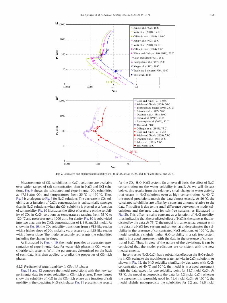
Various data sources for the solubility of H2O in CO2 show muchgreater discrepancies than those for the solubility of CO2 in H2O andthese discrepancies increase with temperature. Therefore, Figs. 2and 3 compare the calculated results with individual data sources.Fig. 2a shows the H2O solubilities in CO2 for two subcritical isotherms(i.e., 15 °C and 25 °C) and one isotherm that is above the critical point

ecies: standard partial molar Gibbs energy of formation, entropy, and parameters of the. (1976, 1981), Tanger and Helgeson (1988)) for standard partial molar thermodynamic

aHKF,3 aHKF,4 cHKF,1 cHKF,2 ω

3.256 −27260 18.18 −29,810 330605.435 −27120 7.4 −17,910 192708.39 −23900 20.8 −58,920 1537205.2966 −24792 9 −25,220 1236605.563 −28470 −4.4 −57,140 1456002.8322 −30851 23.961 32,720 −38002.8322 −30851 23.961 32,720 −3800

−109.419 0. 40.0325 88,004 −2000

2007) based on multiproperty regressions for aqueous salt solutions.

Table 3Binary parameters used in the virial interaction term (Eqs. (8)–(9)).

Species i Species j b0,ij b1,ij b2,ij b3,ij b4,ij c0,ij c1,ij c2,ij c3,ij c4,ij

Na+ Cl− 15610.63 7.964204 −357992.9 −0.003643102 −2892.662 −30086.35 −15.00973 699,848.7 0.006820989 5552.343K+ Cl− 15087.68 7.236058 −354195.6 −0.003141513 −2771.596 −26853.29 −12.85712 635,045.6 0.005649944 4927.578Mg2+ Cl− −46.0902 0.036682 −12896 8.29385e−6 0 110.429 −0.240247 11,645.2 0.000319761 0Ca2+ Cl− −95.9932 0.470226 −17370.9 −5.67551e−4 0 −0.694366 −0.421581 43,725.9 0.000791106 0Na+ K+ −93.0411 −0.234488 37002.7 5.62879e−4 0 −64.633 0.881525 −29,428.5 −0.00128594 0Na+ Mg2+ −28.8624 0.0351923 8744.27 0 0 0 0 −6373.88 0 0Na+ Ca2+ 11.2685 −0.0263793 2905.5 0 0 0 0 −6685.21 0 0K+ Mg2+ −28.2506 0.0311345 16139.0 0 0 0 0 −13,262.6 0 0K+ Ca2+ −43.804 0.0468862 23092.5 0 0 0 0 −18,687.4 0 0CaCl2(aq) Na+ −27.3022 0 17433. 0 0 0 0 0 0 0CaCl2(aq) K+ −24.2268 0 18665.2 0 0 0 0 0 0 0CaCl2(aq) H2O −9.09197 0 7761.96 0 0 0 0 0 0 0MgCl2(aq) Na+ 0 0 −11710.7 0 0 0 0 0 0 0MgCl2(aq) K+ 0 0 −9228.3 0 0 0 0 0 0 0CO2(aq) H2O −10.2134 0.0102376 783.548 0 0 0 0 0 0 0CO2(aq) Na+ −10.9006 0 0 0 0 0 0 0 0 0CO2(aq) K+ −8.51244 0 0 0 0 0 0 0 0 0CO2(aq) Mg2+ −21.1002 0 0 0 0 0 0 0 0 0CO2(aq) Ca2+ −20.4164 0 0 0 0 0 0 0 0 0


of CO2 (i.e., 40 °C). The 15 °C and 25 °C isotherms show a transitionbetween vapor–liquid and liquid–liquid equilibria at 50 and63.3 atm, respectively. The calculations are in a generally goodagreement with data from three separate literature sources for the15 °C isotherm and six sources for the 25 °C isotherm. At 40 °C, atransition is observed between the VLE-like region below ca. 100 atmand an LLE-like region above 100 atm. The calculations are in a reason-able agreement with the data of King et al. (1992) and Traub andStephan (1990).

Fig. 2b shows the results for the 50 °C and 75 °C isotherms. At 50 °C,literature data are available from seven sources. The data of Wiebe andGaddy (1939), Coan and King (1971), Briones et al. (1987), andBamberger et al. (2000) are in an excellent agreement with each otherin the VLE region and in the region of transition between the VLE-likeand LLE-like behavior. The model accurately reproduces these data.However, substantial discrepancies are observed in the LLE-like region,in which Tödheide and Franck (1963) and DiSouza et al. (1988) reportmeaningfully higher solubilities than Wiebe and Gaddy (1939). At75 °C, the model is in a very good agreement with the data of Wiebeand Gaddy (1939) (except for one point at 25 atm) and in a slightlyworse but still good agreement with those of DiSouza et al. (1988)and Gillespie et al.(1984). The solubilities of Sako et al. (1991) are sub-stantially lower.

Fig. 3a shows the results for 100 °C and 110 °C. In this tempera-ture region, there is a very large disagreement between the data ofTödheide and Franck (1963) and Takenouchi and Kennedy (1964)

Table 4Pure-component parameters used for modeling gas and solid-phase properties.

Species ΔGf0 kJ⋅mol−1 S0 J⋅mol−1 K−1 Cp ¼ aþ bT þ

a

CO2(g)a,b −394.36 213.74 26.2022Mg2SiO4(s)c −2056.70 95.186 149.829MgCO3∙3H2O(s)c −1723.95 195.644 237.693SiO2(s, am) b,c −850.54 49.535 74.7479

Species Tcd K Pc

d atm

CO2(g) 304.12 72.776H2O(g) 647.14 217.755

a Wagman et al. (1982).b Gurvich et al. (1990).c Robie and Hemingway (1995).d TRC (1989).e See Eq. (20); expressed in terms of reduced temperature, i.e., TR=T/Tc.

in the high-pressure (or LLE-like) region. The possible reasons forthe discrepancies between these two data sources have been ana-lyzed by Mather and Franck (1992) and Blencoe et al. (2001) andthis topic is beyond the scope of this work. The model is in a verygood agreement with the data of Tödheide and Franck (1963) and,consequently, it does not agree with those of Takenouchi andKennedy (1964). In the lower-pressure (or VLE-like) region, thedata of Coan and King (1971) and Müller et al. (1988) are consistentwith each other whereas the data of Drummond (1981) are shiftedtowards lower solubilities. The model is in agreement with the dataof Coan and King (1971) and Müller et al. (1988). Fig. 3b comparesthe calculations with experimental data at 120 °C and 150 °C. The dis-crepancies between the high-pressure data of Tödheide and Franck(1963) and Takenouchi and Kennedy (1964) persist at 150 °C. At thistemperature, the model calculations lie between these two data sets al-though they are closer to the data of Tödheide and Franck (1963). Inthe VLE-like region, which extends up to about 200 atm, the data ofGillespie et al.(1984), Müller et al. (1988), and Drummond (1981) arein a good agreement with each other and are accurately represented bythe model.

The data in Figs. 2 and 3 also present a comparison of the newmeasurements made as part of this study for salt-free systems (cf.the solid diamonds in Figs. 2a, b and 3a) with both the literaturedata and the model calculations. On an overall basis, the new experi-mental measurements are consistent with the earlier data as well asthe model calculations.

cT2 þ dT2 þ eT3

b c d e

0.051162 −169,772 −2.9058e−5 6.20044e−90.027363 −3,564,770 0 00 0 0 0−0.0075065 −3,118,370 5.71603e−6 0

ωd α(T)e

0.231 [1+(0.480+1.574ω−0.176ω2)(1−TR0.5)]2

0.348 [1+1.318711(1−TR0.5)+2.304407(1−TR

0.5)2]2

Table 5Binary parameters used in the short−range interaction term (Eq. (14)) and in the mixing rule for the SRK equation of state (Eq. (22)).

Species i Species j aij(0) aij

(1) aij(P0) aij

(P1) kij(0) kij

(1)

CO2(aq) H2O −3387.02 −0.570569 −0.0085503 −0.000666502 0.195736 47.0126H2O CO2(aq) 6809.06 −28.4899 −0.852074 0.00250429 n/a n/a

100

1000

10000

tm

0C 25C 50C 100C 150C


4.2.2. CO2–H2O–salt ternariesFigs. 4–10 show representative results of calculating CO2 solubilities

in aqueous chloride salt solutions. Experimental data for such systems(cf. Table 1) encompass numerous measurements of salting out of thegas at near-ambient pressures and moderate temperatures and severalsources of data at conditions that coincide or overlap with those of CO2

sequestration (Prutton and Savage (1945), Malinin and Savelyeva(1972), Malinin and Kurovskaya (1975), Drummond (1981), Cramer(1982), Nighswander et al. (1989), Rumpf et al. (1994), Kamps et al.(2007), Bando et al. (2003), Koschel et al. (2006), Kamps et al.(2007)). Also, measurements at substantially higher temperatures andpressures are available (Malinin (1959), Ellis and Golding (1963),Takenouchi and Kennedy (1965), Gehrig (1980)) and have been usedin the determination of model parameters.

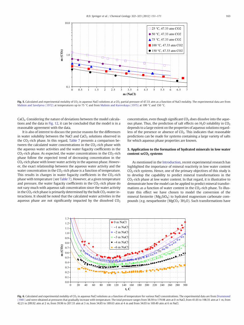
Fig. 4 shows the solubility in molality units of CO2 in aqueous NaClsolutions as a function of salt molality at 1 atm CO2 and temperaturesranging from 0 °C to 50 °C. Fig. 5 illustrates the CO2 solubility in thesame system at a pressure of 47.33 atm and temperatures rangingfrom 25 °C to 150 °C. At all temperatures, the solubility decreaseswith NaCl concentration following a classical salting-out patternwith a slow attenuation of the slope of the solubility vs. salt concen-tration curve as the concentration of NaCl increases. Fig. 6 showsthe temperature dependence of CO2 solubility over a wide range oftemperatures (0 to 300 °C) and NaCl molalities (0 to 6 molal). Itshould be noted that Fig. 6 does not represent solubility isobarsbecause the data of Drummond (1981) were obtained at pressuresthat gradually increase with temperature. Thus, the lines in Fig. 6only link the calculated results at pressures that correspond to the ex-perimental data at each temperature and do not constitute a ther-modynamic projection. As shown in Fig. 6, the experimental data(Drummond, 1981) show more scattering than those in Figs. 4–5.

Table 6Water solubility of saturated NaCl and CaCl2 solutions in scCO2 at 90 atm and differenttemperatures determined by NIR absorption spectroscopic measurements.

Temp. °C NaCl molality CaCl2 molality H2O Mol%

40 0 0 0.3240 Sat. NaCl 0 0.2240 Sat NaCl+3.0 g solid 0 0.2540 0 Sat. CaCl2 0.1640 0 Sat CaCl2+ 2.16 g solid 0.0550 0 0 0.4950 2 0 0.4850 4 0 0.4750 6 0 0.3850 Sat. NaCl 0 0.4050 Sat NaCl+3.0 g solid 0 0.4250 0 0.85 0.4450 0 2.94 0.3150 0 5.62 0.2050 0 Sat. CaCl2 0.1750 0 Sat CaCl2+ 2.16 g solid 0.1175 0 0 0.8575 Sat. NaCl 0 0.8875 Sat NaCl+3.0 g solid 0 0.8975 0 Sat. CaCl2 0.6275 0 Sat CaCl2+ 2.16 g solid 0.20100 0 0 1.61100 Sat. NaCl 0 1.68100 Sat NaCl+3.0 g solid 0 1.60100 0 Sat. CaCl2 1.12100 0 Sat CaCl2+ 2.16 g solid 0.46

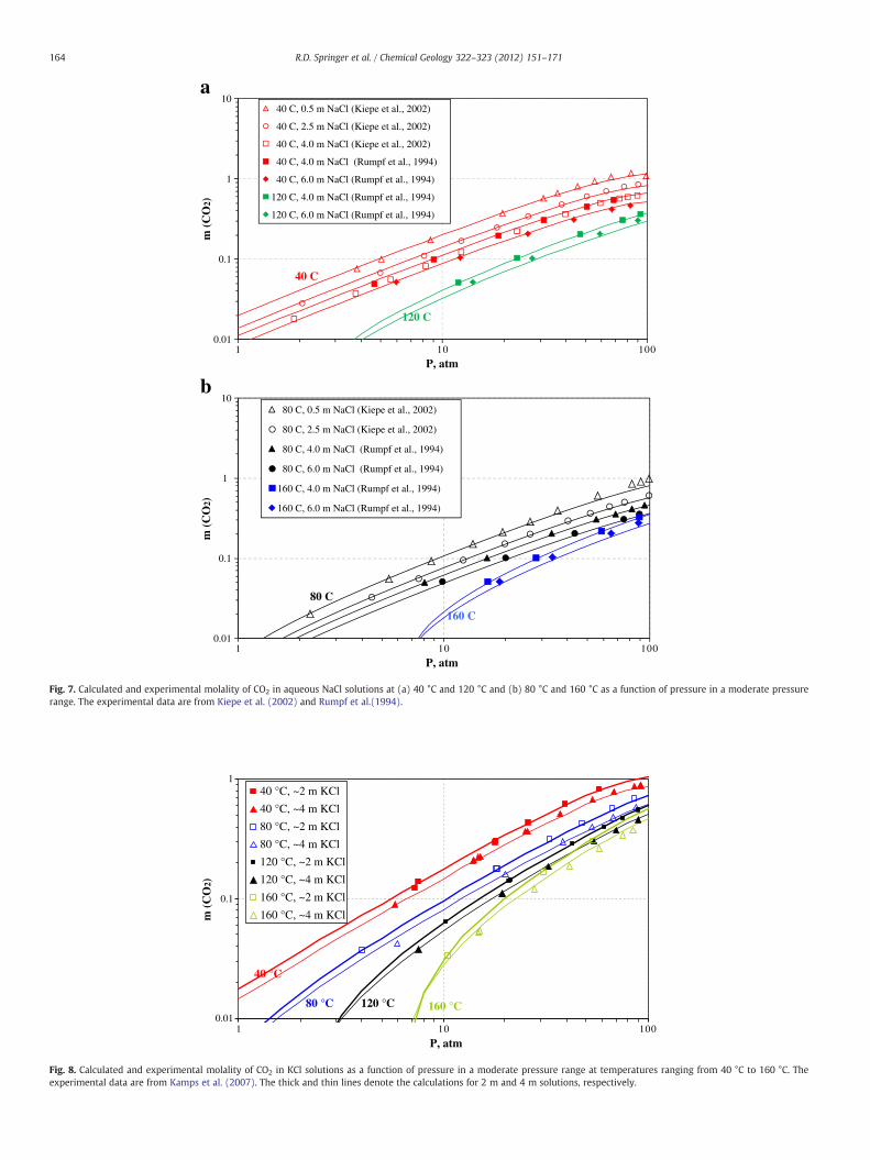
Nevertheless the calculated temperature trends are consistent withthe data. Fig. 7 shows the pressure dependence of CO2 solubilities inNaCl solutions at temperatures ranging from 40 °C to 160 °C and saltmolalities from 0.52 m to 6 m. For clarity, this figure is subdividedinto two diagrams (7a and 7b) to avoid the overlapping of solubilitycurves at various conditions. In the pressure range from 1 to 100 atm,the phase behavior is in the VLE-like range and, therefore, the CO2 sol-ubility increases with pressure with a relatively constant slope. Theslope decreases as the pressure approaches ~100 atm, reflecting a tran-sition to an LLE-like region. As shown in Figs. 4–7, the model accuratelyreproduces the dependence of CO2 solubility on temperature, pressure,andNaCl concentration inwide ranges of these variables,which encom-pass and go substantially beyond the conditions of CO2 sequestration.

The behavior of CO2 in KCl solutions is similar to that in NaCl solu-tions. This is illustrated in Fig. 8, which compares the calculationswith experimental data for temperatures up to 160 °C, pressures upto 100 atm and KCl concentrations up to 4 molal.

0.1

1

10

0.00001 0.0001 0.001 0.01 0.1xCO2

P /

a

Fig. 1. Calculated and experimental solubility of CO2 in H2O at 0, 25, 50, 100, and150 °C. The experimental data are from Prytz and Holst (1895), Findlay and Creighton(1910), Findlay and Shen (1912), Findlay and Williams (1913), Findlay and Howell(1915), Morgan and Pyne (1930), Morgan and Maass (1931), Kobe and Williams(1935), Shedlovsky and MacInnes (1935), Zelvenskii (1937), Wiebe and Gaddy(1939, 1940, 1941), Markham and Kobe (1941), Harned and Davis (1943), Dodds etal. (1956), Houghton et al. (1957), Novak et al. (1961), Tödheide and Franck (1963),Takenouchi and Kennedy (1964, 1965), Yeh and Peterson (1964), Vilcu and Gainar(1967), Matous et al. (1969), Stewart and Munjal (1970), Hayduk and Malik (1971),Murray and Riley (1971), Malinin and Savelyeva (1972), Malinin and Kurovskaya(1975), Drummond (1981), Shagiakhmetov and Tarzimanov (1981), Won et al.(1981), Zawisza and Malesińska (1981), Gillespie et al. (1984), Briones et al. (1987),Nakayama et al. (1987), Postigo and Katz (1987), DiSouza et al. (1988), Müller et al.(1988), Oyevaar et al. (1989), Carroll et al. (1991), King et al. (1992), Mather andFranck (1992), Dohrn et al. (1993), Rumpf et al. (1994), Bamberger et al. (2000),Kiepe et al. (2002), Bando et al. (2003), Chapoy et al. (2004), Valtz et al. (2004).

1

10

100

1000

10000

0.0001 0.001 0.01 0.1 1

P /

atm

King et al. (1992), 15 C

Valtz et al. (2004), 15.1 C

Gillespie et al. (1984), 15.6 C

King et al. (1992), 25 C

Valtz et al. (2004), 25.1 C

Gillespie et al. (1984), 25 C

Wiebe and Gaddy (1940, 1941), 25 C

Coan and King (1971), 25 C

Nakayama et al. (1987), 25 C

King et al. (1992), 40 C

Traub and Stephan (1990), 40 C

This work, 40 C

15 °C

25 °C

40 °C

a

1

10

100

1000

10000

0.001 0.01 0.1 1

P /

atm

Coan and King (1971), 50 CWiebe and Gaddy (1939), 50 CTodheide and Franck (1963), 50 CBriones et al. (1987), 50 CDiSouza et al. (1988), 50 CDohrn et al. (1993), 50 CBamberger et al. (2000), 50 CThis work, 50 CGillespie et al. (1984), 75 CCoan and King (1971), 75 CWiebe and Gaddy (1939), 75 CDiSouza et al. (1988), 75 CSako et al. (1991), 75 CThis work, 75 C

50 °C

75 °C

b

xH2O

xH2O

Fig. 2. Calculated and experimental solubility of H2O in CO2 at (a) 15, 25, and 40 °C and (b) 50 and 75 °C.


Measurements of CO2 solubilities in CaCl2 solutions are availableover wider ranges of salt concentration than in NaCl and KCl solu-tions. Fig. 9 shows the calculated and experimental CO2 solubilitiesat 47.33 atm CO2 and temperatures from 25 °C to 150 °C. Thus,Fig. 9 is analogous to Fig. 5 for NaCl solutions. The decrease in CO2 sol-ubility as a function of CaCl2 concentration is substantially strongerthan in NaCl solutions when the CO2 solubility is plotted as a functionof salt molality. Fig. 10 illustrates the effect of pressure on the solubil-ity of CO2 in CaCl2 solutions at temperatures ranging from 75 °C to120 °C and pressures up to 1000 atm. For clarity, Fig. 10 is subdividedinto two diagrams for CaCl2 concentrations of 1, 3.9, and 2.3 molal. Asshown in Fig. 10, the CO2 solubility transitions from a VLE-like regionwith a higher slope of CO2 molality vs. pressure to an LLE-like regionwith a lower slope. The model accurately represents the solubilitiesincluding the change in slope.

As illustrated by Figs. 4–10, the model provides an accurate repre-sentation of experimental data for water-rich phases in CO2–water–chloride salt systems. With the parameters determined on the basisof such data, it is then applied to predict the properties of CO2-richphases.

4.2.3. Prediction of water solubility in CO2‐rich phasesFigs. 11 and 12 compare the model predictions with the new ex-

perimental data for water solubility in CO2-rich phases. These figuresshow the solubility of H2O in the CO2-rich phase as a function of saltmolality in the coexisting H2O-rich phase. Fig. 11 presents the results

for the CO2–H2O–NaCl system. On an overall basis, the effect of NaClconcentration on the water solubility is small. As we will discussbelow, this results from the relatively small change in water activitythat occurs in NaCl solutions even at high concentration. At 40 °C,the model predictions match the data almost exactly. At 50 °C, thecalculated solubilities are offset by a constant amount relative to thedata. This offset is due to the small difference between the model cal-culations and the new data for salt-free systems, as illustrated inFig. 2b. This offset remains constant as a function of NaCl molality,thus indicating that the predicted effect of NaCl is the same as that in-dicated by the data. At 75 °C, the model is in an exact agreement withthe data in a NaCl-free system and somewhat underestimates the sol-ubility in the presence of concentrated NaCl solutions. At 100 °C, themodel predicts a slightly higher H2O solubility in a salt-free systemand is in a good agreement with the data in the presence of concen-trated NaCl. Thus, in view of the nature of the deviations, it can beconcluded that the model predictions are consistent with the newmeasurements.

In contrast to NaCl, CaCl2 has a substantial effect on the H2O solubil-ity in CO2 owing to the much lower water activity in CaCl2 solutions. Asshown in Fig. 12, the H2O solubility significantly decreases with CaCl2concentration. At 40 °C and 50 °C, the model is in a good agreementwith the data except for one solubility point for 11.7 molal CaCl2. At75 °C, the model underpredicts the data for 7.2 molal CaCl2 whereasthe agreement is reasonably good for 12.4 molal CaCl2. At 100 °C, themodel slightly underpredicts the solubilities for 7.2 and 13.6 molal

1

10

100

1000

10000

P /

atm

Coan and King (1971), 100 C

Todheide and Franck (1963), 100 C

Drummond (1981), 100 C

Muller et al. (1988), 100 C

This work, 100 C


Takenouchi and Kennedy (1964), 110 C

100 °C

110 °C

a

1

10

100

1000

10000

10.10.01

10.10.01

P /

atm


Muller et al. (1988), 120 C

Todheide and Franck (1963), 150 C



Takenouchi and Kennedy (1964), 150 C

120 °C

150 °C

b

xH2O

xH2O

Fig. 3. Calculated and experimental solubility of H2O in CO2 at (a) 100 and 110 °C and (b) 120 and 150 °C.

0.00

0.01

0.10

0 0.5 1 21.5 2.5 3 3.5 4 4.5 5 65.5 6.5

m (NaCl)

m (

CO

2)

0 °C, 1 atm CO2

15 °C, 1 atm CO2

25 °C, 1 atm CO2

35 °C, 1 atm CO2

50 °C, 1 atm CO2

Fig. 4. Calculated and experimental molality of CO2 in aqueous NaCl solutions at a CO2 partial pressure of 1 atm as a function of NaCl molality. The experimental data are fromBurmakina et al. (1982), Gerecke (1969), Harned and Davis (1943), He and Morse (1993), Kobe and Williams (1935), Mackenzie (1877), Markham and Kobe (1941), Onda et al.(1970a, 1970b), Setchenow (1892), Vazquez et al. (1994a, 1994b), Yasunishi and Yoshida (1979), and Yeh and Peterson (1964).


0.1

1.0

10.0

0 0.5 1 1.5 2 2.5 3 3.5 4 4.5 5 5.5 6 6.5 7

m (NaCl)

25 °C, 47.33 atm CO2

50 °C, 47.33 atm CO2

75 °C, 47.33 atm CO2

100 °C, 47.33 atm CO2

150 °C, 47.33 atm CO2

m (

CO

2)

Fig. 5. Calculated and experimental molality of CO2 in aqueous NaCl solutions at a CO2 partial pressure of 47.33 atm as a function of NaCl molality. The experimental data are fromMalinin and Savelyeva (1972) at temperatures up to 75 °C and from Malinin and Kurovskaya (1975) at 100 °C and 150 °C.


CaCl2. Considering the nature of deviations between the model calcula-tions and the data in Fig. 12, it can be concluded that the model is in areasonable agreement with the data.

It is also of interest to discuss the precise reasons for the differencesin water solubility between the NaCl and CaCl2 solutions observed inthe CO2-rich phase. In this regard, Table 7 presents a comparison be-tween the calculated water concentrations in the CO2-rich phase withthe aqueous water activities and the water fugacity coefficients in theCO2-rich phase. As expected, the water concentrations in the CO2-richphase follow the expected trend of decreasing concentration in theCO2-rich phase with lower water activity in the aqueous phase. Howev-er, the exact relationship between the aqueous water activity and thewater concentration in the CO2-rich phase is a function of temperature.This results in changes in water fugacity coefficients in the CO2-richphase with temperature (see Table 7). However, at a given temperatureand pressure, the water fugacity coefficients in the CO2-rich phase donot vary muchwith aqueous salt concentration since the water activityin the CO2-rich phase is primarily determined by the bulk CO2-water in-teractions. It should be noted that the calculated water activities in theaqueous phase are not significantly impacted by the dissolved CO2

0.0

0.1

0.2

0.3

0.4

0.5

0.6

0.7

0.8

0.9

1.0

1.1

1.2

1.3

0 20 40 60 80 100 120 140

t

0 m NaCl

~1 m NaC

~2 m NaC

~3 m NaC

~4 m NaC

~6 m NaC

m (

CO

2)

Fig. 6. Calculated and experimental molality of CO2 in aqueous NaCl solutions as a function of(1981) and were obtained at pressures that gradually increase with temperature. The total pres42.21 to 209.92 atm at 2 m, from 39.96 to 207.33 atm at 3 m, from 34.85 to 189.63 atm at 4 m

concentration, even though significant CO2 does dissolve into the aque-ous phase. Thus, the prediction of salt effects on H2O solubility in CO2

depends to a large extent on the properties of aqueous solutions regard-less of the presence or absence of CO2. This indicates that reasonablepredictions can be made for systems containing a large variety of saltsfor which aqueous phase properties are known.

5. Application to the formation of hydrated minerals in low watercontent scCO2 systems

As mentioned in the Introduction, recent experimental research hashighlighted the importance of mineral reactivity in low water contentCO2-rich systems. Hence, one of the primary objectives of this study isto develop the capability to predict mineral transformations in theCO2-rich phase at low water content. In that regard, it is illustrative todemonstrate how themodel can be applied to predict mineral transfor-mations as a function of water content in the CO2-rich phase. To illus-trate this effect we have chosen to model the conversion of themineral forsterite (Mg2SiO4) to hydrated magnesium carbonate com-pounds (e.g. nesquehonite (MgCO3·3H2O). Such transformations have

160 180 200 220 240 260 280 300

, C

l

l

l

l

l

temperature for various NaCl concentrations. The experimental data are from Drummondsure ranges from 38.59 to 179.98 atm at 0 mNaCl, from 41.65 to 198.35 atm at 1 m, fromand from 34.03 to 169.49 atm at 6 m NaCl.

0.01

0.1

1

10

001011

P, atm

40 C, 0.5 m NaCl (Kiepe et al., 2002)



40 C, 4.0 m NaCl (Rumpf et al., 1994)




40 C

120 C

a

0.01

0.1

1

10

001011

P, atm







b

80 C

160 C

m (

CO

2)m

(C

O2)

Fig. 7. Calculated and experimental molality of CO2 in aqueous NaCl solutions at (a) 40 °C and 120 °C and (b) 80 °C and 160 °C as a function of pressure in a moderate pressurerange. The experimental data are from Kiepe et al. (2002) and Rumpf et al.(1994).

0.01

0.1

1

001011

P, atm

40 °C, ~2 m KCl

40 °C, ~4 m KCl

80 °C, ~2 m KCl

80 °C, ~4 m KCl

120 °C, ~2 m KCl

120 °C, ~4 m KCl

160 °C, ~2 m KCl

160 °C, ~4 m KCl

40 °C

160 °C120 °C80 °C

m (

CO

2)

Fig. 8. Calculated and experimental molality of CO2 in KCl solutions as a function of pressure in a moderate pressure range at temperatures ranging from 40 °C to 160 °C. Theexperimental data are from Kamps et al. (2007). The thick and thin lines denote the calculations for 2 m and 4 m solutions, respectively.


0.0

0.1

1.0

10.0

0 1 2 3 4 5 6 7 8 9

m (CaCl2)

25 °C, 47.33 atm CO2

50 °C, 47.33 atm CO2

75 °C, 47.33 atm CO2

100 °C, 47.33 atm CO2

150 °C, 47.33 atm CO2

m (

CO

2)

Fig. 9. Calculated and experimental molality of CO2 in aqueous CaCl2 solutions at a CO2 partial pressure of 47.33 atm as a function of CaCl2 molality. The experimental data are fromMalinin and Savelyeva (1972) at 25 °C, 50 °C, and 75 °C and from Malinin and Kurovskaya (1975) at 100 °C and 150 °C.

0.01

0.1

1

10

000100101

P / atm

75 °C, 1 m CaCl2 75 °C, 3.9 m CaCl2

100 °C, 1 m CaCl2 100 °C, 3.9 m CaCl2

120 °C, 1 m CaCl2 120 °C, 3.9 m CaCl21 m CaCl2

3.9 m CaCl2

a

0.01

0.1

1

10

000100101

P / atm

75 °C, 2.3 m CaCl2

100 °C, 2.3 m CaCl2

120 °C, 2.3 m CaCl2

2.3 m CaCl2

b

m (

CO

2)m

(C

O2)

Fig. 10. Calculated and experimental molality of CO2 in aqueous CaCl2 solutions as a function of pressure at the temperatures of 75, 100, and 120 °C and CaCl2 concentrations of(a) 1 and 3.9 molal and (b) 2.3 molal. The experimental data are from Prutton and Savage (1945). The solubility isotherms at 75, 100, and 120 °C are denoted by the thin solid,thick solid, and dotted lines, respectively.


0.01

0.1

1

10

0 0.5 1 1.5 2 2.5 3 3.5 4 4.5 5 5.56 6.5 7

H2O

, mol

e %

m (NaCl)

40 C 50 C 75 C 100 C

H2Omin, 40°C

H2Omin, 100°C

H2Omin, 75°C

H2Omin, 50°C

Fig. 11. Comparison of model predictions with new experimental results obtained in this study for the solubility of water (in mole% units) in the CO2-rich phase in the NaCl–CO2–H2Osystem as a function of NaCl molality in the H2O-rich phase at 90 atm. The symbols show the experimental data (Table 6). The solid lines show the H2O solubilities obtained from themodel. The near-horizontal dashed lines denote the minimum H2O mole percent that is required for the transformation of forsterite into nesquehonite.


previously been demonstrated to occur in lowwater content scCO2 sys-tems (Loring et al., 2011; Felmy et al., 2012). The overall transformationreaction in scCO2 is

Mg2SiO4 þ 2CO2 þ 6H2O→2MgCO3⋅3H2Oþ SiO2 amð Þ ð23Þ

In the above reaction the water is dissolved in scCO2. Hence, inorder to predict the transformation of forsterite to nesquehonite, anaccurate model is required for the water fugacity in scCO2 as well asthe other phases in the system. Table 8 shows the results of ourmodel calculations of the water concentration in scCO2 required toachieve phase equilibrium between forsterite and nesquehonite atthe solution compositions measured in this study. The procedure formaking such calculations is outlined in the Appendix A. Also,Table 8 shows the calculated concentrations of H2O in the scCO2

phase, which correspond to the experimental measurements detailedin Table 6. The results show that at lower temperatures forsteriteshould transform to nesquehonite even at relatively low water satu-rations in scCO2. However, as the temperature increases, the waterconcentration required for nesquehonite to form also increases. In fact,this effect becomes so large that at temperatures greater than 75 °Cnesquehonite should not form at all from forsterite in H2O-saturated

0.01

0.1

1

10

0 1 2 3 4 5 6

H2O

, mol

e %

m (

H2Omin, 75°C

H2Omin, 40°CH2 Omin, 50°C

Fig. 12. Comparison of model predictions with new experimental results obtained in this studsystem as a function of CaCl2 molality in the H2O-rich phase at 90 atm. The symbols show themodel. The near-horizontal dashed lines denote the minimum H2O mole percent that is requi

scCO2 that is in contact with highly concentrated CaCl2 solutions sincethe required water saturation is greater than 100%.

6. Conclusions

Determining the chemical potential of variable concentrations ofH2O in supercritical CO2-rich phases has been approached using acombination of experimental measurements and thermodynamicmodeling. New measurements provide data on the solubility ofwater in the carbon dioxide-rich phase of ternary mixtures of CO2,H2O and NaCl or CaCl2. Thus, the new measurements fill a majorgap in the experimental database for CO2–water–salt systems, forwhich data have been previously available only for the H2O-richphase. At the same time, a comprehensive thermodynamic model hasbeen established for predicting the properties of CO2–H2O–chloridesalt systems in both the H2O-rich and CO2-rich phases. This modeltakes advantage of the large existing database for both phases in theCO2–H2O binary and the H2O-rich phase in the CO2–H2O–NaCl/KCl/CaCl2/MgCl2 ternary and multicompontent systems. The model, basedon the previously developed MSE framework for mixtures of elec-trolytes and nonelectrolytes over wide ranges of concentrations andtemperatures, represents the properties of these systems essentiallywithin the experimental scattering. Furthermore, the model predicts

7 8 9 10 11 12 13 14

CaCl2)

40 C 50 C 75 C 100 C

H2Omin, 100°C

y for the solubility of water (in mole% units) in the CO2-rich phase in the CaCl2–CO2–H2Oexperimental data (Table 6). The solid lines show the H2O solubilities obtained from the

red for the transformation of forsterite into nesquehonite (cf. Table 8).

Table 7Calculated water concentrations, activities and activity/fugacity coefficients in the CO2-rich phase as a function of temperature and salt concentrations.

Temp.°C

NaClmolality

CaCl2molality

CO2

molalityAqueous H2Oactivity

H2O mole fraction inCO2-rich phase

H2O fugacity coefficientin CO2-rich phase

CO2 fugacity coefficientin CO2-rich phase

H2O Activity inabsence of CO2

40 0 0 1.2357 0.9776 0.003538 0.2373 0.6275 140 6.14 0 0.4991 0.7437 0.002655 0.2408 0.6279 0.754840 6.22 0 0.4950 0.7403 0.002645 0.2405 0.6277 0.751240 0 7.2 0.2740 0.3155 0.001103 0.2461 0.6281 0.318240 0 10.1 0.1946 0.1941 0.000673 0.2483 0.6285 0.195750 0 0 1.1046 0.9802 0.003789 0.3700 0.6744 150 2 0 0.7722 0.9133 0.003526 0.3706 0.6744 0.930450 4 0 0.5739 0.8359 0.003221 0.3713 0.6744 0.849250 6 0 0.4517 0.7516 0.002889 0.3725 0.6747 0.761750 6.14 0 0.4451 0.7456 0.002866 0.3724 0.6746 0.755550 6.27 0 0.4392 0.7401 0.002845 0.3723 0.6746 0.749750 0 0.85 0.7768 0.9395 0.003628 0.3706 0.6745 0.957250 0 2.94 0.4095 0.7523 0.002890 0.3730 0.6749 0.761650 0 5.62 0.2739 0.4540 0.001732 0.3760 0.6753 0.457450 0 7.2 0.2362 0.3310 0.001259 0.3771 0.6754 0.333550 0 11.7 0.1420 0.1654 0.000627 0.3787 0.6755 0.166375 0 0 0.8683 0.9847 0.008499 0.5122 0.7545 175 6.14 0 0.3495 0.7513 0.006452 0.5147 0.7544 0.759075 6.46 0 0.3383 0.7378 0.006334 0.5148 0.7543 0.745275 0 7.2 0.1730 0.3699 0.003151 0.5201 0.7549 0.371975 0 12.4 0.1035 0.1809 0.001536 0.5240 0.7558 0.1816100 0 0 0.7459 0.9869 0.018909 0.5961 0.8111 1100 6.14 0 0.2983 0.7580 0.014409 0.6004 0.8109 0.7647100 6.68 0 0.2821 0.7361 0.013986 0.6011 0.8110 0.7422100 0 7.2 0.1396 0.4085 0.007694 0.6092 0.8117 0.4103100 0 13.6 0.0812 0.1859 0.003485 0.6157 0.8128 0.1864


the solubility of H2O in CO2-rich phases in agreement with the newmeasurements for the CO2–H2O–NaCl and CO2–H2O–CaCl2 systems.Considering the fact that, in the foreseeable future, experimental datafor CO2-rich phases in equilibriumwith salt-containingH2O-rich phasesare likely to be scarce, themodel can be usedwith confidence to predictthe effect of various salts on the concentration and activity of H2O in

Table 8The water mole fraction in the CO2-rich phase required for equilibrium betweenforsterite and nesquehonite (rxn 23) as a function of temperature and aqueous saltconcentration at 90 atm scCO2 pressure. Details on the calculations of water concentra-tions are given in the Appendix A.

Temp.°C

NaClmolality

CaCl2molality

H2O molefraction atsaturation

H2O molefractionrequired forreaction

% watersaturationrequired forreaction

40 0 0 0.003538 0.0002288 640 6.14 0 0.002655 0.0002257 840 6.22 0 0.002645 0.0002258 940 0 7.2 0.001103 0.0002208 2040 0 10.1 0.000673 0.0002191 3350 0 0 0.003789 0.0003419 950 2 0 0.003526 0.0003413 1050 4 0 0.003221 0.0003407 1150 6 0 0.002889 0.0003399 1250 6.14 0 0.002866 0.0003399 1250 6.27 0 0.002845 0.0003399 1250 0 0.85 0.003628 0.0003414 950 0 2.94 0.002890 0.0003397 1250 0 5.62 0.001732 0.0003373 1950 0 7.2 0.001259 0.0003364 2750 0 11.7 0.000627 0.0003351 5375 0 0 0.008499 0.001669 2075 6.14 0 0.006452 0.001659 2675 6.46 0 0.006334 0.001658 2675 0 7.2 0.003151 0.001645 5275 0 12.4 0.001536 0.001641 102100 0 0 0.018909 0.007455 39100 6.14 0 0.014409 0.007384 51100 6.68 0 0.013986 0.007382 53100 0 7.2 0.007694 0.007314 95100 0 13.6 0.003485 0.007286 209

CO2-rich phases. Since H2O activity in CO2-rich phases plays a key rolein mineral reactivity in CO2 sequestration environments and the MSEmodel combines phase and chemical equilibria in a uniform formalism,the model is expected to provide a useful tool for predicting mineraltransformations in supercritical CO2.

Acknowledgment

This work was supported by the U. S. Department of Energy(DOE), Office of Basic Energy Sciences through a Single InvestigatorSmall Group Research (SISGR) grant at Pacific Northwest NationalLaboratory (PNNL). The experimental work was performed at EMSL,the Environmental Molecular Sciences Laboratory, a national scientif-ic user facility sponsored by the Department of Energy's DOE Office ofBiological and Environmental Research, and located at PNNL. PNNL isoperated for DOE by Battelle Memorial Institute under Contract #DE-AC06-76RLO-1830.

Appendix A. A shortcut procedure for calculating the necessarywater content for mineral conversion

The equilibrium condition for the mineral conversion reaction(Eq. (23)) can be calculated from the standard thermodynamic rela-tionship

ln K ¼ − 1RT

∑iνiΔG

0fi ¼ ln∏

if νii ðA1Þ

When applied to Eq. (23), the equilibrium relationship becomes

ln K ¼ − 1RT ð2ΔG0

f MgCO3⋅3H2O sð Þ� �

þ ΔG0f SiO2 sð Þ� �

−ΔG0f Mg2SiO4 sð Þ� �

−2ΔG0f CO2 gð Þ� �

−6ΔG0f H2O gð Þ� �Þ

ðA2Þ


and

K ¼ 1f 2CO2

f 6H2O

¼ 1

PxCO2ϕCO2

� �2PxH2O

ϕH2O

� �6 ðA3Þ

In Eq. (A2), the standard Gibbs energies of formation for solidMgCO3∙3H2O, Mg2SiO4 and SiO2(am) and ideal-gas CO2 and H2O arecalculated using the thermochemical data that are summarized inTable 4. The fugacity coefficients in Eq. (A3) are obtained from themodel described in this study. As shown in Table 7, the fugacity coef-ficients of CO2 and H2O in the CO2-rich phase are very weak functionsof composition at a given temperature and pressure. Therefore, it canbe assumed that they remain practically constant within a reasonablerange of water contents. Further, it can be assumed that there is noappreciable dissolution of the minerals in the CO2-rich phase thatwould affect the fugacity coefficients. With these assumptions, thewater mole fraction that is necessary for the transformation offorsterite into nesquehonite can be calculated as

xH2O¼ 1

PϕH2Oexp −1

6ln K þ 2 ln f CO2

� �� ðA4Þ

The fugacity coefficients that are necessary to apply Eq. (A4) arelisted in Table 7 at the conditions of the experiments reported in thisstudy.

References

Abrams, D.S., Prausnitz, J.M., 1975. Statistical thermodynamics of liquid mixtures–newexpressions for excess Gibbs energy of partly or completely miscible systems.AICHE Journal 21, 116–128.

Akinfiev, N.N., Diamond, L.W., 2010. Thermodynamic model of aqueous CO2-H2O-NaClsolutions from −22 to 100 C and from 0.1 to 100 MPa. Fluid Phase Equilibria 295,104–124.

Anderko, A., Malanowski, S., 1992. Modeling Phase Equilibria: Thermodynamic Back-ground and Practical Tools. J. Wiley & Sons, New York, NY.

Anderko, A., Pitzer, K.S., 1993. Equation of state representation of phase equilibria andvolumetric properties of the systems NaCl-H2O above 573 K. Geochimica etCosmochimica Acta 57, 1657–1680.

Anderko, A., Wang, P., Rafal, M., 2002. Electrolyte solutions: from thermodynamic andtransport property models to the simulation of industrial processes. Fluid PhaseEquilibria 194, 123–142.

Angus, S., 1976. International Thermodynamic Tables of the Fluid State. Volume 3:Carbon Dioxide. Butterworths.

Austin, W.H., Lacombe, E., Rand, P.W., Chatterjee, M., 1963. Solubility of carbon dioxidein serum from 15 to 38 C. Journal of Applied Physiology 18, 301–304.

Bachu, S., 2002. Sequestration of CO2 in geological media in response to climatechange: road map for site selection using the transform of the geological spaceinto the CO2 phase space. Energy Conversion and Management 43, 87–102.

Bachu, S., 2008. CO2 storage in geological media: role, means, status and barriers todeployment. Progress in Energy and Combustion Science 34, 254–273.

Bachu, S., Adams, J.J., 2003. Sequestration of CO2 in geological media in response toclimate change: capacity of deep saline aquifers to sequester CO2 in solution.Energy Conversion and Management 44, 3151–3175.

Bamberger, A., Sieder, G., Maurer, G., 2000. High‐pressure (vapor + liquid) equilibriumin binary mixtures of (carbon dioxide +water or acetic acid) at temperatures from313 to 353 K. Journal of Supercritical Fluids 17, 97–110.

Bando, S., Takemura, F., Nishio, M., Hihara, E., Akai, M., 2003. Solubility of CO2 in aque-ous solutions of NaCl at (30 to 60) C and (10 to 20)MPa. Journal of Chemical andEngineering Data 48, 576–579.

Barta, L., Bradley, D.J., 1985. Extension of the specific interaction model to include gassolubilities in high-temperature brines. Geochimica et Cosmochimica Acta 49,195–203.

Bartels, H., Wrbitzky, R., 1960. Bestimmung des CO2 Absorptionskoeffizientenzwischen 15 und 38 C in Wasser und Plasma. Pflügers Archiv 271, 162–168.

Barton, J.R., Hsu, C.C., 1971. Solubility of cyclopropane in alkyl carboxylic acids. Journalof Chemical and Engineering Data 16, 93–95.

Benson, S.M., Surles, T., 2006. Carbon dioxide capture and storage: an overview withemphasis on capture and storage in deep geological formations. Proceedings ofthe IEEE 94, 1795–1805.

Blencoe, J.G., Naney, M.T., Anovitz, L.M., 2001. The CO2–H2O system: III. A new exper-imental method for determining liquid–vapor equilibria at high subcritical tem-peratures. American Mineralogist 86, 1100–1111.

Bohr, C., 1899. Definition und Methode zur Bestimmung der Invasions–undEvasionscoefficienten bei der Auflösung von Gasen in Flüssigkeiten. Werthe derGenannten Constanten Sowie der Absorptionscoefficienten der Kohlensäure bei

Auflösung in Wasser und in Chlornatriumlosungen. Annalen der Physik 304,500–525.

Bohr, C., Bock, J., 1891. Bestimmung der Absorption Einiger Gase in Wasser bei denTemperaturen zwischen 0 und 100 C. Annalen der Physik 280, 318–343.

Briones, J.A., Mullins, J.C., Thies, M.C., Kim, B.U., 1987. Ternary phase equilibria for aceticacid–water mixtures with supercritical carbon dioxide. Fluid Phase Equilibria 36,235–246.

Bunsen, R.W.E., 1855a. Memoire sur la loi de l'absorption des gaz par les liquides.Annales de Chimie et de Physique 43, 496–508.

Bunsen, R.W.E., 1855b. On the law of absorption of gases. Philosophical Magazine 9(116–130), 181–201.

Burmakina, G.V., Efanov, L.N., Shnet, M.A., 1982. Solubility of CO2 in aqueous solutionsof electrolytes and of sucrose. Russian Journal of Physical Chemistry 56, 705–707.

Carroll, J.J., Slupsky, J.D., Mather, A.E., 1991. The solubility of carbon dioxide in water atlow pressure. Journal of Physical and Chemical Reference Data 20, 1201–1209.

Chapoy, A., Mohammadi, A.H., Chareton, A., Tohidi, B., Richon, D., 2004. Measurementand modeling of gas solubility and literature review of the properties for the car-bon dioxide–water system. Industrial and Engineering Chemistry Research 43,1794–1802.

Coan, C.R., King, A.D.J., 1971. Solubility of water in compressed carbon dioxide, nitrousoxide, and ethane. Evidence for hydration of carbon dioxide and nitrous oxide inthe gas phase. Journal of the American Chemical Society 93, 1857–1862.

Cramer, S.D., 1982. The solubility of methane, carbon dioxide, and oxygen in brinesfrom 0 to 300 C: Bureau of Mines Report of Investigations, 8706.

Crovetto, R., 1991. Evaluation of solubility data of the system CO2-H2O from 273 K tothe critical point of water. Journal of Physical and Chemical Reference Data 20,575–589.

Crovetto, R., Wood, R.H., 1992. Solubility of CO2 in water and density of aqueous CO2

near the solvent critical temperature. Fluid Phase Equilibria 74, 271–288.Curry, J., Hazelton, C.L., 1938. The solubility of carbon dioxide in deuterium oxide at 25

C. Journal of the American Chemical Society 60, 2771–2773.Daval, D., Sissmann, O., Menguy, N., Saldi, G.D., Guyot, F., Martinez, I., Corvisier, J.,

Garcia, B., Machouk, I., Knauss, K.G., Hellmann, R., 2011. Influence of amorphoussilica layer formation on the dissolution rate of olivine at 90°C and elevatedpCO2. Chemical Geology 284, 193–209.

de Khanikof, N., Louguinine, V., 1867. Experiences pour verifier la loi de Henry etDalton sur l'absorption des gaz par les liquides a temperature constante et sousdes pressions variables. Annales de Chimie et de Physique 11, 412–433.

Dhima, A., de Hemptinne, J.C., Jose, J., 1999. Solubility of hydrocarbons and CO2 mix-tures in water under high pressure. Industrial and Engineering Chemistry Research38, 3144–3161.

Diamond, L.W., Akinfiev, N.N., 2003. Solubility of CO2 in water from −1.5 to 100 C andfrom 0.1 to 100 MPa: evaluation of literature data and thermodynamic modelling.Fluid Phase Equilibria 208, 265–290.

DiSouza, R., Patrick, J.R., Teja, A.S., 1988. High pressure phase equilibria in the carbondioxide — n-hexadecane and carbon dioxide–water systems. Canadian Journal ofChemical Engineering 66, 319–323.

Dodds, W.S., Stutzman, L.F., Sollami, B.J., 1956. Carbon dioxide solubility in water.Industrial and Engineering Chemistry Chemical and Engineering Data Series 1,92–95.

Dohrn, R., Bunz, A.P., Devlieghere, F., Thelen, D., 1993. Experimental measurements ofphase equilibria for ternary and quaternary systems of glucose, water, CO2 and eth-anol with a novel apparatus. Fluid Phase Equilibria 83, 149–158.

Drummond, J., S. E., 1981. Boiling and mixing of hydrothermal fluids: Chemical effectson mineral precipitation, PhD thesis, Pennsylvania State University.

Duan, Z.H., Sun, R., 2003. An improved model calculating CO2 solubility in pure waterand aqueous NaCl solutions from 273 to 533 K and from 0 to 2000 bar. ChemicalGeology 193, 257–271.

Duan, Z.H., Moller, N., Weare, J.H., 1995. Equation of state for the NaCl-H2O-CO2 system— prediction of phase-equilibria and volumetric properties. Geochimica etCosmochimica Acta 59, 2869–2882.

Duan, Z.H., Moller, N., Weare, J.H., 2003. Equations of state for the NaCl-H2O-CH4 sys-tem and the NaCl-H2O-CO2-CH4 system: phase equilibria and volumetric proper-ties above 573 K. Geochimica et Cosmochimica Acta 67, 671–680.

Duan, Z.H., Sun, R., Zhu, C., Chou, I.M., 2006. An improved model for the calculation ofCO2 solubility in aqueous solutions containing Na+, K+, Ca2+, Mg2+, Cl−, andSO4

2−. Marine Chemistry 98, 131–139.Ellis, A.J., 1959. The solubility of carbon dioxide in water at high temperatures. American

Journal of Science 257, 217–234.Ellis, A.J., Golding, R.M., 1963. The solubility of carbon dioxide above 100 C in water and

in sodium chloride solutions. American Journal of Science 261, 47–60.Eremina, A.O., Efanov, L.N., Sorokina, N.A., 1989. Structural transformation in aqueous

solutions of electrolytes. Russian Journal of Physical Chemistry 63, 1361–1363.Fan, S.S., Guo, T.M., 1999. Hydrate formation of CO2‐rich binary and quaternary gas

mixtures in aqueous sodium chloride solutions. Journal of Chemical and Engineer-ing Data 44, 829–832.

Felmy, A.R., Qafoku, O., Arey, B.W., Hu, J.Z., Hu, M., Schaef, H.T., Ilton, E.S., Hess, N.J.,Pearce, C.I., Feng, J., Rosso, K.M., 2012. Reaction of water-saturated super-criticalCO2 with forsterite: evidence for magnesite formation at low temperatures.Geochimica et Cosmochimica Acta 91, 271–282.

Fenghour, A., Wakeham, W.A., Watson, J.T.R., 1996. Densities of (water + carbon diox-ide) in the temperature range 415 K to 700 K and pressures up to 35 MPa. TheJournal of Chemical Thermodynamics 28, 433–446.

Findlay, A., Creighton, H.J.M., 1910. The influence of colloids and fine suspensions onthe solubility of gases in water. Part I. Solubility of carbon dioxide and nitrousoxide. Journal of the Chemical Society 97, 536–561.


Findlay, A., Howell, O.R., 1915. The solubility of carbon dioxide in water in the presenceof starch. Journal of the Chemical Society 107, 282–284.

Findlay, A., Shen, B., 1912. The influence of colloids and fine suspensions on the solubil-ity of gases in water. Part II. Solubility of carbon dioxide and of hydrogen. Journal ofthe Chemical Society 101, 1459–1468.

Findlay, A., Williams, T., 1913. The influence of colloids and fine suspensions on the sol-ubility of gases in water. Part III. Solubility of carbon dioxide at pressures lowerthan atmospheric. Journal of the Chemical Society 103, 636–645.

Garcia, B., Beaumont, V., Perfetti, E., Rouchon, V., Blanchet, D., Oger, P., Dromart, G., Huc,A.Y., Haeseler, F., 2010. Experiments and geochemical modelling of CO2 sequestra-tion by olivine: potential, quantification. Applied Geochemistry 25, 1383–1396.

Garner, F.H., Long, R., Miller, D.G., 1959. Equilibria, at moderate pressures, in the systemCO2, H2S, N2 — sodium carbonate, sodium bicarbonate, sodium hydrosulfide andwater. Journal of Applied Chemistry 9, 534–542.

Geffcken, G., 1904. Articles on knowledge of solubility influencing. Zeitschrift furPhysikalische Chemie Stochiometrie und Verwandtschaftslehre 49, 257–302.

Gehrig, M., 1980. Phase equilibria and PVT data in the ternary mixture water, carbondioxide, and sodium chloride to 3 kbar and 550 C, PhD thesis, UniversityKarlsruhe.

Gerecke, J., 1969. Ein Beitrag zur Gaslöslichkeit in Elektrolytlösungen Untersucht amBeispiel der Löslichkeit von H2, CO2 und NH3 in Wasser und WässrigenSalzlösungen, PhD thesis, Technische Hochschule für Chemie Carl SchorlemmerLeuna Merseburg.

Giammar, D.E., Bruant, R.G., Peters, C.A., 2005. Forsterite dissolution and magnesiteprecipitation at conditions relevant for deep saline aquifer storage and sequestra-tion of carbon dioxide. Chemical Geology 217, 257–276.

Gillespie, P.C., Owens, J.L., Wilson, G.M., 1984. Sour Water Equilibria Extended to HighTemperatures and with Inerts Present. AIChE Winter National Meeting Atlanta,paper 34-b.

Gruszkiewicz, M.S., Palmer, D.A., Springer, R.D., Wang, P.M., Anderko, A., 2007. PhaseBehavior of aqueous Na-K-Mg-Ca-Cl-NO3 mixtures: Isopiestic measurements andthermodynamic modeling. Journal of Solution Chemistry 36, 723–765.

Gurvich, L.V., Veyts, I.V., Alcock, C.B., 1990. Thermodynamic properties of individualsubstances, 4th ed. Hemisphere Publishing Corporation.

Guyot, F., Daval, D., Dupraz, S., Martinez, I., Menez, B., Sissmann, O., 2011. CO2 geolog-ical storage: the environmental mineralogy perspective. Comptes Rendus Geosci-ence 343, 246–259.

Haar, L., Gallagher, J.S., Kell, G.S., 1984. NBS/NRC steam tables: thermodynamic andtransport properties and computer programs for vapor and liquid states in SIunits. Hemisphere Publishing, Washington, DC.

Hanchen, M., Prigiobbe, V., Storti, G., Seward, T.M., Mazzotti, M., 2006. Dissolutionkinetics of fosteritic olivine at 90–150°C including effects of the presence of CO2.Geochimica et Cosmochimica Acta 70, 4403–4416.

Hanchen, M., Prigiobbe, V., Baciocchi, R., Mazzotti, M., 2008. Precipitation in theMg-carbonate system — effects of temperature and CO2 pressure. ChemicalEngineering Science 63, 1012–1028.

Hantzsch, A., Vogt, A., 1901. On the state of soluble materials on the basis of spacing tests.Zeitschrift fur Physikalische Chemie Stochiometrie und Verwandtschaftslehre 38,705–742.

Harned, H.S., Davis Jr., R., 1943. The ionization constant of carbonic acid in water andthe solubility of carbon dioxide in water and aqueous salt solutions from 0 to 50C. Journal of the American Chemical Society 65, 2030–2037.

Harvey, A.H., Prausnitz, J.M., 1989. Thermodynamics of high-pressure aqueous systemscontaining gases and salts. AICHE Journal 35, 635–644.

Hayduk, W., Malik, V.K., 1971. Density, viscosity, and carbon dioxide solubility and dif-fusivity in aqueous ethylene glycol solutions. Journal of Chemical and EngineeringData 16, 143–146.

He, S.L., Morse, J.W., 1993. The carbonic acid system and calcite solubility in aqueousNa-K-Ca-Mg-Cl-SO4 solutions from 0 to 90 C. Geochimica et Cosmochimica Acta57, 3533–3554.

Helgeson, H.C., Kirkham, D.H., Flowers, G.C., 1974a. Theoretical prediction of the ther-modynamic behavior of aqueous electrolytes at high pressures and temperatures.I Summary of the thermodynamic/electrostatic properties of the solvent. AmericanJournal of Science 274, 1089–1198.

Helgeson, H.C., Kirkham, D.H., Flowers, G.C., 1974b. Theoretical prediction of the ther-modynamic behavior of aqueous electrolytes at high pressures and temperatures.II Debye–Hűckel parameters for activity coefficients and relative partial molalproperties. American Journal of Science 274, 1199–1261.

Helgeson, H.C., Kirkham, D.H., Flowers, G.C., 1976. Theoretical prediction of the ther-modynamic behavior of aqueous electrolytes at high pressures and temperatures.III Equation of state for aqueous species at infinite dilution. American Journal ofScience 276, 97–240.

Helgeson, H.C., Kirkham, D.H., Flowers, G.C., 1981. Theoretical prediction of the ther-modynamic behavior of aqueous electrolytes at high pressures and temperatures.IV. Calculation of activity coefficients, osmotic coefficients, and apparent molaland standard and relative partial molal properties to 5 kb and 600°C. AmericanJournal of Science 281.

Houghton, G., McLean, A.M., Ritchie, P.D., 1957. Compressibility, fugacity, and watersolubility of carbon dioxide in the region 0–36 atm and 0–100 C. Chemical Engi-neering Science 6, 132–137.

Jackson, K., Bowman, L.E., Fulton, J.L., 1995. Water solubility measurements in super-critical fluids and high‐pressure liquids using near‐infrared spectroscopy. Analyti-cal Chemistry 67, 2368–2372.

Ji, X.Y., Tan, S.P., Adidharma, H., Radosz, M., 2005. SAFT1-RPM approximation extendedto phase equilibria and densities of CO2-H2O and CO2-H2O-NaCl systems. Industrialand Engineering Chemistry Research 44, 8419–8427.

Jin, G., Donohue, M.D., 1988. An equation of state for electrolyte solutions. 2. Singlevolatile weak electrolytes in water. Industrial and Engineering Chemistry Research27, 1737–1743.

Johnson, J.W., Oelkers, E.H., Helgeson, H.C., 1992. SUPCRT92 — a software package forcalculating the standard molal thermodynamic properties of minerals, gases, aque-ous species, and reactions from 1 bar to 5000 bar and 0 °C to 1000 °C. Computers& Geosciences 18, 899–947.

Kamps, A.P.S., Meyer, E., Rumpf, B., Maurer, G., 2007. Solubility of CO2 in aqueous solu-tions of KCl and in aqueous solutions of K2CO3. Journal of Chemical and Engineer-ing Data 52, 817–832.

Kiepe, J., Horstmann, S., Fischer, K., Gmehling, J., 2002. Experimental determination andprediction of gas solubility data for CO2 + H2O mixtures containing NaCl or KCl attemperatures between 313 and 393 K and pressures up to 10 MPa. Industrial andEngineering Chemistry Research 41, 4393–4398.

King, M.B., Mubarak, A., Kim, J.D., Bott, T.R., 1992. The mutual solubilities of water withsupercritical and liquid carbon dioxide. Journal of Supercritical Fluids 5, 296–302.

King, H.E., Plumper, O., Putnis, A., 2010. Effect of secondary phase formation on the car-bonation of olivine. Environmental Science & Technology 44, 6503–6509.

Kobe, K.A., Williams, J.S., 1935. Confining liquids for gas analysis. Solubility of carbon diox-ide in salt solutions. Industrial and Engineering Chemistry, Analytical Edition 7, 37–38.

Koch Jr., H.A., Stutzman, L.F., Blum, H.A., Hutchings, L.E., 1949. Gas absorption. Liquidtransfer coefficients for the carbon dioxide–air–water system. Chemical Engineer-ing Progress 45, 677–682.

Koschel, D., Coxam, J.Y., Rodier, L., Majer, V., 2006. Enthalpy and solubility data of CO2

in water and NaCl(aq) at conditions of interest for geological sequestration. FluidPhase Equilibria 247, 107–120.

Kosinski, J.J., Wang, P.M., Springer, R.D., Anderko, A., 2007. Modeling acid-base equilib-ria and phase behavior in mixed-solvent electrolyte systerns. Fluid Phase Equilibria256, 34–41.

Kritschewski, I.R., Shaworonkoff, N.M., Aepelbaum, V.A., 1935. Combined solubility ofgases in liquids under pressure. I. Solubility of carbon dioxide in water from itsmixtures with hydrogen of 20 and 30 C and total pressure of 30 kg/cm2. Zeitschriftfür Physikalische Chemie Abteilung A 175, 232–238.

Kunerth, W., 1922. Solubility of CO2 and N2O in certain solvents. Physical Review 19,512–524.

Kwak, J.H., Hu, J.Z., Hoyt, D.W., Sears, J.A., Wang, C.M., Rosso, K.M., Felmy, A.R., 2010.Metal carbonation of forsterite in supercritical CO2 and H2O using solid state Si-29, C-13 NMR spectroscopy. Journal of Physical Chemistry C 114, 4126–4134.

Kwak, J.H., Hu, J.Z., Turcu, R.V.F., Rosso, K.M., Ilton, E.S., Wang, C., Sears, J.A., Engelhard,M.H., Felmy, A.R., Hoyt, D.W., 2011. The role of H2O in the carbonation of forsteritein supercritical CO2. International Journal of Greenhouse Gas Control 5,1081–1092.

Li, D., Duan, Z., 2007. The speciation equilibrium coupling with phase equilibrium inthe H2O-CO2-NaCl system from 0 to 250 C, from 0 to 1000 bar, and from 0 to 5molality of NaCl. Chemical Geology 244, 730–751.

Li, J., Duan, Z., 2011. A thermodynamic model for the prediction of phase equilibria andspeciation in the H2O-CO2-NaCl-CaCO3-CaSO4 system from 0 to 250 degrees C, 1 to1000 bar with NaCl concentrations up to halite saturation. Geochimica etCosmochimica Acta 75, 4351–4376.

Li, Y.K., Nghiem, L.X., 1986. Phase equilibria of oil, gas and water brine mixtures from acubic equation of state and Henry law. Canadian Journal of Chemical Engineering64, 486–496.

Li, Y.H., Tsui, T.F., 1971. Solubility of CO2 in water and sea water. Journal of GeophysicalResearch 76, 4203–4207.

Li, J.D., Topphoff, M., Fischer, K., Gmehling, J., 2001. Prediction of gas solubilities inaqueous electrolyte systems using the predictive Soave–Redlich–Kwong model.Industrial and Engineering Chemistry Research 40, 3703–3710.

Li, Z., Dong, M., Li, S., Dai, L., 2004. Densities and solubilities for binary systems of car-bon dioxide + water and carbon dioxide + brine at 59 C and pressures to 29 MPa.Journal of Chemical and Engineering Data 49, 1026–1031.

Lin, Y., Thomsen, K., de Hemptinne, J.C., 2007. Multicomponent equations of state forelectrolytes. AICHE Journal 53, 989–1005.

Lin, H., Fujii, T., Takisawa, R., Takahashi, T., Hashida, T., 2008. Experimental evaluationof interactions in supercritical CO2/water/rock minerals system under geologicCO2 sequestration conditions. Journal of Materials Science 43, 2307–2315.

Loring, J.S., Thompson, C.J., Wang, Z.M., Joly, A.G., Sklarew, D.S., Schaef, H.T., Ilton, E.S., Rosso,K.M., Felmy, A.R., 2011. In situ infrared spectroscopic study of forsterite carbonation inwet supercritical CO2. Environmental Science & Technology 45, 6204–6210.

Mackenzie, J.J., 1877. Űber die Absorption der Gase durch Salzlösungen. Annalen derPhysik 237, 438–451.

Mäder, U.K., 1991. H2O-CO2 mixtures — a review of P–V–T–X data and an assessmentfrom a phase equilibrium point of view. The Canadian Mineralogist 29, 767–790.

Malinin, S.D., 1959. The system water — carbon dioxide at high temperatures and pres-sures. Geochemistry 3, 292–306.

Malinin, S.D., Kurovskaya, N.A., 1975. Solubility of CO2 in chloride solutions at elevatedtemperatures and CO2 pressures. Geochemistry International 12, 199–201.

Malinin, S.D., Savelyeva, N.I., 1972. Experimental investigations of CO2 solubility inNaCl and CaCl2 solutions at temperatures of 25, 50 and 75 C and elevated CO2 pres-sure. Geochemistry International 9, 410–418.

Markham, A.E., Kobe, K.A., 1941. The solubility of carbon dioxide and nitrous oxide inaqueous salt solutions. Journal of the American Chemical Society 63, 449–454.

Mather, A.E., Franck, E.U., 1992. Phase equilibria in the system carbon dioxide–water atelevated pressures. Journal of Physical Chemistry 96, 6–8.

Matous, J., Sobr, J., Novak, J.P., Pick, J., 1969. Solubility of carbon dioxide in water atpressures up to 40 atm. Collection of Czechoslovak Chemical Communications34, 3982–3985.


McGrail, B.P., Schaef, H.T., Glezakou, V.A., Dang, L.X., Owen, A.T., 2009. Water reactivityin the liquid and supercritical CO2 phase: Has half the story been neglected? In:Gale, J., Herzog, H., Braitsch, J. (Eds.), Greenhouse Gas Control Technologies, p. 9.

Morgan, O.M., Maass, O., 1931. An investigation of the equilibria existing in gas–watersystems forming electrolytes. Canadian Journal of Research 5, 162–199.

Morgan, J.L.R., Pyne, H.R., 1930. Solubility relations in gas–liquid systems. I. A newapparatus for determining gas solubilities. Journal of Physical Chemistry 34,1578–1582.

Morrison, T.J., Billett, F., 1952. The salting‐out of non‐electrolytes. Part II. The effect ofvariation in non-electrolyte. Journal of the Chemical Society 3819–3822.

Müller, G., Bender, E., Maurer, G., 1988. Vapor liquid equilibrium in the ternary systemammonia–carbon dioxide–water at high water contents in the range 373 K to 473K. Berichte der Bunsengesellschaft für Physikalische Chemie 92, 148–160.

Murray, C.N., Riley, J.P., 1971. The solubility of gases in distilled water and sea water: IV.Carbon dioxide. Deep Sea Research 18, 533–541.

Nakayama, T., Sagara, H., Arai, K., Saito, S., 1987. High pressure liquid–liquid equilibriafor the system of water, ethanol and 1,1-difluoroethane at 323.2 K. Fluid PhaseEquilibria 38, 109–127.

Nighswander, J.A., Kalogerakis, N., Mehrotra, A.K., 1989. Solubilities of carbon dioxidein water and 1 wt% NaCl solution at pressures up to 10 MPa and temperaturesfrom 80 to 200 C. Journal of Chemical and Engineering Data 34, 355–360.

Nordbotten, J.M., Celia, M.A., 2006. Similarity solutions for fluid injection into confinedaquifers. Journal of Fluid Mechanics 561, 307–327.

Novak, J., Fried, V., Pick, J., 1961. Löslichkeit des Kohlendioxyds in Wasser beiVerschiedenen Drücken und Temperaturen. Collection of Czechoslovak ChemicalCommunications 26, 2266–2270.

Ohgaki, K., Makihara, Y., Takano, K., 1993. Formation of CO2 hydrate in pure and seawaters. Journal of Chemical Engineering of Japan 26, 558–564.

OLISystems, 2012. OLI Software: Stream Analyzer and ESP (Electrolyte Simulation Pro-gram), version 9.0.

Onda, K., Sada, E., Kobayashi, T., Kito, S., Ito, K., 1970a. Salting‐out parameters of gas sol-ubility in aqueous salt solutions. Journal of Chemical Engineering of Japan 3, 18–24.

Onda, K., Sada, E., Kobayashi, T., Kito, S., Ito, K., 1970b. Solubility of gases in aqueous so-lutions of mixed salts. Journal of Chemical Engineering of Japan 3, 137–142.

Oyevaar, M.H., Morssinkhof, R.W.J., Westerterp, K.R., 1989. Density, viscosity, solubility,and diffusivity of CO2 and N2O in solutions of diethanolamine in aqueous ethyleneglycol at 298 K. Journal of Chemical and Engineering Data 34, 77–82.

Pitzer, K.S., 1973. Thermodynamics of electrolytes. I. Theoretical basis and generalequations. Journal of Physical Chemistry 77, 268–277.

Pitzer, K.S., 1980. Electrolytes — from dilute solutions to fused salts. Journal of theAmerican Chemical Society 102, 2902–2906.

Pitzer, K.S., 1995. Thermodynamics, 3rd edition. McGraw-Hill, New York.Postigo, M.A., Katz, M., 1987. Solubility and thermodynamics of carbon dioxide in aque-

ous ethanol solutions. Journal of Solution Chemistry 16, 1015–1024.Power, G.G., Stegall, H., 1970. Solubility of gases in human red blood cell ghosts. Journal

of Applied Physiology 29, 145–149.Prigiobbe, V., Costa, G., Baciocchi, R., Hanchen, M., Mazzotti, M., 2009. The effect of CO2

and salinity on olivine dissolution kinetics at 120°C. Chemical Engineering Science64, 3510–3515.

Prutton, C.F., Savage, R.L., 1945. The solubility of carbon dioxide in calcium chloride–water solutions at 75, 100, 120 C and high pressures. Journal of the AmericanChemical Society 67, 1550–1554.

Prytz, K., Holst, H., 1895. Die Absorptionscoefficienten der Kohlensäure und desSchweffelwasserstoffs in Wasser bei dessen Gefrierpunkt. Annalen der Physik290, 130–139.

Rafal, M., Berthold, J.W., Scrivner, N.C., Grise, S.L., 1995. Models for Electrolyte Solu-tions. In: Sandler, S.I. (Ed.), Models for Thermodynamic and Phase Equilibria Calcu-lations. Marcel Dekker, New York.

Regnault, O., Lagneau, V., Catalette, H., Schneider, H., 2005. Experimental study of puremineral phases/supercritical CO2 reactivity. Implications for geological CO2 seques-tration. Comptes Rendus Geoscience 337, 1331–1339.

Robie, R.A., Hemingway, B.S., 1995. Thermodynamic properties of minerals and relatedsubstances at 298.15 K and 1 bar (105 Pa) pressure and at higher temperatures.U.S. Geological Survey Bulletin 2131, 461.

Rosenthal, W., 1954. Contribution a l'étude de la solubilité des gaz dans quelquessolvants et solutions, PhD thesis, University Strasbourg, France.

Rumpf, B., Nicolaisen, H., Ocal, C., Maurer, G., 1994. Solubility of carbon dioxide in aque-ous solutions of sodium chloride: experimental results and correlation. Journal ofSolution Chemistry 23, 431–448.

Sako, T., Sugeta, T., Nakazawa, N., Okubo, T., Sato, M., Taguchi, T., Hiaki, T., 1991. Phaseequilibrium study of extraction and concentration of furfural produced in reactorusing supercritical carbon dioxide. Journal of Chemical Engineering of Japan 24,449–455.

Salari, H., Hassanzadeh, H., Gerami, S., Abedi, J., 2011. On estimating the water contentof CO2 in equilibrium with formation brine. Petroleum Science and Technology 29,2037–2051.

Sander, W., 1912. On the solubility of carbon acid in water and some other solutionsunder high pressure. Zeitschrift für Physikalische Chemie Stochiometrie undVerwandtschaftslehre 78, 513–549.

Scharlin, P., 1996. Carbon dioxide in water and aqueous electrolyte solutions, IUPACSolubility Data Series 62. Pergamon Press.

Servio, P., Englezos, P., 2001. Effect of temperature and pressure on the solubility of car-bon dioxide in water in the presence of gas hydrate. Fluid Phase Equilibria 190,127–134.

Setchenow, J., 1879. Mémoires de l'Academie Imperiale des Sciences de Saint-Petersbourg 7th Series 26, 1–62.

Setchenow, J., 1887. Mémoires de l'Academie Imperiale des Sciences de Saint-Petersbourg 7th Series 35, 1–59.

Setchenow, J., 1889. Mosk. Obsh. Spyt. Prirody. Nouveaux Mémoires de la SociétéImpériale des Naturalistes de Moscou 15, 203–274.

Setchenow, J., 1892. Action de l'acide carbonique sur les solutions des sels a acidesforts. Etude absorptiometrique. Annales de Chimie et de Physique 25, 226–270.

Setschenow, S., 1874. Über die Absorptiometrie in Ihrer Anwendung auf die Zuständeder Kohlensäure im Blute. Pflügers Archiv 8, 1–39.

Shagiakhmetov, R.A., Tarzimanov, A.A., 1981. Measurements of CO2 solubility in waterup to 60 MPa. Deposited Document SPSTL 200khp D81, cited in Scharlin (1996).

Shchennikova, M.K., Devyatykh, G.G., Korshunov, I.A., 1957. Russian Journal of AppliedChemistry 30, 881–886.

Shedlovsky, T., MacInnes, D.A., 1935. The first ionization constant of carbonic acid, 0 to38 C, from conductance measurements. Journal of the American Chemical Society57, 1705–1710.

Shock, E.L., Helgeson, H.C., 1988. Calculation of the thermodynamic and transportproperties of aqueous species at high pressures and temperatures: Correlation al-gorithms for ionic species and equation of state predictions to 5 kb and 1000°C.Geochimica et Cosmochimica Acta 52, 2009–2036.

Shock, E.L., Helgeson, H.C., Sverjensky, D.A., 1989. Calculation of the thermodynamicand transport properties of species at high pressures and temperatures: Standardpartial molar properties of inorganic neutral species. Geochimica et CosmochimicaActa 53, 2157–2183.

Soave, G., 1972. Equilibrium constants from a modified Redlich-Kwong equation ofstate. Chemical Engineering Science 27, 1197-&.

Spycher, N., Pruess, K., 2005. CO2-H2O mixtures in the geological sequestration of CO2.II. Partitioning in chloride brines at 12-100 C and up to 600 bar. Geochimica etCosmochimica Acta 69, 3309–3320.

Spycher, N., Pruess, K., Ennis-King, J., 2003. CO2-H2O mixtures in the geological seques-tration of CO2. I. Assessment and calculation of mutual solubilities from 12 to 100 Cand up to 600 bar. Geochimica et Cosmochimica Acta 67, 3015–3031.

Sterner, S.M., Bodnar, R.J., 1991. Synthetic fluid inclusions. X: Experimental determina-tion of P–V–T–X properties in the CO2–H2O system to 6 kb and 700 C. AmericanJournal of Science 291, 1–54.

Stewart, P.B., Munjal, P., 1970. Solubility of carbon dioxide in pure water, synthetic seawater, and synthetic sea water concentrates at -5 to 25 C and 10 to 45 atm pres-sure. Journal of Chemical and Engineering Data 15, 67–71.

Stone, H.W., 1943. Solubility of water in liquid carbon dioxide. Industrial and Engineer-ing Chemistry 35, 1284–1286.

Suto, Y., Liu, L.H., Yamasaki, N., Hashida, T., 2007. Initial behavior of granite in responseto injection of CO2-saturated fluid. Applied Geochemistry 22, 202–218.

Takenouchi, S., Kennedy, G.C., 1964. The binary system H2O–CO2 at high temperaturesand pressures. American Journal of Science 262, 1055–1074.

Takenouchi, S., Kennedy, G.C., 1965. The solubility of carbon dioxide in NaCl solutionsat high temperatures and pressures. American Journal of Science 263, 445–454.

Tan, S.P., Adidharma, H., Radosz, M., 2008. Recent advances and applications of Statis-tical Associating Fluid Theory. Industrial and Engineering Chemistry Research 47,8063–8082.

Tanger, J.C., Helgeson, H.C., 1988. Calculation of the thermodynamic and transportproperties of aqueous species at high pressures and temperatures: revised equa-tions of state for the standard partial molal properties of ions and electrolytes.American Journal of Science 288, 19–98.

Teng, H., Yamasaki, A., Chun, M.K., Lee, H., 1997. Solubility of liquid CO2 in water attemperatures from 278 K to 293 K and pressures from 6.44 MPa to 29.49 MPaand densities of the corresponding aqueous solutions. The Journal of ChemicalThermodynamics 29, 1301–1310.

Tödheide, K., Franck, E.U., 1963. Das Zweiphasengebeit und die Kritische Kurve imSystem Kohlendioxid - Wasser bis zu Drucken von 3500 bar. Zeitschrift furPhysikalische Chemie Frankfurt 37, 387–401.

Traub, P., Stephan,K., 1990.High‐pressurephase equilibria of the systemCO2–water–acetonemeasured with a new apparatus. Chemical Engineering Science 45, 751–758.

TRC, 1989. TRC Thermodynamics Tables — Non-hydrocarbons. ThermodynamicResearch Center, The Texas A & M University System, College Station, TX.

Valtz, A., Chapoy, A., Coquelet, C., Paricaud, P., Richon, D., 2004. Vapor–liquid equilibriain the carbon dioxide–water system, measurement and modeling from 278.2 to318.2 K. Fluid Phase Equilibria 226, 333–344.

Van Slyke, D.D., 1939. Determination of solubilities of gases in liquids with use of theVan Slyke–Neill manometric apparatus for both saturation and analysis. Journalof Biological Chemistry 130, 545–554.

Vazquez, G., Chenlo, F., Pereira, G., 1994a. CO2 diffusivity in NaCl and CuSO4 aqueoussolutions. Afinidad 51, 369–374.

Vazquez, G., Chenlo, F., Pereira, G., Peaguda, J., 1994b. Solubility of CO2 in aqueous so-lutions of NaCl, CuSO4, KI and NaBr. Anales de Quimica 90, 324–328.

Vilcu, R., Gainar, I., 1967. Löslichkeit der Gase unter Druck in Flüssigkeiten I. Das SystemKohlendioxid - Wasser. Revue Roumaine de Chimie 12, 181–189.

Wagman, D.D., Evans, W.H., Parker, V.B., Schumm, R.H., Halow, I., Bailey, S., Churney,K.L., Nuttal, R.L., 1982. The NBS tables of chemical thermodynamic properties. Se-lected values for inorganic and C1 and C2 organic substances in SI units, Supple-ment 2. Journal of Physical and Chemical Reference Data 11, 2–392.

Wang, P.M., Anderko, A., Young, R.D., 2002. A speciation-based model for mixed-solvent electrolyte systems. Fluid Phase Equilibria 203, 141–176.

Wang, P., Springer, R.D., Anderko, A., Young, R.D., 2004. Modeling phase equilibria andspeciation in mixed-solvent electrolyte systems. Fluid Phase Equilibria 222, 11–17.

Wang, P., Anderko, A., Springer, R.D., Young, R.D., 2006. Modeling phase equilibria and spe-ciation inmixed-solvent electrolyte systems: II. Liquid–liquid equilibria and propertiesof associating electrolyte solutions. Journal of Molecular Liquids 125, 37–44.


Wang, P.M., Anderko, A., Springer, R.D., Kosinski, J.J., Lencka, M.M., 2010. Modelingchemical and phase equilibria in geochemical systems using a speciation-basedmodel. Journal of Geochemical Exploration 106, 219–225.

Wendland, M., Hasse, H., Maurer, G., 1999. Experimental pressure–temperature dataon three‐ and four‐phase equilibria of fluid, hydrate, and ice phases in the systemcarbon dioxide–water. Journal of Chemical and Engineering Data 44, 901–906.

Wiebe, R., Gaddy, V.L., 1939. The solubility in water of carbon dioxide at 50, 75 and100C, at pressures to 700 atmospheres. Journal of the American Chemical Society61, 315–318.

Wiebe, R., Gaddy, V.L., 1940. Solubility of carbon dioxide in water at various tempera-tures from 12 to 40C and at pressures to 500 atmospheres. Critical phenomena.Journal of the American Chemical Society 62, 815–817.

Wiebe, R., Gaddy, V.L., 1941. Vapor phase composition of carbon dioxide–watermixtures at various temperatures and at pressures to 700 atmospheres. Journalof the American Chemical Society 63, 475–477.

Won, Y.S., Chung, D.K., Mills, A.F., 1981. Density, viscosity, surface tension, and carbondioxide solubility and diffusivity ofmethanol, ethanol, aqueous propanol, and aqueousethylene glycol at 25 C. Journal of Chemical and Engineering Data 26, 140–141.

Yang, J.Z., Yuan, C.B., 1993. Thermodynamics of carbonate in aqueous glucose solution. 1.The system of CO2–NaHCO3–NaCl–glucose–H2O. Acta Chimica Sinica 51, 849–853.

Yasunishi, A., Yoshida, F., 1979. Solubility of carbon dioxide in aqueous electrolytesolutions. Journal of Chemical and Engineering Data 24, 11–14.

Yasunishi, A., Tsuji, M., Sada, E., 1979. Solubility of carbon dioxide in aqueous mixed‐salt solutions. Advances in Chemistry Series Thermodynamic Behavior of Electro-lytes in Mixed Solvents II 177, 189–203.

Yeh, S.Y., Peterson, R.E., 1964. Solubility of carbon dioxide, krypton, and xenon inaqueous solution. Journal of Pharmaceutical Sciences 53, 822–824.

Zawisza, A., Malesińska, B., 1981. Solubility of carbon dioxide in liquid water and ofwater in gaseous carbon dioxide in the range 0.2–5 MPa and at temperatures upto 473 K. Journal of Chemical and Engineering Data 26, 388–391.

Zelvenskii, Y.D., 1937. The solubility of carbon dioxide under pressure. Soviet ChemicalIndustry 14, 1250–1257.

Zemaitis, J.F.J., Clark, D.M., Rafal, M., Scrivner, N.C., 1986. Handbook of Aqueous ElectrolyteThermodynamics. American Institute of Chemical Engineers, New York, NY.

Zhao, L., Sang, L.Q., Chen, J., Ji, J.F., Teng, H.H., 2010. Aqueous carbonation of naturalbrucite: relevance to CO2 sequestration. Environmental Science & Technology 44,406–411.

Zheng, D.Q., Guo, T.M., Knapp, H., 1997. Experimental and modeling studies on thesolubility of CO2, CHClF2, CHF3, C2H2F4 and C2H4F2 in water and aqueous NaClsolutions under low pressures. Fluid Phase Equilibria 129, 197–209.

Documents

A thermodynamic model for predicting mineral reactivity in ...downloads.olisystems.com/.../CO2-salt-water.pdf · Phase equilibria in mixtures containing carbon dioxide, water,