A Theory of Wage and Turnover Dynamics∗

Lalith Munasinghe†

February 2005

∗I thank Pierre-Andre Chiappori, Prajit Dutta, Emanuele Gerratana, Boyan Jovanovic, Tack-Seung Jun, Rajiv Sethi, Paolo Siconolfi and Karl Sigman for many helpful discussions. I have alsobenefitted from the comments of Alp Atakan, Steve Cameron, Michael Gibbs, Leonardo Felli, DuncanFoley, Cynthia Howells, Ioannis Karatzas, Joseph Lanfranchi, Kevin Lang, James Malcomson, JacobMincer, Brendan O’Flaherty, Canice Prendergast, Michael Waldman, and seminar participants atthe LSE, Oxford, Cambridge, UPF Barcelona, Columbia, Hunter College, Rutgers, Delaware, FrenchEconomic Association and the Federal Reserve Bank of New York.

†Department of Economics, Barnard College, Columbia University, 3009 Broadway, New York,NY 10027. E-mail: lm25@columbia.edu. Telephone: 212-854-5652.

i

Abstract

The paper proposes a theory of wage and turnover dynamics — built onfirm-specific human capital, search-and-matching, and self-enforcing wagecontracts — that provides a unified explanation for a broad range of empir-ical observations on wage and turnover dynamics. For example, the modelresolves the apparent puzzle posed by the lack of evidence of wage growthheterogeneity among jobs despite the fact that the same data show pastwage growth on the job reduces turnover. The key implications of themodel are as follows. First, wages increase and turnover rates decreaseover the duration of an employment relationship, but the positive tenureeffect on wages is predicted to be quantitatively weaker than the negativetenure effect on turnover. Second, within-job wage growth is higher andturnover is lower in high productivity growth jobs than in low productivitygrowth jobs. Third, the covariance of successive within-job wage increasesis negative for a given productivity growth rate, whereas the same covari-ance, without the conditioning on the growth rate, is indeterminate.

Key words: Firm-specific human capital, Search-and-matching, Wage rene-gotiation, Wage dynamics, Turnover.

JEL Classification: J30, J60.

ii

1 Introduction

How wages are determined and why people move from one employment setting to another

employment setting are classic questions in economics. Modern answers are based on a vari-

ety of considerations, including human capital investments, search-and-matching, incomplete

information, learning, selection, and incentives. A common feature among these theories is

the dynamic nature of wages and turnover. In particular, how wages are determined over the

individual life cycle and employment duration, and the role of turnover in allocating workers

among potential employers have taken center stage for almost a half century of labor theory.

Although wage growth and its turnover ramifications are central questions in this lit-

erature, none of the extant theories can provide a compelling explanation of various and

often conflicting findings on wage and turnover dynamics. This paper presents a theory that

provides a unified explanation of these recently emerging findings. More specifically, the

theoretical model addresses the following questions. How do wages evolve over the duration

of an employment relationship? Why are worker-firm separations less likely as the employ-

ment relationship ages? Why is this latter negative tenure effect on turnover strong while

the positive tenure effect on wages weak? What is the relationship between wage growth on

a job and turnover? Why is serial correlation of within-job wage increases an inconclusive

test of permanent differences in the rates of wage growth among jobs?

The theoretical framework of this paper builds on well-known ideas. In particular, the

model integrates basic elements of search-and-matching, firm-specific human capital, and

self-enforcing wage contracts. The matching technology extends Jovanovic (1979a and 1979b)

in the sense that each worker-firm match is characterized by an idiosyncratic productivity

profile — i.e., not simply by a productivity level, but also by a match-specific growth rate

of productivity, which can be interpreted as the firm-specific human capital feature of the

model. Heterogeneity of such productivity profiles across all worker-firm pairs underpins a

non-degenerate distribution of potential firms in the labor market. The search process of the

model arises because workers have imperfect information about the location of the “best”

match, and hence workers search for better alternatives while they are employed. The model

retains the salient characteristic of search theory, namely, the optimal assignment of workers

to firms in the presence of search frictions.

The next question is: how are wages determined over the duration of an employment

relationship? Since productivity increases on the job are firm-specific, time consistency

dictates that firms do not have the ability to commit to future wage increases. Hence, the

wage setting mechanism of the model builds on Postel-Vinay and Robin (2002) where firms

have the ability to commit to fixed wage contracts, and incumbent firms respond to wage

1

offers from outside firms with counteroffers. In particular, each worker samples an outside

firm from the same offer distribution in every period, and at the time of contact, the outside

firm makes a take-it or leave-it fixed wage offer based on match quality. If the outside wage

offer is lower than the current wage then the incumbent firm retains the worker without

offering a new renegotiated wage contract, which of course implies downward wage rigidity.

If the outside wage offer is higher than the “maximum-matching-wage” — i.e., the highest

outside wage offer the incumbent firm is willing to match — then the worker quits and moves

costlessly to the other firm. However, if the outside wage offer falls between the current wage

and the maximum-matching-wage then the incumbent firm retains the worker by offering

a renegotiated fixed wage contract that exactly matches the outside wage offer. This wage

policy of making counteroffers is clearly time-consistent and self-enforcing, and the model

generates within-job wage increases, turnover, and wage increases when workers voluntarily

change jobs. The model is closed by assuming that outside wage offers are determined by

a competitive process. Hence, every fixed wage offer, conditional on match quality, is such

that the present value of expected profits for the firm making the offer is equal to zero.

The key theoretical problems are the derivation of the expected zero-profit equilibrium

wage function (on the basis of which every firm makes a wage offer) and the analysis of the

properties of this wage function. The proof of existence of the equilibrium wage function is

by construction: a candidate function expressed in terms of the primitives of the model — i.e.

the productivity profile of the match and the distribution of such profiles — is shown to satisfy

the conditions for the zero-profit equilibrium wage function. Moreover, this equilibrium wage

function is also the solution to the firm’s profit maximization problem in the sense that it

determines the highest outside wage offer the firm will match in every future period, which

of course increases as the employment relationship ages because productivity increases on

the job. The explicit characterization of the equilibrium wage also highlights the fact that

the outside wage offer includes a premium that is over and above the initial productivity

level of the match. This premium is equivalent to the present value of expected increases

in future productivity that the worker is unable to extract in the future because of the luck

of the draw. Since firms cannot commit to future wage increases in line with productivity

increases, they must pay this equivalent as a compensating up-front wage premium.

To preview, the main theoretical implications of the model and the intuitions for these

results are fairly straightforward. First, wages increase and turnover rates decrease over the

duration of an employment relationship. However, the positive tenure effect on wages is

predicted to be quantitatively weaker than the negative tenure effect on turnover. These

asymmetric tenure effects are the consequence of the fact that wages and turnover are not

exactly determined by the same stochastic processes. The decrease in the turnover rate

2

from one period to the next is a direct function of the increase in the highest outside wage

offer the firm is willing to match from one period to the next given that the outside wage

offer arrives from the same distribution in every period. However, wage increases on the

job are primarily governed by the independent sampling process of outside wage offers, and

are not a direct function of this maximum-matching-wage because it serves only as an upper

bound for a renegotiated wage contract. Since wage increases occur if and only if the outside

wage offer is higher than the previous period wage and lower than the maximum-matching-

wage, the expected wage increase is clearly smaller than the corresponding increase in the

maximum-matching wage.

Second, the mean within-job wage growth rate is higher and turnover rate is lower in

high productivity growth jobs than in low productivity growth jobs. The reason is because

a firm will match a higher outside wage offer for a worker in a high growth job than for a

worker in a low growth job because high growth jobs generate more firm-specific rents as

time on the job progresses. Since workers in both jobs sample from the same wage offer

distribution, expected wage growth is higher and turnover is lower in high growth jobs than

in low growth jobs.

Third, the model implies that within-job wage increases in adjacent time periods will be

negatively correlated for a given productivity profile, whereas the same covariance, without

the conditioning, is indeterminate. This result holds despite the fact that productivity

increases on the job are serially correlated by construction. Note that a within-job wage

increase is given by the difference between the outside wage offer and previous period wage if

the outside wage offer is higher than the previous period wage and lower than the maximum-

matching-wage of the incumbent firm. If the worker receives a high outside wage offer that

raises the within-job wage substantially then the likelihood of receiving an even higher wage

offer in the next period is relatively low. Hence, conditional on a large wage increase, the

expected wage increase in the next period is small. Conversely, if the worker receives a

low outside wage offer that raises within-job wages only marginally (or not at all, if the

outside wage offer is less than or equal to the previous period wage), then the likelihood of

receiving a wage offer in the next period that is higher than this low wage offer is relatively

high. Hence, conditional on a small (or no) wage increase, the expected wage increase in the

next period is large. This implies that within-job wage increases in adjacent time periods

are negatively correlated. However, this same covariance computed from a population of

jobs with heterogeneous productivity growth rates has an ambiguous sign. Note that the

covariance of within-job wage increases in adjacent time periods is the linear association of

the deviations of wage increases from their respective mean wage growth rates in adjacent

time periods. With heterogeneous productivity growth rates the mean wage growth rates

3

in adjacent time periods change, and hence the covariance without conditioning on the

productivity profile cannot be signed.

The paper is organized as follows. Section 2 presents various empirical findings on wage

and turnover dynamics that no single extant theory of compensation and turnover can fully

explain. Section 3 presents the basic model and derives the equilibrium wage function. This

section concludes with a critical assessment of the modeling assumptions. Section 4 derives

various model implications that are consistent with the wide array of empirical findings

detailed in Section 2, and highlights some of the shortcomings of the paper. Section 5, entitled

“Related Theory,” clarifies how various features of the model are related to other theories

of compensation and turnover, and especially to search-and-matching models. Section 6

concludes with a short summary and discussion of further applications. The more tedious

and lengthy proofs are included in an appendix.

2 Empirical Findings

2.1 Tenure Effects on Wages and Turnover

Modern theories of compensation and turnover, ranging from firm specific human capital

(Becker 1962) to Lazear type bonding models (Lazear 1981), are explicitly designed to show a

positive relationship between wages and tenure and a negative relationship between turnover

and tenure. The impetus for these earlier theoretical efforts are the widely documented

empirical regularities of tenure effects on wages and turnover. Although the negative effect

of tenure on turnover remains one of the most robust findings in empirical labor economics,

the recent controversy about finding a positive tenure effect on wages has reignited a debate

about the empirical importance of firm-specific skill investments.

The early empirical support for wage increases with job seniority was based on evidence

of positive cross-sectional association between seniority and earnings (e.g., Mincer and Jo-

vanovic 1981). However, as Abraham and Farber (1987) and Altonji and Shakotko (1987)

argue, this evidence is insufficient to establish that earnings increase with seniority. For

instance, if high wage jobs (due to say heterogeneity of worker-firm match quality) are more

likely to survive than low wage jobs, then seniority will be positively correlated with high

wages even though individual wages do not rise with seniority. Using longitudinal data and

corrections for likely sources of heterogeneity bias, both these studies find that the cross-

sectional return to tenure is largely a statistical artifact, and the true wage return to tenure

is small if not negligible. In a later study Topel (1991) argues that wages do rise substantially

with seniority. A subsequent reassessment by Altonji and Williams (1997) concludes that

4

wage returns to tenure across all these different estimation procedures, though positive, are

modest in size. Abowd et al. (1999) using a large longitudinal French data source also find

that the estimated positive wage returns to tenure are small.

The current consensus is that the positive wage returns to tenure are small despite the

ubiquitous fact of a strong negative tenure effect on turnover. However, none of the exist-

ing workhorse theories can adequately explain this asymmetric tenure effect on wages and

turnover. For example, bonding models (Lazear 1981) and selection models (Salop and Salop

1979) imply turnover decreases with tenure precisely because of back-loaded compensation

designs. Matching models also directly couple turnover decreases to wage increases. Al-

though Becker-type sharing models of specific capital investments imply wage increases that

are smaller than the underlying productivity increases, the quit rate is a direct function of

the worker’s share of the costs and rewards in terms of higher future wages (Parsons 1972).

Therefore, weak tenure effects on wages also imply weak tenure effects on quit rates. In

another model of learning and specific skill accumulation, Felli and Harris (1996) argue that

positive wage returns to tenure are a consequence of workers learning about their productiv-

ities in other firms while working in the current firm. However, in this model wage returns

to tenure could be substantial and turnover is likely to increase with tenure. Hence these

theories of wages and turnover do not adequately address the observation of asymmetric

tenure effects on wages and turnover. By contrast, the model presented here implies not

only the dual effects of tenure, like these other models, but more importantly, it implies a

weak positive tenure effect on wages and a strong negative tenure effect on turnover jointly.

2.2 Tenure Effects on Turnover holding Wages Constant

A related finding to the tenure effects on wages and turnover above is the negative multivari-

ate relationship between tenure and turnover when the wage is held constant. For example,

Topel and Ward (1992) find that turnover continues to decline with seniority despite holding

the wage constant. This finding is troubling for matching models since they predict that the

turnover rate will increase with tenure once the wage is held constant (Mortensen 1988).1

The model in this paper, however, is consistent with this finding. Since the wage renegoti-

ation process de-couples the wage from match value, the current wage does not necessarily

reflect the increase in match value. But match value determines turnover, and hence the

model predicts a negative duration effect on turnover even when the wage is held constant.

1See also Galizzi and Lang (1998) for a more detailed description of this matching prediction. Theyattempt to reconcile the disparity between theory and fact by appealing to real time features of the dataand identifying a countervailing factor that could reverse this matching prediction.

5

2.3 Wage Growth, Turnover, and Serial Correlation of Wage In-creases

In the past two decades empirical studies using panel surveys of individual work histories and

personnel records of large companies have repeatedly documented within-job wage increases,

persistence of wage growth, and correlations between wage growth and turnover. Bartel and

Borjas (1981) find evidence of positive correlation between completed tenure and within-job

wage growth. In a later and more conclusive study Topel and Ward (1992) find that jobs

offering higher wage growth are significantly less likely to end in worker-firm separations

than jobs offering lower wage growth. This finding not only implies that the source of wage

growth must have a firm specific component, but it also implies heterogeneity of wage growth

rates among jobs. However, two studies (Topel 1991; Topel and Ward 1992), based on the

time series properties of within-job wage changes, conclude that heterogeneity in permanent

rates of wage growth among jobs is empirically unimportant. Hence the direct evidence

seems to show that jobs do not in fact differ in their prospects for wage growth. Note that

the data of the latter study are the same data that show past wage growth on a job reduces

turnover. Hence the puzzle laid out in the abstract: direct evidence says that different jobs

do not have different wage growth rates despite the fact that the same data show past wage

growth on a job reduces turnover.

Taken together Topel and Ward’s two findings — the negative correlation between wage

growth and turnover, and the lack of evidence of serial correlation of wage growth — pose a

challenge for accepted theory. One such theory being challenged is of course the “mismatch”

theory of turnover (Jovanovic 1979a). Since the current wage is a sufficient statistic for job

value, the mismatch theory is consistent with studies that find no evidence of positive serial

correlation of wage growth. But the theory cannot explain the negative correlation between

wage growth and turnover since it predicts that separations should decline as a function of

the wage level and not as a function of wage growth.2 On the other hand, simply assuming

that heterogeneity of wage growth rates can explain the negative correlation between wage

growth and turnover (Munasinghe 2000), is of course open to the objection that the evidence

on wage growth persistence is inconclusive. One main objective of this paper is to explain

why past wage growth on a job reduces turnover and at the same time why within-job wage

increases might be serially uncorrelated.

Note that related studies present evidence of positive serial correlation of wage increases.

For example Baker et al. (1994), using personnel records of managerial employees in a

2Topel and Ward (1992) adopt the mismatch theory of turnover and acknowledge that their turnoverresult is a puzzle for this theory.

6

large firm, find evidence of positive serial correlation of wage increases in adjacent time

periods. Hence the evidence on serial correlation is mixed. In a related study, Abowd et

al. (1999) show evidence of substantial variation in the estimated wage tenure slopes across

firms despite the fact that the estimated wage return on tenure is small. The model in this

paper is consistent with this gamut of findings since it implies precisely a relatively small but

heterogeneous tenure effect on wages, and indeterminacy of serial correlation of within-job

wage increases.

Finally, related to this issue, there is a class of wage models characterized by learning

about worker ability and downward wage rigidity. The wage dynamics in these models may

be consistent with the mixed evidence of serial correlation of wage increases since wages

evolve as a stochastic process. For example, in Harris and Holmstrom (1982), rigid wage

contracts are replaced by new wage contracts if the worker receives a better offer from the

market. Chiappori et al. (1999) refer to this class of models as LDR models (for learning

and downward rigidity), and derives a so-called “late-beginner property” that is common to

all such models. The late-beginner property says that holding the current wage constant

the future wage is negatively correlated with the past wage. As a result, the covariance of

successive wage increases is positive.3 This correlation is still likely to remain positive even

without conditioning on the current wage due to what Chiappori et al. call the “fast-track”

effect. The fast-track effect implies that low (high) ability workers are likely to experience low

(high) wage increases in successive periods, and therefore wage increases are likely to remain

serially correlated. The model here, however, predicts that the covariance of successive wage

increases is negative for a given productivity profile, whereas the same covariance without

the conditioning is indeterminate.

2.4 Establishment Level Wages and Quit Rates

One last noteworthy finding based on an Italian data source is that conditional on their own

wage, workers in establishments that pay higher wages to similar workers are less likely to

quit (Galizzi and Lang 1998). Galizzi and Lang claim that the wages paid to similar workers

should be interpreted as expected future wage growth. If so, this finding is consistent with

the theory presented here since the model predicts lower turnover among workers with higher

wage growth prospects. In fact, the model can be viewed as a formalization of the wealth

maximization hypothesis proposed by Galizzi and Lang, and as an explanation of their

finding.

3Denote wt as the wage at time t then the late-beginner property says that w3 and w1 are negativelycorrelated, holding w2 constant. This of course implies that successive wage increases — i.e. (w3 − w2) and(w2 − w1) — are positively correlated conditional on w2.

7

3 Model

3.1 Assumptions

Firm-specific human capital, search-and-matching, and self-enforcing wage contracts are the

three basic elements of the model. This section presents a formalization and description of

each of these features of the model.

The key assumption is a distribution of productivity profiles across all worker-firm pairs.

Each worker-firm match is characterized by an initial productivity level and a growth rate

that determines future productivity on the job. Productivity increases on the job are firm-

specific and this skill accumulation occurs automatically at the match-specific growth rate.

The production technology of the model follows Jovanovic (1979a and 1979b): firm produc-

tion functions exhibit constant returns to scale and labor is the only factor of production,

and hence firm size is indeterminate. Each worker-firm pair therefore can be treated inde-

pendently because each match-specific productivity profile is independent of firm size.

ASSUMPTION 1. Workers face an infinite number of potential firms and each

worker-firm match is characterized by a two-dimensional vector σ ≡ (p, g), wherep is the initial productivity level and g > 1 is the growth rate of productivity.

Hence a worker in the tth period of employment with a particular firm has pro-

ductivity gtp. Also σ ∈ Σ ⊂ R2+, where Σ is compact and φ is a nonatomic

probability measure on Σ. Workers are infinitely lived and β is the common

discount factor for both the worker and the firm. Furthermore Maxσ∈Σ

g(σ) < 1β.

Various aspects of Assumption 1 need to be clarified. In the tradition of the matching

literature, there are neither good nor bad workers or firms, but only good or bad matches.

Hence each worker-firm productivity profile is strictly match-specific and all workers ex

ante are identical.4 Moreover, each worker faces the identical distribution φ of productivity

profiles.5 The standard assumption of matching models is a non-degenerate distribution4Since productivity profiles are match-specific, the model implications provide a structural explanation

of findings related to wage and turnover dynamics without appealing to worker or firm heterogeneity. Notethat the various empirical studies cited in Section 2 have extensive controls for individual and firm levelcharacterisitics, including a host of human capital variables such as education and experience. In addition,these empirical analyses implement various econometric procedures to correct for unobserved individual fixedeffects.

5This assumption of course would be immediate if productivity profiles are specific to firms. However,given that productivity profiles are specific to each worker-firm match, the assumption that every workerfaces the same distribution of productivity profiles is stringent. Note that match-specificity of course impliesfirm-specificity, but not the other way round. Hence the use of the term “firm-specific” refers to matchspecificity and not the fact that each firm has a specific productivity profile no matter who is employed atthe firm.

8

of idiosyncratic productivity levels across all worker-firm pairs. This matching idea is ex-

tended here by including a match-specific productivity growth rate as a second, human

capital dimension of a worker-firm match. Typically investments in firm-specific skills are

endogenously determined by the worker-firm match quality (e.g. Jovanovic 1979b; Bartel

and Borjas 1981) that implies a positive correlation between p and g since the growth rate g

would be endogenously determined by the level of match quality p. Assumption 1 does not

impose any a priori restriction because some of the model implications rest on a less strict

correlation between p and g. (See discussion in Section 4.6)

A final observation is that the assumption of deterministic productivity profiles sacrifices

some descriptive realism for analytical simplicity. Although there is empirical evidence that

within-job wages evolve as a random walk with drift (Topel 1991), there is no such evi-

dence on the evolution of within-job productivity. Since a deterministic productivity profile

both simplifies the analysis and generates a rich set of implications for wage and turnover

dynamics, a noise component is excluded from the characterization of a productivity profile.

The second assumption is the existence of search frictions in the labor market. That

is, search for alternative jobs is costly and hence workers do not immediately find the best

match. As a consequence workers search for better jobs while they are employed.

ASSUMPTION 2. At the end of every period, a worker receives an outside job

offer from a firm with match quality eσ drawn randomly from Σ according to φ.

This formulation implicitly treats jobs as “inspection goods” in the tradition of Burdett

(1978) and Jovanovic (1979b). That is, the productivity profile is known at the time the

worker receives the outside offer. Hence there is no “learning” about match quality as in

Jovanovic (1979a) or “learning” about worker ability as in Harris and Holmstrom (1982).

Also since job offers are publicly observed there is no information asymmetry either. As a

consequence, it is a model with complete information. The salient feature is that search is

costly and hence the worker receives only a single (finite) job offer in every period. Search

effort, however, is exogenous in the model as indicated by the constant offer arrival rate.

The possible ramifications of endogenous search effort for the modeling results are discussed

in more detail in Section 3.4.3 below.

The third assumption specifies the dynamic wage setting mechanism in the presence

of search frictions and productivity growth. Since productivity increases on the job are

firm-specific there is no direct competition from outside firms for such skills per se. As a

consequence, firms do not set wages equal to productivity at the beginning of every time

period. Firms increase wages only if the worker receives a better outside wage offer.

9

ASSUMPTION 3. The outside job offer entails a zero-profit, competitive wage

w(σ) : Σ −→ R+. If this outside wage offer is higher than the worker’s current

wage the incumbent firm can match this offer and retain the worker or allow the

worker to costlessly move to the other firm. Moreover, firms are not allowed to

renege on renegotiated wage contracts and hence wages remain constant until

such time as a worker receives from another firm an offer of a higher wage.

Although firms are unable to commit to future wage increases, the initial fixed wage

offer is assumed to be a competitive wage.6 Hence the wage function w(σ) is such that

the present value of profits over the expected duration of employment is equal to zero. A

competitive wage offer could arise, for example, if whenever a worker found a particular firm

with match quality σ then the worker automatically discovers a whole cluster of identical

firms. Competition among the firms within the cluster would of course remove all monopsony

power, and the resulting wage offer would be an expected zero-profit wage. Hence the

competitive assumption implies that lifetime rents due to the luck of the draw go to the

worker. This assumption is key to the explicit derivation of the equilibrium wage function. In

Section 3.4.2 the stringency of this assumption of a competitive wage offer and the robustness

of the modeling results to alternative specifications are discussed in detail.

The wage setting mechanism implies that firms increase wages if and only if the worker

receives a better outside wage offer. Given this wage renegotiation policy the single period

payoffs to the worker and firm are given as follows. Suppose at time t the worker receives a

wage wt and produces gtp, where p is productivity at the time of job start. At time period

t + 1 the worker receives max{wt,w(eσ)} and produces either gt+1p if the worker remainswith the incumbent firm or p(eσ) if the worker quits and moves to the new firm with match

quality eσ. The profit for the incumbent firm at time t is gtp − wt, and the profit at time

period t+1 is gt+1p−max{wt,w(eσ)} if the firm keeps the worker, and 0 if the worker quits.The profit for the other firm at time period t + 1 is p(eσ) − w(eσ) if the worker quits theincumbent firm and joins the new firm, and 0 otherwise.7

Downward wage rigidity of the model is due to the presumption of legal restrictions that

prevent firms from reneging on renegotiated wage contracts (see Postel-Vinay and Robin,

6Burdett and Coles (2003) consider a matching model where firms post more complicated wage-tenurecontracts. Given risk aversion on the part of the workers, the equilibrium with homogeneous firms andworkers is characterized by initial wage dispersion, as in the standard wage posting model of Burdett andMortensen (1998), and by wages that increase smoothly with tenure at the firm.

7The model excludes mobility costs associated with job switching. Although mobility cost, like specificcapital, also creates a wedge between current and outside job values, firm-specific productivity growthgenerates richer wage and turnover dynamics than any alternative rendition of mobility costs.

10

2002).8 In the literature, various theoretical considerations have been expounded that lead

to downward wage rigidity. For example, in Harris and Holmstrom (1982) downward wage

rigidity acts as an insurance policy for workers where the economic environment is charac-

terized by productivity risks due to learning about worker ability, and because the employer

is risk neutral and the worker is risk averse. MacLeod and Malcomson (1993) show that

downward wage rigidity can induce efficient investment in some circumstances of the holdup

problem. Empirical evidence shows that nominal wages are indeed downwardly rigid, al-

though real wage cuts are not uncommon (Baker et al. 1994). In another paper, Munasinghe

and O’Flaherty (2005) generate real wage cuts by excluding ex post offer matching within

an otherwise similar theoretical framework to the one presented here.

A final observation is that the impetus for within-job wage growth is both the receipt of

better outside wage offers and the wage renegotiation policy. From the worker’s perspective

the source of any — i.e. within-job or between-job — wage increase is the receipt of a better

outside wage offer. As a consequence, the wage at any given time is a sufficient statistic of

the job value to the worker (see the formulation of job value below). Also note, since this

wage setting mechanism is self-enforcing, it does not rely on reputation repercussions to be

enforced like the matching models of Jovanovic (1979a and 1979b).

3.2 Existence of the Equilibrium Wage Function

Assumptions 1 through 3 describe the basic economic environment. Given this, the worker’s

only decision is to quit and join the outside firm with match quality eσ if the outside wageoffer w(eσ) is greater than the current wage and the incumbent firm does not match this

outside wage offer.9 The firm’s problem is two-fold: first, it must make a fixed wage offer to

a new worker, and second, it must determine the highest outside wage offers it will match in

all future time periods. The present value of expected profit for a particular firm depends

on the wage policies chosen by other firms, since the latter affect the distribution of outside

offers and hence the duration of the employment relationship. The question of existence of

an equilibrium wage function w is addressed next.

Given φ and some function w, the CDF of outside wage offers is determined. Write

F (w0,w) = φ(σ | w(σ) ≤ w0) to denote this CDF given w. Hence F (w0,w) is the probability

of getting an offer at most w0, given φ and w. Given any w, the present expected value of

8The fact that firms lack “committment ability” does not exclude considerations that might prevent firmsfrom cutting wages. In this model, a firm’s lack of commitment ability only implies that it cannot crediblypromise to increase wages in the future because productivity increases are firm specific.

9Although this decision depends on the wage offers, the model here, like Harris and Holmstrom (1982),does not give the worker a major role in terms of individual choice.

11

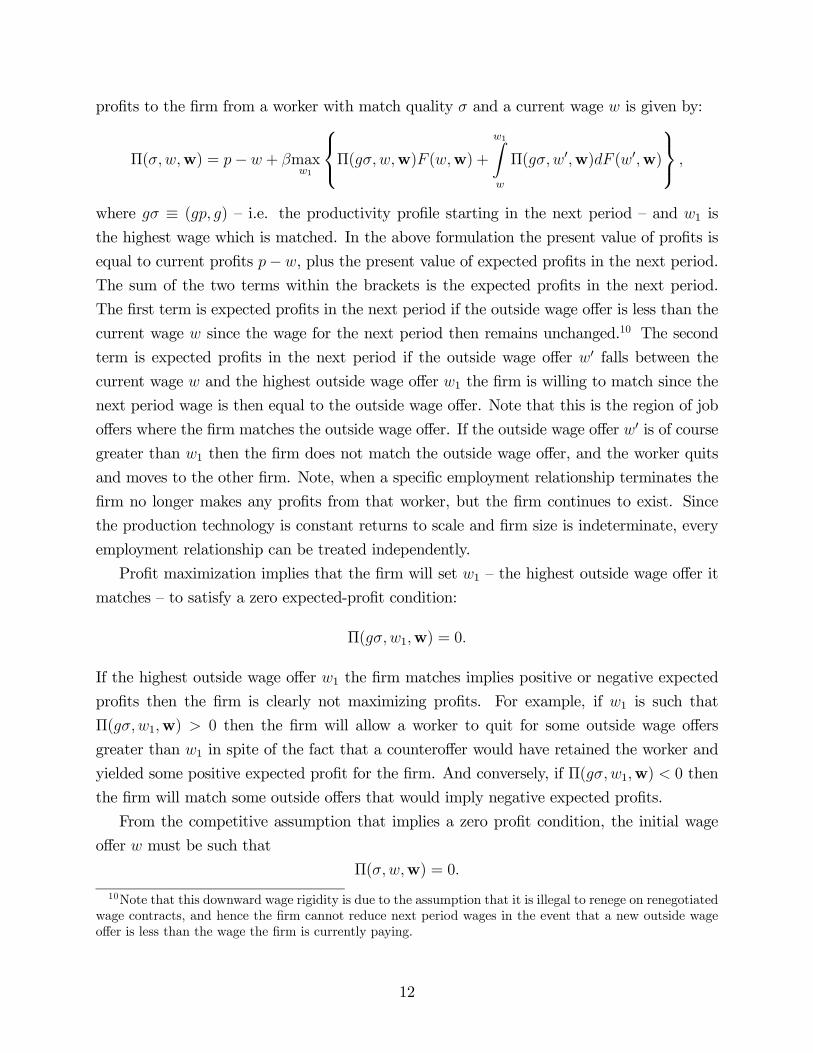
profits to the firm from a worker with match quality σ and a current wage w is given by:

Π(σ,w,w) = p− w + βmaxw1

⎧⎨⎩Π(gσ, w,w)F (w,w) +

w1Zw

Π(gσ,w0,w)dF (w0,w)

⎫⎬⎭ ,

where gσ ≡ (gp, g) — i.e. the productivity profile starting in the next period — and w1 is

the highest wage which is matched. In the above formulation the present value of profits is

equal to current profits p−w, plus the present value of expected profits in the next period.

The sum of the two terms within the brackets is the expected profits in the next period.

The first term is expected profits in the next period if the outside wage offer is less than the

current wage w since the wage for the next period then remains unchanged.10 The second

term is expected profits in the next period if the outside wage offer w0 falls between the

current wage w and the highest outside wage offer w1 the firm is willing to match since the

next period wage is then equal to the outside wage offer. Note that this is the region of job

offers where the firm matches the outside wage offer. If the outside wage offer w0 is of course

greater than w1 then the firm does not match the outside wage offer, and the worker quits

and moves to the other firm. Note, when a specific employment relationship terminates the

firm no longer makes any profits from that worker, but the firm continues to exist. Since

the production technology is constant returns to scale and firm size is indeterminate, every

employment relationship can be treated independently.

Profit maximization implies that the firm will set w1 — the highest outside wage offer it

matches — to satisfy a zero expected-profit condition:

Π(gσ, w1,w) = 0.

If the highest outside wage offer w1 the firm matches implies positive or negative expected

profits then the firm is clearly not maximizing profits. For example, if w1 is such that

Π(gσ,w1,w) > 0 then the firm will allow a worker to quit for some outside wage offers

greater than w1 in spite of the fact that a counteroffer would have retained the worker and

yielded some positive expected profit for the firm. And conversely, if Π(gσ, w1,w) < 0 then

the firm will match some outside offers that would imply negative expected profits.

From the competitive assumption that implies a zero profit condition, the initial wage

offer w must be such that

Π(σ,w,w) = 0.

10Note that this downward wage rigidity is due to the assumption that it is illegal to renege on renegotiatedwage contracts, and hence the firm cannot reduce next period wages in the event that a new outside wageoffer is less than the wage the firm is currently paying.

12

Hence the equilibrium wage function w : Σ −→ R+ must satisfy

Π(σ,w(σ),w) = 0, for all σ.

If w(·) is the equilibrium wage function then the firm’s initial wage offer is w (σ) and the

highest outside wage offer the firm will match at time t is w (gtσ), ∀t > 0, where gtσ ≡(gtp, g). Hence a function w(·) such that Π(σ,w(σ),w) = 0 is the solution to the firm’s

two-fold problem. Note the initial zero-profit equilibrium wage w (σ) is the actual wage paid

to the worker. But the subsequent zero-profit wages over the duration of the employment

relationship — that is, w (gtσ), ∀t > 0 — are simply the highest outside wages the firm wouldbe willing to match and not the wages the firm is forced to pay the worker in every future

period.

The proof of existence of the equilibrium wage function w is by constructing a function

and showing that it satisfies the condition Π(σ,w(σ),w) = 0, for all σ. In order to construct

a candidate wage function, first denote W (σ) as “match value,” and define it as the highest

present value of expected lifetime productivity of a worker with match quality σ:

W (σ) = p+ βEmax {W (gσ),W (eσ)}= p+ β

½W (gσ)φ(eσ|W (eσ) ≤W (gσ)) +

Z{σ|W (σ)>W (gσ)}

W (eσ)dφ(eσ)¾The first result is given in the lemma below.

LEMMA 1. W (σ) exists and it is increasing in p and g.

PROOF. See Appendix.

Match value is the present value of lifetime productivity under a policy of optimal

turnover, and it is clearly an increasing function of the productivity level p and growth

rate g, and hence match value increases as the employment relationship ages. Match value

represents the solution to the social planner’s problem with search frictions and where each

worker-firm match is characterized by an idiosyncratic productivity profile.

The next proposition claims that the zero-profit equilibrium wage function can be explic-

itly defined in terms of current productivity and the difference in future and current match

values.

13

PROPOSITION 1. Given Assumptions 1 to 3, for every σ ∈ Σ and a given φ,

w(σ) = p+ β

((W (gσ)−W (σ))φ(eσ|W (eσ) ≤W (σ))

+R{σ|W (σ)<W (σ)≤W (gσ)}(W (gσ)−W (eσ))dφ(eσ)

)

is the zero-profit equilibrium wage function.

The proof is based on several lemmas. The first lemma states that the candidate equi-

librium wage function given above is a monotone transformation of match value.

LEMMA 2. w(σ) is a monotone transformation of W (σ).

PROOF. See Appendix.

Lemma 2 says that if any two jobs have the same match value then the equilibrium wage

offer will be the same for both jobs, and that if one job has a higher match value than another

job then the equilibrium wage offer will be higher for the first job than for the second job.

In order to prove that this candidate function is in fact the fixed point solution — i.e.

the equilibrium wage function — to the firm’s problem given by Π(σ,w(σ),w) = 0, we need

to characterize the present value of wage payments to a worker under a policy of wage

renegotiation where outside wage offers are determined by the candidate equilibrium wage

function. Denote V (w,w) as “job value,” and define it as the present value of expected

lifetime wage payments to a worker when the firm pays a wage w and the worker receives a

single outside wage offer w(eσ) in every period. Recall, for a given w the CDF of wage offersis given by F (w,w) = φ(eσ|w(eσ) ≤ w). Hence, given a current wage w and equilibrium wage

function w, job value can be expressed as follows:

V (w,w) = w + βEmax {V (w,w), V (w(eσ),w)}= w + β

½V (w,w)φ(eσ|w(eσ) ≤ w) +

Z{σ|w(σ)≥w}

V (w(eσ),w)dφ(eσ)¾The only source of wage increase for the worker is the receipt of a better outside wage

offer. Job value, unlike match value, is independent of the turnover rule since the worker is

indifferent whether a wage increase occurs because the incumbent firm matches an outside

offer or because the worker moves to another firm. Hence job value is only a function of the

current wage w and the distribution of wage offers given by w. Clearly V is a monotonically

increasing function of w.

14

Given the definitions of match value and job value, the following lemma states that the

candidate equilibrium wage function w(σ) is constructed by setting the difference between

match value and job value equal to zero.

LEMMA 3. The function w is such that W (σ)− V (w(σ),w) = 0.

PROOF. Since w(σ) is a monotone transformation of W (σ) (from Lemma 2) we

can write the difference between match value and job value as follows:

W (σ)−V (w(σ),w) = p−w(σ)+β

⎧⎪⎪⎨⎪⎪⎩(W (gσ)− V (w(σ),w))φ(eσ|W (eσ) ≤W (σ))

+R{σ|W (σ)<W (σ)≤W (gσ)}(W (gσ)− V (w(eσ),w)dφ(eσ)

+R{σ|W (σ)>W (gσ)}(W (eσ)− V (w(eσ),w)dφ(eσ)

⎫⎪⎪⎬⎪⎪⎭ .

If W (σ) = V (w(σ),w) for all σ, then by substitution we get:

0 = p−w(σ) + β

⎧⎪⎪⎨⎪⎪⎩(W (gσ)−W (σ))φ(eσ|W (eσ) ≤W (σ))

+R{σ|W (σ)<W (σ)≤W (gσ)}(W (gσ)−W (eσ)dφ(eσ)

+R{σ|W (σ)>W (gσ)}(W (eσ)−W (eσ)dφ(eσ)

⎫⎪⎪⎬⎪⎪⎭ .

Since the last term within the brackets drops out, w(σ) can be expressed as

follows:

w(σ) = p+ β

((W (gσ)−W (σ))φ(eσ|W (eσ) ≤W (σ))

+R{σ|W (σ)<W (σ)≤W (gσ)}(W (gσ)−W (eσ)dφ(eσ)

).

The above function is precisely the same as the candidate equilibrium wage func-

tion considered above.¥

The final step of the proof of Proposition 1 is to show that a firm’s profits are indeed

equal to the difference between match value and job value.

LEMMA 4. A firm’s present value of expected profits from a worker with match

quality σ and current wage w is equal to the difference between match value and

job value: Π(σ,w,w) =W (σ)− V (w,w).

PROOF. Note that W (σ) is the present value of expected lifetime productivity

of a worker given current match quality σ, and V (w,w) is the present value

of expected lifetime wage payments under a policy of wage renegotiation given

15

a current wage w and outside wage offer function w. Hence W (σ) − V (w,w)

is the present value of expected lifetime profits. These aggregate profits are of

course distributed across the current and all the other firms that the worker

could move to in the future. If, however, a worker ever moves to another firm

say with match quality σ0 then the equilibrium wage offer w(σ0) is such that

W (σ0) − V (w(σ0),w) = 0 (from Lemma 3), which implies that the aggregate

expected profit at the time a worker starts working at any new firm is equal to

zero. Hence the present value of expected lifetime profits due to job changes in the

future are clearly equal to zero. Since W (σ)− V (w,w) is simply the discounted

sum of expected profits in the current firm and in all future firms that the worker

could move to, and because the latter is equal to zero, the expected profits of the

firm Π(σ,w,w) =W (σ)− V (w,w).

Moreover, since W (σ) − V (w(σ),w) = 0 (from Lemma 3), w(·) is the solutionto the fixed point problem: Π(σ,w(σ),w) = 0, for all σ, which then completes

the proof of Proposition 1.¥

Hence the candidate function w(σ) defined above in terms of initial productivity and the

difference in future and current match values is the equilibrium wage function that solves the

two-fold problem of the firm. Namely, for a given σ, a firm will make a wage offer w(σ) and

will match any outside wage offer no larger than w(gtσ) in every time period t. Since every

firm uses this same wage function to make their outside wage offers, w(σ) is the zero-profit

equilibrium wage function.

3.3 Properties of the Equilibrium Wage Function

This section analyses some of the properties of the equilibrium wage function. Since every

outside wage offer w(σ) is such thatW (σ) = V (w(σ)) for all σ, and F (w) = φ(eσ|w(eσ) ≤ w),

the equilibrium wage function can be re-written as:11

w(σ) = p+ β

((W (gσ)− V (w(σ)))F (w(σ)) +

Z w(gσ)

w(σ)

(W (gσ)− V (w(eσ)))dF (w(eσ))) .

Under this formulation, the interpretation of the wage premium — given by the discounted

sum of the terms within the bracket — is straightforward. First note that next period profits

are given by W (gσ)− V (w0) if the wage in the next period is w0. The first term within the

bracket is the expected profits in the next period if the outside wage offer is less than the

11For notational brevity, from now on the second argument w in the definitions of V and F are dropped.

16

current equilibrium wage w(σ) — i.e. if the outside wage offer falls in the region where the

wage remains unchanged. The second term is the expected profits in the next period if the

outside wage offer falls between w(σ) and the highest outside wage offer the firm is willing to

match w(gσ) — i.e. if the outside wage offer falls in the wage renegotiation region where the

firm matches the outside wage offer. Hence the sum of these two terms is the expected profits

the firm extracts in the next period because it does not increase wages unless the worker

receives a better outside wage offer. Since the equilibrium wage w(σ) is a zero-profit wage,

these expected future profits that the worker cannot collect in the future must be collected

by the worker as an up-front payment. Put differently, because firms are unable to commit

to future wage increases they must include this compensating up-front wage premium in

their zero-profit equilibrium wage offers.

This equilibrium wage function also generates optimal turnover since the worker will only

move to another firm if the outside job offer has a higher match value than the match value

in the incumbent firm. The result is stated below.

COROLLARY 1. w(·) generates optimal turnover.

PROOF. Profit maximization implies that a firm will allow a worker to quit a

job in the next period if and only if w(gσ) < w(eσ). Since w(·) is a monotonetransformation of W (·) (from Lemma 2) it follows that the worker will quit a

job if and only if W (gσ) < W (eσ) — that is, if the match value of the outside joboffer is greater than the match value in the incumbent firm. Since turnover is

optimal in the definition of match value, the equilibrium wage function w(·) alsogenerates optimal turnover.¥

This result shows that the wage renegotiation policy generates optimal turnover and

thus mimics the social planner’s solution to the allocation of workers among jobs given

search frictions. The efficiency of the market mechanism is due not only to the assumption

that equilibrium wage offers are zero-profit competitive wages, but also because search effort

is exogenous.12

Since match value is increasing in p and g, and job value is increasing in wages, the

equilibrium wage function w(·) is clearly increasing in p and g. Moreover, the wage premiumw(σ)−p is a function of g and match valueW (σ). A higher growth rate implies a higher wagepremium because future productivity is higher and not all of it can be captured by the worker

12If search effort is endogenously determined then this efficiency result no longer holds even though theturnover rule remains optimal. See Section 3.4.3 for a more detailed discussion of this issue.

17

in the future. For instance, in the absence of productivity growth there is no wage premium

since W (gσ) = W (σ) and hence w(σ) = p. Also note that the match value is correlated

with the wage premium. For example, consider a job σ such that W (eσ) ≤ W (σ), ∀eσ — i.e.the job with the highest match value. Then the wage premium is given by: w(σ)− p(σ) =

β[W (gσ) − V (w(σ),w)]. This difference is larger since the renegotiation term drops out.

The intuition for this larger wage premium is that there are no better outside wage offers

the worker can use as leverage to capture future increases in match value. As a consequence,

the entire increase in future rents are collected up-front, which implies a relatively higher

wage premium. Conversely, if σ is the job with the lowest possible match value then the

wage premium is given by:

w(σ)− p(σ) = β

Z{σ|W (σ)<W (σ)≤W (gσ)}

(W (gσ)− V (w(eσ),w))dφ(eσ).Note that every job offer in the next period allows the worker to capture some (if W (gσ) >

W (eσ)) or all (ifW (gσ) ≤W (eσ)) of the increase in future match value. As a consequence, thewage premium given above is relatively small. The point is that the wage premium increases

with match value because it gets harder for the worker to extract rents in the future as match

value increases since the likelihood of better wage offers decreases.

Although outside wage offers must satisfy a zero-profit condition, for an identical σ

the w(σ) could be very different depending on the distribution φ(σ). For instance, if the

distribution of productivity profiles changes so that the likelihood of a better offer for a

given σ increases then the wage premium will be lower. The intuition for this result is that

because it is more likely that the worker will receive a better wage offer, the worker is able

to extract more future rents, and hence the wage premium can be correspondingly smaller.

Clearly, this equilibrium wage depends on both the productivity profile σ and the probability

distribution φ over Σ.13

The explicit formulation of the equilibrium wage function also makes it transparent why

the model here is both an external and internal labor market theory of wages. The equilib-

rium wage is clearly a function of both outside wage offers and productivity increases on the

job. Put differently, the source of within-job wage increases and turnover is the interplay

between “external” wage offers and “internal” productivity growth on the job.

A final comment relates to the endogeneity of the wage offer distribution. The exogenous

feature of the model is a non-degenerate distribution of productivity profiles across all worker-

firm pairs. The model, however, generates an equilibrium wage function that gives rise to13In Gerratana and Munasinghe (2005), we study the properties of this match value function in greater

detail. For example, we look at the effects of changes in φ on the marginal rate of transformation betweenp and g — i.e., the tradeoff between p and g, holding match value constant.

18

the outside wage offer distribution. That is, for every exogenously given σ and distribution

φ there exists an endogenously determined equilibrium wage given by w(σ). Hence although

φ is exogenous the corresponding equilibrium wage offer distribution is endogenous.

Before proceeding to the model implications, Section 3 concludes with a discussion of the

modeling assumptions. The objective here is to try and identify, justify (where possible),

and critically assess the key assumptions of the model.

3.4 Assumptions and Robustness of the Model

3.4.1 Heterogeneity of Firm-Specific Productivity Profiles

The basic presumption of the model is the existence of a non-degenerate distribution of

firm-specific productivity profiles across all worker-firm pairs. This particular rendition of

job matching as a “firm” specific phenomenon is essential to generate model implications

consistent with the employment dimension of the empirical findings — i.e. within-firm wage

dynamics and inter-firm labor mobility — mentioned in Section 2. However, the critical

assumption is not whether the firm is the appropriate demarcation of skill specificity per

se because the applicability of this theoretical framework depends only on whether there

are any employment dimensions — from industry classifications to specialized tasks — along

which skill acquisition may be specific in the sense elaborated here. Some evidence suggests

that skill acquisition on the job may be more industry specific than firm specific (Neal 1995).

Other theoretical work (Gibbons and Waldman 2003) swings the pendulum in the opposite

direction and introduces “task-specific” human capital to explain some features of internal

labor markets. In principle the model here could be adapted to address industry or task

specific skill acquisition and generate implications related industry or internal labor market

compensation and mobility dynamics.

The second, and perhaps novel, aspect of a worker-firm match is that different work

environments offer different opportunities for skill accumulation or on-the-job productivity

growth. Empirical evidence of differences in productivity growth on the job is of course

scarce, even though there is overwhelming evidence of differences in the provision of formal

and informal training.14 However, the idea that different jobs or work activities or occu-

pations offer different learning and growth opportunities (e.g. Rosen 1972; Weiss 1971) are

certainly not new in the labor literature. Also, heterogeneity of skill accumulation is the cor-

14Such provision of training of course should be seen as part of the contractual relationship between theworker and the firm, as is the wage. But that would imply particular correlation patterns between initialwages and productivity growth rates like in Jovanovic (1979b). Hence to impose constraints on the correlationbetween p and g also constraints the array of possible covariance patterns of successive wage increases. Thisissue is discussed further in Section 4.6.

19

nerstone of human capital theory as an explanation of personal income distribution (Mincer

1993). Although the model here generates a variety of basic results on wage and turnover

dynamics holding productivity growth constant, heterogeneity of growth rates is an essential

assumption for deriving some of the more substantive model implications related to wage

growth and turnover, and serial correlation of wage increases.

3.4.2 Competitive Wage Offers

The assumption that outside firms offer a zero-profit competitive wage simplifies the deriva-

tion of the equilibrium wage function and allows an explicit characterization of this wage

function. However, this assumption that firms offer a competitive wage is strong. So the

question is whether there are other reasonable assumptions about the determination of ini-

tial wage offers and whether the modeling results of the paper are robust to alternative

specifications.

The model implicitly assumes that firms have all the bargaining power to set wages once

an employment relationship commences. In the current version of the model, this simplifying

assumption about the division of bargaining power is counter balanced by the assumption

that outside firms offer a take-it or leave-it but, zero-profit competitive wage. The latter

assumption of course removes all monopsony power and shifts lifetime rents to the worker.

So the wage setting mechanism here displays extreme elements of both competition for

prospective workers and firm bargaining power. If the model dispenses with the competitive

assumption without limiting the bargaining power of the firm then firms have both the

bargaining power to set wages and monopsony power to determine initial wages, like, for

example, in Postel-Vinay and Robin (2002). One alternative that avoids both these sets

of extreme assumptions is to relax the competitive assumption and to also give the firm

less bargaining power. A specific proposal is to assume that outside firms have incomplete

information about the productivity profile and current compensation of the worker in the

incumbent firm. Then allowing the firm to have monopsony power in making a wage offer

would be counterbalanced by the fact that the outside firm is disadvantaged because of

this information asymmetry. A wage offer under such a setup would clearly imply positive

profits and is likely to generate implications similar to the model implications of this paper.

The derivation of an equilibrium wage function under these assumptions and analysis of the

welfare properties of this wage function are currently under investigation (Gerratana and

Munasinghe 2005).

In addition to these non-cooperative solutions, there is of course an extensive history

of cooperative solution concepts in the literature on rent sharing. The important point is

that irrespective of the solution we adopt for how initial wage offers are determined, the

20

salient feature of the model that generates wage and turnover dynamics is the assumed

bidding competition between the incumbent firm and outside firm. Hence, as long as within-

job wage dynamics are determined by a policy of wage renegotiation the key qualitative

implications related to within-job wage and turnover dynamics are likely to be robust to

alternative solutions to the problem of initial wage offers.

Different solution concepts for the initial wages however will clearly affect the size of the

up-front wage premium, and clearly the extent of this premium will be a measure of compet-

itiveness for prospective workers in the labor market. If firms offer non-competitive initial

wages that imply positive profits clearly the wage premium will decline and hence initial

wage growth on the job could be correspondingly larger. Note however if wage renegotiation

at any point during an employment relationship leads to a wage close to the highest outside

wage offer the firm is willing to match (i.e. the zero-profit wage) then the expected wage

growth from that point on will again be attenuated for the reasons expounded in the paper.

The more relevant question is whether more detailed empirical studies of wage dynamics in

the early and later periods of an employment relationship can reveal the extent of market

competition for workers.

3.4.3 Exogenous Search

The formal incorporation of search effort into the current framework adds considerable com-

plexity to the modeling details, and hence this important extension is left to a future research

project. However, it is important to highlight some likely ramifications of endogenous search

even though these results are not formally derived here.

Since the model assumes a constant arrival rate of outside job offers, search effort is

not endogenously determined in the model. But of course workers are likely to influence

the arrival rate of outside job offers by searching more or less intensely, and their optimal

effort level will be determined by a benefit-cost analysis of search effort. Under standard

assumptions — an increasing marginal cost function — search effort will be a function of the

wage level since the current wage is a sufficient statistic for job value. Since lower wages

imply higher marginal gains to search, optimal search effort will be a negative function of

current wages. If search effort is a direct function of wages then endogeneity of search will

not alter the qualitative results of the paper because the wage level still remains a sufficient

statistic for job value. As a consequence, the model implications that hold current wages

constant remain robust with endogenously determined search effort.

Although endogenous search effort is unlikely to change the qualitative results of the

paper, it will affect some of the welfare properties of the wage renegotiation policy. In

particular, as Mortensen (1978) observed, a wage policy of matching outside offers will lead

21

to inefficiently high levels of search intensity even though the turnover rule remains optimal.

Since intensity of a worker’s search effort is a function only of the wage the worker receives,

optimal search effort is inefficiently high because the worker does not take into consideration

the capital loss incurred by the firm. In addition, if the offer arrival rate is a function of

the wage level, then wages (turnover) would increase (decrease) more rapidly at lower wage

levels and less rapidly at high wage levels than would be predicted by a constant offer arrival

rate.

A final observation is that with endogenous search effort if workers sample multiple

firms at a time then dispensing with the competitive assumption will still not lead to full

monopsony power. Competition among these multiple firms will lead the firm with the best

match to offer a wage that is zero profits to the second best firm.

4 Model Implications

This section derives various model implications that are consistent with the empirical findings

discussed in Section 2. The first set of implications derived in Section 4.1 relates to the

evolution of wages and worker-firm separation rates over the duration of an employment

relationship. Section 4.2 explicitly incorporates heterogeneity of productivity growth rates

and derives the key intermediate result that the highest outside wage offer a firm matches is

higher in high growth jobs than in low growth jobs, holding match value constant. Section

4.3 compares the implications of wage growth and turnover rates across high and low growth

jobs. Section 4.4 shows that the covariance of successive wage increases is negative for a

given productivity profile, whereas the unconditional covariance is indeterminate. Section

4.5 briefly lists some other noteworthy modeling results, and Section 4.6 concludes with a

discussion of some shortcomings of the paper.

4.1 Wage and Turnover Dynamics

Two immediate implications of the model are: mean wages increase and turnover rates

decrease with job tenure. These results follow directly from the fact that the highest outside

wage offer a firm is willing to match is increasing in p and g. These results are formally

stated in Proposition 1. Denote bwt as the highest outside wage offer the firm would match

at time t where bwt ≡ w(gtσ), and wt as the mean or expected wage at time t.

PROPOSITION 2. (1) Mean wages increase with job tenure: wt+1 > wt,∀t > 0.(2) Turnover rates decrease with job tenure: 1− F (bwt+1) < 1− F (bwt),∀t ≥ 0.

22

PROOF. See Appendix.

Recall that the zero-profit equilibrium wage function w(·) — i.e. the wage function thatdetermines the initial wage and the highest outside wage offers the firm is willing to match

in subsequent time periods — is increasing in p for any given g. Hence this highest outside

wage offer the firm is willing to match increases with tenure because productivity increases

on the job. As a consequence the mean wage increases with tenure turnover decreases with

tenure. These results are graphically illustrated in Figure 1. Note however that the mean

wage increase is smaller than the corresponding increase in the highest outside wage offer

the firm is willing to match since the latter is only the upper bound for a renegotiated wage

contract. But the decrease in the turnover rate corresponds directly to the corresponding

increase in the highest outside wage offer the firm is willing to match. The model therefore

implies the standard dual tenure effects, but the positive tenure effect on wages, unlike

the negative tenure effect on turnover, is attenuated due to the wage renegotiation policy.

These asymmetric tenure effects are consistent with the findings of quantitatively small (and

not always significant) tenure effects on wages and large (and always significant) negative

tenure effects on turnover. Hence a small estimated wage return on tenure should not be

interpreted as necessarily implying a diminished role for specific skill accumulation on the

job. The negative tenure effect on turnover is in fact the more appropriate gauge of specific

skill accumulation.

The model also implies that tenure will be negatively correlated with turnover even if

the current wage is held constant. Recall, turnover is determined by the highest outside

wage offer the firm is willing to match but the current wage always lies somewhere between

this “highest” wage and the initial zero-profit equilibrium wage. As a consequence, consider

the turnover rate one period later if wages remain unchanged due to a low outside wage

offer. Clearly the turnover rate falls because a period later the highest outside wage offer

the firm is willing to match is higher. Hence turnover will decrease with tenure even if

wages are held constant. This result is clearly consistent with the empirical observation that

turnover decreases with tenure despite holding the wage constant (Topel and Ward 1992).

As mentioned in Section 2, matching models are unable to reconcile this fact because they

predict turnover will increase with tenure if wages are held constant.

4.2 High and Low Growth Jobs

This section introduces high and low productivity growth jobs and derives a key intermediate

result that underpins various modeling results related to wage growth, turnover, and serial

23

correlation of wage increases. First, denote a high growth job as σH0 ≡ (pH , gH), and a lowgrowth job as σL0 ≡ (pL, gL), where gH > gL. Assume that both jobs have the same match

value at the time of job start, i.e. W (σH0 ) = W (σL0 ). Hence both jobs have the same initial

zero-profit equilibrium wages. Since W (σH0 ) = V (w(σH0 )) and V (w(σL0 )) = W (σL0 ), and V

is a monotonically increasing function of wages, w(σH0 ) = w(σL0 ). This implies (the result

is formally stated below) that the highest outside wage offer a firm is willing to match is

higher in the high growth job than in the low growth job in all subsequent time periods. Let

σJt ≡ ((gJ)tpJ , gJ) for J = H and L, and for notational simplicity denote bwH0 (≡ w(σH0 )) andbwL

0 (≡ w(σL0 )) as the initial equilibrium wages, and bwHt (≡ w(σHt )) and bwL

t (≡ w(σLt )) as thehighest outside wage offers a firm would match at time t, in the high and low growth jobs,

respectively.

LEMMA 5. If bwH0 = bwL

0 then bwHt > bwL

t , ∀t > 0.

PROOF. Since match value is a function of the growth rate it follows that:

If W (σH0 ) =W (σL0 ) then W (σHt ) > W (σLt ), ∀t > 0,

since gH > gL. The match value of the high growth job increases faster than

the match value of the low growth job. Note bwHt and bwL

t must satisfy W (σHt ) =

V (bwHt ) and W (σLt ) = V (bwL

t ), respectively. Since W (σHt ) > W (σLt ) and V is

monotonically increasing in wages, bwHt > bwL

t , ∀t > 0. ¥

This result underpins the various model implications related to wage growth, turnover,

and serial correlation of wage increases derived in the next two subsections.

4.3 Wage Growth and Turnover

The following proposition states that the mean wage is higher and turnover is lower in the

high growth job than in low growth job, holding the initial zero-profit equilibrium wage

constant — i.e. bwH0 = bwL

0 . Denote wHt and wL

t as the mean wages at time t in the high and

low growth job, respectively.

PROPOSITION 3. (1) Mean wage is higher in the high growth job than in the

low growth job: wHt > wL

t ,∀t > 0. (2) Turnover rate is lower in the high growthjob than in the low growth job: 1− F ( bwH

t ) < 1− F ( bwLt ), ∀t > 0.

PROOF. See Appendix.

24

Both items in Proposition 3 follow from Lemma 5. The turnover result needs the addi-

tional assumption that workers in both jobs sample outside wage offers from same distrib-

ution in every period. These results are graphically illustrated in Figure 2. Note, although

both jobs have the same match value (and hence the same initial zero-profit, equilibrium

wages at the time of job start), it does not imply that the expected sum of productivities in

the two jobs are the same. Recall, match value refers to the present value of lifetime produc-

tivity that includes not only expected productivity in the incumbent job but also expected

productivity in outside firms (due to future mobility). In the high growth job expected pro-

ductivity in the current firm is larger than it is in the low growth job, holding match value

constant.

The important empirical corollary of Proposition 3 is that past wage growth on a job is

negatively correlated with quit rates since average wage growth is higher in high growth jobs

than it is in low growth jobs. This implication addresses a key finding in the literature that

jobs offering higher wage growth are significantly less likely to end in worker-firm separations

than jobs offering lower wage growth, holding the current wage constant (Topel and Ward,

1992). The precise finding is that in a turnover regression both the initial wage and current

wage have significant positive and negative coefficient estimates, respectively. Note that on

the basis of the model, the wage at time t is not a precise proxy for match value at time

t, but holding the initial equilibrium wage constant, the current wage is a proxy for wage

growth, and hence the current wage is positively related to match value. Similarly, holding

the current wage constant, the initial wage is also a proxy, albeit negatively, for wage growth,

and thus the initial wage is negatively related to match value. Hence the model is consistent

with the observed findings of a negative effect of initial wages and a positive effect of current

wages on turnover.

4.4 Serial Correlation of Wage Increases

Although productivity increases on the job are deterministic, within-job wage increases fol-

low a stochastic process because firms increase wages if and only if the worker receives a

better outside wage offer. As a consequence, the model implications for serial correlation

of wage increases are more complex despite productivity increases that are positively cor-

related by assumption. More specifically, for a given productivity profile the covariance of

successive wage increases is negative, whereas the same covariance without the conditioning

is indeterminate. The latter result resolves the paradox on wage growth heterogeneity.

For expositional convenience, consider the wage renegotiation policy in two consecutive

time periods. Let bw1 be a random variable and define a second random variable as bw2 =25

(1 + α)bw1, where α > 0. Interpret bw1 and bw2 as the highest outside wage offers thata firm matches in the two periods immediately following employment. Denote bw0 as theinitial equilibrium wage, and note bw0 < bw1. If bw0 is a constant then sequences given by{bw0, bw1, bw2} mimics various productivity profiles of equivalent match value. A higher drawfrom bw1 simply refers to a steeper productivity profile — i.e., to a higher g. The covarianceof successive increases in the highest outside wage offers a firm is willing to match is positive

by construction:

Cov( bw1 − bw0, bw2 − bw1) = αV ar(bw1) > 0.Note the reason for this positive covariance is the assumption of a positive covariance of

successive increases in the underlying productivity.

Next, denote X1 and X2 as the wage offers in periods 1 and 2, respectively, from a

stationary distribution. Let w1 and w2 be the observed wages in periods 1 and 2 due to the

wage renegotiation process. In the first period, ifX1 ≤ bw0 then w1 = bw0 and if bw0 < X1 ≤ bw1then w1 = X1; in the second period, if X2 ≤ w1 then w2 = w1 and if w1 < X2 ≤ (1 + α)bw1then w2 = X2. If either X1 > bw1 or X2 > bw2 then such observations will not be sampledbecause the worker would have quit and gone to a new firm. The following proposition states

the main result.

PROPOSITION 4. (1) For a given productivity profile the covariance of suc-

cessive wage increases is negative: Cov(w1 − bw0, w2 − w1) < 0, for a given

{bw0, bw1, bw2}. (2) The unconditional covariance however is indeterminate: Cov(w1−bw0, w2 − w1) T 0.

PROOF. See Appendix.

The intuition behind the first item of this proposition is that the first period wage is the

lower bound for the second period wage. So if the wage increase is small in the first period

then the scope for wage increase in the second period is relatively high, and vice versa. As

a consequence the expected wage increase in the second period is negatively related to the

first period wage increase, implying that within-job wage increases are negatively correlated

for any given productivity profile. This intuition is illustrated in Figure 3.

The second item of Proposition 4 may appear counter intuitive since for any given produc-

tivity profile the covariance is negative. However, if observations from high and low growth

jobs are combined the covariance between first period wage increases and second period

wage increases becomes indeterminate for a purely statistical reason. Note, the covariance

26

measures the linear association between the deviations of two random variables from their

respective means. Since the means for first period and second period wage increases change

when populations with different growth rates are combined, the covariance of successive wage

increases becomes indeterminate. Figure 4 attempts to illustrate.

The exact sign of this unconditional covariance for a given φ will depend on which of the

following two countervailing forces dominate. The first is of course the negative correlation

of successive wage increases for a given productivity profile — i.e. item (1) of Proposition

4. A lower growth rate is likely to result in a smaller negative correlation because it makes

zero wage increases in successive periods more likely. Also a higher match value will tend

to reduce this negative correlation because a high match value implies a lower probability of

receiving a higher outside wage offer. These factors that make small or zero wage increases

in successive periods more likely will tend to attenuate this negative correlation. Put simply,

a productivity profile with a high growth rate or low match value will imply a stronger

negative correlation of successive wage increases.

The second positive effect is due to the extent of heterogeneity of productivity growth

rates holding match value constant. Clearly the means of wage increases in successive periods

will be positively correlated given heterogeneity of productivity growth rates. In terms of

the basic elements of the model, if p and g are positively correlated then holding match value

constant would imply little variation in observed growth rates, which in turn would attenuate

this positive effect on the covariance of successive wage increases.15 However, if p and g are

negatively correlated then holding match value constant would nevertheless generate a large

variation in g, and thus a large positive effect on the unconditional covariance term. Hence

the distribution of p and g will critically determine the size of this positive effect on the

unconditional covariance. In conclusion, the exact sign of covariance of wage increases in

successive periods without conditioning on the growth rate, will of course depend on which

of these two countervailing forces dominate.

To address the empirical results on serial correlation of wage increases, note one impli-

15The correlation between p and g, or its equivalent counterparts, has been investigated both theoreticallyand empirically. As mentioned earlier, if g was endogenously determined by p like in Jovanovic (1979b) thenholding match value constant would imply no variation in g at all. On the other hand, different on-the-joblearning opportunities combined with equilibrium considerations could imply a negative correlation betweenbetween p and g. For example, Becker (1975) and Mincer (1993) have argued that labor mobility will leadto equalization of present values among jobs with different learning opportunities, and Hause (1980), usingSwedish data, estimated a wage model that implied a negative correlation between the individual constantterm and slope. These latter studies suggest a negative correlation between p and g.A similar idea can also be found in the literature on the adoption of new technologies. As Parente

(1993) writes, “The firm faces a tradeoff in its choice of technologies to adopt. The more advanced the newtachnology is, the greater its productive potential, but smaller the firm’s starting level of expertise in thattechnology.” The comparative static exercise in this paper also implies a similar tradeoff between currentproductivity and growth rate of productivity.

27

cation of item (1) in Proposition 4 is that if heterogeneity of permanent wage growth rates

among jobs is unimportant, as Topel and Ward (1992) claim, then the model predicts a neg-

ative covariance of successive wage increases, which they do not find in their data. The key

theoretical point, however, is the indeterminacy of serial correlation of wage increases despite

the fact that productivity increases are serially correlated by construction, which implies that

serial correlation of wage increases is an inconclusive test of differences in permanent rates

of wage growth among jobs. Hence studies that fail to find positive serial correlation of

wage increases such as Topel (1991) and Topel and Ward (1992) do not necessarily present

evidence against the hypothesis of heterogeneity of permanent differences in wage growth

rates among jobs. More important, Propositions 3 and 4 jointly solve one of the empirical

riddles that motivated the paper: past wage growth reduces turnover and yet the same data

fail to show any evidence of serial correlation of wage increases. The model explains why

positive serial correlation of wage increases is not a necessary implication of heterogeneity

of permanent wage growth rates among jobs.

4.5 Other Implications

The search-and-matching and wage renegotiation features of the model directly imply some

other well-known results related to wages and labor mobility. For example, wage increases

and turnover decreases over the individual life cycle are direct implications of models with

search frictions. The model presented here implies that wages increase and turnover rates

decrease with labor market experience. Workers who have been in the labor market for a long

time are more likely to have found better jobs with higher wages and as a consequence are

less likely to turnover in the future. These patterns are widely documented in the empirical

literature.

On a related note, the model also predicts positive wage gains when workers change

employers. Note, firms offer zero-profit equilibrium wages and workers only quit when they

receive a wage offer that is higher than the maximum wage the incumbent firm is willing to

match. As a result, mobility wage gains conditional on a quit — the difference in first period

wages in a new firm and last period wages in the old firm — are always positive. Evidence

shows that wage gains of movers are positive especially among those who “quit” their jobs

(Mincer 1986).

Job matching models generate equilibrium wage dispersion. Since matching with het-

erogeneous growth rates and wage renegotiation create more complex wage outcomes, the

model here generates wage dispersion even if observed and unobserved worker and job char-

acteristics such as tenure, experience, and match quality are held constant. The reason is

28

that wage renegotiation creates an essential indeterminacy of current wages that must lie

between the equilibrium wage and the highest outside wage offers the firm is willing to match

in future time periods. Hence wage dispersion is not simply a consequence of heterogeneous

match quality, but it also driven by firm specific productivity growth and the policy of wage

renegotiation.16

A final noteworthy implication of wage renegotiation is the cluster of observations at zero

nominal within-job wage changes. If an outside wage offer is less than current wages, the next

period wage remains unchanged. As a consequence, the model predicts a cluster of exactly

zero nominal wage changes. McLaughlin (1994) presents evidence, from the Panel Study

of Income Dynamics (1976-1986), of nominal wage changes of those staying with the same

employer, where the striking feature is indeed the large cluster of observations at precisely

the point of zero nominal changes. Baker et al. (1994) also show that among a sample of

managerial employees a significant proportion of them receive precisely zero nominal salary

increases.

4.6 Some Shortcomings

Since one of the main motivations for this study is to replicate properties of individual wage

and turnover data, the absence of a quantitative evaluation of the model is a limitation of the

paper. In particular, the model implications for the quantitative effects of tenure on wages

and turnover, and the sign of the covariance of wage increases in adjacent time periods depend

crucially on the distribution of p and g among jobs As a consequence, a simulation exercise to

determine some the joint distributions of p and g that could generate quantitatively sensible

results is an important extension and validation of the theory elaborated in this paper. In

an on-going companion paper (Gerratana and Munasinghe 2005), one clear focus is to bridge

the gap between this theory and an empirical evaluation of the model.

Clearly the model presented here does not address other well documented facts about

wages and turnover. For example, although the evidence on mobility wage gains conditional

on a quits is largely positive, there is nevertheless a substantial fraction of job-to-job changes

that are associated with a wage cut, which is inconsistent with the model. A model where a

firm pays a worker her marginal product in every period would indeed generate such a result.

16These results are comparable to the results in Burdett and Coles (2003) where there is both initial wagedispersion and wage increases with tenure. They obtain these results within the context of homogeneousfirms and workers, because in part what they want to explain is wage dispersion across worker who areobservationally equivalent. The model presented here of course assumes heterogeneity of match quality acrossworker-firm pairs. But note that under this assuption workers are nonetheless observationally equivalent.For a recent and thorough survey of wage dispersion in search-theoretic models of labor markets see

Rogerson et al. (2004).

29

A worker moving to a high growth job would be willing to take a wage cut in anticipation

of receiving higher wages in the future. Moreover, the assumed downward wage rigidity

of the model is also inconsistent with some evidence that shows within-job wage cuts are

not uncommon (Baker, Gibbs and Holmstrom 1994) and negative wage returns to tenure

(Ransom 1993).

A final set of observations is that since the model does not assume general productivity

growth, it is silent about returns to general skills or general labor market experience. Hence

the vast empirical literature on estimating wage returns to experience and general skills is not

addressed in this paper. Also the theory presented here only models job-to-job transitions

and does not address unemployment, which is one of the central topics addressed in the

search literature.

5 Related Theory

Themodel in this paper is closely related to the theoretical literature on search-and-matching,

specific human capital, and wage renegotiation. Since Becker’s original idea of sharing costs

and returns of firm specific investments as a means of providing mutual insurance to each

party’s investment, the problem of wage determination has been well known (Becker 1962;

Parsons 1972; Hashimoto 1981). Although the inherent inefficiency of Becker-type sharing

rules was recognized from the beginning, Mortensen (1978) is the first to explicitly consider

employment agreements that would induce both workers and employers to pursue efficient or

joint wealth maximizing search strategies. In particular, Mortensen considers two such wage

setting mechanisms: first, matching alternative offers obtained by one’s partner, and second,

ex ante agreement by each party to compensate the other as a precondition for separation.

He shows counteroffer matching implies an efficient turnover rule if on-the-job search is ex-

ogenous. With endogenous search effort, although the turnover rule remains efficient, each

party still has an incentive to search too intensively. The second employment agreement of

contingent compensation leads to both an efficient turnover rule and efficient search effort,

and thus it is joint wealth maximizing.

The wage setting mechanism in this paper is based on Mortensen’s idea of matching

alternative offers.17 In addition, by considering only the case of exogenous worker search,

17Since Mortensen, the idea of wage renegotiation following an outside offer has been widespread. Forexample, the internal wage setting mechanism of Harris and Holmstrom (1982) is based on the idea ofrenegotiation: firms promise to pay a rigid wage until the worker receives a better offer from the marketat which point the old contract is cancelled and a new contract is made which matches the market offer.Also Malcomsom’s (1997) review article on the general issue of contracts and holdup presents various otherapplications of wage renegotiation.

30

the form of the employment agreement adopted here is a simpler version of Mortensen.

As a consequence, the analysis of wage dynamics is more tractable, and the turnover rule

implied by wage renegotiation is efficient for exactly the reasons expounded by Mortensen.

The key difference with Mortensen’s seminal work is the analysis of the equilibrium wage

function. Although in principle Mortensen’s framework might be general enough to allow

match productivity to vary over time, this possibility is not developed into an analysis of

wage determination. In particular, the absence of an equilibrium wage function implies that

Mortensen’s framework cannot generate wage dynamics. In contrast, the model here by

imposing structure on productivity changes on the job and by introducing a competitive

setting is able to explicitly derive an equilibrium wage function. Of course, Mortensen’s

objectives — to analyze efficient employment agreements in the presence of specific rents and

search frictions — are different from the more immediate objectives of this paper — to develop

a theory consistent with a wide range of facts related wage and turnover dynamics.

In a recent work, Postel-Vinay and Robin (2002) also adopt wage renegotiation as their

wage setting mechanism. As a consequence, their model and the one here share some common

features including within-job wage dynamics. The key difference, apart from the fact that

their model addresses unemployment, is the determination of first period equilibrium wages.

In Postel-Vinay and Robin, firms pay unemployed workers only their reservation wage, and

if workers are employed then firms pay only the minimum wage just sufficient to lure workers

away from their incumbent employers. Thus firms collect maximal rents in contrast to the

model here where all expected rents go to the worker. Further, their model allows for wage

cuts when workers voluntarily move to a firm that is likely to be more aggressive in matching

outside offers in the future. However, heterogeneity of firm-specific productivity growth is

not a feature of Postel-Vinay and Robin’s model, and thus it is not explicitly designed to

address implications related to wage growth and turnover, and serial correlation of wage

increases.

The introduction of productivity growth into the Mortensen type wage renegotiation

framework makes this paper similar to Jovanovic (1979b) since it is one of the first the-

oretical articles explicitly to integrate specific human capital theory into a search-and-

matching framework. Put differently, this paper can be viewed as a “Jovanovic (1979b)

meets Mortensen (1978)” type model. In Jovanovic’s model, the level of match quality de-

termines expected job duration which in turn jointly determines optimal search effort and

investment in firm specific human capital. Thus match quality is positively correlated with

productivity growth on the job. Jovanovic’s central result is that turnover declines with

tenure. The key theoretical difference, however, is in the wage setting mechanism. In Jo-

vanovic’s model the employer makes a wage offer to the worker that is equal to marginal

31

product. The justification for such a wage policy is based on reputation repercussions. As Jo-

vanovic says, “employers offering wages below marginal product will acquire bad reputations

and will consequently not be sampled by workers” (p. 1249, Jovanovic 1979b). But firms

unable to commit to future wage increases will have to offer time consistent wage policies.

The policy of wage renegotiation considered here is immune to charges of time inconsistency.

The on-the-job search aspect of the model is based on imperfect information about the

location of the best match as in Burdett (1978). In all adaptations of search-and-matching

models, including Burdett’s, productivity level is a sufficient statistic for job value. In

this paper, however, each worker-firm pair is characterized by an idiosyncratic firm-specific

productivity profile, and the match value of a job increases with time on the job due to

productivity growth. Embedding firm-specific productivity growth within a job matching

framework generates implications for within-job wage and turnover dynamics, unlike Bur-

dett’s model that only generates implications for wage changes due to job switches and

turnover dynamics over the life cycle.

This paper falls within the literature on search-theoretic equilibrium models of labor

markets, and it is closely allied with various recent models of on-the-job search models such

as Burdett and Mortensen (1998), Postel-Vinay and Robin (2002), and Burdett and Coles

(2003), to mention only a few. All these models, like the model in this paper, are based on

non-cooperative solutions to the problem of wage determination when employment relation-

ships generate firm-specific rents. These models also generate wage dispersion even when

workers and firms are homogeneous, and hence they contrast sharply with other standard

models of search that is based on the Nash bargaining solution to the surplus-splitting prob-

lem.18 Note, however, that in a recent paper Shimer (2004) shows that Nash bargaining can

lead to similar wage dispersion results as the wage posting model of Burdett and Mortensen

(1998).

Some of the best known theories of compensation and labor mobility incorporate vari-

ous features of “learning” over the duration of an employment relationship. For example,

Jovanovic’s (1979a) mismatch theory of turnover is based on learning about match quality.

Other seminal contributions to the theory of wage dynamics — e.g. Harris and Holmstrom

(1982), Waldman (1984), Ricart I Costa (1988), and Farber and Gibbons (1996) — are based

on learning about worker ability. The model here does not include any such feature of

learning. However, it is potentially worth considering whether learning about productivity

profiles (i.e. treating a match as an experience good) or learning about unknown worker

ability might lead to other potentially interesting implications.

18See Rogerson et al. (2004) for an excellent survey of this large literature on search-theoretic models ofthe labor market.

32

On a related note, two recent articles by Gibbons and Waldman (1999) and Chiappori et

al. (1999) have proposed models of learning about worker ability to explain a host of findings

on wage and promotion dynamics. The Gibbons-Waldman model is specifically designed to

explain various aspects of internal labor markets documented by Baker et al. (1994). As

mentioned earlier in Section 2, Chiappori et al. derive a late-beginner property of models

characterized by learning and downward wage rigidity, and they confirm various predictions

related to wage and promotion dynamics using personnel data on executives of a French

state-owned firm.19 Unlike the model presented here, neither of these models focus on firm

level turnover. However, an interesting issue is whether promotion dynamics can be derived

in the context of the model presented here by incorporating different job levels. If firm specific

skills are required to move from one job level to the next higher job level, then indeed wage

increases are likely to predict future promotions, an implication explicitly derived in Gibbons

and Waldman. However, if promotions also signal higher general skills, such as managerial

talent to competitor firms, then turnover implications following a promotion are likely to be

amended. More work on the empirical relationships between promotions, wages and turnover

will suggest whether the theory here might be a suitable framework to analyze internal labor

market phenomena.

6 Conclusion

The paper presents a model of within-job wage and turnover dynamics based on firm-specific

productivity increases on the job, search frictions, and wage renegotiation. In summary, wage

increases occur because firms match outside wage offers, and on-the-job search provides the

impetus for within-job wage increases. Average wage increases are higher in high growth

jobs because they generate more firm specific rents. Past wage growth on a job negatively

predicts quits because turnover is lower in high growth jobs than in low growth jobs. A

further implication of the model is that for a given productivity profile the covariance of

successive wage increases is negative, whereas the same covariance without the conditioning

is indeterminate. These results are consistent with a wide range of findings related to wage

and turnover dynamics.

The model in this paper shows that tests of serial correlation of wage increases are

19The model presented in this paper can also generate a result very similar to the late-beginner property:w1 is negatively related to w3 if w2 is held constant. If w1 is lower because of a low match value and w2 isrelatively high because of a high outside wage offer then the predicted wage increase in the following timeperiod is lower because the scope for future wage increase is limited (see item (1) of Proposition 3). This ofcourse implies a lower w3. The only difference between the late-beginner property of LDR models is thatit also holds w0 constant whereas the argument here presumes that w1 is the initial zero-profit equilibriumwage.

33

inconclusive about heterogeneity of permanent rates of wage growth among jobs. The model

also shows that average wage growth is higher in high growth jobs than in low growth jobs.

A joint implication of these two results is that wage increases over a short duration of tenure

are likely to be noisy, and hence less informative about permanent wage growth rates. It

should also be noted that although longer panels provide more accurate information, they

are likely to over sample high growth jobs because they are more likely to survive. Hence,

variance estimates of wage growth measures from longer panels are likely to underestimate

true heterogeneity of growth rates among jobs.

The over sampling of high wage growth jobs also has implications for Topel’s (1991)

two-step procedure for estimating returns to experience and tenure. In the first step Topel

computes the within-job wage growth rate and argues that it is an unbiased estimate of the

joint returns to tenure and experience. However, if high wage growth jobs are more likely

to be over sampled in individual survey data then it would lead to biased estimates. This

selection problem is rarely addressed in the empirical literature. Even when it is recognized

as a potential source of bias, the lack of evidence of serial correlation of wage growth it put

forth as a reason for its empirical irrelevance (e.g., Topel 1991; Altonji and Williams 1997).

What the theory here shows is that serial correlation of wage growth is an inconclusive test of

wage growth heterogeneity. Hence it is doubtful whether Topel’s first step yields an unbiased

estimate of the joint returns to tenure and experience.

This selection bias is further compounded by the fact that the observed wage growth

on the job is an underestimate of firm specific productivity growth. Note that the wage-

tenure profile will be flatter on average with a policy of wage renegotiation compared to

the underlying productivity profile. Thus, estimates of returns to tenure are likely to always

underestimate the true returns to firm specific skills. The point is that the empirical estimates

of wage returns to tenure should not be interpreted as the true returns to the acquisition of

firm specific skills — the initial wage may well represent an up-front payment to the future

acquisition of specific skills.

In the model outside job offers act as means for workers to extract a share of employment

rents. An interesting empirical implication is whether within-job wage growth rates are lower

in less competitive labor markets like in small cities and rural areas. A corollary is that

workers in less competitive labor markets will need to resort to alternative schemes to extract

a share of rents. For example, are unions more likely to be formed in less competitive labor

markets? Is the union wage premium a rent or front-loaded compensation for accumulation

of firm specific skills in the future?

The model here may also be consistent with observed wage adjustments over the business

cycle. For example, Beaudry and DiNardo (1991) find that current wages are negatively

34

correlated with the lowest realized unemployment rate since workers began with their present

employer, whereas the current unemployment rate and the unemployment rate at the time

of job start have a smaller impact. Wage renegotiation implies upward wage revision due

to receipt of better outside wage offers, and clearly a low unemployment rate increases the

likelihood of receiving better outside wage offers. Since employment relationships have rents

over and above the current wage, it is not surprising that the lowest unemployment rate

over the duration of employment has a significantly larger impact on current wages. During

periods of high wage offers wages will renegotiated up and during periods of less labor demand

wages are more likely to be sticky.

7 Appendix

PROOF OF LEMMA 1. Since the proof follows standard dynamic programming techniques

only a sketch of the proof is given. A more detailed version of the proof is available from the

author.

Define the operator ΓW (σ) from the space C (Σ) of continuos functions with domain Σ

as:

ΓW (σ) = p+ β

⎧⎪⎨⎪⎩W (gσ)φ(eσ|W (eσ) ≤W (gσ)) +

Z{σ|W (σ)>W (gσ)}

W (eσ)dφ(eσ)⎫⎪⎬⎪⎭ .

The space of C (Σ) is a Banach space (see for example, Stokey and Lucas, 1989, Chapter

3). Γ : C (Σ) → C (Σ). Moreover, since ΓW (σ) is a contraction, the contraction mapping

theorem implies the existence and uniqueness of W (σ) given by:

W (σ) = p+ β

⎧⎪⎨⎪⎩W (gσ)φ(eσ|W (eσ) ≤W (gσ)) +

Z{σ|W (σ)>W (gσ)}

W (eσ)dφ(eσ)⎫⎪⎬⎪⎭ .

The stationary policy correspondence can be represented as a preference relation over Σ

(i.e. a complete order): σ Â σ0 iff W (σ) > W (σ0). Simple inspection shows that W (σ) is

strictly increasing in p and g.

PROOF OF LEMMA 2. To show that w(σ) is a monotone transformation of W (σ)

consider σ, σ0 ∈ Σ. Then we need to show: (1) If W (σ) = W (σ0) then w(σ) = w(σ0), and

(2) if W (σ) > W (σ0) then w(σ) > w(σ0).

(1) For σ, σ0 ∈ Σ, if W (σ) =W (σ0) then w(σ) = w(σ0).

35

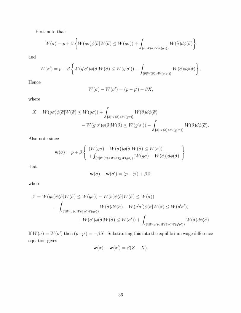
First note that:

W (σ) = p+ β

½W (gσ)φ(eσ|W (eσ) ≤W (gσ)) +

Z{σ|W (σ)>W (gσ)}

W (eσ)dφ(eσ)¾and

W (σ0) = p+ β

½W (g0σ0)φ(eσ|W (eσ) ≤W (g0σ0)) +

Z{σ|W (σ)>W (g0σ0)}

W (eσ)dφ(eσ)¾ .

Hence

W (σ)−W (σ0) = (p− p0) + βX,

where

X =W (gσ)φ(eσ|W (eσ) ≤W (gσ)) +

Z{σ|W (σ)>W (gσ)}

W (eσ)dφ(eσ)−W (g0σ0)φ(eσ|W (eσ) ≤W (g0σ0))−

Z{σ|W (σ)>W (g0σ0)}

W (eσ)dφ(eσ).Also note since

w(σ) = p+ β

((W (gσ)−W (σ))φ(eσ|W (eσ) ≤W (σ))

+R{σ|W (σ)<W (σ)≤W (gσ)}(W (gσ)−W (eσ))dφ(eσ)

)

that

w(σ)−w(σ0) = (p− p0) + βZ,

where

Z =W (gσ)φ(eσ|W (eσ) ≤W (gσ))−W (σ)φ(eσ|W (eσ) ≤W (σ))

−Z{σ|W (σ)<W (σ)≤W (gσ)}

W (eσ)dφ(eσ)−W (g0σ0)φ(eσ|W (eσ) ≤W (g0σ0))

+W (σ0)φ(eσ|W (eσ) ≤W (σ0)) +

Z{σ|W (σ0)<W (σ)≤W (g0σ0)}

W (eσ)dφ(eσ)IfW (σ) =W (σ0) then (p−p0) = −βX. Substituting this into the equilibrium wage differenceequation gives

w(σ)−w(σ0) = β(Z −X).

36

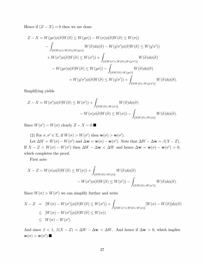
Hence if (Z −X) = 0 then we are done.

Z −X =W (gσ)φ(eσ|W (eσ) ≤W (gσ))−W (σ)φ(eσ|W (eσ) ≤W (σ))

−Z{σ|W (σ)<W (σ)≤W (gσ)}

W (eσ)dφ(eσ)−W (g0σ0)φ(eσ|W (eσ) ≤W (g0σ0))

+W (σ0)φ(eσ|W (eσ) ≤W (σ0)) +

Z{σ|W (σ0)<W (σ)≤W (g0σ0)}

W (eσ)dφ(eσ)−W (gσ)φ(eσ|W (eσ) ≤W (gσ))−

Z{σ|W (σ)>W (gσ)}

W (eσ)dφ(eσ)+W (g0σ0)φ(eσ|W (eσ) ≤W (g0σ0)) +

Z{σ|W (σ)>W (g0σ0)}

W (eσ)dφ(eσ).Simplifying yields

Z −X =W (σ0)φ(eσ|W (eσ) ≤W (σ0)) +

Z{σ|W (σ)>W (σ0)}

W (eσ)dφ(eσ)−W (σ)φ(eσ|W (eσ) ≤W (σ))−

Z{σ|W (σ)>W (σ)}

W (eσ)dφ(eσ).Since W (σ0) =W (σ) clearly Z −X = 0.¥

(2) For σ, σ0 ∈ Σ, if W (σ) > W (σ0) then w(σ) > w(σ0).

Let ∆W =W (σ)−W (σ0) and ∆w = w(σ)−w(σ0). Note that ∆W −∆w = β(X −Z).

If X − Z < W (σ) −W (σ0) then ∆W − ∆w < ∆W and hence ∆w = w(σ) − w(σ0) > 0,

which completes the proof.

First note

X − Z =W (σ)φ(eσ|W (eσ) ≤W (σ)) +

Z{σ|W (σ)>W (σ)}

W (eσ)dφ(eσ)−W (σ0)φ(eσ|W (eσ) ≤W (σ0))−

Z{σ|W (σ)>W (σ0)}

W (eσ)dφ(eσ).Since W (σ) > W (σ0) we can simplify further and write

X − Z = [W (σ)−W (σ0)]φ(eσ|W (eσ) ≤W (σ0)) +

Z{σ|W (σ0)<W (σ)<W (σ)}

[W (σ)−W (eσ)]dφ(eσ)≤ [W (σ)−W (σ0)]φ(eσ|W (eσ) ≤W (σ))

≤ W (σ)−W (σ0).

And since β < 1, β(X − Z) = ∆W − ∆w < ∆W . And hence if ∆w > 0, which implies

w(σ) > w(σ0).¥

37

PROOF OF PROPOSITION 2. To show that average wages increase with tenure, first

define the expected wage at time t+ 1 conditional on wage wt at time t as:

wt+1|wt = αwt + (1− α)

Z wt+1

wt

wdF (w) > wt,

where α = F (wt)/F (bwt+1). Since wt+1|wt is greater for every possible previous period wage

wt, it follows that wt+1 > wt.

The turnover result follows because the highest wage the firm is willing to match increases

with tenure, i.e. bwt+1 > bwt,∀t ≥ 0, and F is a strictly increasing function.

PROOF OF PROPOSITION 3. The first item claims that the expected wage in the high

growth job is higher than the expected wage in the low growth job. Since the start wage is

the same in both jobs, it implies that the expected wage growth is higher in the high growth

job. This proposition is proved by induction. Note that if the distribution of wages in the

high growth job stochastically dominates the wage distribution in the low growth job (for

time periods greater than 0), Proposition 3 follows trivially. First a lemma, to be used in

the induction proof, is established. Second, stochastic dominance of the wage distribution in

the high growth is proved for t = 1. Finally, stochastic dominance is assumed for t = n, and

it is shown that stochastic dominance holds for t = n+ 1, which then concludes the proof.

Define a r.v. X from the distribution as F . Next define two further r.v.s, RL and RH ,

such that:

RL = X if a1 < X ≤ b1

= a1 if X ≤ a1

=∞ if X > b1, a1 < b1

and similarly for RH :

RH = X if a2 < X ≤ b2

= a2 if X ≤ a2

=∞ if X > b2, a2 < b2

Note further that a1 < a2 < b1 < b2. The following lemma claims that RH stochastically

dominates RL, conditional on both been finite:

LEMMA. P (WL > x|WL <∞) ≤ P (WH > x|WH <∞), ∀x ≥ 0.

38

Proof. Define

P (RL > x|RL <∞) = P (RL > x,RL <∞)P (RL <∞)

=P (RL > x,X ≤ b1)

F (b1)

=P (RL > x,X ≤ a1) + P (RL > x, a1 < X ≤ b1)

F (b1)

=P (a1 > x,X ≤ a1) + P (X > x, a1 < X ≤ b1)

F (b1)(≡ GL(x))

Similarly define the distribution of wages in the high wage growth job, P (RH > x|RH <∞),as:

P (a2 > x,X ≤ a2) + P (X > x, a2 < X ≤ b2)

F (b2)(≡ GH(x))

We now show that for all x ≥ 0 the inequality in the above Lemma holds. If x ≤ a1 then

GL(x) = GH(x) = 1. If a1 < x ≤ a2 then GH(x) = 1. If a2 ≤ x < b1 then

GL(x) =F (b1)− F (x)

F (b1)<

F (b2)− F (x)

F (b2)= GH(x),

since b2 > b1. Finally if b1 ≤ x < b2 then GL(x) = 0. Hence the inequality holds for x ≥ 0,which completes the proof of the lemma.

The remainder of the proof proceeds by considering wages in the first time period, and

using the above lemma to show that the wage distribution in the high growth job stochas-

tically dominates the wages in the low growth job. Then the lemma is used repeatedly to

show that it holds for all time periods.

Consider wages in the high and low growth jobs in the first period: WL1 , and WH

1 ,

respectively. In period 0 the wages are the same in both the high and low growth jobs.

Hence let bwH0 = bwL

0 = a, and let the upper barriers: b1 = bwL1 < b2 = bwH

1 . WL1 is thus

distributed as (RL|RL < ∞) and WH1 as (RH |RH < ∞). Thus from the lemma, WL

1 is

stochastically dominated by WH1 . We can then take copies such that W

L1 = a1 < a2 =WH

1 .

Re-define b1 = bwL1 < b2 = bwH

1 and proceed again with the lemma to show that WL2 is

stochastically dominated byWH2 . By continuing in this manner, we conclude that the result

holds for all t.

The turnover result follows directly from Lemma 5: bwHt > bwL

t ,∀t > 0, and the fact thatworkers from both jobs sample outside wage offers from the same distribution.

PROOFOF PROPOSITION 4. We begin with a more formal statement of the correlation

between wage increases in adjacent time periods is presented.

39

Let f(x) denote a probability density function on (0,∞); f(x) ≥ 0, x ∈ (0,∞) andR∞0

f(x)dx = 1. Let

F (x) =

Z x

0

f(y)dy.

and let F̄ (x) = 1− F (x),where F is the underlying wage offer distribution.

Let {Xn : n ≥ 1} denote an independent and identically distributed sequence of r.v.s.distributed as F : P (X ≤ x) = F (x), x ≥ 0.Let 0 < p0 < p1 < · · · denote an increasing sequence of numbers tending to ∞.Let V0 = p0, V1 = (X1 | X1 < p1) and in general

Vn = (Xn | Xn < pn), n ≥ 1,

which means that Vn is an independent copy of a wage X conditional on it falling in the

interval (0, pn).

Now define W0 = p0, W1 =W0I{V1 ≤W0}+ V1I{V1 > W0} and in general

Wn =Wn−1I{Vn ≤Wn−1}+ VnI{Vn > Wn−1}, n ≥ 1.

Here, I{A} denotes the r.v. which is 1 if the event A occurs, and 0 if it does not. So, for

example, W1 =W0 if V1 ≤W0 and W1 = V1 if V1 > W0.

Wn thus denotes the nth renegotiated wage.

The objective is to show that successive increments ∆n = Wn − Wn−1 is negatively

correlated for any given F and {pn}. To be precise, consider the sign of

Cov(∆n,∆n+1)def= E(∆n∆n+1)−E(∆n)E(∆n+1).

In particular, consider

Cov(∆1,∆2) = Cov(W1 − p0,W2 −W1),

and note that by conditioning on W1 = w one can equivalently consider

Cov(W1 − p0, E(W2 −W1|W1)).

For negative correlation, it thus suffices to show that E(W2 −W1|W1) is decreasing in

W1.

But W2 − W1 is conditionally independent of W1 given W1, and only depends on a

random draw X of F , so it is necessary to only consider showing for V = (X|X ≤ b) that

the overshoot

E(V − a;V > a) = E(V − a | V > a)P (V > a),

40

is a decreasing function of a for b = p2. Since P (V ≤ x) = P (X ≤ x)/P (X ≤ b), x ≤ b,

and b is constant throughout our analysis here, we can equivalently use X and consider the

non-normalized version of the overshoot

M(a) = E(X − a; a < X < b) = E(X − a | a < X < b)P (a < X < b).

PROPOSITION. M 0(a) < 0

Proof. Compute the overshoot as:

M(a) =

Z ∞

0

P (X − a > x, a < X < b)dx

=

Z ∞

a

P (X > x, a < X < b)dx

=

Z ∞

a

P (x < X < b)dx

=

Z b

a

P (x < X < b)dx

Hence the derivative of M(a) is given by:

M 0(a) = −P (a < X < b) < 0,

as was to be shown.

41

References

[1] Abowd, J.M.; Kramarz, F.; Margolis, D., “High Wage Workers and High Wage Firms.”Econometrica 67 (2) (1999): 251-333.

[2] Abraham, Katherine, and Farber, Henry. “Job Duration, Seniority, and Earnings.”A.E.R. 77 (June 1987): 278-297.

[3] Altonji, Joseph, and Williams, N. “Do Wages Rise with Job Seniority? A Reassess-ment.” Working Paper no. 6010 (April 1997). Cambridge, Mass.: NBER.

[4] Baker, George; Gibbs, Michael; and Holmstrom, Bengt. “The Wage Policy of a Firm.”Quarterly Journal of Economics (November 1994): 921-956.

[5] Bartel, Ann, and Borjas, George. “Wage Growth and Job Turnover: An EmpiricalAnalysis.” In Studies in Labor Markets, edited by Sherwin Rosen. Chicago: Universityof Chicago Press (for NBER), 1981.

[6] Beaudry, Paul, and DiNardo, John. “The Effect of Implicit Contracts on the Movementof Wages Over the Business Cycle: Evidence from Micro Data.” J.P.E. 99, Issue 4(August 1991): 665-688.

[7] Becker, Gary. “Investment in Human Capital: A Theoretical Analysis.” J.P.E. 70, Issue5, Supplement (October 1962): 9-49.

[8] Burdett, Kenneth. “Theory of Employee Search: Quit rates.” A.E.R. 68 (March 1978):212-220.

[9] Burdett, Kenneth, and Coles, Melvyn. “Equilibrium Wage-Tenure Contracts.” Econo-metrica, Vol. 71, No. 5 (September, 2003): 1377-1404.

[10] Burdett, Kenneth, and Mortensen, Dale. “Wage Differentials, Employer Size, and Un-employment.” International Economic Review, 39 (1998): 257-273.

[11] Chiappori, Pierre-Andre; Salanie, Bernard; and Valentin, Julie. “Early Starters versusLate Beginners,” J.P.E. 102 (August 1999): 731-760.

[12] Costa, Joan E. Ricart I. “Managerial Task Assignment and Promotions.” Econometrica56, Issue 2 (March 1988): 449-466.

[13] Farber, Henry, and Gibbons, Robert. “Learning and Wage Dynamics.” Quarterly Jour-nal of Economics 111, Issue 4 (November 1996): 1007-1047.

[14] Felli, Leonardo, and Harris, Christopher. “Learning, Wage Dynamics, and Firm-SpecificHuman Capital.” J.P.E. 104 (August 1996): 838-868.

42

[15] Galizzi, Monica, and Lang, Kevin. “Relative Wages, Wage Growth, and Quit Behavior.”Journal of Labor Economics 16, Issue 2 (April 1998): 367-391.

[16] Gerratana, Emanuele, and Munasinghe, Lalith. “Labor Markets with On-the-job Searchand Wage Posting: Equilibrium Wage and Welfare Implications.” Mimeo. Departmentof Economics, Barnard College, Columbia University, 2005.

[17] Gibbons, Robert, andWaldman, Michael. “A Theory of Wage and Promotion Dynamicsin Internal Labor Markets.” Quarterly Journal of Economics (November 1999): 1321-1358.

[18] Gibbons, Robert, and Waldman, Michael. “Enriching A Theory Of Wage And Promo-tion Dynamics Inside Firms.” Working Paper # 9849. Cambridge, Mass.: NBER, July2003.

[19] Harris, Milton, and Holmstrom, Bengt. “A Theory of Wage Dynamics.” Review ofEconomic Studies 49, Issue 3 (July 1982): 315-333.

[20] Hashimoto, Masanori. “Firm-Specific Human Capital as a Shared Investment.” A.E.R.71 (June 1981): 475-482.

[21] Hause, John. “The Fine Structure of Eearnings and the On-the-Job Training Hypothe-sis.” Econometrica, Vol. 48, No. 4 (May 1980): 1013-1029.

[22] Jovanovic, Boyan. “Job Matching and the Theory of Turnover.” J.P.E. 87 (October1979): 972-990. (a)

[23] Jovanovic, Boyan. “Firm-Specific Capital and Turnover.” J.P.E. 87 (December 1979):1246-60. (b)

[24] Lazear, Edward P. “Agency, Earnings Profile, Productivity, and Hours Restrictions.”A.E.R. 71 (September 1981): 606-20.

[25] MacLeod, W. Bentley, and Malcomson, James M. “Investments, Holdup, and the Formof Market Contracts.” A.E.R. 83 (4) (September 1993): 811-837.

[26] Malcomson, James M. “Contracts, Hold-Up, and Labor Markets.” Journal of EconomicLiterature. 35 (December 1997): 1916-1957.

[27] McLaughlin, Kenneth J. “Rigid Wages?” J. Monet. Econ., 34, Issue 3 (December 1994):383-414.

[28] Mincer, Jacob. Schooling, Experience, and Earnings. New York, NBER: 1974.

[29] Mincer, Jacob. “Wage Changes in Job Changes.” Research in Labor Economics, vol. 8(1986), part A: 171-97.

43

[30] Mortensen, Dale. “Specific Capital and Labor Turnover.” Bell Journal of Economics. 9(Autumn 1978): 572-586.

[31] Mortensen, Dale. “Wages, Separations, and Job Tenure: On-the-Job Specific Trainingor Matching?” Journal of Labor Economics 6, Issue 4 (October 1988): 445-471.

[32] Munasinghe, Lalith. “Wage Growth and the Theory of Turnover.” Journal of LaborEconomics. 18 (April 2000): 204-220.

[33] Munasinghe, Lalith, and O’Flaherty, Brendan. “Specific Training Sometimes CutsWages but Always Cuts Turnover.” Journal of Labor Economics 23 (2), (April 2005).

[34] Neal, Derek., “Industry-Specific Human Capital: Evidence from Displaced Workers.”Journal of Labor Economics 13 (4), (1995): 653-677.

[35] Parente, Stephen. “Technoloy Adoption, Learning-by-Doing, and Economic Growth.”Journal of Economic Theory, 63 (1994): 346-368.

[36] Parsons, Donald. “Specific Human Capital: An Application to Quit Rates and LayoffRates.” J.P.E. 80 (November/December 1972): 1120-43.

[37] Postel-Vinay, Fabien, and Robin, Jean-Marc. “The Distribution of Earnings in an Equi-librium Search Model with State-Dependent Offers and Counteroffer.” InternationalEconomic Review. 43 (4), (2002): 989-1016.

[38] Rogerson, Richard; Shimer, Robert; and Wright, Randall. “Search-Theoretic Models ofthe Labor Market: A Survey.” Mimeo, 2004.

[39] Rosen, Sherwin. “Learning and Experience in the Labor Market.” Journal of HumanResources. 7 (Summer 1972): 326-42.

[40] Shimer, Robert. “On-the-Job Search, Bargaining, and Wage Dispersion.” Mimeo, Uni-versity of Chicago, 2004.

[41] Stokey, Nancy, and Lucas, Robert. Recursive Methods in Economic Dynamics. HarvardUniversity Press: 1989.

[42] Topel, Robert. “Specific Capital, Mobility, and Wages: Wages Rise with Job Seniority.”J.P.E. 9 (1991): 145-176.

[43] Topel, Robert, and Ward, Michael P. “Job Mobility and the Careers of Young Men.”Quarterly Journal of Economics. (May 1992): 145-176.

[44] Waldman, Michael. “Worker Allocation, Hierarchies and the Wage Distribution.” TheReview of Economic Studies 51, Issue 1 (January 1984): 95-109.

[45] Weiss, Yoram. “Learning by Doing and Occupational Specialization.” Journal of Eco-nomic Theory. 3 (1971): 189-198.

44

Figure 1 Basic Model

Wages

Tenure

pt

Wage Renegotiation Region

Quit Region

1

t

1w

tw

1w

0

w

p0

w

Figure 2 High versus low growth jobs

Wages

τ

Ht

Ltw

Ht

Lt

τL

w

0w

0Lp

Tenure

w

τH

w

H

p

0Hp

H

pH

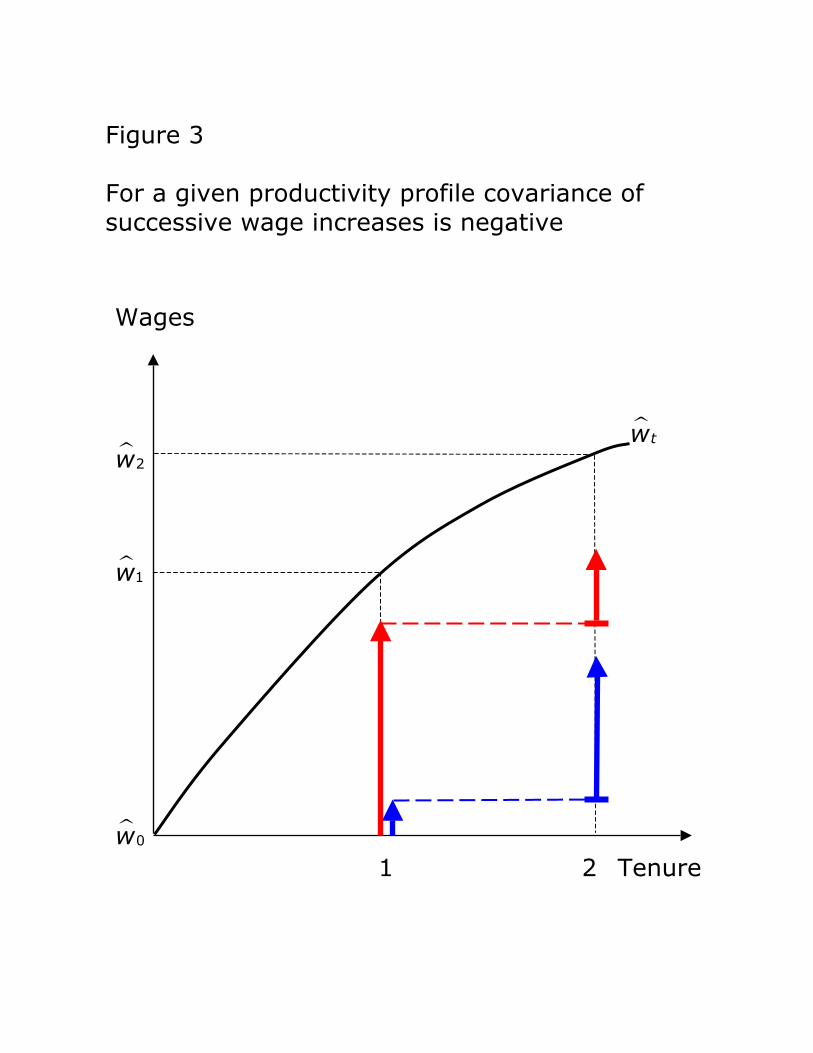
Figure 3 For a given productivity profile covariance of successive wage increases is negative

Wages

w

1

2

0

t

Tenure 1 2

w

w

w

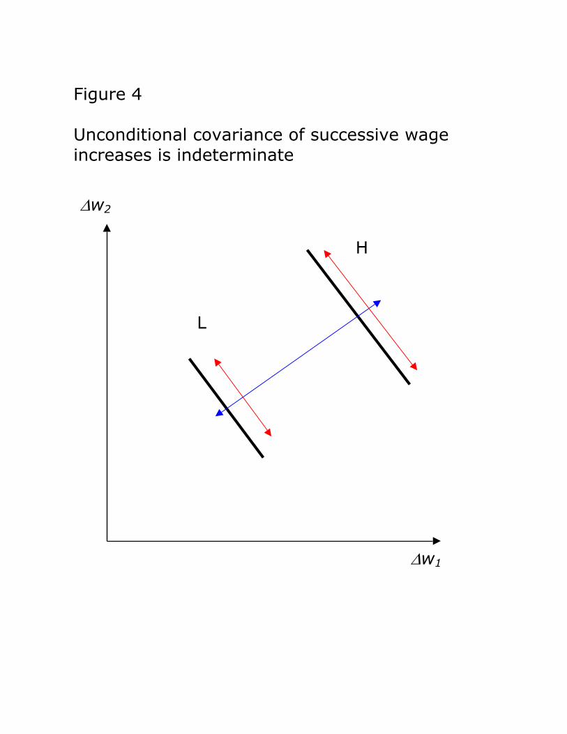
Figure 4 Unconditional covariance of successive wage increases is indeterminate

H

L

∆w1

∆w2