A Theory of the Budgetary ProcessAuthor(s): Otto A. Davis, M. A. H. Dempster and Aaron WildavskyReviewed work(s):Source: The American Political Science Review, Vol. 60, No. 3 (Sep., 1966), pp. 529-547Published by: American Political Science AssociationStable URL: http://www.jstor.org/stable/1952969 .Accessed: 31/07/2012 15:11

Your use of the JSTOR archive indicates your acceptance of the Terms & Conditions of Use, available at .http://www.jstor.org/page/info/about/policies/terms.jsp

.JSTOR is a not-for-profit service that helps scholars, researchers, and students discover, use, and build upon a wide range ofcontent in a trusted digital archive. We use information technology and tools to increase productivity and facilitate new formsof scholarship. For more information about JSTOR, please contact support@jstor.org.

.

American Political Science Association is collaborating with JSTOR to digitize, preserve and extend access toThe American Political Science Review.

http://www.jstor.org

The American

Political Science Review

VOL. LX SEPTEMBER, 1966 NO. 3

A THEORY OF THE BUDGETARY PROCESS*

OTTO A. DAVIS, M. A. H. DEMPSTER, AND AARON WILDAVSKY Carnegie Institute of Technology, Nuffield College, Oxford, and University of California, Berkeley

There are striking regularities in the bud- getary process. The evidence from over half of the non-defense agencies indicates that the be- havior of the budgetary process of the United States government results in aggregate deci- sions similar to those produced by a set of sim- ple decision rules that are linear and temporally stable. For the agencies considered, certain equations are specified and compared with data composed of agency requests (through the Bureau of the Budget) and Congressional ap- propriations from 1947 through 1963. The com- parison indicates that these equations sum- marize accurately aggregate outcomes of the budgetary process for each agency.

In the first section of the paper we present an analytic summary of the federal budgetary process, and we explain why basic features of the process lead us to believe that it can be rep- resented by simple models which are stable over periods of time, linear, and stochastic.' In the second section we propose and discuss the alternative specifications for the agency-Bud- get Bureau and Congressional decision equa- tions. The empirical results are presented in section three. In section four we provide evi-

* The research was sponsored by Resources for the Future. We received valuable criticism from Rufus Browning, Sam Cohn, W. W. Cooper, Richard Cyert, Nelson Polsby, Herbert Simon, and Oliver Williamson, research assistance from Rose Kelly, and editorial assistance from Jean Zorn. Mrs. E. Belton undertook the laborious task of compiling the raw data. We are grateful to Resources for the Future and to our colleagues, but the sole responsibility for what is said here is our own.

I See the Appendix for explanations of terms and concepts.

dence on deviant cases, discuss predictions, and future work to explore some of the problems indicated by this kind of analysis. An appendix contains informal definitions and a discussion of the statistical terminology used in the paper.

I. THE BUDGETARY PROCESS

Decisions depend upon calculation of which alternatives to consider and to choose.2 A major clue toward understanding budgeting is the extraordinary complexity of the calculations involved. There are a huge number of items to be considered, many of which are of consider- able technical difficulty. There is, however, little or no theory in most areas of policy which would enable practitioners to predict the con- sequences of alternative moves and the prob- ability of their occurring. Nor has anyone solved the imposing problem of the inter-per- sonal comparison of utilities. Outside of the political process, there is no agreed upon way of comparing and evaluating the merits of differ- ent programs for different people whose pre- ferences vary in kind and in intensity.

Participants in budgeting deal with their overwhelming burdens by adopting aids to calculation. By far the most important aid to calculation is the incremental method. Budgets are almost never actively reviewed as a whole in the sense of considering at once the value of all existing programs as compared to all possi- ble alternatives. Instead, this year's budget is

2 The description which follows is taken from Aaron Wildavsky, The Politics of the Budgetary Process (Boston, 1964). Portions of the comments on the House Appropriations Committee are from Richard Fenno, "The House Appropriations Committee as a Political System: The Problem of Integration," this REVIEW, 56 (1962), 310-324.

529

530 THE AMERICAN POLITICAL SCIENCE REVIEW

based on last year's budget, with special atten- tion given to a narrow range of increases or de- creases.

Incremental calculations proceed from an existing base. (By "base" we refer to common- ly held expectations among participants in budgeting that programs will be carried out at close to the going level of expenditures.) The widespread sharing of deeply held expectations concerning the organization's base provides a powerful (although informal) means of securing stability.

The most effective coordinating mechanisms in budgeting undoubtedly stem from the roles adopted by the major participants. Roles (the expectations of behavior attached to institu- tional positions) are parts of the division of labor. They are calculating mechanisms. In American national government, the adminis- trative agencies act as advocates of increased expenditure, the Bureau of the Budget acts as Presidential servant with a cutting bias, the House Appropriations Committee functions as a guardian of the Treasury, and the Senate Appropriations Committee as an appeals court to which agencies carry their disagreements with House action. The roles fit in with one an- other and set up patterns of mutual expecta- tions which markedly reduce the burden of calculation for the participants. Since the agencies can be depended upon to advance all the programs for which there is prospect of sup- port, the Budget Bureau and the Appropria- tions Committees respectively can concentrate on fitting them into the President's program or paring them down.

Possessing the greatest expertise and the largest numbers, working in the closest prox- imity to their policy problems and clientele groups, and desiring to expand their horizons, administrative agencies generate action through advocacy. But if they ask for amounts much larger than the appropriating bodies be- lieve reasonable, the agencies' credibility will suffer a drastic decline. In such circumstances, the reviewing organs are likely to cut deeply, with the result that the agency gets much less than it might have with a more moderate re- quest. So the first guide for decision is: do not come in too high. Yet the agencies must also not come in too low, for the reviewing bodies assume that if agency advocates do not ask for funds they do not need them. Thus, the agency decision rule might read: come in a little too high (padding), but not too high (loss of con- fidence).

Agencies engage in strategic planning to secure these budgetary goals. Strategies are the links between the goals of the agencies and their perceptions of the kinds of actions which

will be effective in their political environment. Budget officers in American national govern- ment uniformly believe that being a good poli- tician-cultivation of an active clientele, devel- opment of confidence by other officials (partic- ularly the appropriations subcommittees), and skill in following strategies which exploit op- portunities-is more important in obtaining funds than demonstration of agency efficiency.

In deciding how much money to recommend for specific purposes, the House Appropriations Committee breaks down into largely autono- mous subcommittees in which the norm of reciprocity is carefully followed. Specialization is carried further as subcommittee members develop limited areas of competence and juris- diction. Budgeting is both incremental and fragmented as the subcommittees deal with adjustments to the historical base of each agency. Fragmentation and specialization are increased through the appeals functions of the Senate Appropriations Committee, which deals with what has become (through House action) a fragment of a fragment. With so many partici- pants continually engaged in taking others into account, a great many adjustments are made in the light of what others are likely to do.

This qualitative account of the budgetary process contains clear indications of the kind of quantitative models we wish to develop. It is evident, for example, that decision-makers in the budgetary process think in terms of per- centages. Agencies talk of expanding their base by a certain percentage. The Bureau of the Budget is concerned about the growth rates for certain agencies and programs. The House Ap- propriations Committee deals with percentage cuts, and the Senate Appropriations Commit- tee with the question of whether or not to restore percentage cuts. These considerations suggest that the quantitative relationships among the decisions of the participants in the budget process are linear in form.

The attitudes and calculations of partici- pants in budgeting seem stable over time. The prominence of the agency's "base" is a sign of stability. The roles of the major participants are powerful, persistent, and strongly grounded in the expectations of others as well as in the internal requirements of the positions. Stabiltiy is also suggested by the specialization that occurs among the participants, the long service of committee members, the adoption of incre- mental practices such as comparisons with the previous year, the fragmentation of appropria- tions by program and item, the treatments of appropriations as continuously variable sums of money rather than as perpetual reconsidera- tions of the worth of programs, and the practice

A THEORY OF THE BUDGETARY PROCESS 531

of allowing past decisions to stand while coordi- nating decision-making only if difficulties arise. Since the budgetary process appears to be stable over periods of time, it is reasonable to estimate the relationships in budgeting on the basis of time series data.

Special events that upset the apparent sta- bility of the budgetary process can and do occur. Occasionally, world events take an un- expected turn, a new President occupies the White House, some agencies act with excep- tional zeal, others suffer drastic losses of con- fidence on the part of the appropriations sub- committees, and so on. It seems plausible to rep- resent such transient events as random shocks to an otherwise deterministic system. There- fore, our model is stochastic rather than deter- ministic.

The Politics of the Budgetary Process contains a description of strategies which various partic- ipants in budgeting use to further their aims. Some of these strategies are quite complicated. However, a large part of the process can be ex- plained by some of the simpler strategies which are based on the relationship between agency requests for funds (through the Budget Bu- reau) and Congressional appropriations. Be- cause these figures are made public and are known to all participants, because they are directly perceived and communicated without fear of information loss or bias, and because the participants react to these figures, they are ideal for feedback purposes. It is true that there are other indicators-special events, crises, technological developments, actions of clientele groups-which are attended to by participants in the budgetary process. But if these indi- cators have impact, they must quickly be re- flected in the formal feedback mechanisms- the actions of departments, the Bureau of the Budget, and Congress-to which they are di- rected. Some of these indicators (see section iv) are represented by the stochastic disturbances. Furthermore, the formal indicators are more precise, more simple, more available, more easily interpreted than the others. They are, therefore, likely to be used by participants in the budgetary process year in and year out. Present decisions are based largely on past ex- perience, and this lore is encapsulated in the amounts which the agencies receive as they go through the steps in the budgetary cycle.

For all the reasons discussed in this section, our models of the budgetary process are linear, stable over periods of time, stochastic, and strategic in character. They are "as if" models: an excellent fit for a given model means only that the actual behavior of the participants has an effect equivalent to the equations of the model. The models, taken as a whole, represent

a set of decision rules for Congress and the agencies.

II. THE MODELS

In our models we aggregate elements of the decision-making structure. The Budget Bureau submissions for the agency are used instead of separate figures for the two kinds of organiza- tions. Similarly, at this stage in our analysis, we use final Congressional appropriations instead of separating out committee action, floor ac- tion, conference committee recommendations, and so on. We wish to emphasize that although there may be some aggregation bias in the estimation of the postulated structure of deci- sion, this does not affect the linearity of the aggregate relationships. If the decisions of an agency and the Bureau of the Budget with re- gard to that agency depend linearly upon the same variable (as we hypothesize), then the aggregated decision rule of the two, treated as a single entity, will depend linearly upon that variable. By a similar argument, the various Congressional participants can be grouped to- gether so that Congress can be regarded as a single decision-making entity. While the aggre- gating procedure may result in grouping posi- tive and negative influences together, this manifestly does not affect the legitimacy of the procedure; linearity is maintained.3

Our models concern only the requests pre- sented in the President's budget for an individ- ual agency and the behavior of Congress as a whole with regard to the agency's appropria- tion. The models do not attempt to estimate the complete decision-making structure for each agency from bureau requests to depart- ments to submission through the Budget Bu- reau to possible final action in the Senate and House. There are several reasons for remaining content with the aggregated figures we use. First, the number of possible decision rules which must be considered grows rapidly as each new participant is added. We would soon be overwhelmed by the sheer number of rules invoked. Second, there are genuine restrictions placed on the number of structural parameters we can estimate because (a) some data, such as bureau requests to departments, are unavail- able, and (b) only short time series are mean- ingful for most agencies. It would make no sense, for example, to go back in time beyond the end of World War II when most domestic activity was disrupted.4

3 See H. Thiel, Linear Aggregation of Economic Relations (Amsterdam, 1954).

4 Our subsequent discussion of "shift" or "break" points should also make clear that it is

532 THE AMERICAN POLITICAL SCIENCE REVIEW

Since the agencies use various strategies and Congress may respond to them in various ways, we propose several alternative systems of equa- tions. These equations represent alternative decision rules which may be followed by Con- gressional and agency-Budget Bureau partici- pants in the budgetary process. One important piece of data for agency-Budget Bureau per- sonnel who are formulating appropriations re- quests is the most recent Congressional appro- priation. Thus, we make considerable use of the concept "base," operationally defined as the previous Congressional appropriation for an agency, in formulating our decision rules. Since the immediate past exercises such a heavy in- fluence on budgetary outcomes, Markov (si- multaneous, difference) equations are partic- ularly useful. In these Markov processes, the value of certain variables at one point in time is dependent on their value at one or more im- mediately previous periods as well as on the particular circumstances of the time.

We postulate several decision rules for both the agency-Budget Bureau requests and for Congressional action on these requests. For each series of requests or appropriations, we select from the postulated decision rules that rule which most closely represents the behavior of the aggregated entities. We use the variables

yt the appropriation passed by Congress for any given agency in the year t. Supple- mental appropriations are not included in the yt.

x: the appropriation requested by the Bureau of the Budget for any given agency for the year t. The xt constitutes the President's budget request for an agency.

We will also introduce certain symbols repre- senting random disturbances of each of the postulated relationships. These symbols are explained as they are introduced.

A. Equations for Agency-Budget Bureau Deci- sion Rules. The possibility that different agencies use different strategies makes it neces- sary to construct alternative equations repre- senting these various strategies. Then, for each agency in our sample, we use time series data to select that equation which seems to describe best the budgetary decisions of that agency. In this section we present three simple models of agency requests. The first states agency re- quests as a function of the previous year's ap- propriation. The second states requests as a function of the previous appropriation as well as a function of the differences between the

not realistic to expect meaningful time series of great length to be accumulated for most agencies in the United States government.

agency request and appropriation in the previ- ous year. The third states requests as a func- tion of the previous year's request. In all three linear models provision is made for a random variable to take into account the special cir- cumstances of the time.

An agency, while convinced of the worth of its programs, tends to be aware that extraor- dinarily large or small requests are likely to be viewed with suspicion by Congress; an agency does not consider it desirable to make extraor- dinary requests, which might precipitate un- favorable Congressional reaction. Therefore, the agency usually requests a precentage (gen- erally greater than one hundred percent) of its previous year's appropriation. This percentage is not fixed: in the event of favorable circum- stances, the request is a larger percentage of the previous year's appropriation than would otherwise be the case; similarly, the percentage might be reduced in the event of unfavorable circumstances.

Decisions made in the manner described above may be represented by a simple equa- tion. If we take the average of the percentages that are implicitly or explicitly used by budget officers, then any request can be represented by the sum of this average percentage of the previ- ous year's appropriation plus the increment or decrement due to the favorable or unfavorable circumstances. Thus

(1) ot = mYt-a + (t

The agency request (through the Budget Bureau) for a certain year is a fixed mean percentage of the Congressional appropria- tion for that agency in the previous year plus a random variable (normally distributed with mean zero and unknown but finite vari- ance) for that year.

is an equation representing this type of be- havior. The average or mean percentage is re- presented by fo. The increment or decrement due to circumstances is represented by ~t, a var- iable which requires some special explanation. It is difficult to predict what circumstances will occur at what time to put an agency in a favor- able or unfavorable position. Numerous events could influence Congress's (and the public's) perception of an agency and its programs-the occurrence of a destructive hurricane in the case of the Weather Bureau, the death by cancer of a friend of an influential congressman, in the case of the National Institutes of Health, the hiring (or losing) of an especially effective lobbyist by some interest group, the President's becoming especially interested in a program of some agency as Kennedy was in mental health, and so on. (Of course, some of them may be more or less "predictable" at certain times to an experienced observer, but this fact causes no

A THEORY OF THE BUDGETARY PROCESS 533

difficulty here.) Following common statistical practice we may represent the sum of the ef- fects of all such events by a random variable that is an increment or decrement to the usual percentage of the previous year's appropria- tion. In equation (1), then, it represents the value which this random variable assumes in year t.

We have chosen to view the special events of each year for each agency as random phenom- ena that are capable of being described by a probability density or distribution. We assume here that the random variable is normally dis- tributed with mean zero and an unknown but finite variance. Given this specification of the random variable, the agency makes its budget- ing decisions as if it were operating by the pos- tulated decision rule given by equation (1).

An agency, although operating somewhat like the organizations described by equation (1), may wish to take into account an addition- al strategic consideration: while this agency makes a request which is roughly a fixed per- centage of the previous year's appropriation, it also desires to smooth out its stream of appro- priations by taking into account the difference between its request and appropriation for the previous year. If there were an unusually large cut in the previous year's request, the agency submits a "padded" estimate to make up for the loss in expected funds; an unusual increase is followed by a reduced estimate to avoid un- spent appropriations. This behavior may be rep- resented by equation or decision rule where

(2) Xt = PlYt-1 + 132(yt-1 - Xf1) + xt

The agency request (through the Budget Bureau) for a certain year is a fixed mean percentage of the Congressional appropria- tion for that agency in the previous year plus a fixed mean percentage of the difference be- tween the Congressional appropriation and the agency request for the previous year plus a stochastic disturbance.

xt is a stochastic disturbance, which plays the role described for the random variable in equa- tion (1), the O's are variables reflecting the aspects of the previous year's request and ap- propriation that an agency takes into account: A3 represents the mean percentage of the previ- ous year's request which is taken into account, and O2 represents the mean percentage of the difference between the previous year's appro- priation and request (yt.,-xti) which is taken into account. Note that 12 <O is anticipated so that a large cut will (in the absence of the events represented by the stochastic distur- bance) be followed by a padded estimate and vice-versa.'

6 Since some readers may not be familiar with

Finally, an agency (or the President through the Bureau of the Budget), convinced of the worth of its programs, may decide to make re- quests without regard to previous Congression- al action. This strategy appeals especially when Congress has so much confidence in the agency that it tends to give an appropriation which is almost identical to the request. Aside from special circumstances represented by stochastic disturbances, the agency's request in any given year tends to be approximately a fixed percent- age of its request for the previous year. This behavior may be represented by

(3) Xt = l3Xt-i + Pt

The agency request (through the Budget Bureau) for a certain year is a fixed mean percentage of the agency's request for the previous year plus a random variable (sto- chastic disturbance).

where pt is a stochastic disturbance and p is

the average percentage. Note that if the agency believes its programs to be worthy, /3 >1 is expected.'

These three equations are not the only ones which may be capable of representing the ac- tual behavior of the combined budgeting deci- sions of the agencies and the Bureau of the Budget. However, they represent the agency-

the notation we are using, a brief explanation may be in order. As a coefficient of the equation, 32 is an unknown number that must be estimated from the data, and this coefficient multiplies another number (yt-1 -xt-1) that may be computed by subtracting last year's request from last year's appropriation. We want the equation to say that the agency will try to counteract large changes in their appropriations by changing their normal requests in the next year. If the agency asks for much more than it thinks it will get and its request is cut, for example, the expression (Yt- -Xti1) will be a negative number written in symbolic form as (yti -xt-1) <0. A rule of multi- plication says that a negative number multiplied by another negative number gives a positive num- ber. If an agency pads its request, however, it presumably follows a cut with a new request which incorporates an additional amount to make allowance for future cuts. In order to represent this behavior, that is to come out with a positive result incorporating the concept of padding, the unknown coefficient 2 must be negative (02 <0)-

6 The agency that favors its own programs should increase its requests over time. In the absence of the stochastic disturbance (when the random variable is 0), the request in a given year should be larger than the request in the previous year so that xe >xg_. Therefore, the unknown coefficient /3 must be larger than one (/3 > 1) since

it multiplies last year's request.

534 THE AMERICAN POLITICAL SCIENCE REVIEW

Budget Bureau budgeting behavior better than all other decision rules we tried.7

B. Equations for Congressional Decision Rules. In considering Congressional behavior, we again postulate three decision equations from which a selection must be made that best represents the behavior of Congress in regard to an agency's appropriations. Since Congress may use various strategies in determining ap- propriations for different agencies, different Congressional decision equations may be selected as best representing Congressional ap- propriations for each agency in our sample. Our first model states Congressional appropria- tions as a function of the agency's request (through the Budget Bureau) to Congress. The second states appropriations as a function of the agency's request as well as a function of

I Other gaming strategies are easily proposed. Suppose, for example, that a given agency be- lieves that it knows the decision rule that Con- gress uses in dealing with it, and that this decision rule can be represented by one of (4), (7), or (8), above. Presume, for reasons analogous to those outlined for (8), that this agency desires to take into account that positive or negative portion of the previous year's appropriation Ye-i that was not based on the previous year's request xt-. This consideration suggests

Xt = I4yt-1 + I5At-1 + St

as an agency decision rule where At-, is a dummy variable representing in year t - 1 the term not involving xtei in one of (4), (7) or (8) above. If one believes that agency and Bureau of the Budget personnel are sufficiently well acquainted with the senators and congressmen to be able to predict the value of the current stochastic disturbance, then it becomes reasonable to examine a decision rule of the form

Xt = I6yt-I + 07A9 + ot

where At is defined as above. No evidence of either form of behavior was found, however, among the agencies that were investigated. We also esti- mated the parameters of the third order auto- regressive scheme for the requests of an individual agency

Xt = l8Xt-I + f9Xte2 + IjiXt_-3 + Tt

in an attempt to discover if naive models would fit as well as those above. In no case did this occur and generally the fits for this model were very poor. A similar scheme was estimated for the appropriations ye of an individual agency with similar results with respect to qeuations (4), (7) and (8) above. Since the "d" statistic suggests that no higher order Markov process would be successful, no other rules for agency behavior were tried.

the deviation from the usual relationship be- tween Congress and the agency in the previous year. The third model states appropriations as a function of that segment of the agency's re- quest that is not part of its appropriation or re- quest for the previous year. Random variables are included to take account of special circum- stances.

If Congress believes that an agency's re- quest, after passing through the hands of the Budget Bureau, is a relatively stable index of the funds needed by the agency to carry out its programs, Congress responds by appropriating a relatively fixed percentage of the agency's re- quest. The term "relatively fixed" is used be- cause Congress is likely to alter this percentage somewhat from year to year because of special events and circumstances relevant to particular years. As in the case of agency requests, these special circumstances may be viewed as random phenomena. One can view this behavior as if it were the result of Congress' appropriating a fixed mean percentage of the agency requests; adding to the amount so derived a sum repre- sented by a random variable. One may repre- sent this behavior as if Congress were following the decision rule

(4) yt = aoxt + qt The Congressional appropriation for an agency in a certain year is a fixed mean per- centage of the agency's request in that year plus a stochastic disturbance.

where ao represents the fixed average percen- tage and nt represents the stochastic distur- bance.

Although Congress usually grants an agency a fixed percentage of its request, this request sometimes represents an extension of the agency's programs above (or below) the size desired by Congress. This can occur when the agency and the Bureau of the Budget follow Presidential aims differing from those of Con- gress, or when Congress suspects that the agency is padding the current year's request. In such a situation Congress usually appropriates a sum different from the usual percentage. If a, represents the mean of the usual percentages, this behavior can be represented by equation or decision rule

(5) ys = aixt + vt

where vt is a stochastic disturbance represent- ing that part of the appropriations attributable to the special circumstances that cause Con- gress to deviate from a relatively fixed percent- age. Therefore, when agency aims and Con- gressional desires markedly differ from usual (so that Congress may be said to depart from its usual rule) the stochastic disturbance takes on an unusually large positive or negative

A THEORY OF THE BUDGETARY PROCESS 535

value. In order to distingush this case from the previous one, more must be specified about the stochastic disturbance vt. In a year following one in which agency aims and Congressional desires markedly differed, the agency makes a request closer to Congressional desires, and/or Congress shifts its desires closer to those of the agency (or the President). In the year after a deviation, then, assume that Congress will tend to make allowances to normalize the situation. Such behavior can be represented by having the stochastic disturbance vt generated in ac- cordance with a first order Markov scheme. The stochastic component in vt is itself deter- mined by a relation (6) vt = a2vf.l + eg

where et is a random variable. The symbol vt therefore stands for the stochastic disturbance in the previous year (vt-i) as well as the new stochastic disturbance for the year involved (et). Substituting (6) into (5) gives (7) yt = aixt + a2Vt-I + Et

The Congressional appropriation for an agency is a fixed mean percentage of the agency's request for that year plus a sto- chastic disturbance representing a deviation from the usual relationship between Congress and the agency in the previous year plus a random variable for the current year.

as a complete description of a second Congress- ional decision rule. If Congress never makes complete allowance for an initial '"deviation," then -1 <a2<1 is to be expected.

To complete the description of this second Congressional decision rule, we will suppose 0 <a2<1. Then, granted a deviation from its usual percentage, Congress tends to decrease subsequent deviations by moving steadily back toward its usual percentage (except for the un- foreseeable events or special circumstances whose effects are represented by the random variable Et). For example, if in a particular year vt-1 >0, and if in the following year there are no special circumstances so that it = 0, then vt=a2Vt-l <vti,. The deviation in year t is smaller than the deviation in year t-1. How- ever, if -1 <a2<0. after an initial deviation, Congress tends to move back to its usual rule (apart from the disturbances represented by the random variable Et) by making successively smaller deviations which differ in sign. For ex- ample, if vt-1 >0, then apart from the distur- bance et it is clear that vt = a2vt-1 <0, since a2 <0. Finally, if a2= 0, decision rule (7) is the same as the previous rule (4).

The specialization inherent in the appropria- tions process allows some members of Congress to have an intimate knowledge of the budget- ary processes of the agencies and the Budget Bureau. Thus, Congress might consider that

part of the agency's request (xt) which is not based on the previous year's appropriation or request. This occurs when Congress believes that this positive or negative remainder repre- sents padding or when it desires to smooth out the agency's rate of growth. If Congress knows the decision rule that an agency uses to formu- late its budgetary request, we can let Xt repre- sent a dummy variable defined as Xt = t if the agency uses decision rule (1); Xt=f2(Yt-1 - Xt-) +Xt if the agency uses decision rule (2); and, Xt =pt if the agency uses decision rule (3). Suppose that Congress appropriates, on the average, an amount which is a relatively fixed percentage of the agency's request plus a per- centage of this (positive or negative) remainder Xt. This behavior can be represented by the "as if" decision rule

(8) yt = a3xt + a4Xt + Vt The Congressional appropriation for an agency is a fixed mean percentage of the agency's request for a certain year plus a fixed mean percentage of a dummy variable which represents that part of the agency's re- quest for the year at issue which is not part of the appropriation or request of the previ- ous year plus a random variable representing the part of the appropriation attributable to the special circumstances of the year.

where vt is a stochastic disturbance whose value in any particular year represents the part of the appropriation attributable to the agency's special circumstances of the year. One might expect that Congress takes only "partial" ac- count of the remainder represented by Xt, SO 0 <a4<1.

III. EMPIRICAL RESULTS

Times series data for the period 1947-1963 were studied for fifty-six non-defense agencies of the United States Government. The requests (xt) of these agencies were taken to be the amounts presented to Congress in the Presi- dent's budget. For eight sub-agencies from the National Institutes of Health, data for a shorter period of time were considered, and the requests (xt) of these eight sub-agencies were taken to be their proposals to the Bureau of the Budget.8 In all instances the Congressional de- cision variable (ye) was taken to be the final ap- propriation before any supplemental additions. The total appropriations (without supple- ments) of the agencies studied amounted to approximately twenty-seven percent of the non-defense budget in 1963. Over one-half of all non-defense agencies were investigated; the major omissions being the Post Office and many independent agencies. A minimum of three

8 Agency proposals to the Bureau of the Budget are not reported to the public and could be ob- tained only for these eight sub-agencies.

536 THE AMERICAN POLITICAL SCIENCE REVIEW

agencies was examined from each of the Trea- sury, Justice, Interior, Agriculture, Commerce, Labor, and Health, Education and Welfare Departments.9

If the agency-Budget Bureau disturbance is independent of Congressional disturbances the use of ordinary least squares (OLS) to esti- mate most of the possible combinations of the proposed decision equations is justified. OLS is identical to the simultaneous full information maximum likelihood (FIML) technique for most of the present systems. This is not so, however, for some systems of equations be- cause of the presence of an auto-correlated dis- turbance in one equation of the two and the consequent non-linearity of the estimating equations. In equation (6) the stochastic dis- turbance for year t is a function of the value of the disturbance in the previous year. In a sys- tem of equations in which auto-correlation occurs in the first equation, an appropriate

9 Three interrelated difficulties arise in the analysis of the time series data xt, ye for an agency. The first problem is the choice of a technique for estimating the parameters of the alternate schemes in some optimal fashion. Given these estimates and their associated statistics, the sec- ond problem is the choice of criteria for selecting the model best specifying the system underlying the data. Finally, one is faced with the problem of examining the variability of the underlying pa- rameters of the best specification. We believe that our solution to these problems, while far from optimal, is satisfactory given the present state of econometric knowledge. See our presentation in "On the Process of Budgeting: An Empirical Study of Congressional Appropriations," by Otto Davis, M. A. H. Dempster, and Aaron Wildavsky, to appear in Gordon Tullock (ed.), Papers on Non-Market Decision Making, Thomas Jefferson Center, University of Virginia. See especially section 4 and the appendix by Demp- ster, which contains discussions and derivations of estimation procedures, selection criteria and test statistics for the processes in Section II of this paper.

10 We make the assumption that these two disturbances are independent throughout the paper. Notice, however, that dependence between the disturbances explicitly enters decision equa- tion (8) of section II and those of footnote 7. For these equations, the assumption refers to the disturbance of the current year. That is, we allow the possibility that special circumstances may affect a single participant (Bureau of the Budget or Congress) as well as both. When the latter case occurred, our selection criteria resulted in the choice of equation (8) as best specifying Congres- sional behavior.

procedure is to use OLS to estimate the alter- native proposals for the other equation, decide by the selection criteria which best specifies the data, use the knowledge of this structure to estimate the first equation, and then decide, through use of appropriate criteria, which ver- sion of the first equation best specifies the data.

The principal selection criterion we used is that of maximum (adjusted) correlation coefficient (R). For a given dependent variable this criterion leads one to select from alterna- tive specifications of the explanatory variables, that specification which leads to the highest sample correlation coefficient. The estimations of the alternative specifications must, of course, be made from the same data." The second criterion involves the use of the d-statistic test for serial correlation of the estimated residuals of a single equation.'2 This statistic tests the null hypothesis of residual independence against the alternative of serial correlation. We used the significance points for the d-statistic of Theil and Nagar.'3 When the d-statistic was found to be significant in fitting the Congres- sional decision equation (4) to an agency's data, it was always found that equation (7) best spec- ified Congressional behavior with respect to the appropriations of that agency in the sense of yielding the maximum correlation coeffi- cient. A third criterion is based on a test of the significance of the sample correlation between the residuals of (4) and the estimated Xt of the equation selected previously for a given agency. David's significance points for this statistic were used to make a two-tailed test at the five percent level of the null hypothesis that the residuals are uncorrelated.'4 When significant

11 We are estimating the unknown values of the coefficients (or parameters) of regression equa- tions for each agency. All of our estimators are biased. We use biased estimators for the simple reason that no unbiased estimators are known. The property of consistency is at least a small comfort. All of our estimators are consistent. It might be noted that all unbiased estimators are consistent, but not all consistent estimators are unbiased.

12 This statistic is known as the Durbin-Watson ratio. A description of the test may be found in J. Johnston, Econometric Methods (New York, 1963), p. 92.

13 H. Theil and A. L. Nagar, "Testing the Inde- pendence of Regressional Disturbances," Journal of the American Statistical Association, 56 (1961), 793-806. These significance points were used to construct further significance points when neces- sary. See Davis, Dempster and Wildavsky, op. cit.

14 The test is described in T. W. Anderson, An Introduction to Multivariate Analysis (New York,

A THEORY OF THE BUDGETARY PROCESS 537

TABLE 1. BEST SPECIFICATIONS FOR EACH AGENCY ARE HIGH

Frequencies of Correlation Coefficients

1 -.995- .99- .98- .97- .96- .95- .94- .93 - .90- .85- 0

Congressional 21 8 15 4 5 2 2 1 5 2 2

Agency-Bureau 9 2 2 8 5 2 4 3 5 11 10

correlation occurred, it was always found that Congressional decision equation (8), in which a function of the deviation from the usual re- lationship between request and the previous year's appropriation enters explicitly, best specified appropriation behavior with respect to the agency in question.

The statistical procedures were programmed for the Carnegie Institute of Technology's Control Data G-21 electronic computer in the 20-Gate algebraic compiling language. The selection among alternate specifications accord- ing to the criteria established was not done automatically; otherwise all computations were performed by machine. Since the results for each agency are described in detail else- where,15 and a full rendition would double the length of the paper, we must restrict ourselves to summary statements.

The empirical results support the hypothesis that, up to a random error of reasonable magni- tude, the budgetary process of the United States government is equivalent to a set of temporally stable linear decision rules. Esti- mated correlation coefficients for the best specifications of each agency are generally high. Although the calculated values of the multiple correlation coefficients (R's) tend to run higher in time series than in cross-sectional analysis, the results are good. We leave little of the variance statistically unexplained. More- over the estimated standard deviations of the coefficients are usually, much smaller than one- half of the size of the estimated coefficients, a related indication of good results. Table 1 pre- sents the frequencies of the correlation co- efficier ts.

The fits between the decision rules and the time series data for the Congressional decision equations are, in general, better than those for the agency-Bureau of the Budget equations. Of the 64 agencies and sub-agencies studied, there are only 14 instances in which the corre- lation coefficient for the agency (or sub-agency) equation was higher than the one for the corre-

1958) pp. 69-71. See Dempster's appendix to Davis, Dempster, and Wildavsky, op. cit., for some justification of the use of the test.

16 See Davis, Dempster, and Wildavsky, op. cit.

sponding Congressional equation. We specu- late that the estimated variances of the dis- turbances of the agency-Budget Bureau decision rules are usually larger because the agencies are closer than Congress to the actual sources that seek to add new programs or ex- pand old ones.

Table 2 presents a summary of the combina- tions of the Agency-Bureau of the Budget and Congressional decision equations. For those agencies studied, the most popular combina- tions of behavior are the simple ones repre- sented by equations (4) and (1) respectively. When Congress uses a sophisticated "gaming" strategy such as (7) or (8), the corresponding agency-Bureau of the Budget decision equation is the relatively simple (1). And, when Con- gress grants exactly or almost exactly the amount requested by an agency, the agency tends to use decision equation (3).

Our discussion thus far has assumed fixed values for the coefficients (parameters) of the equations we are using to explain the behavior underlying the budgetary process. In the light of the many important events occurring in the period from 1946 to 1963, however, it seems reasonable to suppose that the appropriations structure of many government agencies was altered. If this is correct, the coefficients of the equations-literally, in this context, the values represented by the on-the-average percentages requested by the agencies and granted by Congress-should change from one period of time to the next. The equations would then be temporally stable for a period, but not forever.

TABLE 2. BUDGETARY BEHAVIOR IS SIMPLE

Summary of Decision Equations

Agency-Budget Bureau 1 2 3

4 44* 1 8

Congress 7 1 0 0

8 12 0 's

* including eight sub-agencies from the National Institutes of Health

538 THE AMERICAN POLITICAL SCIENCE REVIEW

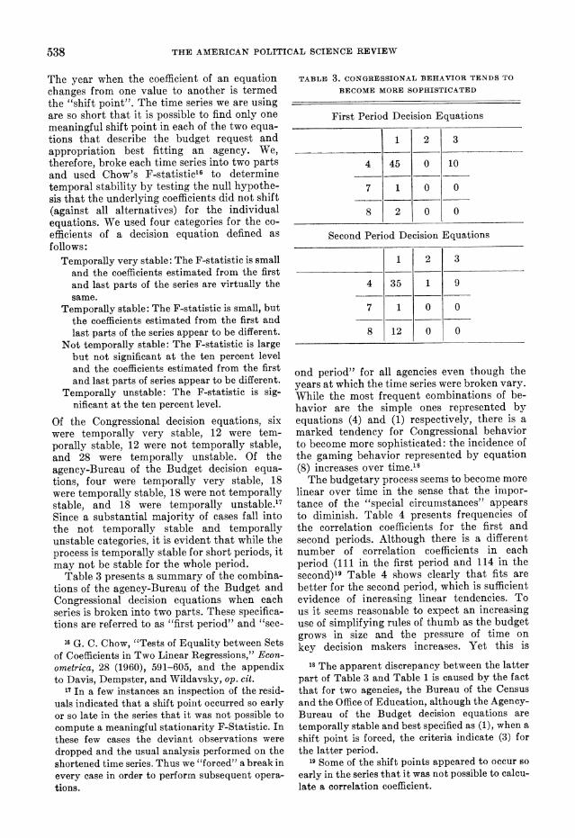
The year when the coefficient of an equation changes from one value to another is termed the "shift point". The time series we are using are so short that it is possible to find only one meaningful shift point in each of the two equa- tions that describe the budget request and appropriation best fitting an agency. We, therefore, broke each time series into two parts and used Chow's F-statistic'6 to determine temporal stability by testing the null hypothe- sis that the underlying coefficients did not shift (against all alternatives) for the individual equations. We used four categories for the co- efficients of a decision equation defined as follows:

Temporally very stable: The F-statistic is small and the coefficients estimated from the first and last parts of the series are virtually the same.

Temporally stable: The F-statistic is small, but the coefficients estimated from the first and last parts of the series appear to be different.

Not temporally stable: The F-statistic is large but not significant at the ten percent level and the coefficients estimated from the first and last parts of series appear to be different.

Temporally unstable: The F-statistic is sig- nificant at the ten percent level.

Of the Congressional decision equations, six were temporally very stable, 12 were tem- porally stable, 12 were not temporally stable, and 28 were temporally unstable. Of the agency-Bureau of the Budget decision equa- tions, four were temporally very stable, 18 were temporally stable, 18 were not temporally stable, and 18 were temporally unstable.'7 Since a substantial majority of cases fall into the not temporally stable and temporally unstable categories, it is evident that while the process is temporally stable for short periods, it may not be stable for the whole period.

Table 3 presents a summary of the combina- tions of the agency-Bureau of the Budget and Congressional decision equations when each series is broken into two parts. These specifica- tions are referred to as "first period" and "sec-

16 G. C. Chow, "Tests of Equality between Sets of Coefficients in Two Linear Regressions," Econ- ometrica, 28 (1960), 591-605, and the appendix to Davis, Dempster, and Wildavsky, op. cit.

17 In a few instances an inspection of the resid- uals indicated that a shift point occurred so early or so late in the series that it was not possible to compute a meaningful stationarity F-Statistic. In these few cases the deviant observations were dropped and the usual analysis performed on the shortened time series. Thus we "forced" a break in every case in order to perform subsequent opera- tions.

TABLE 3. CONGRESSIONAL BEHAVIOR TENDS TO

BECOME MORE SOPHISTICATED

First Period Decision Equations

1 2 3

4 45 0 10

7 1 0 0

8 2 0 0

Second Period Decision Equations

1 2 3

4 35 1 9

7 1 0 0

8 12 0 0

ond period" for all agencies even though the years at which the time series were broken vary. While the most frequent combinations of be- havior are the simple ones represented by equations (4) and (1) respectively, there is a marked tendency for Congressional behavior to become more sophisticated: the incidence of the gaming behavior represented by equation (8) increases over time.'8

The budgetary process seems to become more linear over time in the sense that the impor- tance of the "special circumstances" appears to diminish. Table 4 presents frequencies of the correlation coefficients for the first and second periods. Although there is a different number of correlation coefficients in each period (111 in the first period and 114 in the second)'9 Table 4 shows clearly that fits are better for the second period, which is sufficient evidence of increasing linear tendencies. To us it seems reasonable to expect an increasing use of simplifying rules of thumb as the budget grows in size and the pressure of time on key decision makers increases. Yet this is

18 The apparent discrepancy between the latter part of Table 3 and Table 1 is caused by the fact that for two agencies, the Bureau of the Census and the Office of Education, although the Agency- Bureau of the Budget decision equations are

temporally stable and best specified as (1), when a

shift point is forced, the criteria indicate (3) for

the latter period. 19 Some of the shift points appeared to occur so

early in the series that it was not possible to calcu- late a correlation coefficient.

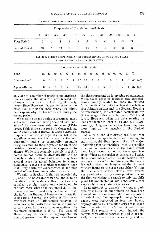
A THEORY OF THE BUDGETARY PROCESS 539

TABLE 4. THE BUDGETARY PROCESS IS BECOMING MORE LINEAR

Frequencies of Correlation Coefficients

1 -.995- .99 - .98- .97 - .96 - .94- .92 - .90 - .80 - .60 - 0

First Period 9 5 8 5 3 6 8 4 18 24 21

Second Period 27 5 13 8 8 15 7 5 12 8 6

TABLE 5. LIKELY SHIFT POINTS ARE CONCENTRATED IN THE FIRST YEARS

OF THE EISENHOWER ADMINISTRATION

Frequencies of Shift Points

Year 48 49 50 51 52 53 54 55 56 57 58 59 60 61 62 T

Congressional 0 2 3 1 0 1 17 16 1 1 3 0 0 1 0 46 (40)

Agency-Bureau 0 2 4 0 2 3 15 13 3 0 2 1 0 2 1 37 (36)

only one of a number of possible explanations. For example, the data are not deflated for changes in the price level during the early years. Since there were larger increases in the price level during the early years, this might help explain why the fits are better during the second period.

When only one shift point is presumed, most shifts are discovered during the first two bud- gets of the Eisenhower Administration (1954- 1955). Table 5 presents, for both Congressional and Agency-Budget Bureau decision equations, frequencies of the shift points for (a) those equations whose coefficients are in the not temporally stable or temporally un-stable categories and (b) those agencies for which the decision rules of the participants appeared to change. While it is certainly possible that shift points do not occur as dramatically and as sharply as shown here, and that it may take several years for actual behavior to change noticeably, Table 5 nevertheless makes it clear that likely shifts are concentrated in the first period of the Eisenhower administration.

We said, in Section II, that we expected i,, Al, and 13, to be greater than one, and 12 to be negative. In 56 instances this expectation is satisfied, but eight exceptions were noted. In the two cases where the estimated /3< 1, ex- planations are immediately available. First, the fit for the Bureau of Employment Security is not good. Second, the Office of Territories evidences most un-Parkinsonian behavior: its activities decline with a decrease in the number of territories. In the six other exceptions, the estimated coefficient is d3 <1. For three of these, Congress tends to appropriate an amount greater than the request, and two of

the three represent an interesting phenomenon. When those parts of requests and appropri- ations directly related to loans are omitted from the data for both the Rural Electrifica- tion Administration and the Federal Housing Administration, the estimated coefficients are of the magnitudes expected with fo > and a0 < 1. However, when the data relating to loans are included, then I3o < 1 and ao > 1. Ap- parently, Congress favors the loan programs more than do the agencies or the Budget Bureau.

As a rule, the d-statistics resulting from fitting the best specifications were not signifi- cant. It would thus appear that all major underlying trended variables (with the possible exception of variables with the same trend) have been accounted for by these specifica- tions. When an exception to this rule did exist, the authors made a careful examination of the residuals in an effort to determine the reason for such a situation. It appeared that in most of these instances the cause was either (a) that the coefficients shifted slowly over several years and not abruptly at one point in time, or (b) that restricting the search to only one shift point left undetected an additional shift either very early or very late in the series.

In an attempt to unmask the trended vari- able most likely (in our opinion) to have been ignored, and to cast some light upon the notion of "fair share," final appropriations yt for each agency were regressed on total non-defense appropriations zt. This time series was taken from the Statistical Abstract of the United States. The results were poor. Indeed, the sample correlations between yt and zt are us- ually worse than those between ye and xt.

540 THE AMERICAN POLITICAL SCIENCE REVIEW

Moreover, the d-statistics are usually highly significant and the residual patterns for the regression show the agency's proportion of the non-defense budget to be either increasing or decreasing over time. However, it should be noted that even those exceptional cases where the agency trend is close to that of the total non-defense appropriation do not invalidate the explicit decision structure fitted here. A similar study, with similar results, was con- ducted at the departmental level by regressing yt for the eight National Institutes of Health on yt for the Public Health Service, the agency of which they are a part. Finally, the yt for selected pairs of agencies with "similar" in- terests were regressed on each other with uni- formly poor results.

Although empirical evidence indicates that our models describe the budgetary process of the United States government, we are well aware of certain deficiencies in our work. One deficiency, omission of certain agencies from the study, is not serious because over one-half of all non-defense agencies were investigated. Nevertheless, the omission of certain agencies may have left undiscovered examples of ad- ditional decision rules. We will shortly study all agencies whose organizational structure can be traced. We will also include supplemental appropriations.

A more serious deficiency may lie in the fact that the sample sizes, of necessity, are small. The selection criterion of maximum sample cor- relation, therefore, lacks proper justification, and is only acceptable because of the lack of a better criterion. Further, full-information max- imum likelihood estimators, and especially biased ones, even when they are known to be consistent, are not fully satisfactory in such a situation, although they may be the best available. However, the remedy for these deficiencies must await the results of future theoretical research on explosive or evolu- tionary processes.

IV. THE DEVIANT CASES AND PREDICTION:

INTERPRETATION OF THE STOCHASTIC

DISTURBANCES

The intent of this section is to clarify further the interpretation of the stochastic distur- bances as special or unusual circumstances rep- resented by random variables. While those in- fluences present at a constant level during the period serve only to affect the magnitude of the coefficients, the special circumstances have an important, if subsidiary, place in these models. We have indicated that although outside ob- servers can view the effects of special circum- stances as a random variable, anyone familiar with all the facts available to the decision-

makers at the time would be able to explain the special circumstances. It seems reasonable therefore to examine instances where, in esti- mating the coefficients, we find that the esti- mated values of the stochastic disturbances assume a large positive or negative value. Such instances appear as deviant cases in the sense that Congress or the agency-Budget Bureau actors affected by special circumstances (large positive or negative values of the random variable) do not appear to be closely following their usual decision rule at that time but base their decisions mostly on these circumstances. The use of case studies for the analyses of deviant phenomena, of course, presupposes our ability to explain most budgeting decisions by our original formulations. Deviant cases, then, are those instances in which particular decisions do not follow our equations. It is possible to determine these deviant instances simply by examining the residuals of the fitted equations: one observes a plot of the residuals, selects those which appear as extreme positive or nega- tive values, determines the year to which these extreme residuals refer, and then examines evidence in the form of testimony at the Ap- propriations Committees, newspaper accounts and other sources. In this way it is possible to determine at least some of the circumstances of a budgetary decision and to investigate whether or not the use of the random variables is appropriate.20

Finally, it should be pointed out that in our model the occurrence of extreme disturbances represents deviant cas3s, or the temporary setting aside of their usual decision rules by the decision-makers in the process, while coefficient shifts represent a change (not necessarily in form) of these rules.

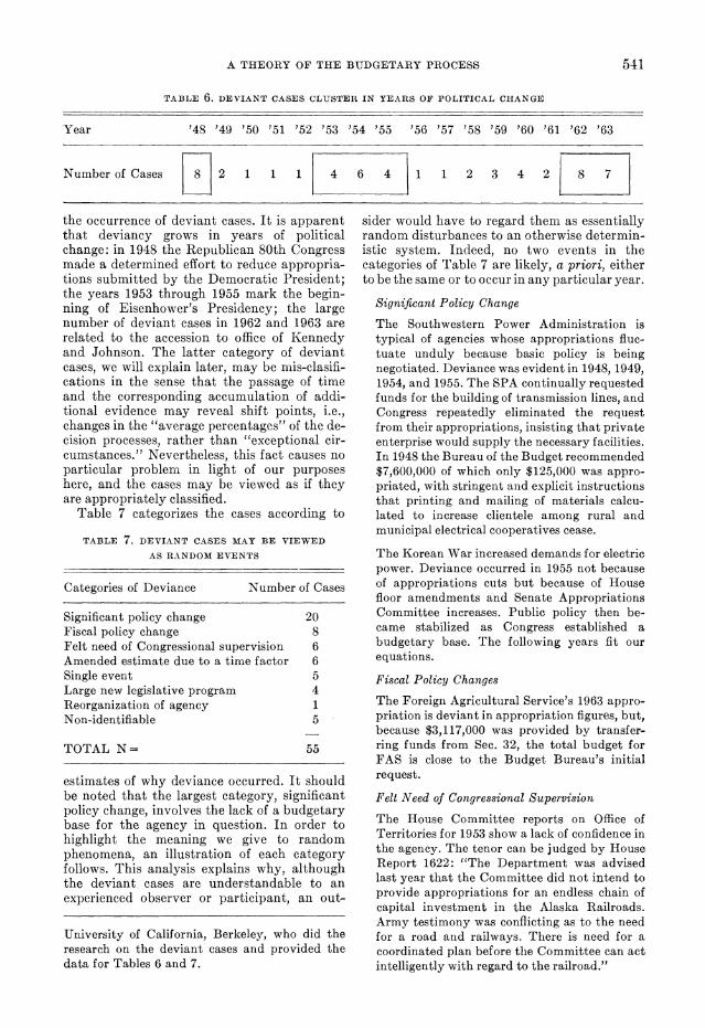
From the residuals of one-half of the esti- mated Congressional decision equations, a selection of 55 instances (approximately 14 percent of the 395 Congressional decisions under consideration) were identified as devi- ant.2' Table 6 shows the yearly frequency of

20 The importance of analyzing deviant cases is suggested in: Milton M. Gordon, "Sociological Law and the Deviant Case," Sociometry, 10 (1947); Patricia Kendall and Katharine Wolf, "The Two Purposes of Deviant Case Analysis," in Paul F. Lazarsfeld and Morris Rosenberg (eds.), The Language of Social Research, (Glencoe, 1962), pp. 103-137; Paul Horst, The Prediction of Per- sonal Adjustment: A Survey of the Logical Problems and Research Techniques (New York, 1941); and Seymour Lipset, Martin Trow, and James Cole- man, Union Democracy (New York, 1960).

21 We are indebted to Rose M. Kelly, a graduate student in the Department of Political Science,

A THEORY OF THE BUDGETARY PROCESS 541

TABLE 6. DEVIANT CASES CLUSTER IN YEARS OF POLITICAL CHANGE

Year '48 '49 '50 '51 '52 '53 '54 '55 '56 '57 '58 '59 '60 '61 '62 '63

Number of Cases 8 2 1 1 1 4 6 4 1 1 2 3 4 2 87

the occurrence of deviant cases. It is apparent that deviancy grows in years of political change: in 1948 the Republican 80th Congress made a determined effort to reduce appropria- tions submitted by the Democratic President; the years 1953 through 1955 mark the begin- ning of Eisenhower's Presidency; the large number of deviant cases in 1962 and 1963 are related to the accession to office of Kennedy and Johnson. The latter category of deviant cases, we will explain later, may be mis-clasifi- cations in the sense that the passage of time and the corresponding accumulation of addi- tional evidence may reveal shift points, i.e., changes in the "average percentages" of the de- cision processes, rather than "exceptional cir- cumstances." Nevertheless, this fact causes no particular problem in light of our purposes here, and the cases may be viewed as if they are appropriately classified.

Table 7 categorizes the cases according to

TABLE 7. DEVIANT CASES MAY BE VIEWED

AS RANDOM EVENTS

Categories of Deviance Number of Cases

Significant policy change 20 Fiscal policy change 8 Felt need of Congressional supervision 6 Amended estimate due to a time factor 6 Single event 5 Large new legislative program 4 Reorganization of agency 1 Non-identifiable 5

TOTAL N= 55

estimates of why deviance occurred. It should be noted that the largest category, significant policy change, involves the lack of a budgetary base for the agency in question. In order to highlight the meaning we give to random phenomena, an illustration of each category follows. This analysis explains why, although the deviant cases are understandable to an experienced observer or participant, an out-

University of California, Berkeley, who did the research on the deviant cases and provided the data for Tables 6 and 7.

sider would have to regard them as essentially random disturbances to an otherwise determin- istic system. Indeed, no two events in the categories of Table 7 are likely, a priori, either to be the same or to occur in any particular year.

Significant Policy Change

The Southwestern Power Administration is typical of agencies whose appropriations fluc- tuate unduly because basic policy is being negotiated. Deviance was evident in 1948, 1949, 1954, and 1955. The SPA continually requested funds for the building of transmission lines, and Congress repeatedly eliminated the request from their appropriations, insisting that private enterprise would supply the necessary facilities. In 1948 the Bureau of the Budget recommended $7,600,000 of which only $125,000 was appro- priated, with stringent and explicit instructions that printing and mailing of materials calcu- lated to increase clientele among rural and municipal electrical cooperatives cease.

The Korean War increased demands for electric power. Deviance occurred in 1955 not because of appropriations cuts but because of House floor amendments and Senate Appropriations Committee increases. Public policy then be- came stabilized as Congress established a budgetary base. The following years fit our equations.

Fiscal Policy Changes

The Foreign Agricultural Service's 1963 appro- priation is deviant in appropriation figures, but, because $3,117,000 was provided by transfer- ring funds from Sec. 32, the total budget for FAS is close to the Budget Bureau's initial request.

Felt Need of Congressional Supervision

The House Committee reports on Office of Territories for 1953 show a lack of confidence in the agency. The tenor can be judged by House Report 1622: "The Department was advised last year that the Committee did not intend to provide appropriations for an endless chain of capital investment in the Alaska Railroads. Army testimony was conflicting as to the need for a road and railways. There is need for a coordinated plan before the Committee can act intelligently with regard to the railroad."

542 THE AMERICAN POLITICAL SCIENCE REVIEW

Amended Estimate Due to Time Factor

Typical of this type of deviance is the Com- modity Stabilization Service's appropriation for 1958. On the basis of figures from County Agricultural Agents, Secretary Ezra Taft Benson scaled down his request from $465 million to $298 million. A more accurate esti- mate was made possible because of added time.

Large New Legislative Program

This is especially apt to affect an agency if it is required to implement several new programs simultaneously. The Commissioner of Educa- tion said in reference to the student loan pro- gram, "We have no way of knowing because we never had such a program, and many of the institutions never had them." The NDEA Act alone had ten new entitlements.

Reorganization of an Agency

The only example is the Agricultural Marketing Service's appropriation for 1962. Funds were reduced because of a consolidation of diverse activities by the Secretary of Agriculture and not through reorganization as a result of Con- gressional demands.

Non-identifiable

This applies, for example, to the Public Health Service where a combination of lesser factors converge to make the agency extremely deviant for 1959, 1960, 1961, and 1962. Among the apparent causes of deviance are publicity factors, the roles of committee chairmen in both House and Senate, a high percentage of profes- sionals in the agency, and the excellent press coverage of health research programs. No one factor appears primarily responsible for the deviance.

Our models are not predictive but explana- tory. The alternate decision equations can be tried and the most appropriate one used when data on requests and appropriations are availa- ble. The appropriate equation explains the data in that, given a good fit, the process behaves "as if" the data were generated according to the equation. Thus, our explanatory models are backward looking: given a history of requests and appropriations, the data appears as if they were produced by the proposed and appropri- ately selected scheme.

The models are not predictive because the budget process is only temporally stable for short periods. We have found cases in which the coefficients of the equations change, i.e., cases in which there are alterations in the realized behavior of the processes. We have no a priori theory to predict the occurrence of these changes, but merely our ad hoc observa-

tion that most occurred during Eisenhower's first term. Predictions are necessarily based upon the estimated values of the coefficients and on the statistical properties of the stochas- tic disturbance (sometimes called the error term). Without a scientific method of predict- ing the shift points in our model, we cannot scientifically say that a request or an appro- priation for some future year will fall within a prescribed range with a given level of confi- dence. We can predict only when the process remains stable in time. If the decision rules of the participants have changed, our predictions may be worthless: in our models, either the coefficients have shifted or, more seriously, the scheme has changed. Moreover, it is extremely difficult to determine whether or not the ob- servation latest in time represents a shift point. A sudden change may be the result either of a change in the underlying process or a tem- porary setting aside of the usual decision rules in light of special circumstances. The data for several subsequent years are necessary to de- termine with any accuracy whether a change in decision rules indeed occurred.

It is possible, of course, to make conditional predictions by taking the estimated coefficients from the last shift point and assuming that no shift will occur. Limited predictions as to the next year's requests and appropriations could be made and might turn out to be reasonably accurate. However, scholarly efforts would be better directed toward knowledge of why, where and when changes in the process occur so that accurate predictions might be made.

The usual interpretation of stochastic (in lieu of deterministic) models may, of course, be made for the models of this paper, i.e., not all factors influencing the budgetary process have been included in the equations. Indeed, many factors often deemed most important such as pressure from interest groups, are ignored. Part of the reason for this lies in the nature of the models: they describe the de- cision process in skeleton form. Further, since the estimations are made, of necessity, on the basis of time series data, it is apparent that any influences that were present at a constant level during the period are not susceptible to dis- covery by these methods. However, these in- fluences do affect the budgetary process by determining the size of the estimated coeffi- cients. Thus, this paper, in making a compara- tive study of the estimated coefficients for the various agencies, suggests a new way of ap- proaching constant influences.

No theory can take every possible unex- pected circumstance into account, but our theory can be enlarged to include several classes of events. The concentration of shift

A THEORY OF THE BUDGETARY PROCESS 543

points in the first years of the Eisenhower ad- ministration implies that an empirical theory should take account of changes in the political party controlling the White House and Con- gress.

We also intend to determine indices of clien- tele and confidence so that their effects, when stable over time, can be gauged.22 Presidents sometimes attempt to gear their budgetary requests to fit their desired notion of the rate of expenditures appropriate for the economic level they wish the country to achieve. By checking the Budget Message, contemporary accounts, and memoirs, we hope to include a term (as a dummy variable) which would en- able us to predict high and low appropriations rates depending on the President's intentions.

V. SIGNIFICANCE OF THE FINDINGS

We wish to consider the significance of (a) the fact that it is possible to find equations which explain major facets of the federal budgetary process and (b) the particular equa- tions fitted to the time series. We will take up each point in order.

A. It is possible to find equations for the budgetary process. There has been controversy for some time over whether it is possible to find laws, even of a probabilistic character, which explain important aspects of the politi- cal process. The greatest skepticism is reserved for laws which would explain how policy is made or account for the outcomes of the politi- cal process. Without engaging in further ab- stract speculation, it is apparent that the best kind of proof would be a demonstration of the existence of some such laws. This, we believe, we have done.

Everyone agrees that the federal budget is terribly complex. Yet, as we have shown, the budgetary process can be described by very simple decision rules. Work done by Simon, Newell, Reitman, Clarkson, Cyert and March, and others, on simulating the solution of com- plex problems, has demonstrated that in com- plicated situations human beings are likely to use heuristic rules or rules of thumb to enable them to find satisfactory solutions.23 Bray-

22 See Wildavsky, op. cit,. pp. 64-68, for a discus- sion of clientele and confidence. In his forthcoming book, The Power of the Purse (Boston, 1966), Richard Fenno provides further evidence of the usefulness of these categories.

23 Geoffrey P. E. Clarkson, Portfolio Selection: A Simulation of Trust Investment (Englewood Cliffs, N. J., 1962); G. P. E. Clarkson and H. A. Simon, "Simulation of Individual and Group Behavior," American Economic Review, 50 (1960), 920-932; Richard Cyert and James March (eds.)

brooke and Lindblom have provided convincing arguments on this score for the political pro- cess.24 Wildavsky's interveiws with budget officers indicate that they, too, rely extensively on aids to calculation.25 It is not surprising, therefore, as our work clearly shows, that a set of simple decision rules can explain or represent the behavior of participants in the federal budgetary process in their efforts to reach decisions in complex situations.

The most striking fact about the equations is their simplicity. This is perhaps partly be- cause of the possibility that more complicated decision procedures are reserved for special circumstances represented by extreme values of the random variable. However, the fact that the decision rules generally fit the data very well is an indication that these simple equations have considerable explanatory power. Little of the variance is left unexplained.

What is the significance of the fact that the budgetary process follows rather simple laws for the general study of public policy? Perhaps the significance is limited; perhaps other policy processes are far more complex and cannot be reduced to simple laws. However, there is no reason to believe that this is the case. On the contrary, when one considers the central im- portance of budgeting in the political process- few activities can be carried on without funds -and the extraordinary problems of calcula- tion which budgeting presents, a case might better be made for its comparative complexity than for its simplicity. At present it is un- doubtedly easier to demonstrate that laws, whether simple or complex, do underlie the

A Behavioral Theory of the Firm (Englewood Cliffs, N. J., 1963); Allen Newell, "The Chess Machine: An Example of Dealing with a Com- plex Task by Adaptation," Proceedings of the Western Joint Computer Conference (1955), pp. 101-108; Allen Newell, J. C. Shaw, and H. A. Simon, "Elements of a Theory of Human Prob- lem Solving," Psychological Review, 65 (1958), 151-166; Allen Newell and H. A. Simon, "The Logic Theory Machine: A Complex Information Processing System," Transactions on Information Theory (1956), 61-79; W. R. Reitman, "Program- ming Intelligent Problem Solvers," Transactions on Human Factors in Electronics, HFE-2 (1961), pp. 26-33; H. A. Simon, "A Behavioral Model of Rational Choice," Quarterly Journal of Economics, 60 (1955), 99-118; and H. A. Simon, "Theories of Decision Making in Economics and Behavioral Science," American Economic Review, 49 (1959), 253-283.

24 David Braybrooke and Charles Lindblom, A Strategy of Decision (New York, 1964).

26 Wildavsky, op. cit., pp. 8-63.

544 THE AMERICAN POLITICAL SCIENCE REVIEW

budgetary process than to account for other classes of policy outcomes, because budgeting provides units of analysis (appropriations re- quests and grants) that are readily amenable to formulating and testing propositions statis- tically. The dollar figures are uniform, precise, numerous, comparable with others, and, most important, represent an important class of policy outcomes. Outside of matters involving voting or attitudes, however, it is difficult to think of general statements about public policy that can be said to have been verified. The problem is not that political science lacks propositions which might be tested. Works of genuine distinction like Herring's The Politics of Democracy, Truman's The Governmental Pro- cess, Hyneman's Bureaucracy in a Democracy, Neustadt's Presidential Power, Buchanan and Tullock's The Calculus of Consent, contain im- plicit or explicit propositions which appear to be at least as interesting as (and potentially more interesting than) the ones tested in this paper. The real difficulty is that political scientists have been unable to develop a unit of analysis (there is little agreement on what con- stitutes a decision) that would permit them to test the many propositions they have at their command. By taking one step toward demon- strating what can be done when a useful unit of analysis has been developed, we hope to high- light the tremendous importance that the de- velopment of units of analysis would have for the study of public policy.

B. The significance of the particular equations. Let us examine the concepts that have been built into the particular equations. First, the importance of the previous year's appropria- tion is an indication that the notion of the base is a very significant explanatory concept for the behavior of the agencies and the Budget Bureau. Similarly, the agency-Budget Bureau requests are important variables in the deci- sions of Congress. Second, some of the equa- tions, notably (7) and (8) for Congress, and (2) for the agency-Budget Bureau, incorporate strategic concepts. On some occasions, then, budgeting on the federal level does involve an element of gaming. Neither the Congress nor the agencies can be depended upon to "take it lying down." Both attempt to achieve their own aims and goals. Finally, the budgetary processs is only temporally stable. The oc- currence of most changes of decision rules at a change in administration indicates that al- terations in political party and personnel oc- cupying high offices can exert some (but not total) influence upon the budgetary process.

Our decision rules may serve to cast some light on the problem of "power" in political analysis. The political scientist's dilemma is

that it is hardly possible to think about politics without some concept of power, but that it is extremely difficult to create and then to use an operational definition in empirical work. Hence, James March makes the pessimistic conclusion that "The Power of Power" as a political variable may be rather low.26 The problem is particularly acute when dealing with processes in which there is a high degree of mutual de- pendence among the participants. In budget- ing, for example, the agency-Budget Bureau and Congressional relationships hardly permit a strict differentiation of the relative influence of the participants. Indeed, our equations are built on the observation of mutual dependence; and the empirical results show that how the agency-Budget Bureau participants behave de- pends on what Congress does (or has done) and that how Congress behaves depends on what the agency-Budget Bureau side is doing (or has done). Yet the concept of power does enter the analysis in calculations of the importance that each participant has for the other; it appears in the relative magnitude of the estimated co- efficients. "Power" is saved because it is not required to carry too great a burden. It may be that theories which take power into account as part of the participants' calculations will prove of more use to social science research than at- tempts to measure the direct exercise of in- fluence. At least we can say that theories of calculation, which animate the analysis of The Politics of the Budgetary Process and of this paper, do permit us to state and test proposi- tions about the outcomes of a political process. Theories of power do not yet appear to have gone this far.

In the field of economics, work has long been done on organizational units called industrial firms. In political science, however, despite the flurry of excitement over organization theory, there has been no empirical demonstration of the value of dealing with various public or- ganizations as comparable entities. By viewing governmental bodies not as distinctly different agencies but as having certain common proper- ties (here, in budgetary calculations and strate- gies), we hope to have shown the utility to empirical theory of treating organizations qua organizations. Despite the differences among the organizations studied-some follow differ- ent decision rules and are affected by different random disturbances-it is analytically signifi- cant to explain their behavior by virtue of features they share as organizations.

It should be clear that we are dealing with

26 James March, "The Power of Power," in David Easton, editor, Varieties of Political Theory (Englewood Cliffs, N. J., 1966), pp. 39-70.

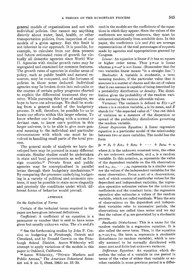
A THEORY OF THE BUDGETARY PROCESS 545

general models of organizations and not with individual policies. One cannot say anything directly about water, land, health, or other transportation policies, from inspection of our models of a given agency. But this limit is not inherent in our approach. It is possible, for example, to calculate from our data present and future estimated rates of growth for vir- tually all domestic agencies since World War II. Agencies with similar growth rates may be segregated and examined for common features. The growth rates of agencies in similar areas of policy, such as public health and natural re- sources, may be compared, and the fortunes of policies in those areas deduced. Individual agencies may be broken down into sub-units or the courses of certain policy programs charted to explain the differential treatment they re- ceive. While pursuing this type of analysis, we hope to have one advantage. We shall be work- ing from a general model of the budgetary process. It will, therefore, be possible for us to locate our efforts within this larger scheme. To know whether one is dealing with a normal or deviant case, to know one's position in this larger universe, is to be able to give more gen- eral meaning to the individual and particular circumstances with which one must be in- volved in handling small parts of the total pro- cess.

The general mode of analysis we have de- veloped here may be pursued in many different contexts. Similar studies could be undertaken in state and local governments as well as for- eign countries.27 Private firms and public agencies may be conceptualized in parallel terms through their budgetary mechanisms.28 By comparing the processes underlying budget- ing in a variety of political and economic sys- tems, it may be possible to state more elegantly and precisely the conditions under which dif- ferent forms of behavior would prevail.

APPENDIX

On the Definition of Terms

Certain of the technical terms required in the paper are here given informal definitions.

Coefficient: A coefficient of an equation is a parameter or number that is said to have some given but usually unknown value. The a's and $'s

27 See the forthcoming studies by John P. Cre- cine on budgeting in Pittsburgh, Detroit and Cleveland, and by Donald Gerwin on the Pitts- burgh School District. Aaron Wildavsky will attempt to apply variations of the models in this paper to Oakland, California.

28 Aaron Wildavsky, "Private Markets and Public Arenas," The American Behavioral Scien- tist vol. 9 no. 7. (SeDt. 1965) no. 33-39.

used in the models are the coefficients of the equa- tions in which they appear. Since the values of the coefficients are usually unknown, they must be estimated statistically from available data. In this paper, the coefficients (a's and f3's) are average representations of the real percentages of requests made by agencies and appropriations granted by Congress.

Linear: An equation is linear if it has no square or higher order terms. Thus y = ax is linear whereas = ax2 is not linear. (Remember that for two variables linear means "in a straight line.")

Stochastic: A variable is stochastic, a term meaning random, if the particular value that it assumes is a matter of chance and the set of values that it can assume is capable of being described by a probability distribution or density. The distri- bution gives the probability of the random vari- able assuming the various allowable values.

Variance: The variance is defined as E(x-M)2

where x is a random variable, ;i is its mean, and E stands for "the expected value of." One can think of variance as a measure of the dispersion or spread of the probability distribution governing the random variable. Linear Regression Equation: A linear regression equation is a particular model of the relationship between two or more variables. The model has the form

Yis = 0 + flxli + 62X2i + * + IkXki + Ei

where flo is the unknown constant term, the other

O's are unknown coefficients, and ej is a random variable. In this notation, yi represents the value of the dependent variable on the ith observation and xii, X2i, * * *, xki represents in a similar man- ner the values of the independent variables for the same observation. From a set of n observations, each of which consists of particular values for the dependent and independent variables, the regres- sion operation estimates values for the unknown coefficients and the constant term; the regression operation also estimates n values of the random variable, which are called residuals. When the sets of observations on the dependent and indepen- dent variables refer to successive periods, the observations are called time series and we say that the values of yi are generated by a stochastic process.

Stochastic Disturbance: This is a name for the random variable in a regression equation. It is also called the error term. Thus, in the equation y'= ax+et, the term et represents a stochastic disturbance (or random variable), which is usu- ally assumed to be normally distributed with mean zero and finite but unknown variance.

Difference Equation: An equation which de- scribes the value of a variable in one period in terms of the value of either that variable or an- other variable in some previous period is a differ-

546 THE AMERICAN POLITICAL SCIENCE REVIEW

ence equation. For example, xg = flyt-1 is a differ- ence equation. If a random variable is present, the equation is called a stochastic difference equation. Thus, if e is a random variable, x =iBytil+et is a stochastic difference equation and the successive values of x may be thought of as a stochastic process.

Unstable, Evolutionary or Explosive Process: A process is said to be unstable, evolutionary or explosive if the expected values of the successive values taken by the process are increasing. For example, the stochastic difference equation yt = yye-i +Et, where -y >1, generates an evolu- tionary process.

Serially Independent: If successive realizations of a random variable are serially independent, the value it assumes in one period is independent of the value it assumed in a previous period. This can be described mathematically as E(xt xt-1) =E(xt), meaning that the expected value of random variable x at period t does not depend upon the value that the random variable x as- sumed at period t -1. It follows that the expected simple correlation between xt and xti will be zero, if the random variable x is serially indepen- dent. For example, in our models, the assumption of serial independence of the disturbances reflects the belief that special circumstances in one year either do not affect special circumstances in suc- ceeding years or that their influence enters ex- plicitly into our model (as in equation (8) and the equations of footnote 4).

The Meaning of a Markov Process

For our purposes, a Markov process generating some random variable x, is a process for which the value of x at time t depends upon the values as- sumed by that random variable at one or more earlier periods plus the value assumed by some stochastic disturbance at time t. A Markov pro- cess is "first order" if the variable xt takes on a value that depends only upon the value of the variable xti- in the previous period plus the value of a stochastic disturbance at time t. Thus

Xi = aXt-1 + et

is a first order Markov process where et is a ran- dom variable with a given distribution and a is a non-zero constant. A second order Markov pro- cess can be described by

xt =ix t-1 + a2Xt-2 + 'Et

where both a, and a2 are non-zero constants. The value of the variable xt now depends upon its values in two previous periods.

On the Meaning of Goodness of Fit

An intuitive notion of good fit for a linear re- gression equation is that in a scatter diagram the

observations should cluster about the fitted line. Probably the most popular measure of good fit is the square of the multiple correlationcoefficient (R2), which may often be interpreted as the per- centage of the variance of the dependent variable that is explained by the postulated linear relation- ship (regression). For our models however, this interpretation is not valid, although the adjusted R gives a rough measure of the goodness of fit. The closer to 1 that the adjusted B is, the better the fit.

On Standard Deviations of Coefficient Estimates

Speaking roughly, these standard deviations measure the reliability of the estimates of the coefficients. The smaller the estimated standard deviation, the more accurate the estimated coeffi- cient is likely to be. If we had another series of data generated from the same process, the smaller the standard deviation of the coefficient (esti- mated from the first data) in relation to the size of this coefficient, the more likely it is that a new estimate made on the basis of the hypothetical new series of data would be close to the estimate made from the original data. Generally, one hopes the estimated standard deviation of the coefficient is at least as small as one-half the size of the esti- mated coefficient.

On Biased and Unbiased Estimators

Think of the problem of trying to determine the average IQ of students at a large university. Sup- pose the administration would not allow access to records and one did not wish to give IQ tests to all students. One might select a certain number of students at random (a sample) and give them the tests. The test scores of these students are sample observations. One might compute the average of these test scores and claim that he has an estimate of the mean IQ of all students at the University. The estimator is the formula for the average of the sample observations. If he repeated the process, taking a new sample, it is possible that the esti- mator would produce a slightly different estimate of the mean. However, the estimator would still have a certain expected value. If the expected value of the estimator can be proven to equal the population parameter (the mean IQ of all the students example) then the estimator is said to be unbiased. Otherwise, it is said to be biased.

On Consistent Estimators

An estimator is consistent if it approaches nearer and nearer to the true value of a parameter (in our case, a coefficient) as the size of the sample is increased. A consistent estimator may be biased (it may approach closer to but never actually equal the parameter), but if the sample from

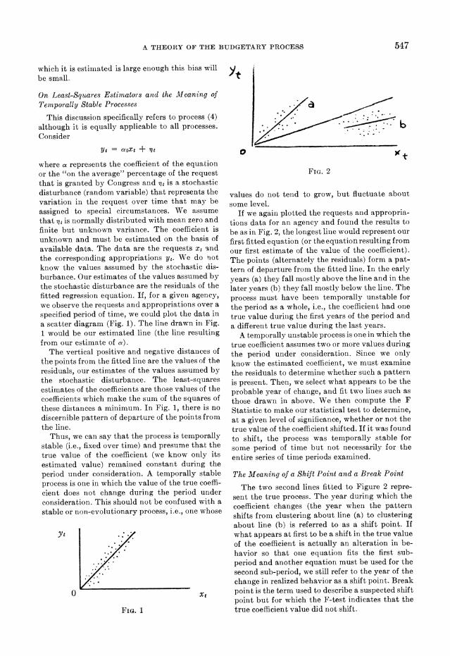
A THEORY OF THE BUDGETARY PROCESS 547

which it is estimated is large enough this bias will be small.

On Least-Squares Estimators and the Meaning of Temporally Stable Processes

This discussion specifically refers to process (4) although it is equally applicable to all processes. Consider

Yt aoxt + nt

where a represents the coefficient of the equation or the "on the average" percentage of the request that is granted by Congress and qt is a stochastic disturbance (random variable) that represents the variation in the request over time that may be assigned to special circumstances. We assume that 77t is normally distributed with mean zero and finite but unknown variance. The coefficient is unknown and must be estimated on the basis of available data. The data are the requests xt and the corresponding appropriations Yt. We do not know the values assumed by the stochastic dis- burbance. Our estimates of the values assumed by the stochastic disturbance are the residuals of the fitted regression equation. If, for a given agency, we observe the requests and appropriations over a specified period of time, we could plot the data in a scatter diagram (Fig. 1). The line drawn in Fig. 1 would be our estimated line (the line resulting from our estimate of a).

The vertical positive and negative distances of the points from the fitted line are the values of the residuals, our estimates of the values assumed by the stochastic disturbance. The least-squares estimates of the coefficients are those values of the coefficients which make the sum of the squares of these distances a minimum. In Fig. 1, there is no discernible pattern of departure of the points from the line.

Thus, we can say that the process is temporally stable (i.e., fixed over time) and presume that the true value of the coefficient (we know only its estimated value) remained constant during the period under consideration. A temporally stable process is one in which the value of the true coeffi- cient does not change during the period under consideration. This should not be confused with a stable or non-evolutionary process, i.e., one whose

;;t

0 Xt

FIG. 1

0b

FIG. 2

values do not tend to grow, but fluctuate about some level.

If we again plotted the requests and appropria- tions data for an agency and found the results to be as in Fig. 2, the longest line would represent our first fitted equation (or the equation resulting from our first estimate of the value of the coefficient). The points (alternately the residuals) form a pat- tern of departure from the fitted line. In the early years (a) they fall mostly above the line and in the later years (b) they fall mostly below the line. The process must have been temporally unstable for the period as a whole, i.e., the coefficient had one true value during the first years of the period and a different true value during the last years.

A temporally unstable process is one in which the true coefficient assumes two or more values during the period under consideration. Since we only know the estimated coefficient, we must examine the residuals to determine whether such a pattern is present. Then, we select what appears to be the probable year of change, and fit two lines such as those drawn in above. We then compute the F Statistic to make our statistical test to determine, at a given level of significance, whether or not the true value of the coefficient shifted. If it was found to shift, the process was temporally stable for some period of time but not necessarily for the entire series of time periods examined.

The Meaning of a Shift Point and a Break Point

The two second lines fitted to Figure 2 repre- sent the true process. The year during which the coefficient changes (the year when the pattern shifts from clustering about line (a) to clustering about line (b) is referred to as a shift point. If what appears at first to be a shift in the true value of the coefficient is actually an alteration in be- havior so that one equation fits the first sub- period and another equation must be used for the second sub-period, we still refer to the year of the change in realized behavior as a shift point. Break point is the term used to describe a suspected shift point but for which the F-test indicates that the true coefficient value did not shift.